Analytical fits for the synchrotron emission from a power-law particle distribution with a sharp cutoff

Fouka, M.; Ouichaoui, S.

doi:10.1093/mnras/stu922

Abstract

In several high-energy astrophysical sites, shocks are assumed to produce a power-law distribution of accelerated charged particles (e.g., electrons, protons) and to generate mild to strong magnetic fields, which favours synchrotron emission. For such environments and conditions, we have performed and present here four practical formulas, with different levels of accuracy, for fitting the synchrotron spectral power radiated by a pure power-law particle distribution, with isotropic pitch angle distribution. The first three ones can be useful compared to the fourth one, because of their simplicity, in the case of particle distribution with no high-energy cutoff. However, the fourth formula, the more accurate one, can be of great interest for astrophysical applications (even though it is more complicated) for the more general case of a power-law distribution with high-energy sharp cutoff. The latter is derived for index p within the range, 1 < p < 6, with maximum relative error of less than 0.5 per cent in the case of infinite energy range and of less than 8.2 per cent in the more general case of particle energy with sharp cutoff. The latter is expressed in terms of parameters as functions of index p. These parameters have been fitted with adopting the Levenberg–Marquardt algorithm in log–log scale. According to these formulas, initially derived for the total spectral power, we have then derived (1) the degree of polarization, (2) cooling spectra for a broken power-law distribution and (3) synchrotron self-absorption spectra for both the broken and non-broken power-law distributions. The proposed expressions are relevant for non-thermal astrophysical sources in the sense that by using them one avoids usually complicated and long CPU time calculations, without performing any integration.

radiation mechanisms: non-thermal, methods: analytical

1 INTRODUCTION

Relativistic shocks such as those at work behind gamma-ray bursts (GRB), pulsar wind nebulae or active galactic nuclei and even non-relativistic ones as in supernova remnants (SNRs), are thought to be potential sources of particle acceleration in the universe (Gallant & Achterberg 1999; Spitkovsky 2008). Charged particles accelerated via these shocks are often described by a power-law distribution, with isotropic pitch angle distribution, of the type N(γ) = Cγ^−p, in function of the Lorentz factor with sharp cutoff, i.e. γ₁ < γ < γ₂ (Fermi 1949; Blanford & Ostriker 1978; Gallant 2002; Petrosian & Bykov 2008), where the values of index p are however not well known although numerical simulations have led to typical values p ∼ 2.2-2.3 for relativistic shocks (see e.g. Gallant et al. 2000; Guthmann et al. 2000) and p = 2 for non-relativistic ones (Fermi 1949). This is possible in highly turbulent shocks usually dominated by intense magnetic fields (Ostrowski & Bednarz 2002). However, careful numerical simulations (Sironi, Spitkovsky & Arons 2013) have led to a particle distribution downstream the shock well described by a Maxwellian plus a non-thermal tail with slope of ∼2.4 ± 0.1 whose high-energy part can be adjusted by an exponential cutoff leading to the general form, N(γ) = Cγ^{− p}exp( − γ/γ_c), with γ > γ₁. Nevertheless, for our purpose in this paper, we have considered only a power-law distribution with sharp cutoff because of the simplicity of the corresponding analytical treatment, whereas the case of a power-law distribution with exponential cutoff that involves an additional parameter (γ_c) may be the subject of a future contribution. Then, we have considered index p values within the wide range, 1 < p < 6, surely containing values of astrophysical interest. The computation of the synchrotron spectral power from a power-law particle distribution (mainly electrons and protons) in astrophysical sites dominated by relativistic shocks can be made by numerical integration of the synchrotron function, F(x) (see equation 2), through the particle power-law distribution. To avoid performing complicated integrals (and then gain CPU time), we here propose an accurate analytical fit based on the asymptotic forms of the integrated spectral power for low- and high frequency values. In Section 2, we present the most adequate dimensionless form of the integrated spectral power together with corresponding asymptotic forms. Then, we report, in Section 3, the fit procedure used and the derived results. In Section 4, we present additional analytical fit related to the complementary synchrotron function, G(x), in order to treat the polarization. The derived result for the synchrotron self-absorption (SSA) is presented in Section 5. Then, we treat the case of a broken power law which is indispensable for cooling spectra in Section 6 before concluding in Section 7.

2 SYNCHROTRON POWER FROM A POWER-LAW PARTICLE DISTRIBUTION

The instantaneous (adiabatic) integrated synchrotron spectral power radiated by a pure power-law particle distribution with isotropic pitch angle distribution is written as (Rybicki & Lightman 1979)

\begin{equation} P_{\nu }=\frac{2\pi \sqrt{3}e^{2}\nu _{{\rm L}}}{c}\int _{\gamma _{1}}^{\gamma _{2}}{\rm d}\gamma C\gamma ^{-p}F\left( \frac{\nu }{\nu _{{\rm c}}}\right), \end{equation}

(1)

where ν_L = eB/2πmc and ν_c ≡ ν_c(γ) = (3/2)γ²ν_L are, respectively, the Larmor gyration frequency and the synchrotron characteristic frequency for a radiating charged particle with Lorentz factor γ, the usual quantities (m, e, c and B) denoting, respectively, the particle rest mass, its electric charge, the velocity of light in vacuum and the averaged strength of the perpendicular component of the magnetic field relative to the particle velocity direction. The synchrotron function, F(x), is given by (Westfold 1959; Jackson 1962; Rybicki & Lightman 1979)

\begin{equation} \displaystyle {} F(x)=x\int _{x}^{\infty }K_{5/3}(x^{\prime }){\rm d}x^{\prime }, \end{equation}

(2)

in terms of the dimensionless frequency, x ≡ x(γ) = ν/ν_c(γ), and the modified, non-integer order Bessel function, K_5/3(x) (see e.g. Abramowitz & Stegun 1965). One notes that the synchrotron function expressed by equation (2) is a pure classical result, valid for relativistic energies (γ ≫ 1) and magnetic field strengths below the quantum critical limit, |$B_{ {\rm cr}}=m_{{\rm e}}^{2}c^{3}/e\hbar =4.41\times 10^{13}$| G, i.e. B ≪ B_cr. In contrast, in the case of low energies, the synchrotron version is replaced by the cyclotron emission, and in the case of very strong magnetic field, B ≳ B_cr, quantum electrodynamic effects must be incorporated (see e.g. Brainerd 1987; Brainerd & Petrosian 1987).

We first focus on the instantaneous (adiabatic) spectrum if all radiating particles are adiabatic and, then, cooling effects can be ignored. Indeed, instantaneous spectra are valid when the observation time-scale is much more lower than the synchrotron emission one, which can be the case, e.g., of SNRs and late afterglows following the GRB prompt emission. Then, cooling spectra can be easily deduced by just considering a broken power-law particle distribution, a case treated here in Section 6.

As we have shown previously (Fouka & Ouichaoui 2009, 2011), in formula (1), P_ν can be expressed as

\begin{equation} P_{\nu }=P_{1} F_{p}(x,\eta ), \end{equation}

(3)

in terms of the parametric function F_p(x, η) with here x = ν/ν₁ (where |$\nu _{1}=(3/2)\gamma _{1}^{2}\nu _{{\rm L}}$|⁠) and η = γ₂/γ₁, whereas the normalization coefficient, P₁, is given by

\begin{equation} P_{1} = \pi \sqrt{3}e^{2}\nu _{{\rm L}}\gamma _{1}^{-p+1}\frac{C}{c}. \end{equation}

(4)

Besides, function F_p(x, η) can be split as (Fouka & Ouichaoui 2009)

\begin{equation} F_{p}(x,\eta )=F_{p}(x)-\eta ^{-p+1}F_{p}(x/\eta ^{2}) \end{equation}

(5)

for pointing out function F_p(x), which is of central interest in this work. This function can be expressed as (Fouka & Ouichaoui 2009)

\begin{equation} F_{p}(x)=x^{-(p-1)/2}\int _{0}^{x}x^{\prime (p-3)/2}F(x^{\prime })\,\rm{d}x^{\prime }. \end{equation}

(6)

It has the following asymptotic forms (Fouka & Ouichaoui 2009)

\begin{equation} F_{p}(x) \approx \left\lbrace \begin{array}{lll} A_{1}(x) = & \kappa _{p}x^{1/3} &\quad {\rm for}\ x\ll 1\\ A_{2}(x) = & C_{p}x^{-(p-1)/2} &\quad {\rm for}\ x\gg 1 \end{array} \right., \end{equation}

(7)

where (Rybicki & Lightman 1979; Fouka & Ouichaoui 2009)

\begin{equation} \left\lbrace \begin{array}{l} \displaystyle \kappa _{p}=\frac{2F_{1}}{p-1/3} \\ \displaystyle C_{p}=\frac{2^{(p+1)/2}}{p+1}\:\Gamma \left( \frac{p}{4}+\frac{19}{12}\right)\Gamma \left(\frac{p}{4}-\frac{1}{12}\right) \end{array} \right., \end{equation}

(8)

in terms of the Gamma function and coefficient |$F_{1}=\pi 2^{5/3}/\sqrt{3}\Gamma (1/3)$|⁠.

3 ANALYTICAL FITS

In this section, we present and discuss four different possible analytical fits for functions F_p(x) and F_p(x, η) with different levels of accuracy.

3.1 The first form

This form is based on the simplest approximation of the synchrotron function, F(x), that can be written as

\begin{equation} F(x) \approx \left\lbrace \begin{array}{ll} F_{1}x^{1/3} &\quad {\rm for}\ x\le x_{0} \\ 0 &\quad {\rm for}\ x> x_{0} \end{array} \right., \end{equation}

(9)

where x₀ is a specific value defined such that the area under the approximate form, noted A_F, is the same as that of the exact total area under function F(x). One obtains A_F = (4/9)Γ(1/3)Γ(2/3), leading to x₀ = (4A_F/3F₁)^3/4 ≈ 1.

Then, upon integration (see equation 6), one obtains the following approximate form for function F_p(x)

\begin{equation} F_{p}(x) \approx \left\lbrace \begin{array}{ll} \kappa _{p}x^{1/3} &\quad {\rm for}\ x\le 1\\ \kappa _{p}x^{-(p-1)/2} &\quad {\rm for}\ x > 1 \end{array} \right.. \end{equation}

(10)

According to this expression and to equation (7), the relative error (defined by, error = |F_approx − F_exact|/F_exact) for large x-values (x ≫ 1) is ∼1 − (κ_p/C_p) which, e.g. for p = 2.5, yields 13.8 per cent, whereas the maximum error, ≈85 per cent, is very large. Fig. 1 depicts the relative errors for this form (solid line) together with those associated with the three other following forms (presented in Sections 3.2–3.4) for index p = 2.5.

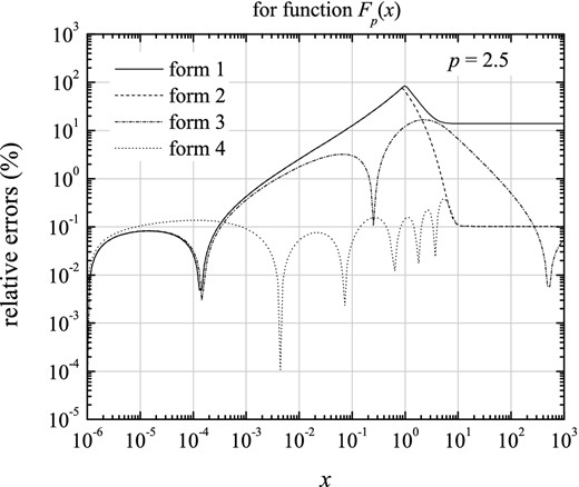
Figure 1.

The four relative errors associated with the proposed four fitting forms of F_p(x) for index p = 2.5: solid line for the first form (equation 10), dashed line for the second form (equation 12), dash–dotted line for the third form (equation 14) and dotted line for the fourth (more accurate) form (equation 16).

Open in new tab Download slide

Then, according to equation (5), the corresponding approximate form for function F_p(x, η) in the case of finite η is written as

\begin{equation} F_{p}(x,\eta ) \approx \left\lbrace \begin{array}{ll} \kappa _{p}\left(1-\eta ^{-p+\frac{1}{3}} \right) x^{1/3} &\quad {\rm for}\ x\le 1 \\ \kappa _{p}x^{-(p-1)/2} - \kappa _{p} \eta ^{-p+\frac{1}{3}} x^{1/3} &\quad {\rm for}\ 1 <x < \eta ^{2} \\ 0 &\quad {\rm for} \ x > \eta ^{2} \end{array} \right.. \end{equation}

(11)

The latter results in a sharp cutoff in the total spectrum above the frequency x = η², and then to a relative error of 100 per cent, compared to the exact result. The corresponding relative error to this form is depicted in Fig. 6 (solid line), together with the three other following forms (presented in Sections 3.2–3.4) for index p = 2.5 and η = 100. Consequently, in the case of particle distribution with sharp cutoff, this form can be used just for rapid estimation of spectra, but not for moderate or accurate calculations.

3.2 The second form

For this form, function F_p(x) is approximated by the first asymptotic form, A₁(x), up to a value x_in and by the second asymptotic form, A₂(x), behind x_in, i.e.

\begin{equation} F_{p}(x) \approx \left\lbrace \begin{array}{ll} \kappa _{p}x^{1/3} &\quad {\rm for}\ x\le x_{ {\rm in}}\\ C_{p}x^{-(p-1)/2} &\quad {\rm for}\ x > x_{ {\rm in}} \end{array} \right., \end{equation}

(12)

where x_in = (C_p/κ_p)^{2/(p − 1/3)} is defined as the intersection abscissa of the two asymptotic forms. Values of index p ∼ 3 give κ_p ∼ C_p and, then, x_in ∼ 1 for which this approximate expression (equation 12) becomes the same as the first one (equation 10). For this form, the maximum relative error for index p = 2.5 is ≈77 per cent, which is slightly lower than that of the first form. However, as shown in Fig. 1, for index p = 2.5, this form (dashed line) is better than the first form (solid line) for fitting the high-frequency range (x ≫ 1), with lower relative error, ∼0.1 per cent, compared to that of the first form, ∼13.8 per cent.

Then, according to equation (5), the corresponding approximate form for function F_p(x, η) in the case of finite η is written as

\begin{equation} F_{p}(x,\eta ) \approx \left\lbrace \begin{array}{ll} \kappa _{p}\left(1-\eta ^{-p+\frac{1}{3}} \right) x^{1/3} &\quad {\rm for}\ x\le x_{ {\rm in}} \\ C_{p}x^{-(p-1)/2} - \kappa _{p} \eta ^{-p+\frac{1}{3}} x^{1/3} &\quad {\rm for}\ x_{ {\rm in}} <x < \eta ^{2} x_{ {\rm in}} \\ 0 &\quad {\rm for}\ x > \eta ^{2} x_{ {\rm in}} \end{array} \right.. \end{equation}

(13)

The latter is very similar to that of the first form. It results in a sharp cutoff above the frequency x = η²x_in, leading to an error of 100 per cent for the range x > η²x_in. It is therefore not recommended for moderate or accurate calculations, in the case of particle distribution with sharp cutoff.

3.3 The third form

This form is simply derived from the asymptotic forms of function F_p(x) and is given by

\begin{equation} \begin{array}{ll} F_{p}(x) & \approx \left[ A_{1}^{-1}(x) + A_{2}^{-1}(x) \right] ^{-1} = \frac{ \kappa _{p}x^{1/3} }{1+ \displaystyle {\frac{\kappa _{p}}{C_{p}}} x^{(p-\frac{1}{3})/2} }. \end{array} \end{equation}

(14)

The maximum relative error corresponding to this form is ∼16 per cent. This form is better and more accurate compared to the two preceding ones, as can be clearly seen in Fig. 1 (dash–dotted line) for η = ∞.

Then, according to equation (5), the corresponding approximate form for function F_p(x, η) in the case of finite η is written as

\begin{equation} F_{p}(x,\eta ) \approx \displaystyle {} \frac{ \kappa _{p}\left(\eta ^{p-\frac{1}{3}}-1\right) x^{1/3} }{\left[ 1+ \displaystyle {\frac{\kappa _{p}}{C_{p}}} x^{(p-\frac{1}{3})/2} \right] \left[ \eta ^{p-\frac{1}{3} }+ \displaystyle {\frac{\kappa _{p}}{C_{p}}} x^{(p-\frac{1}{3})/2} \right] }. \end{equation}

(15)

The latter form, corresponding to the general case of a particle distribution with sharp cutoff, is not sufficiently accurate, more especially for the high-frequency range, x > η², for which the relative error increases significantly, as reported by Fig. 6.

This constitutes the main reason pushing us to look for more accurate fit formula with high/moderate accuracy (with a maximum relative error not exceeding few per cent) for all frequency ranges, and for any couple of (p, η) parameters with η ≳ 3 and index p in the range 1 < p < 6.

3.4 The fourth form

For this form, which is the most accurate compared to the preceding ones (even though it is more complicated), the central idea in fitting function F_p(x) is to express the latter in terms of its asymptotic forms as

\begin{equation} F_{p}(x) \approx A_{1}(x)\delta _{1}(x)+A_{2}(x)\delta _{2}(x) , \end{equation}

(16)

where δ₁(x) and δ₂(x) are two arbitrary functions, which must verify the following respective limits, i.e.

\begin{equation} \delta _{1}(x)\approx \left\lbrace \begin{array}{l}1\ \ \ {\rm for}\ \ \ x\ll 1 \\ 0\ \ \ {\rm for}\ \ \ x\gg 1 \end{array} \right. \end{equation}

(17)

and

\begin{equation} \delta _{2}(x)\approx \left\lbrace \begin{array}{l}0\ \ \ {\rm for}\ \ \ x\ll 1 \\ 1\ \ \ {\rm for}\ \ \ x\gg 1 \end{array} \right.. \end{equation}

(18)

As adequate forms of functions δ₁ and δ₂, we propose, respectively, the following expressions

\begin{equation} \delta _{1}(x)= \exp \left( \sum _{k=1}^{n_{1}}a_{k}x^{2/k} \right) \end{equation}

(19)

and

\begin{equation} \delta _{2}(x)= \left[ 1-\exp \left( \sum _{k=1}^{n_{2}}b_{k}x^{2/k} \right) \right]^{p/5+1/2}. \end{equation}

(20)

Note that the same analytical fit procedure has been adopted by Fouka & Ouichaoui (2013) to account for the synchrotron function, F(x), and its complementary function, G(x) = xK_2/3(x). The index {p/5 + 1/2} appearing in the expression of δ₂(x) (see equation 20) has been found after numerical investigations aiming at obtaining the lowest possible values of the relative error for the whole range of index p considered (i.e. 1 < p < 6). In order to extract coefficients a_k and b_k for a given couple of orders (n₁, n₂), we proceeded by chi-squares minimization with adopting the Levenberg–Marquardt algorithm (Levenberg 1944; Marquardt 1963) in log–log scale and, then, considered coefficients a_k and b_k as functions of index p, which has led us to an adequate and satisfactory result with n₁ = 3 and n₂ = 1. Each coefficient could be adjusted by a polynomial fit of order 3 or 4 to ensure a good accuracy in the general case when η is finite, according to equation (5). These coefficients are given by

\begin{equation} \begin{array}{llllll} & &\quad \times p &\quad \times p^{2} &\quad \times p^{3} &\quad \times p^{4} \\ a_{1}= &\quad -0.146\,02 &\quad +3.623\,07\times 10^{-2} &\quad -5.765\,07\times 10^{-3} &\quad +3.469\,26\times 10^{-4} &\quad \\ a_{2}= &\quad -0.366\,48 &\quad +0.180\,31 &\quad -7.307\,73\times 10^{-2} &\quad +1.124\,84\times 10^{-2} &\quad -6.176\,83\times 10^{-4} \\ a_{3}= &\quad +9.693\,76\times 10^{-2} &\quad -0.488\,92 &\quad +0.140\,24 &\quad -1.936\,78\times 10^{-2} &\quad +1.015\,82\times 10^{-3} \\ b_{1}= &\quad -0.202\,50 &\quad +5.434\,62\times 10^{-2} &\quad -8.441\,71\times 10^{-3} &\quad +5.212\,81\times 10^{-4} &\quad \\ \end{array} \end{equation}

(21)

as polynomial fits, and plotted in Fig. 2 versus index p. Then, the final fitting formula for function F_p(x) is written as

\begin{equation} \begin{array}{ll} F_{p}(x)\approx & \kappa _{p}x^{1/3}\exp ({a_{1}x^{2}+a_{2}x+a_{3}x^{2/3}}) +C_{p}x^{-(p-1)/2} [1-\exp (b_{1}x^{2}) ]^{p/5+1/2} \end{array}. \end{equation}

(22)

Coefficients a1, a2, a3 and b1 as functions of index p, for function Fp(x), with corresponding polynomial fits reported by equation (21).

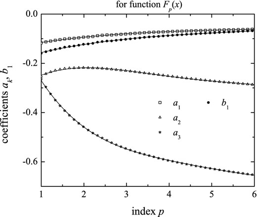
Figure 2.

Coefficients a₁, a₂, a₃ and b₁ as functions of index p, for function F_p(x), with corresponding polynomial fits reported by equation (21).

Open in new tab Download slide

The maximum relative error resulting in fitting expression (22) to function F_p(x) is reported in Fig. 3 versus index p. The latter does not exceed 0.5 per cent, for the whole considered range of index p.

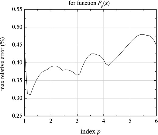
Figure 3.

The maximum relative error in fitting function F_p(x) versus index p, according to the fourth form (equation 22). This error does not exceed 0.5 per cent for the whole range of index p, 1 < p < 6.

Open in new tab Download slide

As stated, one is concerned about calculating the radiated spectral power for a particle distribution with sharp cutoff, i.e. finite γ₂. Indeed, function F_p(x) corresponds to the simplest case of infinite Lorentz factor, γ₂ = ∞. Thus, in the general case, i.e. γ₂ ≠ ∞, one has just to use equation (5) for calculating the spectral power.

However, in the general case (η ≠ ∞), function F_p(x, η) calculated from equations (5) and (22) takes on negative values for high frequencies, x ≫ η². In order to solve this problem, we have used the asymptotic form of function F_p(x, η) for the frequency range x ≫ η², given by (Fouka & Ouichaoui 2009, 2011)

\begin{equation} F_{p}(x,\eta )\approx \sqrt{\frac{\pi }{2}}\eta ^{-p+2}x^{-1/2}{\rm e}^{-x/\eta ^{2}}\left[1+ \frac{55}{72}\left(\frac{x}{\eta ^{2}}\right)^{-1}\right], \end{equation}

(23)

where coefficient 55/72 is to be replaced by a coefficient a_p in order to improve the accuracy of the final approximate formula.

Finally, the more general fit formula for function F_p(x, η) is given by

\begin{equation} F_{p}(x,\eta )\approx \left\lbrace \begin{array}{ll} F_{p}(x)-\eta ^{-p+1}F_{p}(x/\eta ^{2}) &\quad {\rm for}\ x < x_{{\rm c}} \\ \displaystyle {}\sqrt{\frac{\pi }{2}}\eta ^{-p+2}x^{-1/2}{\rm e}^{-x/\eta ^{2}}\left[1+ a_{p}\left(\frac{x}{\eta ^{2}}\right)^{-1}\right]&\quad {\rm for}\ x \ge x_{{\rm c}} \end{array} \right., \end{equation}

(24)

where function F_p(x) can be calculated according to equation (22) and the critical x_c-value corresponds to the approximate numerical solution of the equality

\begin{equation} F_{p}(x)-\eta ^{-p+1}F_{p}(x/\eta ^{2})=\sqrt{\frac{\pi }{2}} \eta ^{-p+2} x^{-1/2} {\rm e}^{-x/\eta ^{2}}, \end{equation}

(25)

given with coefficient a_p, versus index p, by

\begin{equation} \left\lbrace \begin{array}{l} x_{{\rm c}}= (2.028 -1.187\ p +0.240\ p^{2})\eta ^{2} \\ a_{p}= -0.033-0.104\ p+0.115\ p^{2} \end{array} \right.. \end{equation}

(26)

As an example, we report in Fig. 4 function F_p(x, η) (circles) for index p = 2.5 and η = 100 together with the corresponding fit (solid line) according to equation (24). According to equation (24), the maximum relative error for function F_p(x, η) in the more general case (with η ≳ 3) is 8.2 per cent, as is reported by Fig. 5. For a given couple (p, η), the maximum error is around x_c, as is reported in Fig. 6, for index p = 2.5 and η = 100.

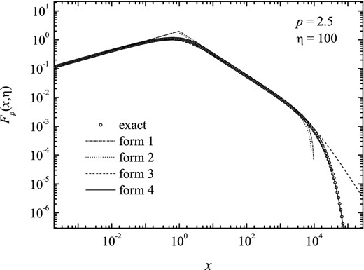
Figure 4.

Function F_p(x, η) for index p = 2.5 and η = 100, calculated numerically and adjusted according to the four forms.

Open in new tab Download slide

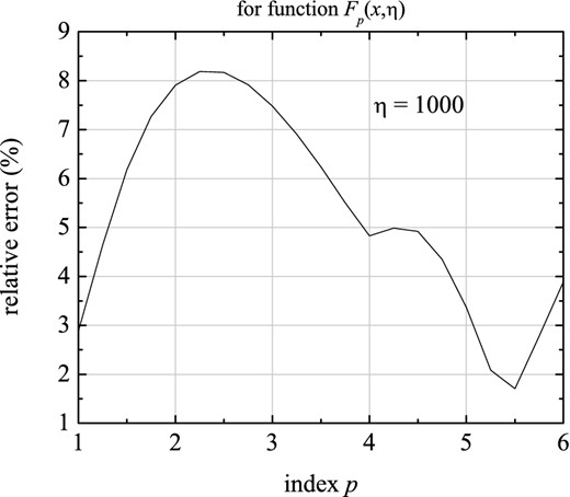
Figure 5.

The maximum relative error in fitting function F_p(x, η), versus index p, for η = 100, according to the fourth form (equations 22 and 24). It does not exceed 8.2 per cent, for 1 < p < 6 and η ≳ 3.

Open in new tab Download slide

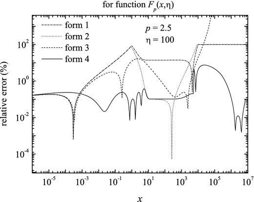
Figure 6.

The relative errors in fitting function F_p(x, η), for index p = 2.5 and η = 100, between the numerical computation of F_p(x, η) and the four approximate forms. This clearly reveals that the fourth form (equations 22 and 24) is the most accurate one for the whole frequency ranges (even though it is more complicated, compared to the other forms), and can then be used for astrophysical applications without any care. For p = 2.5, η = 100, the maximum error for the fourth form is <8.2 per cent.

Open in new tab Download slide

$Coefficients $a^{\prime }_{1}$, $a^{\prime }_{2}$, $a^{\prime }_{3}$ and $b^{\prime }_{1}$ as functions of index p for function Gp(x) with corresponding polynomial fits reported by equation (41).$

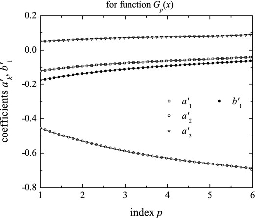
Figure 7.

Coefficients |$a^{\prime }_{1}$|⁠, |$a^{\prime }_{2}$|⁠, |$a^{\prime }_{3}$| and |$b^{\prime }_{1}$| as functions of index p for function G_p(x) with corresponding polynomial fits reported by equation (41).

Open in new tab Download slide

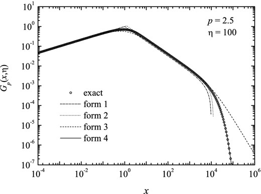
Figure 8.

Function G_p(x, η) for index p = 2.5 and η = 100, calculated numerically and adjusted according to the four forms.

Open in new tab Download slide

4 DEGREE OF POLARIZATION

The degree of polarization is often an indispensable physical quantity that needs to be determined (computed and/or measured) in order to distinguish between radiation processes characterized by similar spectral shapes. It is defined by

\begin{equation} \Pi _{\nu } =\frac{ P_{ \nu }^{\bot }-P_{ \nu }^{\Vert } }{ P_{ \nu }^{\bot }+P_{ \nu }^{\Vert }}, \end{equation}

(27)

where |$P_{ \nu }^{\bot }$| and |$P_{ \nu }^{\Vert }$| are, respectively, the radiated powers in the perpendicular and parallel directions relative to that of the magnetic field. For a power-law particle distribution with index p and finite energy range (i.e. finite η), one has

\begin{equation} \left\lbrace \begin{array}{l}P_{ \nu }^{\bot }+P_{ \nu }^{\Vert } \propto F_{p}(x,\eta ) \\ P_{ \nu }^{\bot }-P_{ \nu }^{\Vert } \propto G_{p}(x,\eta ) \end{array} \right., \end{equation}

(28)

where function G_p(x, η) is defined in similar way as function F_p(x, η) and can be written as

\begin{equation} G_{p}(x,\eta )=G_{p}(x)-\eta ^{-p+1}G_{p}(x/\eta ^{2}), \end{equation}

(29)

in terms of function G_p(x) given by

\begin{equation} G_{p}(x)=x^{-(p-1)/2}\int _{0}^{x}x^{\prime (p-3)/2}G(x^{\prime }){\rm d}x^{\prime }, \end{equation}

(30)

where G(x) = xK_2/3(x) is the complementary synchrotron function (Westfold 1959) expressed in terms of the modified Bessel function K_2/3(x). Function G_p(x) admits the following asymptotic forms (Rybicki & Lightman 1979)

\begin{equation} G_{p}(x) \approx \left\lbrace \begin{array}{lll} A^{\prime }_{1}(x)= & \kappa ^{\prime }_{p}x^{1/3} &\quad {\rm for}\ x\ll 1\\ A^{\prime }_{2}(x)= & C^{\prime }_{p}x^{-(p-1)/2} &\quad {\rm for}\ x\gg 1 \end{array} \right. \end{equation}

(31)

with

\begin{equation} \left\lbrace \begin{array}{l}\displaystyle \kappa ^{\prime }_{p}=\frac{2G_{1}}{p-1/3} \\ \displaystyle C^{\prime }_{p}=2^{(p-3)/2} \Gamma \left( \frac{p}{4}+\frac{7}{12}\right)\Gamma \left(\frac{p}{4}-\frac{1}{12}\right) \end{array} \right., \end{equation}

(32)

where G₁ = F₁/2.

Then, in its general form the degree of polarization is written simply as

\begin{equation} \Pi (x,\eta ) =\frac{ F_{p}(x,\eta ) }{ G_{p}(x,\eta ) }. \end{equation}

(33)

4.1 Approximate formulas for function G_p(x, η)

We first, present approximate formulas for function G_p(x), and then deduce those for function G_p(x, η). Indeed, function G_p(x) can be fitted using the same method adopted for function F_p(x), and can then be approximated by the forms described below.

4.1.1 The first form

This form is similar to that for function F_p(x) expressed by equation (10), and is given by

\begin{equation} G_{p}(x) \approx \left\lbrace \begin{array}{ll} \kappa ^{\prime }_{p}x^{1/3} &\quad {\rm for}\ x\le 1\\ \kappa ^{\prime }_{p}x^{-(p-1)/2} &\quad {\rm for}\ x > 1 \end{array} \right., \end{equation}

(34)

whereas, for finite values of parameter η, it is written as

\begin{equation} G_{p}(x,\eta ) \approx \left\lbrace \begin{array}{ll} \kappa ^{\prime }_{p}\left(1-\eta ^{-p+\frac{1}{3}} \right) x^{1/3} &\quad {\rm for}\ x\le 1 \\ \kappa ^{\prime }_{p}x^{-(p-1)/2} - \kappa ^{\prime }_{p} \eta ^{-p+\frac{1}{3}} x^{1/3} &\quad {\rm for}\ 1 <x < \eta ^{2} \\ 0 &\quad {\rm for} \ x > \eta ^{2} \end{array} \right.. \end{equation}

(35)

4.1.2 The second form

This form is similar to that for function F_p(x) expressed by equation (12), and is given by

\begin{equation} G_{p}(x) \approx \left\lbrace \begin{array}{ll} \kappa ^{\prime }_{p}x^{1/3} &\quad {\rm for}\ x\le x^{\prime }_{ {\rm in}}\\ C^{\prime }_{p}x^{-(p-1)/2} &\quad {\rm for}\ x > x^{\prime }_{ {\rm in}} \end{array} \right., \end{equation}

(36)

where |$x^{\prime }_{ {\rm in}}=(C^{\prime }_{p}/\kappa ^{\prime }_{p})^{2/(p-1/3)}$| is defined as the intersection abscissa of the two asymptotic forms.

Then, according to equation (29), the corresponding approximate form to function G_p(x, η) in the case of sharp cutoff is written as

\begin{equation} G_{p}(x,\eta ) \approx \left\lbrace \begin{array}{ll} \kappa ^{\prime }_{p}\left(1-\eta ^{-p+\frac{1}{3}} \right) x^{1/3} &\quad {\rm for}\ x\le x^{\prime }_{ {\rm in}} \\ C^{\prime }_{p}x^{-(p-1)/2} - \kappa ^{\prime }_{p} \eta ^{-p+\frac{1}{3}} x^{1/3} &\quad {\rm for}\ x^{\prime }_{ {\rm in}} <x < \eta ^{2} x^{\prime }_{ {\rm in}} \\ 0 &\quad {\rm for}\ x > \eta ^{2} x^{\prime }_{ {\rm in}} \end{array} \right.. \end{equation}

(37)

4.1.3 The third form

This form is similar to that for function F_p(x) expressed by equation (14), and is given by

\begin{equation} G_{p}(x) \approx \displaystyle {} \frac{ \kappa ^{\prime }_{p}x^{1/3} }{1+ \displaystyle {\frac{\kappa ^{\prime }_{p}}{C^{\prime }_{p}}} x^{(p-\frac{1}{3})/2} }. \end{equation}

(38)

Then, according to equation (29), the corresponding approximate form for function G_p(x, η) in the case of finite η is written as

\begin{equation} G_{p}(x,\eta ) \approx \displaystyle {} \frac{ \kappa ^{\prime }_{p}\left(\eta ^{p-\frac{1}{3}}-1\right) x^{1/3} }{\left[ 1+ \displaystyle {\frac{\kappa ^{\prime }_{p}}{C^{\prime }_{p}}} x^{(p-\frac{1}{3})/2} \right] \left[ \eta ^{p-\frac{1}{3} }+ \displaystyle {\frac{\kappa ^{\prime }_{p}}{C^{\prime }_{p}}} x^{(p-\frac{1}{3})/2} \right] }. \end{equation}

(39)

4.1.4 The fourth form

This form is similar to that for function F_p(x) expressed by equation (22), and is given by

\begin{equation} \begin{array}{ll} G_{p}(x)\approx & \kappa ^{\prime }_{p}x^{1/3}\exp \left({a^{\prime }_{1}x^{2}+a^{\prime }_{2}x+a^{\prime }_{3}x^{2/3}}\right) + C^{\prime }_{p}x^{-(p-1)/2} \left[1-\exp \left(b^{\prime }_{1}x^{2} \right) \right]^{p/5+1/2} \end{array}, \end{equation}

(40)

for which the resulting fit coefficients, |$a^{\prime }_{1}$|⁠, |$a^{\prime }_{2}$|⁠, |$a^{\prime }_{3}$| and |$b^{\prime }_{1}$|⁠, are given by

\begin{equation} \begin{array}{llllll} & &\quad \times p &\quad \times p^{2} &\quad \times p^{3} &\quad \times p^{4} \\ a^{\prime }_{1}= &\quad -0.161\,03 &\quad +4.749\,25\times 10^{-2} &\quad -8.187\,73\times 10^{-3} &\quad +6.002\,02\times 10^{-4} &\quad \\ a^{\prime }_{2}= &\quad -0.356\,24 &\quad -0.108\,71 &\quad +1.070\,49\times 10^{-2} &\quad +1.780\,08\times 10^{-4} &\quad -8.196\,32\times 10^{-5} \\ a^{\prime }_{3}= &\quad +4.389\,23\times 10^{-2} &\quad +2.208\,71\times 10^{-4} &\quad +8.734\,37\times 10^{-3} &\quad -2.578\,72\times 10^{-3} &\quad +2.219\,10\times 10^{-4} \\ b^{\prime }_{1}= &\quad -0.224\,74 &\quad +5.947\,23\times 10^{-2} &\quad -8.920\,85\times 10^{-3} &\quad +5.845\,34\times 10^{-4} &\quad \\ \end{array} \end{equation}

(41)

as polynomial functions of index p with 1 < p < 6, and plotted by Fig. 7, whereas Fig. 8 depicts function G_p(x, η) calculated numerically and adjusted according to equation (42), for index p = 2.5 and η = 100. The maximum relative error resulting in fitting expression (40) to function G_p(x) is reported in Fig. 9 versus index p. The latter does not exceed 0.6 per cent, for the whole considered range of index p.

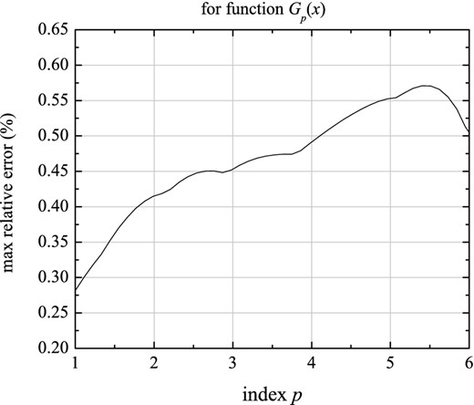
Figure 9.

The maximum relative error in fitting function G_p(x) versus index p, according to equation (40). This error does not exceed 0.6 per cent for the considered whole range of index p, 1 < p < 6.

Open in new tab Download slide

Finally, similarly as we have shown for function F_p(x, η) (see equation 24), the more general fitting formula for function G_p(x, η) is given by

\begin{equation} G_{p}(x,\eta )\approx \left\lbrace \begin{array}{ll} G_{p}(x)-\eta ^{-p+1}G_{p}(x/\eta ^{2}) &\quad {\rm for}\ x < x^{\prime }_{{\rm c}} \\ \displaystyle {}\sqrt{\frac{\pi }{2}}\eta ^{-p+2}x^{-1/2}{\rm e}^{-x/\eta ^{2}}\left[1+ a^{\prime }_{p}\left(\frac{x}{\eta ^{2}}\right)^{-1}\right]&\quad {\rm for}\ x \ge x^{\prime }_{{\rm c}} \end{array} \right., \end{equation}

(42)

where function G_p(x) can be calculated, as was the case for function F_p(x), by equation (40), with |$x^{\prime }_{{\rm c}}$| and |$a^{\prime }_{p}$| given by

\begin{equation} \left\lbrace \begin{array}{l} x^{\prime }_{{\rm c}}= ( 0.234 +0.592\ p -0.005\ p^{2})\eta ^{2} \\ a^{\prime }_{p}= -0.395 +0.106\ p +0.066\ p^{2} \end{array} \right.. \end{equation}

(43)

Fig. 10 reports the relative errors in fitting function G_p(x, η), for index p = 2.5 and η = 100, between the numerical computation of G_p(x, η) and the four approximate forms. It clearly reveals that the fourth form (equations 40 and 42) is the most accurate one for the whole frequency ranges (even though it is more complicated, compared to the other forms), and can then be used for astrophysical applications without any care [as mentioned above for function F_p(x, η)]. For p = 2.5, η = 100, the maximum error for the fourth form is <2 per cent.

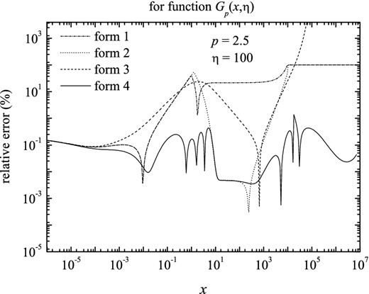
Figure 10.

The relative errors in fitting function G_p(x, η), for index p = 2.5 and η = 100, between the numerical computation of G_p(x, η) and the four approximate forms.

Open in new tab Download slide

With the latter fitting formula (i.e. the fourth form), the maximum relative error is <0.6 per cent for function G_p(x) and <5 per cent for function G_p(x, η), in the more general case (with η ≳ 3), as is reported by Fig. 11.

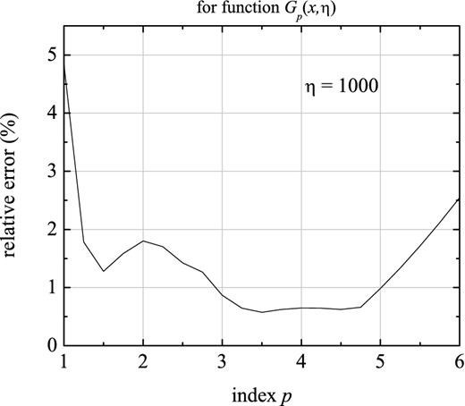
Figure 11.

The maximum relative error in fitting function G_p(x, η), versus index p, for η = 100, according to the fourth form (equations 22 and 24). It does not exceed 5 per cent, for 1 < p < 6 and η ≳ 3.

Open in new tab Download slide

5 SYNCHROTRON SELF-ABSORPTION

Absorption effects for the same population of radiating particles lead to SSA spectral shapes (Rybicki & Lightman 1979). In this case, the specific intensity is given by

\begin{equation} I_{\nu }= S_{\nu } \left( 1-{\rm e}^{-\tau _{\nu } } \right), \end{equation}

(44)

where τ_ν = α_νℓ and S_ν = j_ν/α_ν are the optical depth and the source function, respectively, expressed in terms of the absorption coefficient α_ν (with ℓ being the dimension of the radiating zone) and the emission coefficient, j_ν = P_ν/4π.

As we have shown in Fouka & Ouichaoui (2009), the absorption coefficient, α_ν = α₁α_p(x, η), and the source function, S_ν = S₁S_p(x, η), can be expressed in terms of the dimensionless functions, and α_p(x, η) and S_p(x, η), respectively, expressed in terms of function F_p(x, η) as

\begin{equation} \left\lbrace \begin{array}{ll} \displaystyle {} \alpha _{p}(x,\eta )= x^{-2}F_{p+1}(x,\eta ) \\ \displaystyle {} S_{p}(x,\eta )= \frac{F_{p}(x,\eta )}{\alpha _{p}(x,\eta )}= x^{2}\frac{F_{p}(x,\eta )}{F_{p+1}(x,\eta )} \end{array} \right., \end{equation}

(45)

where coefficients α₁ and S₁ are written as (Fouka & Ouichaoui 2009)

\begin{equation} \left\lbrace \begin{array}{ll} \alpha _{1} & = \displaystyle {} \frac{(p+2)}{8\pi m}\nu _{1}^{-2}P_{p+1}(\gamma _{1}) = P_{1}/\gamma _{1} \\ S_{1} & = \displaystyle {} \frac{P_{1}}{4\pi \alpha _{1}} = \frac{2m}{p+2}\gamma _{1}\nu _{1}^{2} \end{array} \right.. \end{equation}

(46)

Given that the two necessary quantities (α_ν and S_ν), for the computation of the SSA spectrum, are expressed explicitly in terms of function F_p(x, η), we have just to use the corresponding approximate forms to the latter, and, then, calculate α_ν and S_ν according to equation (46). However, given that the forth fitting formula for function F_p(x, η) (equation 24) is valid for values of index p within the range 1 < p < 6, then, calculation of functions α_p(x, η) and S_p(x, η) is valid for 1 < p < 5. Fig. 12 reports the absorption coefficient α_p(x, η), for index p = 2.5 and η = 100, calculated numerically and adjusted according to the four forms. Figs 13 and 14 depict the relative errors corresponding to the four proposed forms, for α_p(x, η) and S_p(x, η), respectively, with index p = 2.5 and parameter η = 100. For the absorption coefficient, α_p(x, η), the relative error reaches ∼100 per cent for frequencies x ∼ 1 and for the high-frequency range x > η², for the first and the second form, whereas for the third form it reaches ∼21 per cent for frequencies ∼0.47 and increases significantly (>100 per cent) for the high-frequency range, x > η². Indeed, in order to calculate the specific intensity for SSA spectra, the accuracy of the absorption coefficient, which is argument of the exponential function (i.e. |${\rm e}^{-\alpha _{\nu }\ell }$|⁠), is highly recommended. This constitutes a strong reason to recommend the fourth approximate form for SSA spectra, for ensuring, at least, moderate accuracy for the specific intensity. Figs 15 and 16 depict, respectively, the specific intensity, I_{ν, SSA}(x, η), and the corresponding relative errors, for index p = 2.5 and η = 100, calculated numerically and adjusted according to the four forms.

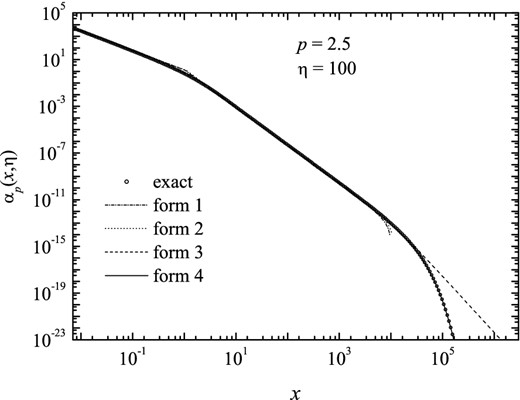
Figure 12.

The absorption coefficient, in terms of function α_p(x, η), for index p = 2.5 and η = 100, calculated numerically and adjusted according to the four forms.

Open in new tab Download slide

Figure 13.

The relative errors in fitting function α_p(x, η), for index p = 2.5 and η = 100, between the numerical computation and the four approximate forms [derived from those of function F_p(x, η)]. One remarks clearly that the fourth form [corresponding to that of function F_p(x, η); equations (22) and (24)] is the most accurate and valuable one for the whole frequency ranges. For p = 2.5, η = 100, the maximum error for the fourth form is <5 per cent.

Open in new tab Download slide

Figure 14.

The relative errors in fitting function S_p(x, η), for index p = 2.5 and η = 100, between the numerical computation and the four approximate forms [derived from those of function F_p(x, η)]. This clearly reveals that the fourth form [corresponding to that of function F_p(x, η); equations (22) and (24)] is the most accurate and valuable one for the whole frequency ranges. For p = 2.5, η = 100, the maximum error for the fourth form is <4.1 per cent.

Open in new tab Download slide

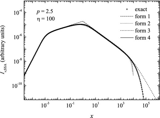
Figure 15.

The specific intensity, I_{ν, SSA}(x, η), for index p = 2.5 and η = 100, calculated numerically and adjusted according to the four forms. The latter shows a good concordance between the forth form and the exact calculation.

Open in new tab Download slide

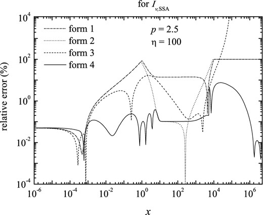
Figure 16.

The relative errors in fitting the specific intensity, I_{ν, SSA}, for index p = 2.5 and η = 100, between the numerical computation and the four approximate forms.

Open in new tab Download slide

Note that this result holds in the instantaneous (adiabatic) emission regime where cooling effects are absent or, at least, can be ignored. In this case, the particle distribution is characterized by just one index value. In contrast, the treatment is different in the case of a broken power-law particle distribution. This case is presented late in the next section.

6 CASE OF BROKEN POWER-LAW DISTRIBUTION: COOLING SPECTRA

Under conditions where the synchrotron cooling time-scale is lower than the dynamical time-scale inside the emitting region, the power-law index of radiative particles with Lorentz factor γ > γ_c (γ_c being a characteristic value differentiating between radiative and cooling particles) is increased by unity, i.e. p → p + 1. In such conditions, two situations are possible for particles with Lorentz factor γ₁ < γ < γ₂ : (i) the case γ_c < γ₁ for which all particles are radiative, called ‘fast cooling regime’ and (ii) the case γ₁ < γ_c < γ₂ for which particles with γ₁ < γ < γ_c are adiabatic and those with γ_c < γ < γ₂ are radiative, called ‘slow cooling regime’. For the first case, the particle energy distribution becomes N(γ) = C′γ^{−(p + 1)} without break, and can then be treated just with replacing index p by p + 1 in all fitting formulas presented above. Besides, for the second case corresponding to the slow cooling regime, the particle distribution takes on the form

\begin{equation} N(\gamma ) = \left\lbrace \begin{array}{ll}C_{1}\gamma ^{-p} &\quad {\rm for}\ \gamma _{1}<\gamma <\gamma _{{\rm c}} \\ C_{2}\gamma ^{-(p+1)} &\quad {\rm for}\ \gamma _{{\rm c}}<\gamma <\gamma _{2} \\ \end{array} \right., \end{equation}

(47)

with C₂ = C₁γ_c.

Then, the total spectral power can be easily deduced and is written as

\begin{equation} P_{\nu } = P_{1}F_{p}\left(\frac{\nu }{\nu _{1}},\eta _{1}\right) + P_{2}F_{p+1}\left(\frac{\nu }{\nu _{2}},\eta _{2}\right), \end{equation}

(48)

with

\begin{equation} \left\lbrace \begin{array}{ll} \displaystyle {} \eta _{1}=\frac{\gamma _{{\rm c}}}{\gamma _{1}} \ , &\quad \displaystyle {} \eta _{2}=\frac{\gamma _{2}}{\gamma _{{\rm c}}} \\ \displaystyle {} \nu _{1}=\frac{3}{2}\gamma _{1}^{2}\nu _{{\rm L}} \ , &\quad \displaystyle {} \nu _{2}=\frac{3}{2}\gamma _{{\rm c}}^{2}\nu _{{\rm L}} = \nu _{1} \eta _{1}^{2} \\ \displaystyle {} P_{1}=\frac{\pi \sqrt{3}e^{2}\nu _{{\rm L}}}{c}\gamma _{1}^{-p+1}C_{1} \ , &\quad \displaystyle {} P_{2}=\frac{\pi \sqrt{3}e^{2}\nu _{{\rm L}}}{c}\gamma _{{\rm c}}^{-p}C_{2}=P_{1} \eta _{1}^{-p+1} \end{array} \right.. \end{equation}

(49)

Then, in the case of a broken power-law particle distribution, corresponding to the slow cooling regime, the total spectral power can be written as P_ν = P₁F_p(x, η₁, η₂), with x = ν/ν₁, and function F_p(x, η₁, η₂) is written as

\begin{equation} F_{p}(x,\eta _{1},\eta _{2}) = F_{p}(x,\eta _{1})+\eta _{1}^{-p+1}F_{p+1}\left(\frac{x}{\eta _{1}^{2}},\eta _{2}\right). \end{equation}

(50)

Figs 17 and 18 depict, respectively, function F_p(x, η₁, η₂), and the corresponding relative errors, for index p = 2.5, η₁ = 100 and η₂ = 100, calculated numerically and adjusted according to the four forms.

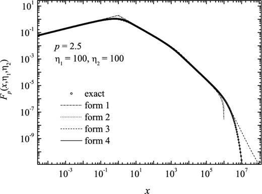
The synchrotron spectral power in the case of a broken power-law particle distribution, in terms of function Fp(x, η1, η2) defined by equation (50), for index p = 2.5 and η = 100, calculated numerically and adjusted according to the four forms. The latter shows a good concordance between the forth form and the exact calculation.

Figure 17.

The synchrotron spectral power in the case of a broken power-law particle distribution, in terms of function F_p(x, η₁, η₂) defined by equation (50), for index p = 2.5 and η = 100, calculated numerically and adjusted according to the four forms. The latter shows a good concordance between the forth form and the exact calculation.

Open in new tab Download slide

The relative errors in function Fp(x, η1, η2), in the case of broken power-law particle distribution, for index p = 2.5 and parameters η1 = 100, η2 = 100.

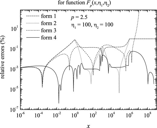
Figure 18.

The relative errors in function F_p(x, η₁, η₂), in the case of broken power-law particle distribution, for index p = 2.5 and parameters η₁ = 100, η₂ = 100.

Open in new tab Download slide

In order to calculate the SSA spectrum for a broken power-law particle distribution, we must express the absorption coefficient in its general formula, i.e. (Rybicki & Lightman 1979)

\begin{equation} \alpha _{\nu }=-\frac{1}{8\pi m\nu ^{2}} \int _{\gamma _{1}}^{\gamma _{2}} {\rm d}\gamma P(\nu ,\gamma ) \gamma ^{2} \frac{\rm{\partial} }{\rm{\partial} \gamma }\left[ \frac{N(\gamma )}{\gamma ^{2}} \right]. \end{equation}

(51)

Then, according to equation (47), one obtains

\begin{equation} \alpha _{\nu }=\alpha _{1}\alpha _{p}\left( \frac{\nu }{\nu _{1}},\eta _{1} \right)+\alpha _{2}\alpha _{p+1}\left( \frac{\nu }{\nu _{2}},\eta _{2} \right), \end{equation}

(52)

with

\begin{equation} \left\lbrace \begin{array}{ll} \displaystyle {} \alpha _{1} & = \displaystyle {} \frac{(p+2)}{8\pi m} \nu _{1}^{-2}P_{p+1}(\gamma _{1}) \\ \displaystyle {} \alpha _{2} & = \displaystyle {} \frac{(p+3)}{8\pi m} \nu _{2}^{-2}P_{p+2}(\gamma _{{\rm c}}) \\ \end{array} \right., \end{equation}

(53)

where ν_i and η_i are the same as defined in equation (49). After simplifications, the absorption coefficient can be written as α_ν = α₁α_p(x, η₁, η₂), with the extended function α_p(x, η₁, η₂) given by

\begin{equation} \alpha _{p}(x,\eta _{1},\eta _{2})= \alpha _{p}(x,\eta _{1})+ \frac{p+3}{p+2}\eta _{1}^{-(p+4)} \alpha _{p+1}\left(\frac{x}{\eta _{1}^{2}},\eta _{2}\right), \end{equation}

(54)

and, finally, the source function can be easily derived and be written as S_ν = S₁S_p(x, η₁, η₂), with S₁ = P₁/4πα₁, and function S_p(x, η₁, η₂) is written simply as

\begin{equation} S_{p}(x,\eta _{1},\eta _{2})= \frac{F_{p}(x,\eta _{1},\eta _{2})}{ \alpha _{p}(x,\eta _{1},\eta _{2}) }. \end{equation}

(55)

7 SUMMARY AND CONCLUSION

In this work, we have presented and compared four approximate formulas for the synchrotron radiation, for both optically thin and self-absorbed emission, and for both non-broken and broken power-law isotropic particle distributions. For this purpose, we have first presented a general fit formula for the instantaneous (adiabatic) synchrotron spectral power radiated by a pure power-law particle distribution with isotropic pitch angle distribution. In order to derive a more general and accurate expression, we have considered a wide range of index p values, i.e. 1 < p < 6. The central idea was to use the known asymptotic forms of the synchrotron spectral power that were multiplied by functions δ₁(x) and δ₂(x) expressed in adequate forms and depending on adjustable parameters. We have proceeded by the Levenberg–Marquardt algorithm in log–log scale in order to extract adjustable fit parameters for a given value of index p. After obtaining the adjustable parameters as functions of index p, we have generated polynomial fits of order 3 or 4 in order to account for their variations. We have shown that the relative error does not exceed 0.5 and 0.6 per cent, respectively, for functions F_p(x) and G_p(x), for the considered whole range of index p. In the general case of a particle distribution with sharp cutoff, one has to calculate function F_p(x, η) given by equation (5) in terms of function F_p(x). We have shown that according to the latter (equation 5), the relative error is increasing for frequencies x ≫ η², a problem that can be easily solved by considering the modified analytical asymptotic form (derived earlier by us) for this range. Then, we have deduced fit formulas for the degree of polarization and the SSA. We have also treated the case of cooling spectra corresponding to a particle distribution with broken power law. This has led us directly to infer the integrated spectral power, the SSA absorption coefficient and the source function with avoiding the computation of the synchrotron function, F(x) or the complementary synchrotron function G(x) and their integration under the particle distribution. We estimate that the proposed fit expressions are very useful and practical, at least for high-energy astrophysical sites involving relativistic shocks.

We would like to deeply thank the referee for his pertinent remarks and recommendations that helped us to considerably improve the content of the initial manuscript. This work was supported by the General Direction of Scientific Research and Technological Development (GDSRTD) of Algeria within the framework of the National Research Projects (NRP).

REFERENCES

Abramowitz

M.

Stegun

I. A.

,

Handbook of Mathematical Functions

,

1965

New York

Dover Press

pg.

374

Google Scholar

Google Preview

OpenURL Placeholder Text

WorldCat

Blanford

R. D.

Ostriker

J. P.

,

ApJ

,

1978

, vol.

221

pg.

L23

Crossref

Search ADS

Brainerd

J. J.

,

ApJ

,

1987

, vol.

320

pg.

714

Crossref

Search ADS

Brainerd

J. J.

Petrosian

V.

,

ApJ

,

1987

, vol.

320

pg.

703

Crossref

Search ADS

Fermi

E.

,

Phys. Rev.

,

1949

, vol.

75

pg.

1169

Crossref

Search ADS

Fouka

M.

Ouichaoui

S.

,

ApJ

,

2009

, vol.

707

pg.

278

Crossref

Search ADS

Fouka

M.

Ouichaoui

S.

,

ApJ

,

2011

, vol.

743

pg.

89

Crossref

Search ADS

Fouka

M.

Ouichaoui

S.

,

Res. Astron. Astrophys.

,

2013

, vol.

13

pg.

680

Crossref

Search ADS

Gallant

Y. A.

Guthmann

A. W.

Georganopoulos

M.

Marcowith

A.

Manolakou

K.

,

Lecture Notes in Physics, Vol. 598, Relativistic Flows in Astrophysics

,

2002

Berlin

Springer

pg.

24

Google Scholar

Google Preview

OpenURL Placeholder Text

WorldCat

Gallant

Y. A.

Achterberg

A.

,

MNRAS

,

1999

, vol.

305

pg.

L6

Crossref

Search ADS

Gallant

Y. A.

Achterberg

A.

Kirk

J. G.

Guthmann

A. W.

Kippen

R. M.

Mallozzi

R. S.

Fishman

G. J.

,

AIP Conf. Proc. Vol. 526, Gamma Ray Bursts

,

2000

New York

Am. Inst. Phys.

pg.

524

Google Scholar

Google Preview

OpenURL Placeholder Text

WorldCat

Guthmann

A. W.

Kirk

J. G.

Gallant

Y. A.

Achterberg

A.

Kippen

R. M.

Mallozzi

R. S.

Fishman

G. J.

,

AIP Conf. Proc. Vol. 526, Gamma Ray Bursts

,

2000

New York

Am. Inst. Phys.

pg.

485

Google Scholar

Google Preview

OpenURL Placeholder Text

WorldCat

Jackson

J. D.

,

Classical Electrodynamics

,

1962

New York

Wiley

Google Scholar

Google Preview

OpenURL Placeholder Text

WorldCat

Levenberg

K.

,

Q. Appl. Math.

,

1944

, vol.

4

pg.

164

Marquardt

D. W.

,

J. Soc. Ind. Appl. Math.

,

1963

, vol.

11

pg.

431

Crossref

Search ADS

Ostrowski

M.

Bednarz

J.

,

A&A

,

2002

, vol.

394

pg.

1141

Crossref

Search ADS

Petrosian

V.

Bykov

A. M.

,

Space Sci. Rev.

,

2008

, vol.

134

pg.

207

Crossref

Search ADS

Rybicki

G. B.

Lightman

A. P.

,

Radiative Processes in Astrophysics

,

1979

New York

Wiley

Google Scholar

Google Preview

OpenURL Placeholder Text

WorldCat

Sironi

L.

Spitkovsky

A.

Arons

J.

,

ApJ

,

2013

, vol.

771

pg.

54

Crossref

Search ADS

Spitkovsky

A.

,

ApJ

,

2008

, vol.

673

pg.

L39

Crossref

Search ADS

Westfold

K. C.

,

ApJ

,

1959

, vol.

130

pg.

241

Crossref

Search ADS

Download all slides

Month:	Total Views:
March 2017	3
May 2017	1
August 2017	1
September 2017	1
October 2017	5
December 2017	7
January 2018	1
February 2018	2
March 2018	7
April 2018	8
May 2018	16
June 2018	7
July 2018	11
August 2018	7
September 2018	3
October 2018	5
November 2018	3
December 2018	8
January 2019	5
February 2019	6
March 2019	10
April 2019	32
May 2019	12
June 2019	13
July 2019	7
August 2019	25
September 2019	3
October 2019	7
November 2019	16
December 2019	5
January 2020	9
February 2020	9
March 2020	13
April 2020	9
May 2020	8
June 2020	12
July 2020	2
August 2020	12
September 2020	11
October 2020	10
November 2020	14
December 2020	7
January 2021	3
February 2021	11
March 2021	17
April 2021	13
May 2021	9
June 2021	9
July 2021	8
August 2021	6
September 2021	4
October 2021	27
November 2021	4
December 2021	4
January 2022	4
February 2022	8
March 2022	8
April 2022	2
May 2022	6
June 2022	10
July 2022	7
August 2022	14
September 2022	9
October 2022	14
November 2022	22
December 2022	9
January 2023	20
February 2023	17
March 2023	10
April 2023	18
May 2023	16
June 2023	6
July 2023	7
August 2023	13
September 2023	3
October 2023	12
November 2023	10
December 2023	15
January 2024	7
February 2024	7
March 2024	14
April 2024	17
May 2024	13
June 2024	4
July 2024	7
August 2024	20
September 2024	14
October 2024	21
November 2024	16
December 2024	12
January 2025	11
February 2025	13
March 2025	22
April 2025	6
May 2025	9

Article Contents

Analytical fits for the synchrotron emission from a power-law particle distribution with a sharp cutoff

Abstract

1 INTRODUCTION

2 SYNCHROTRON POWER FROM A POWER-LAW PARTICLE DISTRIBUTION

3 ANALYTICAL FITS

3.1 The first form

3.2 The second form

3.3 The third form

3.4 The fourth form

4 DEGREE OF POLARIZATION

4.1 Approximate formulas for function G_p(x, η)

4.1.1 The first form

4.1.2 The second form

4.1.3 The third form

4.1.4 The fourth form

5 SYNCHROTRON SELF-ABSORPTION

6 CASE OF BROKEN POWER-LAW DISTRIBUTION: COOLING SPECTRA

7 SUMMARY AND CONCLUSION

REFERENCES

Citations

Views

Altmetric

Email alerts

Astrophysics Data System

Citing articles via

Latest

Most Read

Most Cited

Article Contents

Analytical fits for the synchrotron emission from a power-law particle distribution with a sharp cutoff

Abstract

1 INTRODUCTION

2 SYNCHROTRON POWER FROM A POWER-LAW PARTICLE DISTRIBUTION

3 ANALYTICAL FITS

3.1 The first form

3.2 The second form

3.3 The third form

3.4 The fourth form

4 DEGREE OF POLARIZATION

4.1 Approximate formulas for function Gp(x, η)

4.1.1 The first form

4.1.2 The second form

4.1.3 The third form

4.1.4 The fourth form

5 SYNCHROTRON SELF-ABSORPTION

6 CASE OF BROKEN POWER-LAW DISTRIBUTION: COOLING SPECTRA

7 SUMMARY AND CONCLUSION

REFERENCES

Citations

Views

Altmetric

Email alerts

Astrophysics Data System

Citing articles via

Latest

Most Read

Most Cited

This Feature Is Available To Subscribers Only

4.1 Approximate formulas for function G_p(x, η)