


Abstract
We present results from an extensive spectroscopic survey of field stars in the Small Magellanic Cloud (SMC). 3037 sources, predominantly first-ascent red giants, spread across roughly 37.5 deg2, are analysed. The line-of-sight velocity field is dominated by the projection of the orbital motion of the SMC around the Large Magellanic Cloud/Milky Way. The residuals are inconsistent with both a non-rotating spheroid and a nearly face on disc system. The current sample and previous stellar and H i kinematics can be reconciled by rotating disc models with line-of-nodes position angle Θ ≈ 120°–130°, moderate inclination (25°–70°), and rotation curves rising at 20–40 km s−1 kpc−1. The metal-poor stars exhibit a lower velocity gradient and higher velocity dispersion than the metal-rich stars. If our interpretation of the velocity patterns as bulk rotation is appropriate, then some revision to simulations of the SMC orbit is required since these are generally tuned to the SMC disc line of nodes lying in a north-east–south-west (SW) direction. Residuals show strong spatial structure indicative of non-circular motions that increase in importance with increasing distance from the SMC centre. Kinematic substructure in the north-west part of our survey area is associated with the tidal tail or Counter-Bridge predicted by simulations. Lower line-of-sight velocities towards the Wing and the larger velocities just beyond the SW end of the SMC Bar are probably associated with stellar components of the Magellanic-Bridge and Counter-Bridge, respectively. Our results reinforce the notion that the intermediate-age stellar population of the SMC is subject to substantial stripping by external forces.
1 INTRODUCTION
One of the principle goals of contemporary astrophysics is to develop a more complete understanding of galaxy formation and evolution. While the prevailing theoretical framework, Lambdacold dark matter (Λ-CDM; e.g. Peebles & Ratra 2003), is rather successful in replicating the large-scale structures observed in the Universe (e.g. Cole et al. 2005; Springel et al. 2005) it suffers significant shortcomings at explaining smaller scale phenomena where density perturbations depart strongly from the linear regime and the role of baryon physics becomes substantial (e.g. Kroupa et al. 2010; Famaey & McGaugh 2013). In Λ-CDM cosmology, galaxy formation is a hierarchical process in which the larger structures grow through the aggregation of small dark matter haloes and baryons. As the dissipative gas cools, it collapses to densities sufficient for star formation to occur (Tegmark et al. 1997). The ongoing accretion of gas with higher specific angular momentum promotes an inside-out development of galactic discs and the gradual migration in time of star formation activity to larger galactocentric radii. This is in accord with observations of negative radial chemical abundance gradients in the discs of local spiral galaxies and the formation of stars with comparatively low metallicities in their outer disc regions in the present epoch (e.g. Wang et al. 2011).
However, the basic theoretical framework overpredicts the numbers of dwarf galaxies in the local volume, including the number that are satellites to the Milky Way (MW; Klypin et al. 1999). While the mass function of galaxies might be expected to be similar in shape to that of the dark matter haloes, i.e. proportional to M−1.9, it is observed to be closer in form to M−1 in the low luminosity regime (Cole et al. 2001). In addition, observational studies of the rotation curves of dwarf galaxies show them to be slowly rising with increasing galactocentric distance (de Blok & Bosma 2002), indicative of a dark matter distribution that is significantly flatter than the centrally cusped form predicted by Λ-CDM. To account for these disparities, several mechanisms have been invoked that can both regulate the formation of stars in galaxies and smooth out the central cusp in their dark matter distributions. These include internal factors such as supernovae feedback (Governato et al. 2010), and external influences such as background UV radiation and tidal and/or ram-pressure stripping of potentially star-forming gas from a system by galaxy–galaxy interactions (Kazantzidis, Łokas & Mayer 2013). For example, observations of the Fornax galaxy cluster indicate that environmental factors regulate the levels of star formation activity in the dwarf members (Drinkwater et al. 2001).
These regulating mechanisms have also been linked to the apparently discordant outside-in progression of star formation in many low luminosity dwarf irregular systems (e.g. Zhang et al. 2012). Deep imaging studies reveal recent star formation to be concentrated within their central regions (e.g. Phoenix, IC 1613 and NGC 6822; Wyder 2001; Skillman et al. 2003; Hidalgo et al. 2009), suggesting that accretion of high angular momentum gas is inhibited. The reduction in turbulent gas pressure in the denser inner parts of these galaxies following the supernovae blow out of disc material is suspected to lead to the inward migration of enriched gas and the contraction towards their centres of the star-forming disc (e.g. Stinson et al. 2009; Pilkington et al. 2012). Additionally, tidal interactions may incite bar-like instabilities in these galaxies that can promote the inwards flow of gas in their discs.
Despite being somewhat less common than predicted by theory, dwarfs still numerically dominate the galaxy population. As the antecedents of larger galaxies such as Messier 31 and the MW, it is vital to understand their architectures and evolution, including the roles of discs rotation and pressure support, their dark matter distribution and the regulation of their star formation. The Small Magellanic Cloud (SMC) is the smaller of a pair of comparatively massive (M > 109M⊙) dwarf galaxies close (D ≤ 60 kpc) to the MW. As probable satellites of the Galaxy they are relatively unusual in that they are gas rich whereas the majority of dwarf galaxies within 270 kpc of the MW and Messier 31 appear to be gas poor (e.g. Grcevich & Putman 2009). However, there is substantial evidence that gas is being stripped from the Magellanic Clouds as a consequence of their interactions with the Galaxy and each other. For example, they are immersed within an extended body of diffuse H i gas that stretches out many tens of degrees across the sky, forming the Magellanic Stream and the Leading Arm (e.g. Putman et al. 2003).
In H i observations the SMC displays a ‘frothy’ appearance, attributed to a large number of recent supernova explosions, and a substantial velocity gradient along a position angle (PA) ≈ 60°, which has been associated with the systemic rotation of a cold disc of gas (Stanimirović, Staveley-Smith & Jones 2004). The young and the intermediate/old stellar populations of the Cloud display quite distinctive morphologies. The former have an irregular distribution and it has been inferred from observations of Cepheids that the main body of the SMC, where much of this stellar population resides, corresponds to a bar structure that is being viewed virtually end on (Caldwell & Coulson 1985). The south-west (SW) end of the main body is believed to be slightly more distant than the north-east (NE) although this latter region appears to consist of two distinct kinematic structures lying at different distances (Hatzidimitriou, Cannon & Hawkins 1993). The old/intermediate stellar population appears to be much more evenly distributed (Zaritsky et al. 2000) and recent observations suggest it extends many degrees from the centre of the Cloud (Nidever et al. 2011). Moreover, its kinematical properties appear to be consistent with those of a pressure supported spheroid (Harris & Zaritsky 2006). The contrast between the distributions of the young and the older populations has led to suggestions that the former is the outcome of a recent gas infall event (Zaritsky et al. 2000; Zaritsky & Harris 2004), while Subramanian & Subramaniam (2012) have proposed that a dwarf–dwarf merger occurred between 2 and 5 Gyr ago.
Several key observational properties of the SMC are qualitatively reproduced by N-body and chemodynamical modelling in which it interacts with the Large Magellanic Cloud (LMC) and the Galaxy, including the velocity field of the Magellanic Stream, the Magellanic-Bridge structure towards the LMC, the kinematics and the distribution of the intermediate/old stellar population, the large line-of-sight depth of the Cloud and the age–metallicity relation (Murai & Fujimoto 1980; Gardiner & Noguchi 1996; Yoshizawa & Noguchi 2003; Bekki & Chiba 2009). Realistic simulations are particularly important for reconstructing the interaction history of the Magellanic Clouds that can lead to a deeper understanding of the impact of tidal and ram pressure forces on the structure and the evolution of the SMC and dwarf galaxies in general. In addition, these computations, though accurately reproducing the properties of the Magellanic Stream, can afford further insight on the distribution of the dark matter halo of the Galaxy (Haghi, Rahvar & Hasani-Zonooz 2006).
As the initial conditions of these simulations are typically determined by integrating the Clouds’ orbits backwards in time and through choosing galaxy structures and disc orientations that lead to agreement with our understanding of the SMC in the present epoch (e.g. Gardiner & Noguchi 1996), the limitations of current observations and in our knowledge of the orbits contribute to inaccuracies in the inferred evolutionary history. Fortunately much improved proper motion determinations are becoming available and are leading to a better definition of the orbits of both the SMC and the LMC (e.g. Kallivayalil et al. 2013). Considering this, it seems timely to re-examine our understanding of the structure and kinematics of the SMC as this could also help to further refine the simulations. In this vein we have recently performed the most extensive spectroscopic study of the SMC's red giant population to date. Here we present radial velocities for in excess of 3000 stars distributed across an area of roughly 37.5 deg2 centred on the Cloud. In subsequent sections we outline our initial photometric selection of candidates and our acquisition, reduction and analysis of the spectroscopic follow-up data. We examine in detail the projected line-of-sight velocity field of the red giant population to search for evidence of large-scale trends. We compare our results to prior work on the intermediate/old and the young star populations of the SMC and consider them in the contexts of a disc model and a recent tidal interaction.
2 PHOTOMETRIC SELECTION OF CANDIDATE SMC RED GIANT STARS
An initial selection of candidate SMC red giants was made from the near-IR photometry of the 2 Micron All-Sky Survey (2MASS; Skrutskie et al. 2006) point source catalogue. A J, J − KS colour–magnitude diagram was constructed for stellar-like sources with photometric uncertainties of less than 0.5 mag in both J and KS, within an approximately 37.5 deg2 region centred on the Cloud (Fig. 1). Sources flagged as possible blends, as having photometry contaminated by image artefacts or nearby bright objects and/or as lying within the boundaries of catalogued extended sources were excluded. We selected all remaining objects to the red of the line defined by J = 26.5–20 × (J − KS) and blueward of J − KS = 2.0 or J − KS = 1.25 for 12.0 ≤ J < 13.9 and 13.9 ≤ J ≤ 15.2, respectively. These criteria, highlighted in Fig. 2, encompass the region of colour–magnitude space spanned by both the red giant branch (RGB) and asymptotic giant branch (AGB) of the SMC population and led to a preliminary catalogue of 92 893 sources.
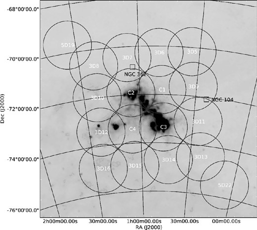
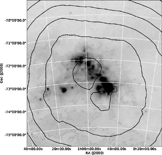
A 9° × 9° image of the sky centred on the SMC (100 μm IRIS data; Miville-Deschênes & Lagache 2005). The circles, which each corresponds to an AAT + 2dF/AAOmega pointing, highlight the areas included in our photometric and spectroscopic survey. Note that at least two distinct fibre configurations were observed for each of the four central fields. Two Galactic globular clusters within our survey area are also highlighted (open squares).
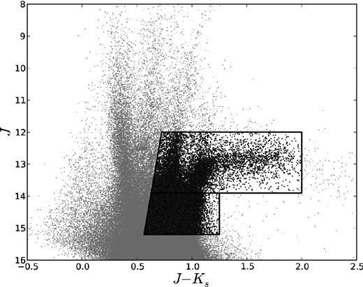
A 2MASS near-IR colour–magnitude plot of point sources in an area of roughly 37.5 deg2 towards the SMC. Sources selected for potential spectroscopic follow-up were drawn from the highlighted region.
3 OPTICAL SPECTROSCOPY
3.1 Observations and data reduction
Follow-up optical spectroscopy for a subsample of these stars was acquired during the period 2011 October 18–21, with the 2dF/AAOmega instrument and the 3.9 m Anglo-Australian Telescope (AAT) located at Siding Spring Observatory, Australia. AAOmega is a two arm fibre-fed multi-object optical spectrograph capable of the simultaneous observation of 400 objects distributed over a two degree diameter circular field of view (Saunders et al. 2004; Sharp et al. 2006).
During this observing campaign, the blue and red arms of the instrument were configured with the 1500V (R ≈ 4000) and 1700D (R ≈ 10 000) gratings and tuned to central wavelengths of 5350 and 8670 Å, respectively. This provided coverage of the λλ5167, 5172 and 5183 Å Mg b and λ8498, 8542 and 8662 Å Ca ii triplet lines. Fortunately, skies were largely clear for much of the run and seeing was generally close to the Siding Spring Observatory median value. Therefore, during the four nights approximately 7000 objects were targeted with 23 different field configurations. Details of the pointings, including dates, field centres and exposure times are reported in Table 1.
Details of the field configurations used for obtaining the spectroscopic follow-up observations of candidate SMC red giant stars.
| Name | RA | Dec. | texp | nexp | Obs. date | Plate ID | Seeing |
|---|---|---|---|---|---|---|---|
| (hh:mm:ss) | (°:′:″) | (arcsec) | |||||
| C1FA | 00:48:14 | −71:47:59 | 1200 | 3 | 2011/10/18 | 0 | 2 |
| C1FB | 00:48:14 | −71:47:55 | 1200 | 3 | 2011/10/20 | 1 | 2 |
| C2FA | 01:04:47 | −71:54:19 | 1200 | 3 | 2011/10/18 | 1 | 1.5 |
| C2FB | 01:04:47 | −71:54:25 | 1200 | 4 | 2011/10/20 | 0 | 2 |
| C3FA | 00:46:59 | −73:20:44 | 1200 | 3 | 2011/10/18 | 0 | 1 |
| C3FB | 00:47:00 | −73:20:46 | 1200 | 4 | 2011/10/20 | 1 | 1.5 |
| C3FC | 00:46:59 | −73:20:44 | 1200 | 3 | 2011/10/21 | 1 | 1.5 |
| C4FA | 01:05:00 | −73:24:27 | 1200 | 2 | 2011/10/18 | 1 | 1.5 |
| C4FB | 01:04:59 | −73:24:32 | 1200 | 3 | 2011/10/20 | 0 | 2 |
| 3D05FA | 00:33:53 | −70:10:18 | 1200 | 3 | 2011/10/21 | 0 | 1.5 |
| 3D06FA | 00:49:58 | −70:16:05 | 1200 | 4 | 2011/10/20 | 0 | 1.5 |
| 3D07FA | 01:05:50 | −70:26:53 | 1200 | 3 | 2011/10/19 | 1 | 1.5 |
| 3D08FA | 01:22:40 | −70:40:10 | 1200 | 3 | 2011/10/19 | 1 | 1.5 |
| 3D09FA | 00:31:46 | −71:36:12 | 1200 | 3 | 2011/10/19 | 0 | 2 |
| 3D10FA | 01:22:57 | −71:59:36 | 1200 | 3 | 2011/10/19 | 0 | 1.5 |
| 3D11FA | 00:27:18 | −73:01:35 | 1200 | 3 | 2011/10/18 | 0 | 2.5 |
| 3D12FA | 01:23:15 | −73:25:34 | 1200 | 3 | 2011/10/21 | 0 | 1.5 |
| 3D13FA | 00:23:34 | −74:28:10 | 1200 | 3 | 2011/10/19 | 0 | 2 |
| 3D14FA | 00:43:22 | −74:41:34 | 1200 | 3 | 2011/10/18 | 1 | 2 |
| 3D15FA | 01:04:36 | −74:55:41 | 1200 | 3 | 2011/10/21 | 1 | 1.5 |
| 3D16FA | 01:24:45 | −74:55:33 | 1200 | 3 | 2011/10/21 | 1 | 1.5 |
| 5D19 | 01:33:49 | −69:39:53 | 1200 | 3 | 2011/10/21 | 0 | 1.5 |
| 5D22 | 00:05:35 | −75:27:40 | 1200 | 3 | 2011/10/19 | 1 | 2 |
The AAOmega data were reduced using the Australian Astronomical Observatory's 2dFDR pipeline which is described at length by Bailey, Heald & Croom (2005) and Sharp & Birchall (2010). In brief, the data were first bias and dark subtracted using master frames created from exposures taken over the course of the four nights. Fibre-flat exposures of a quartz lamp, obtained immediately prior to the science observations of each target, were used to locate the spectra in each CCD frame. The fibre-flat-field and science spectra were extracted and the latter divided by the former to reduce the impact of pixel-to-pixel response variations. Spectra of a CuAr+CuNe+FeAr arc lamp, that were also acquired adjacent in time to the science observations, were then used to wavelength calibrate each data set. Finally, the multiple data sets obtained for the targets, typically three per plate configuration (see Table 1), were combined to form the final spectra.
3.2 Spectroscopic analysis
The spectra from the red arm of the instrument were first matched to multiplicative combinations of low-order polynomials and normalized synthetic spectra drawn from the library of Kirby (2011). As these models were calculated in local thermodynamic equilibrium and do not accurately reproduce the form of the strong, empirical, Ca ii triplet absorption features, the synthetic Ca lines were augmented with Voigt profiles. An iterative approach to fitting was adopted in which a χ2 goodness-of-fit statistic was minimized,1 weighting the spectral channels by their inverse variances as determined by the 2dFDR pipeline. Following this step, any points lying more than 5σ above or 3σ below the model were rejected before the data were re-fitted. This procedure was repeated three times and afforded reasonable representations of the data sets of field dwarfs and RGB stars. A useful additional outcome of this process was a model based estimate for the radial velocity of each target. Subsequently, to achieve first order normalization, each spectrum was divided by the low-order polynomial component of its corresponding model. As the synthetic spectral library employed here is not optimized for C-stars, our model representations of the spectra of objects of this nature were of lower quality but were sufficient for the purposes here.
Next, all the normalized red-arm spectra were cross-correlated with AAOmega data that we obtained for 10 RGB objects in the clusters NGC 362, Melotte 66 and NGC 288. These stars were observed through a variety of AAOmega's fibres and were adopted because reliable radial velocity estimates are available for them in the literature (Table 2). The cross-correlation procedure was undertaken with the irafFXCOR software routine running within a PyRaf environment. The quoted velocity for each star is a mean of these 10 estimates, weighted by their individual errors as reported by FXCOR. Their associated uncertainties have been determined from the mean of the absolute deviation of these measurements. As our spectroscopic sample also includes C-stars, this whole process was repeated with our AAOmega observations of six C-rich giants taken from the study of Kunkel, Irwin & Demers (1997), details of which are reported in Table 3.
Details of the 10 RGB radial velocity template stars drawn from the clusters NGC 288, NGC 362 and Melotte 66.
| ID | RA | Dec. | vr | References |
|---|---|---|---|---|
| (hh:mm:ss.ss) | (°:′:″) | (km s−1) | ||
| 403 | 00:52:46.25 | −26:37:26.0 | −46.0 | 1,2 |
| 338 | 00:52:52.80 | −26:34:38.8 | −49.2 | 1,2 |
| 344 | 00:52:52.87 | −26:35:20.2 | −49.0 | 1,2 |
| 274 | 00:53:01.13 | −26:36:07.1 | −40.5 | 1,2 |
| 2127 | 01:02:37.64 | −70:50:37.1 | +222.6 | 3,2 |
| 1441 | 01:03:21.73 | −70:48:40.4 | +222.3 | 3,2 |
| 1423 | 01:03:33.01 | −70:49:37.2 | +232.3 | 3,2 |
| 4151 | 07:26:12.07 | −47:43:24.7 | +23.0 | 4,5 |
| 4266 | 07:26:17.30 | −47:44:00.1 | +21.0 | 4,5 |
| 3133 | 07:26:30.53 | −47:41:43.9 | +18.0 | 4,5 |
Details of the six SMC C-star radial velocity templates.
| ID | RA | Dec. | vr | Reference |
|---|---|---|---|---|
| (hh:mm:ss.ss) | (°:′:″) | (km s−1) | ||
| 3D05FA 4342 | 00:21:19.5 | −70:54:36 | +139.0 | 1 |
| 3D05FA 155 | 00:26:34.3 | −70:14:24 | +158.8 | 1 |
| 3D09FA 11102 | 00:29:04.4 | −72:13:17 | +183.6 | 1 |
| 3D05FA 3280 | 00:30:47.4 | −70:28:06 | +112.6 | 1 |
| 3D05FA 2366 | 00:31:25.3 | −70:23:46 | +132.8 | 1 |
| 3D14FA 348 | 01:40:27.0 | −75:41:54 | +163.7 | 1 |
1. Kunkel et al. (1997).
3.3 Radial velocity measurements
For the vast majority of stars, the radial velocities obtained with FXCOR were found to be in excellent agreement with the values output by the χ2 model fitting procedure, above. The small number of exceptions can be attributed to spectra that are of very low signal-to-noise ratio, data sets that are severely affected by fibre fringing or spectra of C-rich stars, which we discuss later on. Nonetheless, to thoroughly assess the internal precision and external accuracy of these measurements, several further checks have been performed.
First, a small fraction of the spectroscopically observed sample (n ≈ 175) lying in overlap regions between our 2dF/AAOmega field pointings were observed twice during the course of the four night run. The different velocity estimates for these objects have been compared to each other. Excepting the handful of stars where the discrepancy appears to be much larger than typical (i.e. of the order ∼10 km s−1), a very close correspondence is observed between the two sets of measurements, with the magnitude of the velocity difference for 68 per cent of objects being Δvlos ≤ 1.9 km s−1. This scatter is comparable in size to the uncertainty estimated above.
Secondly, 17 RGB stars in the calibration cluster Melotte 66, have been observed several times previously with AAOmega by other independent teams of investigators, using different fibre configurations. These sets of measurements have been compared to each other and after excluding a probable radial velocity variable star, discussed further below, any systematic offsets between the various pairings of measurements were determined to be very small, |$\Delta v_{{\rm r}{_{\rm sys}}}$| < 1 km s−1. Additionally, the scatters in the velocity differences between our observations and those acquired on 2009 December 08, 2009 December 24 and 2011 April 22, are only 1.8, 1.7 and 1.9 km s−1, respectively, consistent with very low fibre-to-fibre velocity differences.
Thirdly, our AAOmega radial velocities for several Melotte 66 stars have been compared to recent measurements made with the European Southern Observatory's Very Large Telescope and Ultraviolet-visible echelle spectrograph (UVES), that are reported to be repeatable at the 0.5 km s−1 level (Sestito et al. 2008). While there are five objects in common with the AAOmega sample, star 1346 is one of our radial velocity templates (4266) and star 1614 is flagged as a fast rotator by Sestito et al. (2008). Together, the measurements of star 1614 suggest it is also a radial velocity variable (+17.3 ± 2.3, +17.8 ± 2.3, +25.6 ± 2.3 and +57.8±2.3 km s−1 on 2009 December 08 and 24, 2011 April 22 and October 21, respectively). For the three remaining stars the differences between the UVES and the AAOmega velocities (i.e. vAAOmega − vUVES) are only −0.42 ± 2.32 km s−1 for 1493, −0.30 ± 2.22 km s−1 for 1785 and −0.72 ± 2.36 km s−1 for 2218.
Lastly, we compared the velocity determinations for 151 SMC RGB stars common to our sample and that of Harris & Zaritsky (2006). The latter measurements are based on observations obtained with the Magellan telescope and the multislit Inamori Magellan Areal Camera (IMACS). The scatter between the sets of measurements is determined to be approximately 13.5 km s−1, which is similar in magnitude to the typical uncertainties quoted by Harris & Zaritsky (2006). However, a small systematic offset of +4.5 km s−1 (vAAOmega − vIMACS) is apparent between the results of these two studies. At face value, this seems significant but in practice it is probably not. The IMACS velocity measurements suffered from systematic errors of the order of 10 km s−1, although substantial efforts were made to mitigate these (Harris & Zaritsky 2006).
Taking stock of the results from these comparisons, we conclude that we have met our initial goal of obtaining radial velocity measurements that are repeatable to better than 5 km s−1 for the vast majority of the red giants in our sample.
3.4 C-rich stars and field dwarfs
An additional goal of this work is to investigate the metallicity of the intermediate-age population of the SMC so the primary focus of our study is the RGB star population. However, the spectroscopically observed sample includes various other stellar types too, such as field dwarfs and C-rich giants. The data obtained with the blue arm of the AAOmega spectrograph has been used to resolve these populations from each other. The 1500V data for the objects was first shifted into the rest frame using our estimates of the stellar radial velocities obtained from the red-arm spectrum during the model fitting process. A 50 Å wide section of blue arm data centred on the λλ5167, 5172 and 5183 Å Mg b lines was then cut-out and normalized. These features are known to be sensitive to surface gravity (i.e. are weaker at lower surface gravities), so their observed shapes can be exploited to separate the giants from the field dwarfs. Additionally, the energy distributions of the C-rich stars exhibit a distinctive Swan band feature at 5165 Å, so this wavelength range is useful for the discrimination of these objects too.
A set of orthogonal basis vectors was constructed to represent all the blue arm data set subsections. The principal eigenvector formed in this process (which accounts for approximately 40 per cent of the variance) can be attributed to the spectral shape induced by the strong molecular-C absorption in the atmospheres of some stars. Comparing the locations of all the spectroscopic targets and the 185 objects previously identified as C-star members of the SMC and re-observed here (Morgan & Hatzidimitriou 1995), in the 2D space defined by this new coordinate and radial velocity, the C-rich stars are observed to lie well below the locus of points de-lineated by the bulk of the sample (see Fig. 3). A by-eye inspection of the red-arm data sets for a random selection of these objects, not previously catalogued as C rich, affirms the presence of strong molecular C absorption. A 5σ clip has been applied to the main locus of points shown in Fig. 3 and the 449 objects below have been flagged as probable C-stars.

The locations of all stars in our spectroscopic sample in the 2D space defined by coordinates representing the strength of the C 5165 Å Swan band and radial velocity (grey points). Objects in our sample which have been previously identified as SMC C-rich stars are highlighted (squares). We have flagged all objects more than 5σ below the locus defined by the bulk of the sample as candidate C-stars (black points).
Subsequently, the C-stars were removed from the sample and the set of basis vectors for the remaining blue arm data was re-constructed. The principal eigenvector (corresponding to approximately 10 per cent of the variance) can now be ascribed to the λλ5167, 5172 and 5183 Å Mg b lines and the variation of their form with surface gravity. The locations of all remaining spectroscopic targets in the 2D space defined by this new coordinate and radial velocity has been compared to those of objects previously identified as red giant members of the SMC and re-observed here (Harris & Zaritsky 2006). A cursory glance at Fig. 4 reveals that the lower gravity giants are rather well separated from the field dwarfs. For example, despite having a relatively small separation in radial velocity from the field population, the RGB members of NGC 104, which encroached on one of our field configurations (3D09FA), are visible in this plot as a clump of objects at vr ≈ −15 km s−1, PC1 ≈ 0.2. The 4172 data points lying to the right of the line defined by PC1 = −0.013 vr + 1.0 (dot–dashed line in Fig. 4) and with radial velocities in the range 50 ≤ vr ≤ 250 km s−1 have been associated with probable red giant members of the SMC. Details of these objects are listed in Table 4 .

The location of all remaining stars in our spectroscopic sample in the 2D space defined by coordinates representing the strength of the λλ5167, 5172 and 5183 Å Mg b lines and radial velocity (grey points). Objects in our sample which have been previously identified as SMC RGB stars are highlighted (squares). The clump of stars at vr ≈ −15 km s−1, PC1 ≈ 0.2 corresponds to RGB stars in NGC 104 which lie in field 3D09FA. We have selected all objects lying to the right of the dot–dashed line and with radial velocities in the range 50 ≤ vr ≤ 250 km s−1 as probable red giant members of the SMC.
Details of the 4172 red giants identified in our spectroscopic follow-up of sources towards the SMC. The full table is available in the electronic version of the paper.
| RA | Dec. | 2MASS J | J | δJ | Ks | δKs | Helio. | vmodel | vhelio | δV |
|---|---|---|---|---|---|---|---|---|---|---|
| (hh:mm:ss.ss) | (°:′:″) | (mag) | (mag) | (mag) | (mag) | (corr. /km s−1) | (km s−1) | (km s−1) | (km s−1) | |
| 00:00:28.28 | −75:33:04.4 | 00002828−7533044 | 14.68 | 0.04 | 13.72 | 0.05 | 13.6 | 189.6 | 188.7 | 2.4 |
| 00:01:43.01 | −75:35:11.9 | 00014300−7535119 | 13.94 | 0.02 | 12.94 | 0.03 | 13.6 | 156.9 | 156.2 | 2.4 |
| 00:02:26.40 | −75:01:30.2 | 00022640−7501302 | 13.23 | 0.03 | 12.30 | 0.03 | 13.7 | 147.0 | 146.9 | 2.3 |
| 00:02:31.86 | −75:12:37.1 | 00023186−7512371 | 14.26 | 0.03 | 13.43 | 0.03 | 13.6 | 152.3 | 153.0 | 2.1 |
| 00:02:57.95 | −75:38:52.9 | 00025794−7538529 | 13.31 | 0.03 | 12.56 | 0.02 | 13.5 | 72.9 | 72.2 | 2.3 |
Details of the 352 carbon rich giants that were included in our spectroscopic survey of the SMC. The full table is available in the electronic version of the paper.
| RA | Dec. | 2MASS J | J | δJ | Ks | δKs | Helio. | vmodel | vhelio | δV |
|---|---|---|---|---|---|---|---|---|---|---|
| (hh:mm:ss.ss) | (°:′:″) | (mag) | (mag) | (mag) | (mag) | (corr. /km s−1) | (km s−1) | (km s−1) | (km s−1) | |
| 00:04:57.49 | −76:25:07.7 | 00045748−7625076 | 13.33 | 0.02 | 12.19 | 0.02 | 13.4 | 162.3 | 156.9 | 6.8 |
| 00:06:12.83 | −75:16:21.1 | 00061283−7516211 | 13.71 | 0.02 | 12.36 | 0.02 | 13.5 | 154.3 | 149.7 | 5.9 |
| 00:08:09.42 | −75:19:06.1 | 00080942−7519060 | 13.56 | 0.02 | 12.32 | 0.02 | 13.5 | 145.5 | 139.9 | 5.5 |
| 00:11:31.72 | −73:59:54.0 | 00113171−7359539 | 13.99 | 0.03 | 13.07 | 0.03 | 13.6 | 149.5 | 144.8 | 8.9 |
| 00:14:58.50 | −75:07:29.4 | 00145849−7507294 | 12.90 | 0.02 | 11.39 | 0.02 | 13.3 | 167.9 | 162.5 | 5.9 |
4 RADIAL VELOCITIES OF THE SMC GIANTS
4.1 The sample dominated by RGB stars
Cioni et al. (2000) determine the tip of the RGB in the SMC to lie at J ≈ 13.7 so by conservatively selecting the stars with J ≥ 14, which were not flagged as C rich in Section 3.4, we form a sample that is dominated by objects on the RGB and appropriate for a metallicity study. With radial velocities for 3037 unique RGB sources we are also in a strong position to explore the kinematics of the intermediate-age stellar population across a large swathe of the Cloud. Indeed, the Besancon model of the Galaxy (Robin et al. 2003) reveals that only 65 contaminating Galactic giants (just 2 per cent of the sample) meet our SMC RGB star colour and radial velocity selection criteria. Since a histogram of their radial velocities (Fig. 5) shows these to be relatively evenly spread across our parameter space, we conclude that they are unlikely to have any significant bearing on our subsequent analysis and conclusions.
4.2 Carbon stars
We also obtained spectroscopic data for several hundred candidate C-rich SMC giants (see Section 3.4). These objects, details of which are listed in Table 7, span the full magnitude range of our study from J = 12.0–15.2 but we have restricted our kinematic analysis to the 352 stars with J < 14.0 that are located in the canonical red AGB wing of the SMC colour–magnitude diagram (Fig. 2). Theoretical models suggest that the lowest luminosity C-rich giants may be formed in close binary systems (e.g. Marigo, Girardi & Bressan 1999). Additionally, the objects in this subsample were assigned uniformly higher priorities for spectroscopic follow-up than the stars with J > 14.0.
As discussed briefly in Section 3.4, the radial velocities of the objects flagged as C rich were determined by cross-correlating their spectra against those of six C-rich SMC giants previously investigated by Kunkel et al. (1997). These authors noted their radial velocities to be systematically shifted to the blue by about 6 km s−1 with respect to the measurements of Hardy et al. (1989). We observe an offset of similar magnitude and direction between the velocities we obtained from cross-correlation and the estimates output by our model fitting procedure. While we caution that the synthetic spectra used here were hardly ideal for matching to C-stars, we have applied an offset of +5 km s−1 to our measurements to bring them into closer agreement with both the system of Hardy et al. (1989) and our model based estimates. Following the approach taken with the RGB stars we have examined both the skew (γ1 = 0.109 ± 0.131) and the kurtosis (γ2 = −0.109 ± 0.261) of the C-star radial velocity distribution. We have found both of these parameters, together with the results of a Kolmogorov–Smirnov test (P = 0.833), to be in accord with normality (Fig. 7). We have used the maximum likelihood estimator above to determine the mean and dispersion of this distribution to be vlos ≈ 149.6 ± 1.4 km s−1 and |$\sigma _{v_{\rm los}}$| ≈ 26.1 ± 1.0 km s−1, which are in accord with the parameters of the RGB star ensemble.
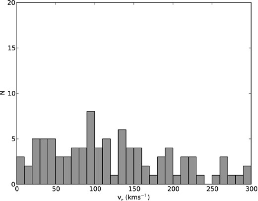
The histogram of the radial velocities of the contaminating Galactic giant stars that meet our survey selection criteria, as predicted by the Besancon model.
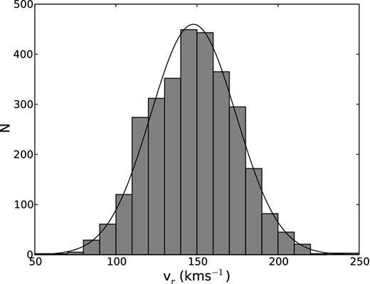
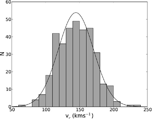
The histogram of the radial velocity estimates for our entire sample of SMC RGB stars (grey).
Histogram of the radial velocities of all C-rich stars with J < 14.0 identified in our study. The best-fitting Gaussian function to the distribution is overplotted (solid black line).
4.3 Space motion of the SMC centre of mass
To search the RGB radial velocities for evidence of systematic variation with position on sky, we have initially split the measurements up into 18 subsamples, each corresponding to a distinct 2dF field pointing. Basic parameters (e.g. the mean and the dispersion) for the radial velocity distributions of these fields have been obtained by applying the above likelihood statistic, under the assumption they too, are Gaussian. The results from this procedure are shown graphically in Fig. 8 and are listed in Table 6. These reveal an overall radial velocity gradient across the sample of about +7 km s−1 deg−1, in an approximately north-west (NW)–south-east (SE) direction. Our much smaller sample of C-stars also reflects this trend (see Fig. 9 and Table 7).
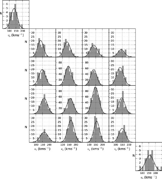
Histograms used to explore the spatial dependence of the mean radial velocity and its dispersion in our sample of SMC RGB stars. The best-fitting Gaussian function to each distribution is overplotted (solid black line).
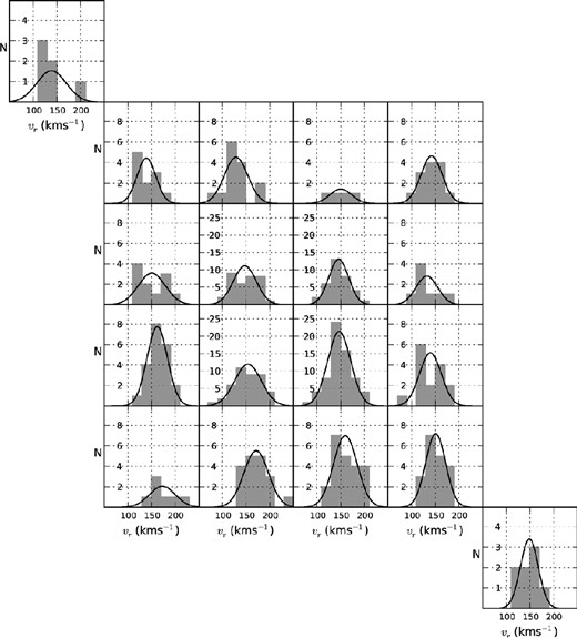
Histograms used to explore the spatial dependence of the C-star radial velocities. The best-fitting Gaussian function to each distribution is overplotted (solid black line).
Summarizing the results from fitting Gaussians to the radial velocity histograms for our spatial subsamples of RGB stars.
| Field | Ntot | vr | |$\sigma _{v_{\rm r}}$| | Δvr |
|---|---|---|---|---|
| (km s−1) | (km s−1) | (km s−1) | ||
| C1 | 321 | +135.6 ± 1.3 | 22.8 ± 0.9 | −5.4 ± 1.3 |
| C2 | 390 | +143.2 ± 1.2 | 23.2 ± 0.8 | −0.5 ± 1.1 |
| C3 | 586 | +148.6 ± 1.0 | 25.1 ± 0.8 | −0.6 ± 1.1 |
| C4 | 333 | +158.9 ± 1.4 | 24.6 ± 1.0 | +6.8 ± 1.3 |
| 3D05 | 57 | +142.2 ± 3.4 | 25.5 ± 2.4 | +16.0 ± 3.4 |
| 3D06 | 99 | +136.0 ± 2.7 | 26.8 ± 1.9 | +6.0 ± 2.8 |
| 3D07 | 112 | +134.9 ± 2.3 | 24.0 ± 1.7 | −0.7 ± 2.2 |
| 3D08 | 115 | +135.5 ± 2.1 | 22.4 ± 1.5 | −6.0 ± 2.1 |
| 3D09 | 145 | +133.8 ± 2.2 | 25.9 ± 1.6 | −1.9 ± 2.2 |
| 3D10 | 120 | +147.9 ± 2.3 | 24.7 ± 1.7 | −2.4 ± 2.2 |
| 3D11 | 121 | +145.4 ± 2.2 | 24.5 ± 1.6 | −0.1 ± 2.2 |
| 3D12 | 124 | +162.0 ± 2.3 | 25.3 ± 1.7 | +3.4 ± 2.4 |
| 3D13 | 108 | +149.5 ± 2.4 | 25.0 ± 1.7 | −3.1 ± 2.4 |
| 3D14 | 142 | +157.3 ± 1.8 | 21.7 ± 1.3 | −0.0 ± 1.8 |
| 3D15 | 170 | +163.8 ± 1.9 | 24.9 ± 1.4 | +2.1 ± 1.9 |
| 3D16 | 92 | +162.6 ± 3.1 | 29.2 ± 2.2 | −4.8 ± 3.1 |
| 5D19 | 29 | +136.3 ± 4.4 | 23.4 ± 3.2 | −2.3 ± 4.5 |
| 5D22 | 29 | +156.1 ± 5.7 | 30.3 ± 4.1 | −0.4 ± 5.6 |
Summarizing the results from fitting Gaussians to the radial velocity histograms for our spatial subsamples of C-stars.
| Field | Ntot | vr | |$\sigma _{v_{\rm r}}$| | Δvr |
|---|---|---|---|---|
| (km s−1) | (km s−1) | (km s−1) | ||
| C1 | 34 | +145.7 ± 3.7 | 20.8 ± 2.8 | +2.9 ± 3.7 |
| C2 | 34 | +147.3 ± 4.3 | 24.3 ± 3.2 | +1.3 ± 4.3 |
| C3 | 65 | +146.7 ± 3.1 | 24.2 ± 2.3 | −2.4 ± 3.0 |
| C4 | 42 | +154.0 ± 4.4 | 28.0 ± 3.2 | +2.3 ± 4.3 |
| 3D05 | 13 | +141.8 ± 6.6 | 22.4 ± 4.8 | +15.4 ± 6.9 |
| 3D06 | 4 | +150.0 ± 12.5 | 22.6 ± 6.7 | +17.8 ± 14.3 |
| 3D07 | 14 | +128.8 ± 6.9 | 24.7 ± 5.1 | −7.0 ± 6.4 |
| 3D08 | 11 | +139.3 ± 6.4 | 19.8 ± 4.7 | −2.9 ± 7.3 |
| 3D09 | 8 | +132.0 ± 8.6 | 22.8 ± 6.4 | −5.6 ± 8.4 |
| 3D10 | 11 | +150.7 ± 9.0 | 28.5 ± 6.5 | +1.0 ± 8.9 |
| 3D11 | 15 | +139.5 ± 6.3 | 23.1 ± 4.6 | −5.8 ± 6.2 |
| 3D12 | 21 | +162.3 ± 5.0 | 21.6 ± 3.7 | +4.7 ± 5.1 |
| 3D13 | 19 | +150.6 ± 5.1 | 21.1 ± 3.8 | +0.0 ± 5.1 |
| 3D14 | 22 | +159.7 ± 5.6 | 25.1 ± 4.0 | +5.0 ± 5.5 |
| 3D15 | 18 | +171.4 ± 6.4 | 26.0 ± 4.7 | +10.9 ± 6.1 |
| 3D16 | 7 | +173.0 ± 10.9 | 27.2 ± 8.0 | +5.8 ± 11.2 |
| 5D19 | 6 | +138.7 ± 13.5 | 31.2 ± 7.5 | −2.2 ± 14.6 |
| 5D22 | 8 | +148.7 ± 7.2 | 18.8 ± 5.3 | −7.7 ± 7.0 |
As discussed by previous investigators (e.g. van der Marel et al. 2002), a substantial contribution to our observed radial velocity gradient may stem from the expected variation in the line-of-sight velocity component of the Cloud's space velocity across our extensive survey area. A number of estimates of the proper motion of the SMC centre of mass have been published since the RGB star study of Harris & Zaritsky (2006) and these have substantially reduced uncertainties compared to similar earlier work. The most recent is based on three epochs of Hubble Space Telescope (HST) imaging and has measured μαcosδ = 0.772 ± 0.063 mas yr−1 and μδ = −1.117 ± 0.061 mas yr−1 (Kallivayalil et al. 2013). We have used this information in conjunction with a kinematical model for solid body rotation (e.g. van der Marel et al. 2002) to assess the impact of the Cloud's tangential motion on our measured values. We have neglected for now any contribution to the velocities from a putative disc structure, and, for consistency with the work of Kallivayalil et al. (2013), we have assumed initially that the SMC centre of mass is coincident with the H i kinematic centre (Stanimirović et al. 2004). This model was matched to the measured radial velocities of the individual RGB stars by locating the global minimum of a χ2 goodness-of-fit statistic. We allowed the model parameters vsys, vt and Θt [in the notation of van der Marel et al. (2002), respectively, the systemic velocity, the tangential velocity and the PA of the tangential velocity, east (E) from north(N)] to vary freely in this process. We assumed for now an intrinsic velocity dispersion of |$\sigma _{v_{\rm los}}$| = 25 km s−1, which is compatible with both the typical values we measure for the subsamples across the cluster and the results of earlier studies of the intermediate-age stellar population of the Cloud.
We find this basic model can provide a reasonable match to the data with a reduced-χ2 ≈ 1 for parameter values of vsys = 147.5 ± 0.5 km s−1, vt = 416.8 ± 23.0 km s−1 and Θt = 152|$_{.}^{\circ}$|1 ± 2|$_{.}^{\circ}$|9. The errors quoted here were obtained via a bootstrap with random replacement approach. The broad agreement between these parameters and the values inferred from the most recent estimate of the SMC centre-of-mass proper motion, vt = 386 ± 21 km s−1 and Θt = 145|$_{.}^{\circ}$|4 ± 2|$_{.}^{\circ}$|6 (assuming a distance modulus of (m−M)0 = 18.90) and our determination of the radial velocity, vsys = 147.7 ± 0.5 km s−1, argues that any manifestation of systemic rotational motion in the RGB star kinematics has an amplitude well below the velocity dispersion of this population.
4.4 Main trends in the velocity field of the red giant sample
To reveal any more subtle velocity structures within our data set, the predictions of our basic kinematical model have been subtracted from our measurements. Subsequently, we constructed a surface of the velocities in the rest frame of the SMC galaxy (GRF) for our survey area by estimating this parameter at a series of regularly spaced grid points in RA and declination (every 10 arcmin), using a bi-variate Gaussian smoothing kernel, with an adaptive width corresponding to one third the distance to the 200th closest star, to weight the individual measurements (e.g. Walker et al. 2006b). A contour plot of this surface is displayed in Fig. 10 and a map of the width of the smoothing kernel is shown in Fig. 11. No gradient in the red giant velocity field is obvious along the major axis of the SMC Bar. This is consistent with the results of most previous kinematical studies of the intermediate and old populations of the SMC. For example, Dopita et al. (1985) reported a lack of organized structure in the velocities of 44 planetary nebulae located largely along the Bar, while both Hatzidimitriou et al. (1997) and Hardy et al. (1989) found no evidence of systemic rotation in their radial velocities of modest sized samples of C-stars.
A 6|$_{.}^{\circ}$|0 × 6|$_{.}^{\circ}$|5 contour map of the RGB star galaxy rest-frame velocity surface after subtraction of a solid body model of the centre-of-mass proper motion of the SMC (see the text for details). The velocity data around each grid point were smoothed using an adaptive Gaussian kernel with a width corresponding to one third of the distance to the 200th closest star. The contours correspond to steps of 4 km s−1 (heavy line 0.0 km s−1, dashed lines negative velocities).
A 6|$_{.}^{\circ}$|0 × 6|$_{.}^{\circ}$|5 map of the width of the smoothing kernel used to produce Fig. 10. The contours correspond to steps of 10 arcmin, where the inner most contour corresponds to 10 arcmin.
Nonetheless, Fig. 10 reveals a rather striking dipole-like velocity pattern within roughly the central 10 deg2 that has a major axis almost perpendicular to the SMC Bar. To the NW side of the Bar, negative GRF velocities at v < −5 km s−1 predominate, while immediately to the SE, positive velocities extend to v > +10 km s−1. An analysis of several thousand simulated velocity data sets, which were generated by randomly re-assigning the GRF velocities to the positions of our sample stars, indicates that this signal is statistically significant (Fig. 12). The implied velocity gradient here is similar in magnitude and direction to that induced by the transverse motion of the Cloud centre of mass as estimated recently from proper motion measurements of the inner regions of the SMC. This gradient could be largely accounted for if these astrometric measurements were systematically underestimated by at least 50 per cent in both RA and declination. However, while the most recent determination of the transverse motion of the Cloud is smaller than most previous estimates, the reduction does not amount to 50 per cent, so it seems unlikely that the observed effect is due to grossly inaccurate astrometry.
A 6|$_{.}^{\circ}$|0 × 6|$_{.}^{\circ}$|5 contour map of the statistical likelihood that the features in the galaxy rest-frame velocity surface are not merely due to chance (P = 0.95–0.99 in light grey, P = 0.99–0.999 in grey and P > 0.999 in dark grey).
Hardy et al. (1989) measured a larger mean velocity (160.7 ± 5.6 km s−1) for a sample of C-stars which they ascribed to the SMC Wing but their field appears to be coincident with one of the zones of positive GRF velocity indicated by the red giant stars, adjacent to the SE edge of the bar. A contour plot of the velocity surface derived from our sample of several hundred C-stars (constructed following the above procedure) has a broadly similar pattern to the corresponding RGB star map but hints at larger velocities much further out in the Wing region towards the eastern limit of our survey (Fig. 13).
A 6|$_{.}^{\circ}$|0 × 6|$_{.}^{\circ}$|5 contour map of the carbon star GRF velocity surface after subtraction of a solid body model of the centre-of-mass proper motion of the SMC. Other details of this plot are the same as in Fig. 10.
In contrast to our work, Harris & Zaritsky (2006) found evidence of a velocity gradient of +8.3 km s−1 deg−1 at PA ≈ 23°, E of N, in their investigation of 2046 red giants drawn from 12 fields located mainly around the SMC Bar. Given the apparent discrepancy between their result and that of the present work, we have explored their conclusion further. Considering the somewhat limited extent of their survey in the NW–SE direction, it is conceivable that a comparatively shallow gradient along this axis may have been concealed by their larger measurement uncertainties. Alternatively, the PA may have been incorrectly referenced (e.g. from due E, rather than due N), with the value quoted by Harris & Zaritsky (2006) perhaps in error by −90°. We have re-evaluated the direction of the steepest velocity gradient in our RGB ensemble using a subsample of 1038 stars from roughly the same region of sky as the Harris & Zaritsky (2006) objects. We have added random velocity offsets, drawn from a Gaussian distribution with a mean of 0.0 km s−1 and a width of 10 km s−1, to our measurements to ensure that the uncertainties for stars in the two samples have similar magnitudes. Subsequently, we have calculated half the difference between the mean velocities of our red giant stars on either side of a line bi-secting the subsample, through the optical centre of the Cloud, stepping the PA of this line in 10° increments from 0° to 360° (e.g. Mackey et al. 2013). This entire process was repeated 100 times and, despite the smaller sample size, in every case the parameters of the resulting velocity curve were consistent with the steepest gradient lying along an approximately NW to SE direction (peak amplitude of between 4–6 km s−1 and a PA at the maximum differential velocity in the range PA ≈ 25°–45°). Next, we applied the above procedure to their 2046 stars and found the differential velocity curve to have a peak amplitude of approximately 6 km s−1 and a PA at the maximum value of PA ≈ 45°. The broad agreement between the values obtained from their data set and ours suggests that the likely explanation for the disparity between the two results is that the PA quoted in Harris & Zaritsky (2006) was inadvertently referenced from E.
Our contour plot of the RGB star velocity surface also reveals a sizeable kinematic structure towards the NW of our survey area, where GRF velocities reach values of v > +10 km s−1. This region appears linked to the positive velocities SE of the central SMC via the southern end of the Bar. In the prominent eastern, Wing region of the Cloud, the velocity field displays no overwhelming trend. The lack of a strong, positive signal in the NE zone of our RGB star velocity field contrasts with the findings of kinematical studies of the H i gas (e.g. Stanimirović et al. 2004), which were taken to be indicative of systemic rotation around the minor axis of the Bar. In fact, there is a substantial pool of low velocities further to the NE, which is also evident as a secondary peak (centred on the 115–130 km s−1 bin) in the histograms for fields 3D7, 3D8 and 3D10 (e.g. see Fig. 8). De Propris et al. (2010) have also noted the velocity distribution of the RGB stars to the E (and the south) of the SMC centre to be bi-modal, but their reported peaks are at approximately 160 km s−1 and 200 km s−1, somewhat larger than the values we observe. This region of our survey encompasses a small sample of red clump stars spectroscopically examined by Hatzidimitriou et al. (1997) and with which they identified a positive correlation between velocity and distance. Nidever et al. (2013) have recently identified two relatively distinctive intermediate-age stellar structures, in terms of distance (approximately 55 kpc and 67 kpc), projected several degrees to the E and N of the Cloud.
4.5 Old/intermediate versus young stellar population
To gain further insight, we have compared our results to those from another large-scale 2dF based kinematical study of the stellar population of the Cloud. Evans & Howarth (2008) observed 2045 massive stars and also identified a trend of increasing radial velocity from NW to SE, across the bar. It was concluded that this velocity gradient of approximately +25 km s−1deg−1 at a PA ≈ 126° could not be attributed solely to variation in the viewing angle of the SMC's centre-of-mass motion. In accord with earlier investigations (e.g. Maurice et al. 1987), they found the stars in the Wing to have significantly larger velocities than those of the Bar (vlos ≈ 195 km s−1). Interestingly, most of the objects in this region turned out to be amongst the earliest spectral types surveyed in their work (i.e. O and early B), which concurs with the finding of Cignoni et al. (2013) that there has been a substantial increase in the rate of star formation here within the last 200 Myr. However, the majority of the later-type supergiants that were observed concentrate in two main elongated aggregates to the west of α = 01h12m, one extending NE–SW along the Bar (W) and the other, from the NE end of the Bar, south along α = 01h05m (E) (Fig. 14). The 2dF spectroscopic fibre allocation process could conceivably have led to some apparent differences in the spatial distributions of these massive star populations but there is some evidence of the E aggregate in a density isopleth contour plot for SMC stars with ages in the range 0.1 Gyr < τ < 0.3 Gyr and 0.3 < τ < 1 Gyr. This structure is not apparent in the corresponding plot for the youngest objects with τ < 0.1 Gyr (fig. 4 of Belcheva et al. 2011). There are also hints of this bi-modality in the spatial distribution of SMC star clusters with ages less than 3.5 Gyr (e.g. fig. 15 of Rafelski & Zaritsky 2005).
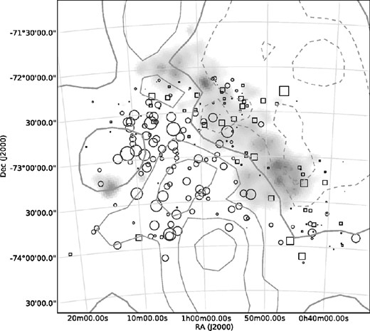
A 3|$_{.}^{\circ}$|5 × 3|$_{.}^{\circ}$|5 zoom-in on Fig. 10. The entire F/G supergiant sample from Evans & Howarth (2008) is overplotted with those stars having positive GRF velocities represented as circles and those with negative velocities shown as squares. The size of the symbols scale linearly with the magnitude of the residuals, the NW and W most stars having −83 km s−1 and +55 km s−1, respectively. The division of negative and positive F/G supergiant velocities follows closely the zero contour delineated by the RGB stars.
Evans & Howarth (2008) advised that their 2dF based velocity measurements were likely to be marginally overestimated (by a mean of +10 km s−1). The results of our examination (i.e. cross-matching with the catalogues of Ardeberg & Maurice 1979; Maurice et al. 1987; Mathewson, Ford & Visvanathan 1988) point to a systematic error that is somewhat dependent on spectral type. While it may be as large as +20 km s−1 for the O and early B objects, it appears to be smaller than +10 km s−1 for the latest stars in the study. Consequently, in performing a direct comparison between the radial velocities of our red giants and the massive stars, we have worked with only their F/G supergiants. After considering, as above, the relative space motion of the Cloud's centre of mass, we determine that these two aggregates of massive stars, E and W as discussed above, are dominated by positive and negative GRF velocities, respectively. These groupings appear to loosely correspond to the location and sign of the main velocity zones we observe in the RGB star velocity map (Fig. 14). Fig. 15 shows the differences in the mean radial velocities of both the F/G supergiants and a subsample of our red giant stars, drawn from roughly the same region of sky, on either side of a bi-secting line that passes through the optical centre of the Cloud, (α = 00h53m, δ = −72°50′; de Vaucouleurs & Freeman 1972), as a function of this line's PA. The sinusoidal-like forms of these curves have distinct amplitudes (Δ < vr > max ≈ 16 km s−1 and Δ < vr > max ≈ 4.5 km s−1) but have very similar phases (PA ≈ 26° and 30°). This conclusion is not changed significantly if, like Evans & Howarth (2008), we had adopted α = 01h00m, δ = −73°00′ as the centre. The inferred velocity gradients perpendicular to these PAs are +20.0 ± 0.8 and +6.1 ± 0.1 km s−1 deg−1 for the F/G supergiants and the red giant stars, respectively. The former can easily account for the small slope of +6.5 km s−1 deg−1 measured in the F/G star GRF velocities along a PA ≈ 60°, the direction of the steepest velocity gradient observed in the H i gas (Stanimirović et al. 2004). It also appears plausible that the slope of +10 km s−1deg−1 along this direction reported by Evans & Howarth (2008) is merely a manifestation of the gradient they identified along a PA ≈ 126°.
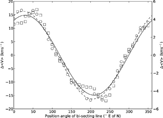
The differences in the mean radial velocities of the F/G supergiant (circles; scaling on left-hand axis) and RGB (squares; scaling on right-hand axis) star samples on either side of a bi-secting line passing through α = 00h53m, δ = −72°50′, as a function of PA. The best-fitting sinusoids to these data are overplotted (F/G supergiants, dashed line and RGB stars, solid line).
Despite some marked differences between the kinematics of the intermediate/old and the massive stellar populations in the SMC (e.g. the lack of an obvious Wing related structure in the complete red giant sample), there appear to be several similarities (e.g. both display a velocity gradient along a NW–SE direction). We emphasize here that H i maps of the Cloud also provide some weak evidence of a velocity gradient extending from NW to SE, at least across the southern portion of the Bar (see fig. 5 of Stanimirović et al. 2004).
5 INTERPRETATION AND DISCUSSION
5.1 Systemic rotational motion?
We have split our red giant sample into quartiles on the basis of their metallicities. Considering the form of the SMC age–metallicity relation and its relative invariance across the galaxy (e.g. Noël et al. 2009; Piatti 2012; Cignoni et al. 2013), this is effectively a subdivision of the stellar population in age, with the more metal-rich stars typically being significantly younger (e.g. Dobbie et al. 2014). The metallicity of each red giant was determined from measurements of the equivalent widths of the Ca ii triplet lines and full details of this process are provided elsewhere (Dobbie et al. 2014). Subsequently, we have undertaken a comparison of the kinematics of the upper and the lower quartiles ([Fe/H] > −0.86 and [Fe/H] < −1.15, respectively) to gain greater understanding of the structure of the SMC. For each subsample we have constructed a contour plot of the radial velocities remaining after accounting for the centre-of-mass motion of the Cloud (Figs 16 and 17). We have also determined the line-of-sight velocity and dispersion profiles of these subsamples and the F/G supergiants, along a line through the optical centre at PA = 120°, which we found in Section 4.5 aligned with the maximum velocity gradient (Fig. 18). The latter population shows substantial changes in velocity along this axis, reaching approximately +30 km s−1 at the south-eastern limit of the Evans & Howarth survey coverage (corresponding to a projected distance from the SMC centre of approximately 1 kpc). Away from the north-western limit of our survey region (discussed further below), our metal-poor and presumed older red giants display a line-of-sight velocity profile that is effectively flat (χ2 = 7.9 for 9 d.o.f.). The line-of-sight velocity profile of our metal-rich and generally younger red giant subsample displays a significant gradient, albeit less pronounced than that of the F/G supergiants, reaching 8–10 km s−1, 1–1.5 kpc from the centre. Considering that it is a combination of random and systemic rotational motions of stars around a galaxy which act to balance the gravitational potential of the system, it is interesting that these latter stars also have a significantly smaller mean line-of-sight velocity dispersion, |$\sigma _{v_{\rm los}}$| ≈ 22.3 ± 0.6 km s−1, than the older metal-poor red giants, |$\sigma _{v_{\rm los}}$| ≈ 26.1 ± 0.7 km s−1 (at angular distances > −1|$_{.}^{\circ}$|5). As stars age, repeated gravitational encounters increase the random component of their mean velocities (e.g. Binney & Tremaine 2008). The increased velocity dispersion and lower apparent rotation velocity of the metal-poor RGB stars relative to the metal-rich portion of the sample supports the contention that an age–metallicity relation exists in the SMC.
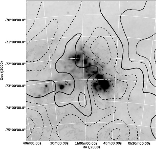
A 6|$_{.}^{\circ}$|0 × 6|$_{.}^{\circ}$|5 contour map of the GRF velocity surface for the lowest metallicity quartile of our red giant star sample after subtraction of a solid body model of the centre-of-mass proper motion of the SMC. Other details of this plot are the same as in Fig. 10.
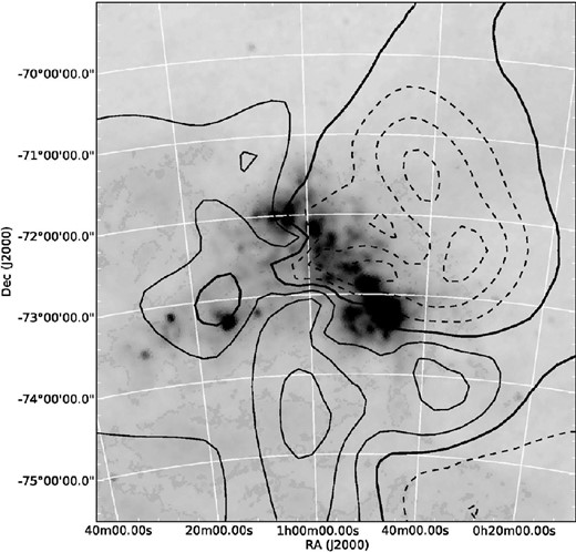
A 6|$_{.}^{\circ}$|0 × 6|$_{.}^{\circ}$|5 contour map of the GRF velocity surface for the highest metallicity quartile of our red giant star sample after subtraction of a solid body model of the centre-of-mass motion of the SMC. Other details of this plot are the same as in Fig. 10.
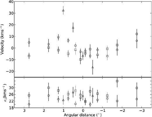
Velocity (upper) and velocity dispersion (lower) profiles along PA = 120° for the metal-poor red giants (squares), metal-rich red giants (circles) and the F/G supergiants (triangles).
The inferred gradient of 30–35 km s−1deg−1 in the F/G star population is comparable in magnitude to that predicted by the Bekki & Chiba (2009) simulations of the SMC/LMC/Galaxy interaction, although it is significantly less than anticipated by the N-body calculations of Gardiner & Noguchi (1996). The intermediate and old stellar populations are also anticipated to display a velocity gradient but the models attribute this largely to streaming motions along the tidal structures of the Cloud (e.g. Diaz & Bekki 2012). However, it is not immediately obvious why our two subsamples display different line-of-sight velocity profiles since strong tidal forces from an interaction with the LMC (or the Galaxy) within the last few 100 Myr would have presumably affected all our intermediate-age red giant stars.
In view of the coincidence of the PAs of the velocity gradients in our red giant and the F/G supergiant samples and our observation that the generally younger red giants with greater metallicities exhibit a larger systemic motion and a lower mean velocity dispersion, we conjecture that the velocity pattern we detect is related to systemic rotation of disc-like structure. This notion is supported by the intriguing alignment of the Cloud's coherent magnetic field almost perpendicular to the Bar, as mapped through the polarization of radio continuum emission and optical starlight (e.g. Mathewson & Ford 1970; Mao et al. 2008). The magnetic fields of both the Galaxy and the LMC are observed to trace the spiral structure of their discs. Wayte (1990) previously concluded from his analysis of the SMC magnetic field that the Bar is not a true bar structure and instead, interaction with the LMC prompted an extension of the Cloud towards the NE and the formation of the Wing.
5.2 Modelling the velocities as a putative SMC disc
To investigate the above possibility, we have attempted to replicate the measured radial velocities of the metal-rich red giant stars by adding a disc component to the kinematical model of Section 4.3, following the formalism of van der Marel et al. (2002). This time we have assumed a distance to the SMC of 60 kpc and adopted a tangential velocity of vt = 386 km s−1 at PA Θt = 145|$_{.}^{\circ}$|4 as derived from the most recent Kallivayalil et al. (2013) centre-of-mass proper motion measurement. We have also initially fixed the inclination angle of our disc component at i = 5°, which is comparable to that determined by Subramanian & Subramaniam (2012) and Haschke, Grebel & Duffau (2012) from the distribution of the red clump and RR Lyrae members of the Cloud and adopted the optical determination of the centre. In lieu of the results of the previous section, we have also assumed a somewhat smaller intrinsic line-of-sight velocity dispersion of |$\sigma _{v_{\rm los}}$| = 22.3 km s−1. This model was matched to the observations by locating the global minimum of a χ2 goodness-of-fit statistic, allowing the parameters Θ, R0, η, V0, |$\frac{{\rm d}i}{{\rm d}t}$| and vsys (following the notation of van der Marel et al., respectively, the PA of the line of nodes, E of N, the disc velocity scaling radius, disc velocity scaling index, maximum disc velocity, the rate of change of the disc inclination angle and the systemic velocity) to vary freely. Our best-fitting model representation of the data, with parameters Θ = 127° ± 9°, R0 = 0.04 ± 0.04 kpc, η = 3.69 ± 0.9, V0 = 91 ± 11 km s−1, |$\frac{\rm{d}i}{\rm{d}t}$| = 0.48 ± 0.19 mas yr−1 and vsys = 148.3 ± 0.8 km s−1, has a χ2 = 778.2 for 760 degrees of freedom (the uncertainties were determined using a bootstrap with random replacement approach). The corresponding model without a disc component has a χ2 = 824.9 for 765 d.o.f.
Considering the distribution of the F-statistic for ν1 = 5 and ν2 = 760, we find the addition of the disc component to the kinematic model provides a significant improvement to our reproduction of the observations. However, empirical studies of low luminosity, late-type systems have highlighted that their rotation curves attain lower circular velocities than those of more massive galaxies (e.g. Rubin et al. 1985; Broeils 1992; Swaters et al. 2009). With an integrated apparent B magnitude of 2.58 ± 0.07 mag (Bothun & Thompson 1988), a distance of 60 kpc and B−R = 1 mag (Swaters 1999), we estimate the absolute R magnitude of the SMC to be only MR ≈ −17.3 mag and anticipate the circular velocity of the cold H i disc to reach only Vc ≈ 60–70 km s−1 several disc scalelengths from the centre. While these latter values are comparable to the velocities determined at the limits of the H i study of Stanimirović et al. (2004), they are substantially less than those delineated by the rotation curve of our virtually face on disc model, even before any allowance is made for the asymmetric drift velocity of the red giant population. Moreover, our estimate of V0 is even larger if we adopt instead the H i centre as the kinematic centre.
We have performed a rough assessment of the asymmetric drift by noting that for an inclination angle of i = 5°, the observed velocity dispersion is effectively σz, the vertical component in the disc. Adopting the disc geometry from the fit above, we have determined the radial gradient of the spatial density of stars in the SMC (v) by modelling the azimuthally averaged brightness profile of the galaxy as measured from 3.36 μm WISE imaging (Wright et al. 2010). We used a function of the form |$v = v_{0}\exp (\frac{-R}{R_{\rm exp}})$|, where the exponential scalelength, Rexp, is found to have a value of 0.76 ± 0.08 kpc. Subsequently, assuming that in the putative SMC disc σz ≈ 0.7σR ≈ σϕ (the latter two variables represent the radial and azimuthal components of the disc velocity dispersion, respectively), which Hunter et al. (2005) argue to be appropriate at least for spiral galaxies (e.g. NGC 488, the MW), we have followed Hinz, Rix & Bernstein (2001) to estimate the asymmetric drift velocity ranges from 22 km s−1 at 0.75 kpc to 55 km s−1 at 2.75 kpc. In light of these sizeable corrections, it appears quite unlikely that the velocity signature we observe in the red giant stars can be attributed to a disc that is viewed at a low inclination angle. This conclusion is independent of the parametrization of the disc rotation curve.
Needless to say, we can obtain plausible values for the circular velocity of the disc if the inclination angle is assumed to be larger. For example, with i ≈ 60°, which is comparable to inclination estimates derived from the younger stellar populations in the Cloud (e.g. Haschke et al. 2012; Laney & Stobie 1986), the best-fitting disc model has V0 ≈ 20 km s−1 (with Θ = 122°, R0 ≈ 8.7 kpc, η ≈ 0.01, |$\frac{{\rm d}i}{{\rm d}t}$| ≈ 0.5 mas yr−1 and vsys ≈ 148 km s−1). The initial rise of this parametrized rotation curve is rather abrupt and seemingly unphysical. However, the asymmetric drift velocity of the RGB star population beyond the inner few 100 pc is substantial and renders the raw rotation curve, which we are modelling, effectively flat at all larger disc radii. To explore alternative inclination angles further, we have also probed the red giant line-of-sight velocities with a tilted ring model (Begemann 1987). For this part of the investigation we have adopted six radius intervals with width 0.5 kpc from 0.0–3.0 kpc and have fixed the inclination angle at i = 25°, which is similar to that estimated in the pioneering study of the SMC by de Vaucouleurs (1955) and intermediate to the values discussed above. We have also anchored the kinematic centre and the rate of change of the inclination angle at the values preferred from our analysis above. The line-of-nodes PA and the velocity of each ring were permitted to vary freely in the fitting process. The results, both raw and after accounting for the generally substantial asymmetric drift velocity, are shown in Fig. 19, where for the latter, we have taken |$\sigma _{v_{\rm los}}\approx \sigma _{\phi }$| (e.g. Hunter et al. 2005).
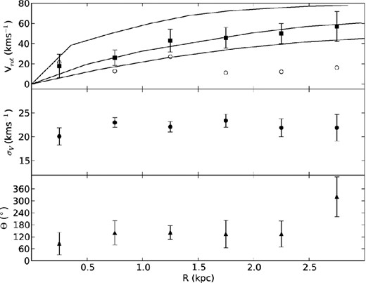
Velocities (top, open circles), velocity dispersions (middle, filled circles) and line-of-nodes PAs (lower, filled triangles) from our tilted ring analysis of the metal-rich red giant sample. Estimates of the circular velocity of the putative SMC disc, accounting for asymmetric drift, are also shown (top, filled squares). The H i rotation curves of several dwarf galaxies e.g. UGC 7603 (middle curve), UGC 7971 (bottom curve) and UGC 8490 (upper curve), are also overplotted in the top panel.
At this assumed inclination angle, the inferred rotation curve rises relatively swiftly to 20 km s−1 and continues to increase gradually to approximately 50 km s−1 at a radial distance of 2–2.5 kpc. Within the significant uncertainties, it is comparable to the empirical data for other low luminosity, gas-rich systems which almost invariably show a slow, steady rise in circular velocity with increasing galactocentric distance that generally continues to the outermost measurement point (e.g. UGC 7603, UGC 7971, UGC 8490; Swaters et al. 2009). It is also similar to the H i disc velocities measured for the dwarf irregular NGC 6822, which rise to Vc ≈ 50 km s−1 around 3 kpc from the centre (Weldrake, de Blok & Walter 2003). This dark matter dominated galaxy is similar in luminosity (MB ≈ −15.8) to the SMC but has a much lower velocity dispersion. The line-of-sight velocity dispersion of the SMC red giants is effectively constant with galactocentric distance, with no evidence for a decrease towards larger radii as anticipated for a disc embedded in a dark halo (σv ∝ R−1). A mild positive correlation between radial distance and the velocity dispersion of the carbon stars several kpc out in the LMC has been attributed to disc flaring (Alves & Nelson 2000).
The impact of systemic rotation with a magnitude of V ≈ 25 km s−1 at an inclination angle of 25° on estimates of the SMC centre-of-mass tangential velocity is only a few per cent and within the uncertainties that propagate from the HST proper motion measurements of (e.g. μdisc ≲ 0.04 mas yr−1; Kallivayalil et al. 2013). Given the locations of their five proper motion measurements, the details of this minor effect are heavily dependent on the position of the disc rotation centre. For example, if this corresponds to the optical centre, then the contribution of the systemic motion is predominantly in a SE direction, so the current centre-of-mass tangential velocity determination will be slightly overestimated. Conversely, if the H i centre represents the stellar rotation centre then the disc component to the tangential motion is predominantly in a N/NW direction, resulting in a slight underestimate of the centre-of-mass tangential velocity. The effect of systemic rotation is even smaller if the disc is being viewed at a larger inclination angle e.g. i ≈ 60°.
We note that the PA inferred for the disc line of nodes changes abruptly by around 180° at a projected galactocentric distance of approximately 2.5 kpc. This might have been anticipated from an inspection of Fig. 10, which reveals a large region of generally positive velocities towards the far WNW of our survey region (higher velocities are also evident in this region in the RGB star radial velocity study of De Propris et al. 2010). If the red giant stars here are also part of a disc structure in the same plane, then they appear to be counter-rotating with respect to the inner 2–3 kpc of the SMC. Alternatively, these objects might compose a disc rotating in a similar sense to the inner regions that is merely viewed at a quite different inclination angle. However, counter-rotation of gas has been observed in other irregular galaxies such as NGC 4448 and IC 10 (e.g. Hunter et al. 1998). The latter object is a slightly less luminous (MB ≈ −15.5) cousin of the SMC that has recently entered an epoch of intense star formation (Wilcots & Miller 1998). The gas in its central regions displays a modest rotational signature, peaking at 30–35 km s−1, but at galactocentric distances greater than 1–2 kpc there are several H i structures with velocities that run counter to expectations based on the continuation of the kinematic trends of the inner galaxy. Wilcots & Miller (1998) have suggested that IC 10 may have recently accreted this material from an extended reservoir, leading to the current burst of star formation.
The accretion of a gas rich dwarf galaxy has been invoked by several investigators (e.g. Zaritsky et al. 2000; Rafelski & Zaritsky 2005; Bekki 2008; Subramanian & Subramaniam 2012) to account for the stark differences in the morphologies of the SMC's young and older stellar populations and/or the substantial variations in the Cloud's star formation rate within the last few Gyr. However, as discussed further in Dobbie et al. (2014), recent theoretical exploration of the chemical evolution of the SMC, which treats a major gas rich accretion event, anticipates a fairly pronounced dip in the age/metallicity relation (Tsujimoto & Bekki 2009) for which there is little support from recent empirical determinations that consider both star clusters and field stars (Piatti 2011, 2012). Additionally, studies of the LMC indicate it has experienced substantial increases in star formation activity at similar times to the SMC (e.g. Smecker-Hane et al. 2002; Harris & Zaritsky 2009), disfavouring a triggering mechanism that was specific to the evolutionary history of the latter. Considering this and given the proximity of the SMC to the LMC and the Galaxy, their history of tidal interaction and the results of N-body simulations within the literature, in the next section we discuss another explanation, which we consider more likely, for these apparently counter-rotating stars.
5.3 Tidal speculation
The larger the galactocentric distance of a star, the more susceptible it typically is to being dislodged by the forces which arise in a galaxy–galaxy interaction (e.g. Mihos & Hernquist 1994). A two-sample Kolmogorov–Smirnov test on the normalized cumulative radial distributions for the upper and the lower metallicity quartiles of our red giants (constructed by adopting the semi-major axis of an ellipse, with a/b = 1.5 and an origin at the centre of the Cloud, on which a star lies, as a proxy for its galactocentric distance; e.g. Piatti et al. 2007; Subramanian & Subramaniam 2012) confirms that the spatial distributions of these subpopulations are significantly different. The metal-poor quartile displays a considerably more extended distribution, in accord with the detection by Carrera et al. (2008) of a radial metallicity gradient in the SMC field red giants. The kinematic structure towards the NW limits of our survey region, which is weakly evident in our C-star velocity surface and in H i surveys of the Cloud (e.g. fig. 5 of Stanimirović et al. 2004), is most apparent in the data for our metal-poor RGB star subsample (e.g. Figs 16–18).
Bekki & Chiba (2009) predict an extension in the surface density of the intermediate/old stellar SMC populations towards the NW (their fig. 6), which they attribute to prior interaction with the LMC and/or the Galaxy. According to the simulations of Gardiner & Noguchi (1996), a tidal tail formed by the most recent encounter with the LMC, extends from the main body of the galaxy, initially in a broadly south-westerly direction, before turning back towards the NE, behind the Cloud. This structure appears to be analogous to the gaseous ‘Counter-Bridge’ of the more recent modelling of Diaz & Bekki (2012), that similarly is predicted to extend out behind the SMC. Both the Magellanic-Bridge and the Counter-Bridge are expected to display a positive correlation between velocity and distance (e.g. Gardiner & Noguchi 1996), which, at least in the former case, appears to have empirical support. For example, the closer of the two relatively distinctive structures identified by Nidever et al. (2013) towards the N and E of the main body, which they propose to be an intermediate-age stellar counterpart of the Magellanic-Bridge, is associated with a secondary, lower velocity component observed in this direction (e.g. Hatzidimitriou et al. 1997, and our Fig. 8).
Our velocity histograms towards the W and NW of the Cloud, fields 3D5, 3D9 and 3D11, suggest a secondary, higher velocity peak here (170–180 km s−1) but it is considerably less well populated than the low velocity structure on the NE side. Nidever et al. find no compelling evidence of multiple stellar populations along the lines of sight towards their W and NW pointings, although the peak in the distance distribution of the red clump stars in their field 40S296 is at a marginally greater distance (approximately 71 kpc) than that in the bulk of their other samples. The neighbouring pointings 40S251 and 40S206, despite their lower overall populations, also hint at somewhat more distant stars. Despite a lack of detailed agreement in terms of the projected spatial distribution of these structures, between observations and the results of the simulations of the interaction of the SMC, LMC and Galaxy, in consideration, we find tidal formation of this apparently counter-rotating, kinematical structure towards the NW to be preferred over a galaxy merger/accretion origin. Consequently, we propose these stars are a stellar component of the ‘Counter-Bridge’ tidal tail. Our finding that the higher velocity peak towards the NW is much weaker than the low velocity structure on the NE side, concurs with the predictions of a recent maximum interaction simulation of the Magellanic system. While models in which the Clouds merely experience a close encounter (e.g. Besla et al. 2012; Diaz & Bekki 2012, model 1) appear to show the Bridge and the Counter-Bridge have comparable stellar densities, the latter is postulated to be considerably less well populated than the former in a simulation involving a direct collision between the LMC and SMC around 100 Myr ago (Besla et al. 2012). A very strong interaction between the Clouds seems necessary to account for the sizeable observed population of SMC AGB stars that have been accreted on to the LMC (Olsen et al. 2011).
The influence of tidal forces on the SMC could also be a plausible explanation for the moderate rate of change of the inclination angle we infer for the putative disc in our modelling of the line-of-sight velocities of the centrally concentrated metal-rich red giants (|$\frac{{\rm d}i}{{\rm d}t}$| ≈ 140° Gyr−1). Piatek & Pryor (1995) have demonstrated using an N-body simulation of a dwarf spheroidal interacting with a larger galaxy that the effects of tidal forces can be manifest as an apparent rotation around the minor axis of the satellite. However, it is not clear if the viewing geometry here is conducive to this. These simulations also indicate that stars residing at smaller galactocentric radii are dislodged in a galaxy–galaxy interaction since an additional factor which dictates their fates is velocity along the line-of-centres (Piatek & Pryor 1995). While the changing inclination of the LMC's disc has been attributed to the impact of tidal torques from the Galaxy van der Marel et al. (2002), further investigation of the SMC kinematics indicates that the non-negligible value of |$\frac{{\rm d}i}{{\rm d}t}$| here stems from the protrusion of lower velocities towards the Wing region, lower velocities towards the NE of our survey area and an excess of positive stellar GRF velocities just beyond the SW end of the SMC Bar (see Fig. 17). The two zones of negative GRF velocities, at least, appear to tie in with features previously touted as having formed as a result of the most recent encounter with the LMC. In view of the kinematics and the locations of the stars towards the Wing and around the SW end of the Bar it is tempting to associate them with, respectively, the lower velocity foreground complex proposed by Nidever et al. (2013) as an intermediate-age stellar component of the Magellanic-Bridge and the structure in the W and NW of our survey area that we have advanced as a stellar analogue of the ‘Counter-Bridge’. However, the signs of the velocities in both regions appear to be contrary to expectations from simulations of the SMCs evolution (e.g. Diaz & Bekki 2012; Gardiner & Noguchi 1996). Perhaps at least part of this discrepancy is due to an incorrect assumption in these calculations of the orientation of the SMC stellar disc. Nonetheless, these new observations and prior theoretical and empirical studies (e.g. Bekki & Chiba 2009; Olsen et al. 2011) paint a complex picture of an intermediate-age stellar population in the SMC that is subject to substantial tidal stripping. Given the expected distances between the SMC and MW compared to the SMC–LMC separation over the past 3–5 Gyr, the magnitude of the tidal force of the LMC on the SMC may have been more than an order of magnitude higher than the MW–SMC tidal force. It is not unreasonable to link the SMC structure and history to its orbit around the LMC rather than the MW.
6 SUMMARY
We have acquired optical spectroscopy for a sample of 3037 predominantly RGB stars distributed across 37.5 deg2 of the SMC and have measured their radial velocities to an accuracy of better than 5 km s−1. The main results of our analysis of these data sets, as illustrated in Fig. 20, are as follows.
We have found a velocity gradient in the rest frame of the SMC which is consistent in phase with that observed in the young, massive stellar population by Evans & Howarth (2008). The line-of-sight velocity and velocity dispersion profiles for the most metal-poor giants, the most metal-rich red giants and the F/G supergiants, along a PA ≈ 120°, the direction of the steepest gradient, and the arrangement of the Cloud's coherent magnetic field across the Bar suggest this arises from the systemic rotation of disc structure.
The orientation of this putative stellar disc is discordant with the PA of the SMC kinematic axis derived from H i observations (PA ≈ 60°). This inconsistency is challenging considering that the F/G supergiants examined here would have had only circa 200 Myr in which to dynamically separate from the H i gas. The source of the discrepancy may be due to degeneracies in the model formalism for linear (or nearly linear) rotation curves (see below).
An almost face-on viewing angle (i ≈ 5°) has been favoured by recent studies of the intermediate and old stellar populations of the SMC. Analyses of the line-of-sight velocity of the most metal-rich SMC red giant stars, following the disc formalism of van der Marel et al. (2002) and with a tilted ring model, show that for such low inclinations the inferred circular velocities (Vc ≳ 90 km s−1) are much larger than those typically observed in a galaxy of the SMC's luminosity (Vc ≈ 60–70 km s−1). It is thus unlikely that the velocity patterns seen in these stars are attributable to a disc viewed nearly face-on.
Assuming a larger inclination angle (e.g. i ≈ 25°), comparable to that determined by de Vaucouleurs (1955), we can infer a rotation curve for an SMC disc that, within the uncertainties of our analysis, is accordant with those of similarly luminous galaxies such as NGC 6822. If a disc with a kinematic major axis along a PA ≈ 120° is the correct interpretation of the observed velocity patterns within the central regions of our survey area then some revision to simulations of the evolution of the Cloud may be required as these are generally tuned to the disc plane lying in a NE–SW direction at the present epoch. However, the neglect of this systemic rotation has only a minor impact on estimates of the Cloud's centre-of-mass tangential motion.
Considering the proximity of the SMC to the LMC and the Galaxy, their history of tidal interaction and the different spatial distributions of the young and old stars within the Cloud, we associate a kinematical structure towards the far NW of our survey area, that is particularly evident in the velocities of our most metal-poor red giants, with the tidal ‘Counter-Bridge’ tail predicted by N-body and hydrodynamical simulations of the SMCs most recent interaction with the LMC.
The moderate rate of change of the disc inclination angle, |$\frac{{\rm d}i}{{\rm d}t}$| ≈ 140° Gyr−1, inferred by our modelling, is also likely attributable to the influence of tidal forces on the SMC. The protrusion of lower velocities towards the Wing region and an excess of positive stellar GRF velocities just beyond the SW end of the SMC Bar, observed in kinematics of the younger, metal-rich RGB stars, are probably associated with a lower velocity foreground complex proposed by Nidever et al. (2013) as an intermediate-age stellar component of the Magellanic-Bridge and the structure in the W and NW of our survey area that we advance as a stellar analogue of the ‘Counter-Bridge’, respectively.
The disagreement between disc parameters derived from H i and stellar velocities opens the question of how to appropriately model a system in which multiple processes contribute similar amounts to the observed velocities. For example, the inferred rate of change of inclination of the H i disc of about 400° Gyr−1 (Indu & Subramaniam, in preparation) is much larger than that for the stellar disc and represents a radial velocity gradient of approximately 5.5 km s−1 kpc−1 along the major axis of the disc. This is of the same order as the apparent velocity gradient induced by the transverse motion of the centre of mass, and not much smaller than the disc rotation velocities we derive. The |$\frac{{\rm d}i}{{\rm d}t}$| and Vc contributions are defined to be perpendicular to each other, and so model algorithms are likely to trade one against the other when the rotation curve is linear. In the SMC case, we also have to consider that the proper motion is directed nearly parallel to the stellar disc PA. This degeneracy is likely to be broken only when significant samples of stars beyond the radius at which the rotation curve flattens out are measured, and the data considered in the light of the origins of any torques that could significantly alter the disc angular momentum.
A more spatially extensive radial velocity survey of the young stellar population, including sources located N of the δ = −72° limit of the Evans & Howarth work, would help address questions relating to the putative SMC disc structure we have tentatively identified from the kinematics of the youngest red giant stars in our sample. A spectroscopic survey of the SMC's red giant population at larger projected galactocentric distances than included by our survey area would also be useful to search for a continuation (or otherwise) of kinematic trends identified here and would provide greater insight on the existence and extent of the tidal structures.
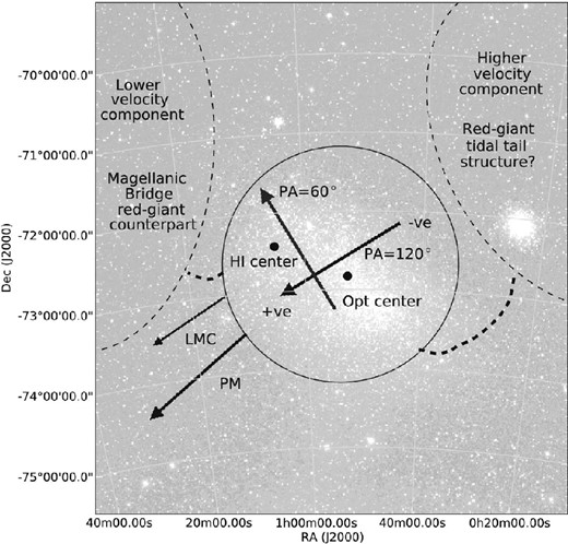
A conceptual plot of the SMC highlighting the PAs of the H i (Stanimirović et al. 2004) and the RGB star kinematic axes (this work). The locations of the NE (possibly the Magellanic-Bridge) and the suspected NW (possibly the ‘Counter-Bridge’) tidal structures are highlighted, as are the optical and the H i centres of the Cloud, the SMC's direction of tangential motion and direction of the LMC.
This paper makes use of data products from the Two Micron All Sky Survey, which is a joint project of the University of Massachusetts and the Infrared Processing and Analysis Center/California Institute of Technology, funded by the National Aeronautics and Space Administration and the National Science Foundation. This research was supported under the Australian Government's Australia-India Strategic Research funding scheme (reference number ST040124).
REFERENCES
SUPPORTING INFORMATION
Additional Supporting Information may be found in the online version of this article:
Table 4. Details of the 4172 red giants identified in our spectroscopic follow-up of sources towards the SMC.
Table 5. Details of the 352 carbon rich giants that were included in our spectroscopic survey of the SMC (Supplementary Data).
Please note: Oxford University Press are not responsible for the content or functionality of any supporting materials supplied by the authors. Any queries (other than missing material) should be directed to the corresponding author for the paper.
