


Abstract
We present a simple formula for the Hamiltonian in terms of the actions for spherically symmetric, scale-free potentials. The Hamiltonian is a power law or logarithmic function of a linear combination of the actions. Our expression reduces to the well-known results for the familiar cases of the harmonic oscillator and the Kepler potential. For other power laws, as well as for the singular isothermal sphere, it is exact for the radial and circular orbits, and very accurate for general orbits. Numerical tests show that the errors are always very small, with mean errors across a grid of actions always <1 per cent and maximum errors <2.5 per cent. Simple first-order corrections can reduce mean errors to <0.6 per cent and maximum errors to <1 per cent. We use our new result to show that: (1) the misalignment angle between debris in a stream and a progenitor is always very nearly zero in spherical scale-free potentials, demonstrating that streams can sometimes be well approximated by orbits, (2) the effects of an adiabatic change in the stellar density profile in the inner region of a galaxy weaken any existing 1/r dark matter density cusp, which is reduced to 1/r1/3. More generally, we derive the full range of adiabatic cusp transformations and show that a |$1/r^{\gamma _0}$| density cusp may be changed to |$1/r^{\gamma _1}$| only if γ0/(4 − γ0) ≤ γ1 ≤ (9 − 2γ0)/(4 − γ0). It follows that adiabatic transformations can never completely erase a dark matter cusp.
1 INTRODUCTION
The benefit of action–angles extends beyond their simple time evolution, however. Despite the fact that galaxies are never truly in a steady state, equilibrium models are hugely important tools in developing our understanding of galaxies. Using equilibrium models, we can infer the gravitational potential of a galaxy and predict all observable quantities. Under most circumstances, we are justified in assuming that a galaxy is always close to an equilibrium state, and we can model non-equilibrium effects such as accretion or stellar evolution as small perturbations to the system.
Given the assumption of dynamical equilibrium, the most efficient way to proceed is via the use of the Jeans theorem (see Binney & Tremaine 2008), which tells us that the phase-space distribution function (hereafter DF) of a galaxy or stellar system in equilibrium may be written as a function of just three isolating integrals. This reduces the dimensionality of the space under consideration from six to three, and so invoking the Jeans theorem leads to an elegant simplification of the modelling problem. Since actions are adiabatic invariants, if we choose to write the DF as a function of the actions, its functional form is preserved under slow changes to the galaxy. This property can be exploited to model various processes in galaxy evolution. For example, Goodman & Binney (1984) showed that the adiabatic growth of mass at the centre of a stellar system causes the velocity dispersion to become tangentially distended, a process invoked by Agnello et al. (2014) to explain the kinematics of M87's globular cluster populations. Similarly, Katz et al. (2014) recently modelled the adiabatic compression of dark matter haloes in galaxies from the THINGS survey to reproduce their rotation curves. Another example is provided by Gondolo & Silk (1999), who showed that the adiabatic growth of a black hole can cause a dark matter spike at the centre of a cusped dark halo.
Unfortunately, although action–angles are very useful when known, they are not usually available analytically. In fact, Evans, de Zeeuw & Lynden-Bell (1990) showed that the most general potential in which the actions are available as elementary functions is the isochrone (which reduces to the Kepler and harmonic potentials in limiting cases). Recent efforts by Binney (2012), Bovy (2014) and Sanders & Binney (2014) mean that actions can now be numerically recovered in many potentials, but analytical approximations are still sparse. Though numerical methods are ultimately the most widely applicable, analytical approximations are important in so far as they give us valuable insight into the properties of a system, not to mention drastically reduced computational time when they are sufficiently accurate.
In this paper, we present a new method for finding accurate approximations to the Hamiltonians of spherically symmetric, scale-free systems and apply it to general power-law potentials and the isothermal sphere. We then use the method in two applications: finding the misalignment angle of a stellar stream, and calculating the effect of a slowly changing central stellar density profile on the slope of a dark matter cusp.
2 METHOD
If our Hamiltonian is not scale free, we can often break the problem up into scale-free regimes, and devise an interpolation formula that smoothly matches the limits. A specific example of this is provided by Evans & Williams (2014), who provided a Hamiltonian |$\mathcal {H}(L,J_r)$| for a halo model with a 1/r density cusp at the centre but a flat rotation curve at large radii.
3 POWER-LAW POTENTIALS
3.1 Results
So, we have found a surprisingly simple and compact formula (12) for the Hamiltonian in terms of the actions valid for any power-law potential with −1 ≤ α ≤ 2. It is exact for the two classical cases – the Kepler potential and the harmonic oscillator – which have been known for over a century. Note too that the frequencies Ωi are rationally related only in the case of the Kepler potential and the harmonic oscillator. Thus, we have recovered Bertrand's theorem (see e.g. Goldstein 1980), which states that the only central force laws with everywhere closed bound orbits are the linear and inverse square force laws. For all other cases, our formula (12) gives frequencies that are incommensurable and so the motion is conditionally periodic.
3.2 Errors and first-order corrections
Given that the approximation is only exact for the cases α = −1 and α = 2, we tested the effectiveness of the approximation for several values of α: −0.5, 0 (the isothermal sphere), 0.5, 1 and 1.5. In each case, we evaluate a set of 10 000 orbits on a grid of pericentre and apocentre radii: rp = 0 → 50, ra = 0 → 100. For each orbit, we evaluate the energy and angular momentum, which are available as algebraic expressions in terms of pericentre and apocentre radii (Lynden-Bell 2010), and the radial action, which requires the evaluation of a numerical integral. This results in an irregularly spaced grid in action space.
We find that the errors in all cases are very small. The mean absolute percentage error on the action grid is <1 per cent in every case, and the maximum absolute percentage error is always < 2.5 per cent. These results are given in Fig. 1. The distribution of errors is very similar in all cases: it is scale free and maximized along a particular ray in action space. A typical example is given in Fig. 2.
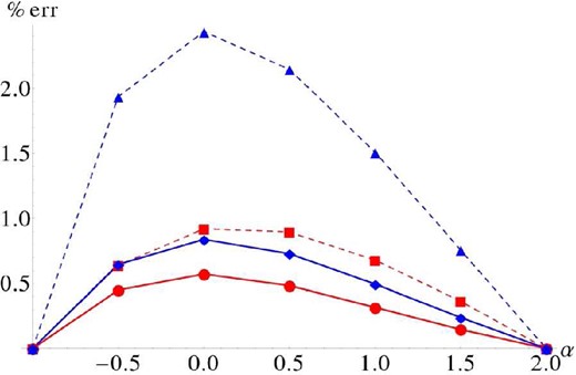
Absolute percentage errors against power-law index (α = 0 corresponds to the isothermal sphere). The dashed lines correspond to the original approximation, and the solid lines include first-order corrections. Blue lines are maximum absolute percentage errors across the action grid, red lines are the mean absolute percentage errors. One can see that the first-order corrections reduce the maximum error significantly, and also have a noticeable effect on the mean error.
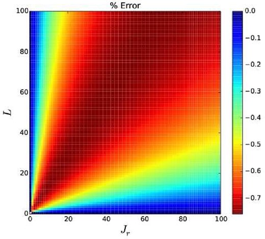
Distribution of percentage error with actions for the case α = 1.5. One can see a definite systematic trend that could be removed with an astute choice of first-order correction.
4 APPLICATIONS
Here, we present two simple applications of our results. The first is to stellar streams. We demonstrate that within this approximation streams are well delineated by orbits. The second is to cusps in the centre of galaxies. We show that the central slope of a dark matter halo is reduced when the stellar populations begin to dominate the potential.
4.1 Stellar streams
4.2 Adiabatic transformation of density cusps
Navarro et al. (1996) famously discovered that, in dissipationless simulations, dark haloes form a 1/r density cusp in the centre of galaxies. However, there is a discrepancy between the predicted density of dark matter at the centre of spiral galaxies and the inferred dark matter density consistent with observations. For example, in the case of the Milky Way, Binney & Evans (2001) show that cuspy dark matter density haloes would violate constraints on the rotation curve, given the known contributions from the stellar and ISM discs and Galactic bar. Clearly, the 1/r cusp, if it originally formed in the Milky Way galaxy, has been weakened with the passage of time.
We assume that the dark halo of the galaxy formed first, and that the dark matter density in the centre of a galaxy originally followed a 1/r cusp. With the build-up of the disc and bulge stellar populations, we assume that the density profile of the dominant stellar populations becomes roughly constant in the very central parts. In this instance, the potential is initially linear (α0 = 1), corresponding to the NFW cusp, and becomes harmonic, (α1 = 2), corresponding to a constant density core. Assuming that this process occurs sufficiently slowly that the adiabatic invariance of the actions holds good, then we can find the final profile of the dark matter.

The domain of allowed cusp slope transformations. The final cusp slope γ1 is plotted against the initial cusp slope γ0. Shaded regions cannot be reached by adiabatic changes. The upper line corresponds to γ1(γ0, −1) (the Keplerian limit) and the lower line to γ1(γ0, 2) (the harmonic limit).
Finally, we note that Gondolo & Silk (1999), in their study of the response of a dark matter cusp to a growing black hole, derived the limit γ1(γ0, −1), though only for models with 0 < γ0 < 2. The formula is generally valid throughout the entire physical range 0 ≤ γ0 ≤ 3, though the methods employed by Gondolo & Silk (1999) were unable to include isothermal cusp slopes and steeper.
5 CONCLUSIONS
Action–angle coordinates are a powerful tool in modern classical mechanics (see e.g. Abraham & Marsden 1978; Arnold 1989) and galactic dynamics (Binney & Tremaine 2008). Their widespread use is hampered by the fact that the actions can be difficult to find explicitly. Although numerical tools are becoming available to make this job easier (Binney 2012; Bovy 2014; Sanders & Binney 2014), there are disappointingly few potentials for which analytic results are possible.
The main result of the paper is the discovery of a simple formula for the Hamiltonian of scale-free potentials in terms of the actions. The formula recovers the well-known and exact results for the harmonic oscillator and Keplerian potentials, which have been known for over a century (see e.g. Goldstein 1980). For other power laws, the formula is exact for radial and circular orbits, but approximate for general orbits. However, numerical tests show that the errors are always very small, with mean errors across a grid of actions always <1 per cent, and maximum errors never larger than 2.5 per cent. Our formula therefore provides a useful and accurate approximate Hamiltonian for many of the commonly used galactic potentials, including the isothermal sphere and power-law cusps. It may also be improved with simple first-order corrections if need be, which reduce the mean error to always <0.6 per cent, and the maximum error <1 per cent.
We provided two applications. First, the mismatch of streams from their progenitor is described by a misalignment angle. This in turn is controlled by the Hessian of the Hamiltonian with respect to the actions (Sanders & Binney 2013). Most streams in the Milky Way halo occur at Galactocentric radii greater than 20 kpc, so that the potential is probably scale free to a good approximation. If, in addition, the potential is nearly spherical, then we have shown that the misalignment angle must be close to zero. This suggests that there are regimes in which the approximation of thin streams by orbits may be a reasonable one.
Secondly, we considered the evolution of a dark matter 1/r density cusp in a spiral galaxy. Although 1/r density cusps are known to be the endpoint of dissipationless simulations, there is ample evidence that in galaxies like the Milky Way, any such cusp must have been modified at the centre (Binney & Evans 2001). The response of a 1/r cusp to the slow build-up of a stellar bulge and disc can be computed using our formula, under the assumption of adiabatic invariance. As the overall potential becomes cored and harmonic, the dark matter density cusp becomes shallower and is nearly erased. It began as a 1/r and finished as 1/r1/3 density cusp. Considering the more general problem of density cusps of arbitrary slope, we show that adiabatic transformations can only weaken, and never remove, such cusps. A density singularity – once present – requires some non-adiabatic process to erase it.
In this paper, we only considered scale-free potentials. Nonetheless, our methods can also be applied to spherical potentials that possess a scalelength. This requires more work because we have to devise a suitable interpolation scheme to sew the different regimes together, but it is still very effective. Evans & Williams (2014) provide a specific example, but it would be interesting to study this problem in greater generality.
We thank Donald Lynden-Bell and Simon Gibbons for some extremely useful conversations and insights. AW and AB acknowledge the support of STFC.
