


Abstract
Observations of molecular gas in high-z star-forming galaxies typically rely on emission from CO lines arising from states with rotational quantum numbers J > 1. Converting these observations to an estimate of the CO J = 1-0 intensity, and thus inferring H2 gas masses, requires knowledge of the CO excitation ladder or spectral line energy distribution (SLED). The few available multi-J CO observations of galaxies show a very broad range of SLEDs, even at fixed galaxy mass and star formation rate (SFR), making the conversion to J = 1-0 emission and hence molecular gas mass highly uncertain. Here, we combine numerical simulations of disc galaxies and galaxy mergers with molecular line radiative transfer calculations to develop a model for the physical parameters that drive variations in CO SLEDs in galaxies. An essential feature of our model is a fully self-consistent computation of the molecular gas temperature and excitation structure. We find that, while the shape of the SLED is ultimately determined by difficult-to-observe quantities such as the gas density, temperature and optical depth distributions, all of these quantities are well correlated with the galaxy's mean star formation rate surface density (ΣSFR), which is observable. We use this result to develop a model for the CO SLED in terms of ΣSFR, and show that this model quantitatively reproduces the SLEDs of galaxies over a dynamic range of ∼200 in SFR surface density, at redshifts from z = 0 to 6. This model should make it possible to significantly reduce the uncertainty in deducing molecular gas masses from observations of high-J CO emission.
1 INTRODUCTION
Stars form in giant clouds in galaxies, comprised principally of molecular hydrogen, H2. Due to its low mass, H2 requires temperatures of ∼500 K to excite the first quadrapole line, while giant molecular clouds (GMCs) in quiescent galaxies have typical temperatures of ∼10 K (e.g. Fukui & Kawamura 2010; Dobbs et al. 2013; Krumholz 2014). The relatively low abundance of emitting H2 in molecular clouds has driven the use of the ground-state rotational transition of carbon monoxide, 12CO (hereafter CO), as the most commonly observed tracer molecule of H2. With a typical abundance of ∼1.5 × 10⁻⁴ × H2 at solar metallicity, CO is the second most abundant molecule in clouds (Lee, Bettens & Herbst 1996). Via a (highly debated) conversion factor from CO luminosities to H2 gas masses, observations of the J = 1-0 transition of CO provide measurements of molecular gas masses, surface densities and gas fractions in galaxies at both low and high redshifts.
CO can be excited to higher rotational states via a combination of collisions with H2 and He, as well as through radiative absorptions. When the CO is thermalized, then level populations can be described by Boltzmann statistics, and the intensity at a given level follows the Planck function at that frequency.
While the conversion factor from CO luminosities to H2 gas masses is based solely on the J = 1-0 transition, directly detecting the ground state of CO at high z is challenging. Only a handful of facilities operate at long enough wavelengths to detect the redshifted 2.6 mm CO J = 1-0 line, and consequently the bulk of CO detections at high redshift are limited to high-J transitions (see the compendia in recent reviews by Solomon & Vanden Bout 2005; Carilli & Walter 2013). Thus, to arrive at an H2 gas mass, one must first down-convert from the observed high-J CO line intensity to a J = 1-0 intensity before applying a CO–H2 conversion factor. This requires some assumption of the CO excitation ladder, or as it is often monikered in the literature, the spectral line energy distribution (SLED).
Typically, line ratios between a high-J line and the J = 1-0 line are assumed based on either an assumption of thermalized level populations or by comparing to a similar galaxy (selected either via similar methods or having similar inferred physical properties such as SFR; e.g. Geach & Papadopoulos 2012; Carilli & Walter 2013). However, this method is uncertain at the order of magnitude level, even for lines of modest excitation such as J = 3-2.
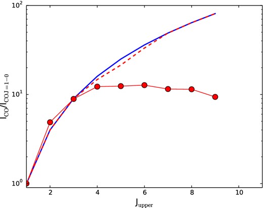
As an anecdotal example, consider the case of high-z submillimetre galaxies (SMGs). These 850-μm-selected galaxies typically live from z = 2 to 4, have star formation rates (SFRs) well in excess of 500 M⊙ yr−1 and are among the most luminous galaxies in the Universe (see the reviews by Blain et al. 2002; Casey, Narayanan & Cooray 2014). Originally, it was assumed that the gas was likely thermalized in these systems, given their extreme star formation rates (and likely extreme ISM densities and temperatures; e.g. Greve et al. 2005; Coppin et al. 2008; Tacconi et al. 2008). However, subsequent CO J = 1-0 observations of a small sample of SMGs with higher J detections by Hainline et al. (2006) and Harris et al. (2010) showed that a number of SMGs exhibit subthermal level populations, even at the modest excitation level of J = 3. Since then, it has become increasingly clear that SMGs are a diverse population (e.g. Hayward et al. 2011, 2012, 2013a,b; Bothwell et al. 2013; Hodge et al. 2013; Karim et al. 2013), with a large range in potential CO excitation ladders. To quantify this, in Fig. 1, we have compiled all of the CO SLEDs published to date for all high-z SMGs with a CO J = 1-0 detection. The diversity in the observed SLEDs is striking, even for one of the most extreme star-forming galaxy populations known. It is clear that no ‘template’ SLED exists for a given population.
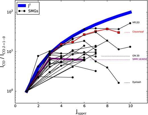
CO SLEDs for all known high-z SMGs with a CO J = 1-0 detection. A significant diversity in CO excitations exists, even for a given class of high-z galaxies, and it is evident that no universal line ratios are applicable. For a given line, roughly an order-of-magnitude uncertainty exists in the conversion ratio from high-J lines to the ground state. The blue line denotes J2, the scaling of intensities expected if the lines are all in the Rayleigh–Jeans limit and in local thermodynamic equilibrium (LTE). The red and purple lines denote the Cloverleaf quasar and SMG SMM 163650 – two galaxies that have similar SFRs, but starkly different SLEDs.
Nor can one do much better simply by comparing an observed galaxy to another galaxy with a known SLED and a similar luminosity or SFR. For example, turning again to Fig. 1, we highlight the SLED of a single quasar host galaxy denoted by the red line (the Cloverleaf quasar), and compare it to SMG SMM 163650 (purple). Both galaxies have estimated SFRs of roughly ∼1000 M⊙ yr−1 (Solomon et al. 2003; Weiß et al. 2003; Ivison et al. 2011), but they have dramatically different SLEDs. For the J = 6-5 line, there is roughly a factor of 5 difference in the SLEDs, and the discrepancy likely grows at even higher levels. It is clear from this example that extrapolating from high J lines to J = 1-0 using templates based on galaxies with similar global SFRs is a problematic approach.
The consequences of uncertainty in the excitation of CO are widespread in the astrophysics of star formation and galaxy formation. For example, observed estimates of the Kennicutt–Schmidt star formation relation at high redshift, an often-used observational test bed for theories of star formation in environments of extreme pressure (e.g. Ostriker & Shetty 2011; Krumholz, Dekel & McKee 2012; Faucher-Giguère, Quataert & Hopkins 2013), are dependent on assumed CO line ratios. Similarly, baryonic gas fractions of galaxies at high z, an observable diagnostic of the equilibrium established by gaseous inflows from the intergalactic medium (IGM), gas consumption by star formation and gas removal by winds, depend critically on observations of high-J CO lines, and their conversion to the J = 1-0 line (e.g. Tacconi et al. 2010; Bothwell et al. 2012; Davé, Finlator & Oppenheimer 2012; Krumholz & Dekel 2012; Narayanan, Bothwell & Davé 2012b; Forbes et al. 2013; Hopkins et al. 2013a,c; Saintonge et al. 2013). In the near future, CO deep fields will measure the CO luminosity function over a wide range of redshifts, and our ability to convert the observed emission into an estimate of |$\Omega _{\rm H_2}$|, the cosmic baryon budget tied up in H2 molecules, will depend on our understanding of the systematic evolution of CO SLEDs.
While some theoretical work has been devoted to modelling CO SLEDs from galaxies (Narayanan et al. 2008a; Narayanan, Cox & Hernquist 2008b; Narayanan et al. 2009; Armour & Ballantyne 2012; Lagos et al. 2012; Muñoz & Furlanetto 2013a,b; Popping et al. 2013a; Popping, Somerville & Trager 2013b), these models have by and large focused on utilizing synthetic CO excitation patterns to validate their underlying galaxy formation model. We lack a first-principles physical model for the origin of the shape of SLEDs in galaxies, and the relationship of this shape with observables. The goal of this paper is to provide one. The principal idea is that CO excitation is dependent on the gas temperatures, densities and optical depths in the molecular interstellar medium (ISM). Utilizing a detailed physical model for the thermal and physical structure of the star-forming ISM in both isolated disc galaxies and starbursting galaxy mergers, we investigate what sets these quantities in varying physical environments. We use this information to provide a parametrization of CO SLEDs in terms of the star formation rate surface density (ΣSFR), and show that this model compares very favourably with observed SLEDs for galaxies across a range of physical conditions and redshifts.
This paper is organized as follows. In Section 2, we describe our numerical modelling techniques, including details regarding our hydrodynamic models, radiative transfer techniques and ISM specification. In Section 3, we present our main results, including the principal drivers of SLED shapes, as well as a parametrized model for observed SLEDs in terms of the galaxy ΣSFR. In Section 4, we provide discussion, and we conclude in Section 5.
2 NUMERICAL MODELLING
2.1 Overview of models
The basic strategy that we employ is as follows, and is nearly identical to that employed by Narayanan et al. (2011b, 2012a). We first simulate the evolution of idealized disc galaxies and galaxy mergers over a range of masses, merger orbits and halo virial properties utilizing the smoothed particle hydrodynamics (SPH) code, gadget-3 (Springel & Hernquist 2003; Springel 2005; Springel, Di Matteo & Hernquist 2005). The goal of the idealized simulations is not to provide a simulated analogue of any particular observed galaxy, but rather to simulate a large range of physical conditions. As we will show, our simulations encapsulate a large range of molecular cloud densities, temperatures, velocity dispersions and CO optical depths.
We project the physical conditions of the SPH particles on to an adaptive mesh, and calculate the physical and chemical properties of the molecular ISM in post-processing. In particular, we determine the temperatures, mean cloud densities, velocity dispersions, H2–H i balance and fraction of carbon locked in CO. Determining the thermodynamic structure of the ISM involves balancing heating by cosmic rays and the grain photoelectric effect, energy exchange with dust, and CO and C ii line cooling. To calculate the line cooling rates, we employ the public code to Derive the Energetics and SPectra of Optically Thick Interstellar Clouds (despotic; Krumholz 2013), built on the escape probability formalism. The radiative transfer calculations determine the level populations via a balance of radiative absorptions, stimulated emission, spontaneous emission, and collisions with H2 and He. With these level populations in hand, we determine full CO rotational ladder for each cloud within our model galaxies. The observed SLED from the galaxy is just the combination of the CO line intensities at each level from each cloud in a given system.
At this point, the general reader should have enough background to continue to the results (Section 3) if they so wish. For those interested in the technical aspects of the simulation methodology, we elaborate further in the remainder of this section.
2.2 Hydrodynamic simulations of galaxies in evolution
The main purpose of the SPH simulations of galaxies in evolution is to generate a large number of realizations of galaxy models with a diverse range of physical properties. To this end, we simulate the hydrodynamic evolution of both idealized discs and mergers between these discs. Here, we summarize the features of the simulations most pertinent to this paper, and we refer the reader to Springel & Hernquist (2002, 2003) and Springel et al. (2005) for a more detailed description of the underlying algorithms for the hydrodynamic code employed, gadget-3.
The galaxies are exponential discs, and are initialized following the Mo, Mao & White (1998) formalism. They reside in live dark haloes, initialized with a Hernquist (1990) profile. We simulate galaxies that have halo concentrations and virial radii scaled for z = 0 and 3, following the relations of Bullock et al. (2001) and Robertson et al. (2006). The latter redshift choice is motivated by the desire to include a few extreme starburst galaxies in our simulation sample. The gravitational softening length for baryons is 100 h−1 pc, and 200 h−1 pc for dark matter.
The gas is initialized as primordial, with all metals forming as the simulation evolves. The ISM is modelled as multi-phase, with clouds embedded in a pressure-confining hotter phase (e.g. McKee & Ostriker 1977). In practice, this is implemented in the simulations via hybrid SPH particles. Cold clouds grow via radiative cooling of the hotter phase, while supernovae can heat the cold gas. Stars form in these clouds following a volumetric Schmidt (1959) relation, with index 1.5 (Kennicutt 1998a; Cox et al. 2006; Narayanan et al. 2011a; Krumholz et al. 2012). We note that in Narayanan et al. (2011b), we explored the effects of varying the Kennicutt–Schmidt star formation law index, and found that the ISM thermodynamic properties were largely unchanged so long as the index is ≥1. In either case, observations (e.g. Bigiel et al. 2008), as well as theoretical work (e.g. Krumholz, McKee & Tumlinson 2009b; Ostriker & Shetty 2011), suggest that the index may be superlinear in high-surface-density starburst environments.
The pressurization of the ISM via supernovae is implemented via an effective equation of state (EOS; Springel et al. 2005). In the models scaled for present epoch, we assume a modest pressurization (qEOS = 0.25), while for the high-z galaxies, we assume a more extreme pressurization (qEOS = 1). Tests by Narayanan et al. (2011b) show that the extracted thermodynamic properties of the simulations are relatively insensitive to the choice of EOS. Still, we are intentional with these choices. The high-z galaxies would suffer from runaway gravitational fragmentation, preventing starbursts, without sufficient pressurization. Because the simulations are not cosmological, and do not include a hot halo (e.g. Moster et al. 2011, 2012) or resolved feedback (Krumholz & Dekel 2010; Krumholz & Thompson 2012, 2013; Hopkins et al. 2013a,b), the early phases of evolution would quickly extinguish the available gas supply without sufficient pressurization. Despite this pressurization, large-scale kpc-sized clumps do still form from dynamical instabilities in high-z systems, similar to observations (Elmegreen, Klessen & Wilson 2008; Elmegreen et al. 2009a,b) and simulations (e.g. Dekel et al. 2009; Ceverino, Dekel & Bournaud 2010).
For the galaxy mergers, we simulate a range of arbitrarily chosen orbits. In Table 1, we outline the basic physical properties of the galaxies simulated here.
Galaxy evolution simulation parameters. Column 1 refers to the model name. Galaxies with the word ‘iso’ in them are isolated discs, and the rest of the models are 1:1 major mergers. Column 2 shows the baryonic mass in M⊙. Columns 3–6 refer to the orbit of a merger (with ‘N/A’ again referring to isolated discs). Column 7 denote the initial baryonic gas fraction of the galaxy and column 8 refers to the redshift of the simulation.
| Model | Mbar | θ1 | ϕ1 | θ2 | ϕ2 | fg | z |
|---|---|---|---|---|---|---|---|
| (M⊙) | |||||||
| 1 | 2 | 3 | 4 | 5 | 6 | 7 | 8 |
| z3isob6 | 3.8 × 10¹¹ | N/A | N/A | N/A | N/A | 0.8 | 3 |
| z3isob5 | 1.0 × 10¹¹ | N/A | N/A | N/A | N/A | 0.8 | 3 |
| z3isob4 | 3.5 × 10¹⁰ | N/A | N/A | N/A | N/A | 0.8 | 3 |
| z3b5e | 2.0 × 10¹¹ | 30 | 60 | −30 | 45 | 0.8 | 3 |
| z3b5i | 2.0 × 10¹¹ | 0 | 0 | 71 | 30 | 0.8 | 3 |
| z3b5j | 2.0 × 10¹¹ | −109 | 90 | 71 | 90 | 0.8 | 3 |
| z3b5l | 2.0 × 10¹¹ | −109 | 30 | 180 | 0 | 0.8 | 3 |
| z0isod5 | 4.5 × 10¹¹ | N/A | N/A | N/A | N/A | 0.4 | 0 |
| z0isod4 | 1.6 × 10¹¹ | N/A | N/A | N/A | N/A | 0.4 | 0 |
| z0isod3 | 5.6 × 10¹⁰ | N/A | N/A | N/A | N/A | 0.4 | 0 |
| z0d4e | 3.1 × 10¹¹ | 30 | 60 | −30 | 45 | 0.4 | 0 |
| z0d4h | 3.1 × 10¹¹ | 0 | 0 | 0 | 0 | 0.4 | 0 |
| z0d4i | 3.1 × 10¹¹ | 0 | 0 | 71 | 30 | 0.4 | 0 |
| z0d4j | 3.1 × 10¹¹ | −109 | 90 | 71 | 90 | 0.4 | 0 |
| z0d4k | 3.1 × 10¹¹ | −109 | 30 | 71 | −30 | 0.4 | 0 |
| z0d4l | 3.1 × 10¹¹ | −109 | 30 | 180 | 0 | 0.4 | 0 |
| z0d4n | 3.1 × 10¹¹ | −109 | −30 | 71 | 30 | 0.4 | 0 |
| z0d4o | 3.1 × 10¹¹ | −109 | 30 | 71 | −30 | 0.4 | 0 |
| z0d4p | 3.1 × 10¹¹ | −109 | 30 | 180 | 0 | 0.4 | 0 |
2.3 The physical and chemical properties of the molecular ISM
We determine the physical and chemical properties of the molecular ISM in post-processing. We project the physical properties of the SPH particles on to an adaptive mesh, utilizing an octree memory structure. Practically, this is done through the dust radiative transfer code sunrise (Jonsson 2006; Jonsson et al. 2006; Jonsson & Primack 2010; Jonsson, Groves & Cox 2010). The base mesh is 53 cells, spanning a 200 kpc box. The cells recursively refine into octs based on the refinement criteria that the relative density variations of metals (|$\sigma _{\rho _m}/\langle \rho _m \rangle$|) should be less than 0.1. The smallest cell size in the refined mesh is ∼70 pc across, reflecting the minimum cell size necessary for a converged dust temperature (Narayanan et al. 2010a).
We assume that all of the neutral gas in each cell is locked into spherical, isothermal clouds of constant density. The surface density is calculated directly from the gas mass and cell size. For cells that are very large, we consider the cloud unresolved, and adopt a subresolution surface density of Σcloud = 85 M⊙ pc−2, comparable to observed values of local GMCs (e.g. Solomon et al. 1987; Bolatto et al. 2008; Dobbs et al. 2013). The bulk of the H2 gas mass in our model galaxies, though, comes from resolved GMCs as the large cells in the adaptive mesh (that force the imposition of the threshold cloud surface density) correspond to low-density regions.
2.4 Thermodynamics and radiative transfer
A key part to calculating the observed SLED is the determination of the gas temperature in the model GMCs. The model is rooted in algorithms presented by Goldsmith (2001) and Krumholz, Leroy & McKee (2011), and tested extensively in models presented by Narayanan et al. (2011b, 2012a). Muñoz & Furlanetto (2013a,b) also use a similar approach. All our calculations here make use of the despotic package (Krumholz 2013), and our choices of physical parameters match the defaults in despotic unless stated otherwise.
despotic simultaneously solves equations (13)–(16) with equations (4) and (5) using an iteration process. We refer readers to Krumholz (2013) for details. We perform this procedure for every GMC in every model snapshot of every galaxy evolution simulation in Table 1. The result is a self-consistent set of gas and dust temperatures, and CO line luminosities, for every simulation snapshot. These form the basis for our analysis in the following section.
3 RESULTS
The CO SLED from galaxies represents the excitation of CO, typically normalized to the ground state. As the CO rotational levels are increasingly populated, the intensity (cf. equation 12) increases, and the SLED rises. When the levels approach local thermodynamic equilibrium (LTE), the excitation at those levels saturates. This is visible in the observational data shown in Fig. 1, where we showed the SLEDs for all SMGs with CO J = 1-0 detections. The Eyelash galaxy has modest excitation, with the SLED turning over at relatively low-J levels. By comparison, HFLS3, an extreme starburst at z ∼ 6 (Riechers et al. 2013), has levels saturated at J ∼ 7, with only a weak turnover at higher lying lines.
Our simulated galaxies reproduce, at least qualitatively, this range of behaviours. We illustrate this in Fig. 2, which shows our theoretically computed SLEDs for a sample of snapshots from model galaxy merger z0d4e. Each snapshot plotted has a different CO mass-weighted mean gas density and temperature. With increasingly extreme physical conditions, the populations in higher J levels rise, and the SLED rises accordingly. Eventually, the intensity from a given level saturates as it approaches thermalization.
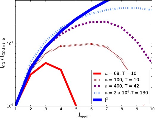
Model CO SLEDs for snapshots in a model galaxy merger with differing gas temperatures and densities. The blue line shows J2 scaling, the expected scaling of intensities for levels in LTE and in the Rayleigh–Jeans limit. As densities and temperatures rise, so does the SLED. It is important to note that an individual large velocity gradient or escape probability solution with the quoted temperatures and densities may not give the same simulated SLED as shown here for our model galaxies. Our model galaxy SLEDs result from the superposition of numerous clouds of varying density and temperature.
In this section, we more thoroughly explore the behaviour of the SLEDs in our simulations. First, in Section 3.1, we strive to understand the physical basis of variations in the SLEDs. Then, in Section 3.2, we use this physical understanding to motivate a parametrization for the SLED in terms of an observable quantity, the star formation surface density. We show that this parametrization provides a good fit to observed SLEDs in Section 3.3.
3.1 The drivers of SLED shapes in galaxies
The principal physical drivers of CO excitation are from collisions with H2and absorption of resonant photons. Generally, non-local excitation by line radiation is relatively limited on galaxy-wide scales (Narayanan et al. 2008c), and so the populations of the CO levels are set by a competition between collisional excitation and collisional and radiative de-excitation. Thus, the level populations in a given cloud are driven primarily by the density and temperature in that cloud, which affect collisional excitation and de-excitation rates, and by the cloud column density, which determines the fraction of emitted photons that escape, and thus the effective rate of radiative de-excitation. In this section, we examine these factors in three steps, first considering the gas temperature and density distributions, then the optical depth distributions, and finally the implications of the temperature on the shape of the SLED for thermalized populations.
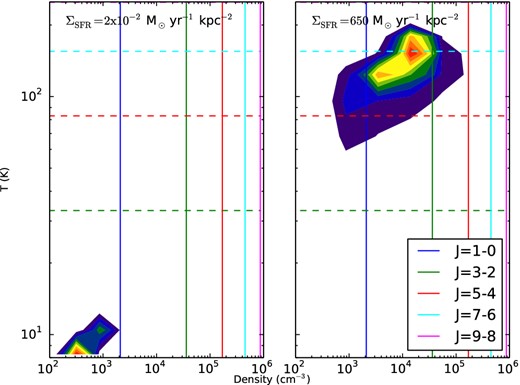
Distribution of GMCs in density–temperature phase space for two example simulated galaxies, one with low ΣSFR (left-hand panel) and one with high ΣSFR (right-hand panel). The main result from this figure is that gas in starburst environments is significantly warmer and denser than in quiescent environments. The left-hand panel shows a galaxy with ΣSFR ≈ 2 × 10⁻² M⊙ yr−1 kpc−2 (i.e. comparable to nearby quiescent disc galaxies), while the right shows a starburst with ΣSFR ≈ 650 M⊙ yr−1 kpc−2 (i.e. comparable to the nuclear regions of local ULIRGs and high-z SMGs). The innermost contour shows the region in the n-T plane where the H2 mass density exceeds 5.5 × 10⁷(1 × 10⁹) M⊙ dex−2 in the left (right) panel, and subsequent contours are spaced evenly in increments of 5.5 × 10⁶(1 × 10⁸) M⊙ dex−2. The horizontal dashed lines show Eupper/k for transitions CO J = 1-0 through 9-8 (alternating), and the vertical solid lines show the critical density, ncrit, for the same transitions at an assumed temperature of T = 100 K, and are taken from the Carilli & Walter (2013) review. We note that critical densities depend on temperature (via collisional rates), though only weakly.
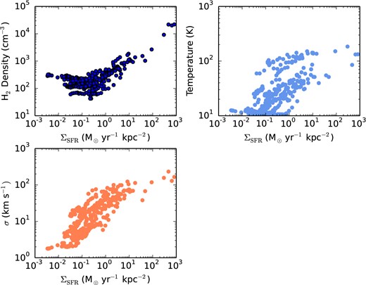
CO mass-weighted H2 gas densities, kinetic temperatures and velocity dispersions of GMCs in each of our model galaxy snapshots as a function of galaxy ΣSFR. Each point represents a single snapshot from a single simulation. Note that, at high ΣSFR, the physical conditions become increasingly extreme in our model galaxies.
3.1.1 Gas density and temperature
By and large, molecular clouds in normal, star-forming disc galaxies at z ∼ 0 (like the Milky Way) have relatively modest mean gas densities, with typical values n ≈ 10-500 cm−3. This is evident from both Figs 3 and 4. Three major processes can drive deviations from these modest values, and greatly enhance the mean gas density of molecular clouds. First, very gas rich systems will be unstable, and large clumps of gas will collapse to sustain relatively high SFRs. These galaxies are represented by early-phase snapshots of both our model discs and model mergers, and serve to represent the modest increase in galaxy gas fraction seen in high-z star-forming galaxies (Narayanan et al. 2012b; Haas et al. 2013; Ivison et al. 2013). Secondly, galaxy mergers drive strong tidal torques that result in dense concentrations of nuclear gas, again associated with enhanced SFRs (Mihos & Hernquist 1994a,b; Younger et al. 2009; Hayward et al. 2013c; Hopkins et al. 2013a,c). The mass-weighted mean galaxy-wide H2 gas density in the most extreme of these systems can exceed 103 cm−3, with large numbers of clouds exceeding 104 cm−3 (cf. fig. A2 of Narayanan et al. 2011b). This is highlighted by the right-hand panel of Fig. 3, which shows the distribution of molecular gas in the n-T plane for such a nuclear starburst. Finally, large velocity dispersions in GMCs can enhance the mean density via a turbulent compression of gas (cf. equation 2.) In all three cases, the increased gas densities are correlated with enhanced galaxy-wide SFR surface densities, in part owing to the enforcement of a Kennicutt–Schmidt star formation law in the SPH simulations.4
Increased gas kinetic temperatures can also drive up the rate of collisions between CO and H2, thereby increasing molecular excitation. As discussed by Krumholz et al. (2011) and Narayanan et al. (2011b), the gas temperature in relatively quiescent star-forming GMCs is roughly ∼10 K. In our model, this principally owes to heating by cosmic rays. At the relatively low densities (10–100 cm−3) of normal GMCs, heating by energy exchange with dust is a relatively modest effect, and cosmic rays tend to dominate the gas heating. For a cosmic ray ionization rate comparable to the Milky Way's, a typical GMC temperature of ∼10 K results (Narayanan & Hopkins 2013).5
As galaxy SFRs increase, however, so do the gas temperatures. This happens via two dominant channels. In our models, the cosmic ray ionization rate scales linearly with the galaxy-wide SFR, motivated by tentative trends observed by Acciari et al. (2009), Abdo et al. (2010) and Hailey-Dunsheath et al. (2008a). As noted by Papadopoulos (2010), Papadopoulos et al. (2011) and Narayanan & Davé (2012a,b), increased cosmic ray heating rates can substantially drive up gas kinetic temperatures, depending on the density of the gas and cosmic ray flux. Secondly, at gas densities above ∼104 cm−3, the energy exchange between gas and dust becomes efficient enough that collisions between H2 and dust can drive up the gas temperature as well. Because high SFRs accompany high gas densities, and high dust temperatures typically accompany high SFRs (e.g. Narayanan et al. 2010b), the gas temperature rises with the galaxy SFR. At very large densities (n ≫ 104 cm−3), we find that the dust temperatures are typically warm enough that the heating by cosmic rays is a minor addition to the energy imparted to the gas by collisions with dust. As is evident from Fig. 4, because both heating channels scale with the observable proxy of SFR surface density, the mean galaxy-wide gas temperature does as well. For galaxies undergoing intense star formation, the mean gas temperature across the galaxy can approach ∼100 K.
3.1.2 Line optical depths
In Fig. 5, we show the median CO luminosity-weighted optical depth for a sample of CO transitions as a function of galaxy SFR surface density. The lines in Fig. 5 can be thought of as the typical optical depth for different CO lines within the GMCs in our model galaxies. In short, low-J CO transitions are always optically thick, while high-J lines only become optically thick in more extreme star-forming galaxies. Referring to equation (16), the qualitative trends are straightforward to interpret, and arise from a combination of both the varying level populations and changing physical conditions as a function of galaxy ΣSFR. Low-lying transitions such as CO J = 1-0 are typically thermalized in most clouds in galaxies (even at low ΣSFR), owing to the relatively low critical densities and high optical depths. Hence, in even more dense conditions in high-ΣSFR systems, the relative level populations stay approximately constant. However, the optical depth is inversely proportional to the gas velocity dispersion which tends to rise with SFR surface density (cf. Fig. 4). Hence, at increased ΣSFR, the optical depths of low-J transitions decrease slightly, though they remain optically thick. The opposite trend is true for high-J transitions. These transitions are typically subthermally populated in low-density clouds. As densities and temperatures rise with ΣSFR, so do the level populations. This rise offsets the increase in gas velocity dispersion, and the optical depths in these lines increase in more extreme star-forming systems.
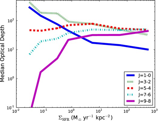
CO line luminosity-weighted line optical depths as a function of galaxy ΣSFR. Each line represents the median luminosity-weighted line optical depth for all snapshots within bins of ΣSFR. The low-J CO lines start off roughly thermalized. At increased ΣSFR, the gas velocity dispersions increase, and photons in these lines are more easily able to escape, decreasing the optical depths. For high-J transitions, the level populations begin at modest levels, and the optical depths are low. Broadly, at increased ΣSFR, the level populations rise owing to increased gas densities and temperatures, which drives the optical depths up.
The net effect of the mean trends in CO optical depths in molecular clouds in star-forming galaxies, as summarized in Fig. 5, is that galaxies of increased gas density and temperature (as parametrized here by increased ΣSFR) have increased optical depths in high-J CO lines. This drives down the effective density, and lets the levels achieve LTE more easily. This will be important for explaining how some observed high-J CO lines (such as J = 7-6) can exhibit line ratios comparable to what is expected from LTE, despite the fact that galaxy-wide mean densities rarely reach ∼105 cm−3, the typical critical density for high-J CO emission (cf. Fig. 3).
3.1.3 Line ratios for thermalized populations
Thus far, we have been principally concerned with the physical drivers of CO excitation, as well as the influence of optical depth in lowering the effective density for thermalization of a given CO line. These have given some insight as to roughly when SLED lines will saturate. We now turn our attention to what values line ratios will have when they approach thermalization. The intensity of a line for level populations that are in LTE is given by the Planck function at that frequency. In the Rayleigh–Jeans limit, when Eupper ≪ kT, the observed line ratios (compared to the ground state) scale as J2.
In Fig. 6, we plot the CO line luminosity-weighted gas kinetic temperature as a function of galaxy SFR surface density for a selection of CO transitions. To guide the eye, we also plot as horizontal (dashed) lines the values of Tupper = Eupper/k for the same transitions. At even low values of ΣSFR, the CO J = 1-0 and 3-2 emitting gas temperature is a factor of ∼ 5-10 larger than Eupper/k. The gas that emits higher lying lines (e.g. J = 5-4) has temperatures roughly twice Eupper/k for the most extreme systems, while higher lying lines do not approach the Rayleigh–Jeans limit even for the most extreme galaxies. As a consequence, for high-ΣSFR galaxies, we can expect line ratios (compared to the ground state) to scale as J2 for lower lying lines. For higher J lines in LTE (Jupper ≳ 7), the line ratios will simply follow the ratio of the Planck functions for the levels, giving rise to a SLED that is flatter than J2.
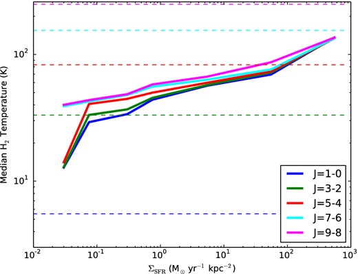
CO line luminosity-weighted median gas kinetic temperatures as a function of galaxy ΣSFR. The horizontal dashed lines show the temperature Tupper = Eupper/k that corresponds to the upper level energy of a given CO transition (with the same colour coding as the solid lines). At even modest ΣSFR, gas temperatures as such that lines through CO J = 4-3 are well into the Rayleigh–Jeans limit. In contrast, even at the most extreme ΣSFR values in our library, the median gas temperature is never high enough to exceed Tupper for Jupper ≥ 7.
3.2 A parametrized model for CO SLEDs
Owing to both a desire for high resolution and sensitivity, as well as the general prevalence of (sub)mm-wave detectors that operate between 800 μm and ∼3 mm, observations of high-z galaxies are often of rest-frame high-J CO lines. Because physical measurements of H2 gas masses require conversion from the CO J = 1-0 line, we are motivated to utilize our model results to derive a parametrized model of the CO excitation in star-forming galaxies.
From Fig. 2, it is clear that the SLED from galaxies rises with increasing H2 gas density and kinetic temperature. How rapidly these SLEDs rise depends on the exact shape of the density and temperature probability distribution function (PDF), as well as the line optical depths. As we showed in Section 3.1.3, the SLED tends to saturate at roughly J2 for Jupper ≲ 6 at high ΣSFR, owing to large gas kinetic temperatures (cf. Fig. 6). For higher lying lines, when the levels are in LTE, the SLED will saturate at the ratio of the Planck functions between Jupper and the ground state.
In principle, the SLED would best be parametrized by a combination of the gas densities, temperatures and optical depths. Of course, these quantities are typically derived from observed SLEDs, not directly observed. However, as shown in Figs 3–5, these quantities are reasonably well correlated with the SFR surface density of galaxies. Qualitatively, this makes sense – more compact star-forming regions arise from denser gas concentrations. Similarly, regions of dense gas and high SFR density have large UV radiation fields (and thus warmer dust temperatures), increased efficiency for thermal coupling between gas and dust, and increased cosmic ray heating rates.
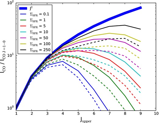
parametrized model for SLEDs. The model SLED shape is a function of ΣSFR, and is given in equation (19), with fit parameters listed in Tables 2 and 3. The solid lines show the perfectly resolved case, while the dashed lines (of the same colour) show the case for unresolved models. Unresolved observations share the same assumed emitting area, and therefore depress the SLEDs at high J because the emitting gas occupies a smaller area, and therefore suffers beam dilution when averaged over the same area as the low-J lines.
Fits to equation (19) for resolved observations of galaxies.
| Line ratio | A | B | C |
|---|---|---|---|
| (|$I_{ij}/I_{\rm 1{\rm -}0}$|) | |||
| CO J = 2-1 | 0.09 | 0.49 | 0.47 |
| CO J = 3-2 | 0.17 | 0.45 | 0.66 |
| CO J = 4-3 | 0.32 | 0.43 | 0.60 |
| CO J = 5-4 | 0.75 | 0.39 | 0.006 |
| CO J = 6-5 | 1.46 | 0.37 | −1.02 |
| CO J = 7-6 | 2.04 | 0.38 | −2.00 |
| CO J = 8-7 | 2.63 | 0.40 | −3.12 |
| CO J = 9-8 | 3.10 | 0.42 | −4.22 |
In principle, the numbers presented in Table 2 allow for the calculation of the full SLED of a galaxy given a measured ΣSFR. This said, an essential point to the SLED calculations presented thus far is that CO intensities for a given line are resolved at the level of our finest cell in our adaptive mesh (∼70 pc). Thus, Table 2 provides reliable parameters for a SLED construction from the SFR surface density given that the emitting region in each line is resolved. In other words, if a given high-J line is observed from a galaxy (say, CO J = 4-3), to convert down to the J = 1-0 transition utilizing equation (19) and the fit parameters in Table 2, the CO J = 4-3 region must have been resolved. For observations of local galaxies with interferometers [e.g. Atacama Large Millimetre Array (ALMA)], this is plausible, and even likely. For high-redshift observations, or observations of local galaxies using coarse beams, however, it is likely that the observations will be unresolved.
In the case of unresolved observations, the emitting area utilized in intensity calculations is typically a common one across transitions, and therefore misses the clumping of the principal emitting regions of higher lying CO transitions. In this case, Table 2 will not provide an appropriate description of the observed SLED. To account for this, we determine the luminosity-weighted emitting area for each transition of each model galaxy snapshot, and scale the intensity of the line accordingly. We then re-fit the line ratios as a function of ΣSFR, and present the best-fitting parameters for unresolved observations in Table 3. The effect of an unresolved observation is clear from Fig. 7, where we show the unresolved counterparts to the resolved SLEDs with the dashed curves. For a given transition, the solid line shows the resolved SLED from our model parametrization, and the dashed the unresolved excitation ladder. Because high-J lines tend to arise from warm, dense regions that are highly clumped compared to the CO J = 1-0 emitting area, the resultant SLED is decreased compared to highly resolved observations. This effect was previously noted for models high-z SMG models by Narayanan et al. (2009).
Fits to equation (19) for unresolved observations of galaxies.
| Line ratio | A | B | C |
|---|---|---|---|
| (|$I_{ij}/I_{\rm 1{\rm -}0}$|) | |||
| CO J = 2-1 | 0.07 | 0.51 | 0.47 |
| CO J = 3-2 | 0.14 | 0.47 | 0.64 |
| CO J = 4-3 | 0.27 | 0.45 | 0.57 |
| CO J = 5-4 | 0.68 | 0.41 | −0.05 |
| CO J = 6-5 | 1.36 | 0.38 | −1.11 |
| CO J = 7-6 | 1.96 | 0.39 | −2.14 |
| CO J = 8-7 | 2.57 | 0.41 | −3.35 |
| CO J = 9-8 | 2.36 | 0.50 | −3.70 |
In conjunction with this paper, we provide idl and python modules for reading in the parametrized fits from Tables 2 and 3, and host these at a dedicated web page, as well as at https://sites.google.com/a/ucsc.edu/krumholz/codes.
3.3 Comparison to observations
In an effort to validate the parametrized model presented here, in Fig. 8 we present a comparison between our model for CO excitation in galaxies and observations of 15 galaxies from present epoch to z > 6. Most of the observational data come from galaxies at moderate to high redshift owing to the fact that it is typically easier to access the high-J submillimetre CO lines when they are redshifted to more favourable atmospheric transmission windows than it is at z ∼ 0. With the exception of NGC 253, we use our fits for unresolved observations in this comparison. For NGC 253, we use the resolved model, because that galaxy is only ≈3.3 Mpc away (Rekola et al. 2005), and the CO observations were made with fairly high resolution, so that the high-J emitting regions were likely resolved. The blue solid lines in each panel show the J2 scaling of intensities expected for thermalized levels in the Rayleigh–Jeans limit.
![Compilation of 15 observed CO SLEDs (solid coloured points) for galaxies at low and high z. The panels are sorted in order of decreasing ΣSFR, and span a dynamic range of roughly 200. Each panel is labelled by the value of ΣSFR, in units of M⊙ kpc−2 yr−1, and the redshift of the galaxy. The dashed line in each panel shows the model prediction derived in this paper [equation (19) and Table 3 for all galaxies but NGC 253, equation (19) and Table 2 for NGC 253, which is spatially resolved]. The solid blue lines show I ∝ J2, the scaling expected for thermalized populations in the Rayleigh–Jeans limit. The data shown are from the following sources: Riechers et al. (2011, 2013), Barvainis et al. (1994, 1997), Wilner, Zhao & Ho (1995), Weiß et al. (2003), Alloin et al. (1997), Yun et al. (1997), Bradford et al. (2003, 2009), Fu et al. (2013), Danielson et al. (2011), Casey et al. (2009), Carilli et al. (2010), Daddi et al. (2009, 2010), Dannerbauer et al. (2009), Hodge et al. (2012), Kamenetzky et al. (2012), Ivison et al. (2011, 2013), Hailey-Dunsheath et al. (2008b), Meijerink et al. (2013), Papadopoulos et al. (2012) and van der Werf et al. (2010). The bulk of the ΣSFR values were either reported in the original CO paper or in Kennicutt (1998b). The exceptions are as follows. The values of ΣSFR for the Eyelash galaxy and GN20 were provided via private communication from Mark Swinbank and Jackie Hodge, respectively. For SMM 123549, 163650 and 163658, ΣSFR values were calculated by converting from LFIR to SFR utilizing the calibration in Murphy et al. (2011) and Kennicutt & Evans (2012), and the galaxy sizes reported in Ivison et al. (2011). The size scale for the Cloverleaf quasar was taken from the CO J = 1-0 measurements by Venturini & Solomon (2003) for the ΣSFR calculation, and SFR reported in Solomon et al. (2003). The ΣSFR value for Mrk 231 was calculated by via the SFR reported for the central disc by Carilli, Wrobel & Ulvestad (1998) and the size of the disc derived by Bryant & Scoville (1996).](https://oup.silverchair-cdn.com/oup/backfile/Content_public/Journal/mnras/442/2/10.1093/mnras/stu834/2/m_stu834fig8.jpeg?Expires=1749871581&Signature=4Byn4sC5f~16DbyMB0pslgo2imffURstWM22-JeVp2CnGCEXhtKFkOXAoQhT6yXfQvIjOK7hEpUDguiDM~WFjelb8B0oGiFTkb85ojXAaoNvEPGJNoNjINlsWqPJfpUc81fttoHwOpvKF9gqZVtvVjROVOE3GJTDD0vZ5QBONNWoVOBPacdO6O8cLb5BznTg~KKCuxU--ozKDWpsG7wYpQd4-Ku9AIbtEEEJ57ElC3fLUzsRsKcxAnvpQKF4~QIvLu2IQ69bu2OvD2QAklrqd1EyQ88r9A6H47gI5fYKwoov-ygQdtC777LMh2knbnzjXVuOkSnC4LGd1uiDQIFJWA__&Key-Pair-Id=APKAIE5G5CRDK6RD3PGA)
Compilation of 15 observed CO SLEDs (solid coloured points) for galaxies at low and high z. The panels are sorted in order of decreasing ΣSFR, and span a dynamic range of roughly 200. Each panel is labelled by the value of ΣSFR, in units of M⊙ kpc−2 yr−1, and the redshift of the galaxy. The dashed line in each panel shows the model prediction derived in this paper [equation (19) and Table 3 for all galaxies but NGC 253, equation (19) and Table 2 for NGC 253, which is spatially resolved]. The solid blue lines show I ∝ J2, the scaling expected for thermalized populations in the Rayleigh–Jeans limit. The data shown are from the following sources: Riechers et al. (2011, 2013), Barvainis et al. (1994, 1997), Wilner, Zhao & Ho (1995), Weiß et al. (2003), Alloin et al. (1997), Yun et al. (1997), Bradford et al. (2003, 2009), Fu et al. (2013), Danielson et al. (2011), Casey et al. (2009), Carilli et al. (2010), Daddi et al. (2009, 2010), Dannerbauer et al. (2009), Hodge et al. (2012), Kamenetzky et al. (2012), Ivison et al. (2011, 2013), Hailey-Dunsheath et al. (2008b), Meijerink et al. (2013), Papadopoulos et al. (2012) and van der Werf et al. (2010). The bulk of the ΣSFR values were either reported in the original CO paper or in Kennicutt (1998b). The exceptions are as follows. The values of ΣSFR for the Eyelash galaxy and GN20 were provided via private communication from Mark Swinbank and Jackie Hodge, respectively. For SMM 123549, 163650 and 163658, ΣSFR values were calculated by converting from LFIR to SFR utilizing the calibration in Murphy et al. (2011) and Kennicutt & Evans (2012), and the galaxy sizes reported in Ivison et al. (2011). The size scale for the Cloverleaf quasar was taken from the CO J = 1-0 measurements by Venturini & Solomon (2003) for the ΣSFR calculation, and SFR reported in Solomon et al. (2003). The ΣSFR value for Mrk 231 was calculated by via the SFR reported for the central disc by Carilli, Wrobel & Ulvestad (1998) and the size of the disc derived by Bryant & Scoville (1996).
Fig. 8 shows that the model performs quite well over a very large dynamic range in galaxy properties. Over all transitions in all galaxies in Fig. 8, the median discrepancy between observations and our model is 25 per cent, and the maximum ratio is a factor of ∼2. In comparison, for the observed set of SMGs presented in Fig. 1, the maximum difference in line ratios at a given transition is ∼30. The galaxies shown range from local starbursts to relatively normal star-forming galaxies at high-z to high-z SMGs to some of the most luminous, heavily star-forming galaxies discovered to date (e.g. GN20 and HFLS3). Their star formation surface densities vary by roughly a factor of 200. Our model captures both the qualitative and quantitative behaviour of the SLEDs over this full range.
While the SFR surface density provides a relatively good parametrization for the observed SLED from a star-forming galaxy, the global SFR does not. This is because the global SFR does not correlate well with the density and temperature PDFs in clouds. As an example, in Fig. 9 we plot the (resolved) simulated SLED for two galaxies with very similar global SFRs. One is a galaxy merger and the other a gas-rich disc galaxy comparable to conditions in high-z discs. The galaxy merger is more compact, and therefore has a significantly higher ΣSFR than the relatively distributed star formation characteristic of the gas-rich disc. As a result, though the global SFRs of the galaxies are similar, the physical conditions within the molecular clouds of the systems are not, and the resultant observed SLEDs diverge. Similar divergences can be found in observations. For example, compare the Cloverleaf quasar to the SMG SMM 163650 in Fig. 1. Both galaxies have incredible global SFRs of ∼1000 M⊙ yr−1 (Solomon et al. 2003; Weiß et al. 2003; Ivison et al. 2011), but they clearly have starkly different CO SLEDs.6
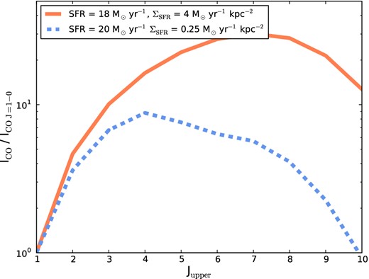
Simulated resolved CO SLEDs for two model galaxies with similar SFRs, but differing star formation rate surface densities (ΣSFR). While two galaxies may have the same global SFR, the physical conditions in the ISM may vary strongly leading to very different SLEDs. The star formation surface density ΣSFR provides a much better parametrization.
4 DISCUSSION
4.1 The parametrization of SLEDs
We have presented a model the physical origins of SLEDs in star-forming galaxies, and derived a rough parametrization of the SLED in terms of an observable quantity, the star formation rate surface density. As discussed in Section 3.2, as well as in Fig. 9, the global SFR alone provides a poor parametrization of the CO SLED and, more generally, the physical conditions in the molecular clouds in the galaxy.
A number of other works have arrived at similar conclusions, though via notably different methods. As an example, Rujopakarn et al. (2011) showed that galaxies with similar infrared luminosity densities across different redshifts shared more common observed properties (such as aromatic features) than simply galaxies at a shared infrared luminosity. This is akin to the idea that ULIRGs at z ∼ 0 do not lie on the SFR–M* main sequence, while galaxies of a comparable luminosity at high z do (Daddi et al. 2005; Rodighiero et al. 2011). In contrast, normalizing by the spatial scale of the emitting (or star-forming) region allows for a more straightforward comparison of galaxies even at vastly different redshifts. A similar point was made by Hopkins et al. (2010), who showed that with increasing redshift, the fraction of galaxies at a given luminosity comprised of galaxy mergers and starbursts decreases dramatically.
This point is related to that made by Díaz-Santos et al. (2013), when examining the [C ii]–FIR deficit in galaxies. At z ∼ 0, galaxies with large infrared luminosity tend to have depressed [C ii] 158 μm emission as compared to what would be expected for the typical [C ii]–FIR scaling at lower luminosities (Malhotra et al. 1997; Luhman et al. 1998; de Looze et al. 2011; Farrah et al. 2013). While the origin of the deficit is unknown, early indications suggest that a similar deficit may exist in high-z galaxies, though offset in infrared space (e.g. Stacey et al. 2010; Graciá-Carpio et al. 2011; Wang et al. 2013). However, Díaz-Santos et al. (2013) showed that when comparing to a galaxy's location with respect to the specific SFR main sequence, galaxies at both low and high z follow a similar trend.
As a result of this, there are no ‘typical’ values of CO SLEDs for a given galaxy population. Populations such as ULIRGs or SMGs are generally selected via a luminosity or colour cut. This can result in a heterogeneous set of physical conditions in galaxies, and therefore heterogeneous CO emission properties. This was shown explicitly by Papadopoulos et al. (2012), who demonstrated that local luminous infrared galaxies (LIRGs; LIR ≥ 1011 L⊙ ) exhibit a diverse range of CO excitation conditions. Similarly, Downes & Solomon (1998), Tacconi et al. (2008), Magdis et al. (2011), Hodge et al. (2012), Magnelli et al. (2012), Ivison et al. (2013) and Fu et al. (2013) showed that the CO–H2 conversion factor, XCO, for ULIRGs and that for high-z SMGs each show a factor of ∼5–10 range in observationally derived values. A template for the CO emission properties is not feasible for a given galaxy population given the wide variation in ISM physical conditions that can be found in luminosity-selected populations.
4.2 Relationship to other models
Over the last few years, a number of theoretical groups have devoted significant attention to predicting CO emission from star-forming galaxies. Here, we review some previous efforts to predict CO SLEDs, and place our current work into this context. In short, a number of analytic models and SAMs have explored the simulated SLEDs from model galaxies, but no comprehensive model for the origin of SLEDs has been reported thus far. Most works focus on validation of a given galaxy formation model.
To date, no work investigating SLEDs has utilized bona fide hydrodynamic simulations of galaxy evolution that directly simulate the physical properties of the ISM to calculate the CO excitation from galaxies. They have instead relied on either analytic models or SAMs to describe the physical properties of galaxies and GMCs within these galaxies, and coupled these analytic models with numerical radiative transfer calculations to derive the synthetic CO emission properties.
On the purely analytic side, Armour & Ballantyne (2012) and Muñoz & Furlanetto (2013b) developed models for quiescent disc galaxy evolution (constructing such a model for merger-driven starbursts would be quite difficult) in order to predict CO emission from nuclear starburst discs around active galactic nuclei (AGN), and from z ≳ 6 galaxies, respectively. Armour & Ballantyne (2012) construct single-phase nuclear discs that rotate around a central AGN. The SFR is forced to be such that Toomre's Q parameter is unity, and the vertical support of the disc owes to radiative feedback following the theory of Thompson, Quataert & Murray (2005). The CO SLEDs are calculated by applying ratran radiative transfer calculations to the model grid (Hogerheijde & van der Tak 2000). These authors find that nuclear starbursts are extremely dense, and therefore thermalized line ratios will be common. A subset of the models show strong correspondence with the M82, Mrk 231 and Arp 220, with potentially some underprediction of the highest J transitions (J > 8). Interestingly, a subset of the models by Armour & Ballantyne (2012) fall into CO line absorption at large Jupper (Jupper > 11), owing to the steep temperature and density gradients within the starburst.
Muñoz & Furlanetto (2013b) develop analytic models of high-z galaxy discs that also are forced to maintain vertical hydrostatic equilibrium by radiation pressure, similar to the aforementioned study by Armour & Ballantyne (2012). Muñoz & Furlanetto (2013b) place their galaxies in a cosmological context by allowing for gas accretion from the IGM following parametrizations from cosmological dark matter simulations, as well as allow for momentum-driven winds following the Oppenheimer & Davé (2008) prescriptions. Within the discs, GMCs are assumed to have a threshold floor surface density of 85 M⊙ pc−2, and H2 fractions that depend on the stellar and cloud surface density. The CO fraction follows the Wolfire et al. (2010) model, as in our work, and the GMCs have lognormal density distribution following from supersonic turbulence. After accounting for the modulation of critical densities by line optical depths, Muñoz & Furlanetto (2013b) calculate the CO excitation of their model z ∼ 6 galaxies utilizing a precursor code to despotic, with identical underlying algorithms. These authors focused specifically on the observable CO J = 6-5 line. They find that the high-J lines from these galaxies will be observable with ALMA, as long as the ISM clumps similarly to local galaxies. If turbulence does not provide the principal support for the clouds, however, and they are more homogeneous, the excitation of high-J levels will be greatly reduced. This said, Muñoz & Furlanetto (2013a) suggest that their model may overpredict the expected CO J = 6-5 emission from extreme star-formers at high z such as the z ∼ 6 SMG HFLS3, in part due to the high gas velocity dispersions (and thus an increased gas median density due to turbulent compression of gas; cf. equation 2). Indeed, their model has similar velocity dispersions for HFLS3-like systems as our own (∼100 km s−1). While it is difficult to exactly compare our model with that of Muñoz & Furlanetto (2013a) owing to the starkly different modelling methods (analytic versus coupled hydrodynamic and radiative transfer), one possible origin in the difference in predicted SLEDs for HFLS3-like systems is in the radial density distribution within the gas. In our model, a sufficiently large low-density emitting region exists even in high-ΣSFR galaxies that the unresolved model SLED is depressed at high-J levels.
Turning to SAMs, Lagos et al. (2012) coupled the galform SAM with the 1D PDR code ucl_pdr (Bayet et al. 2011) to analyse the model CO emission from analytic galaxies painted on to dark matter haloes taken from N-body simulations. These authors assume H2 fractions that derive from the empirical relations provided by Blitz & Rosolowsky (2006) for normal star-forming galaxies,7 and an H2 fraction of unity in starbursts. The PDR modelling assumes that the gas is confined to a one-zone slab geometry illuminated on one side by a UV field, which scales with ΣSFR in the Lagos et al. (2011, 2012) version of galform. For the majority of their models, Lagos et al. (2012) assume isodensity gas of nH = 104 cm−3, and calculate the SLEDs accordingly. They find that on average the SLEDs of galaxies that are LIRGs (ULIRGs) at z = 0 peak at J = 4(5), though there is significant dispersion in the high-J excitation. While difficult to directly compare with our own work, the range of SLEDs derived by Lagos et al. (2012) is certainly consistent with the range found here.
Following on this, Popping et al. (2013a,b) coupled a SAM for galaxy formation (Somerville et al. 2008a) with the radiative transfer code β3d (Poelman & Spaans 2005, 2006; Pérez-Beaupuits, Wada & Spaans 2011) to model the CO (among other species) emission from their model galaxies. The H2 fraction is based on fitting functions from cosmological zoom simulations by Gnedin & Kravtsov (2011), dependent on the stellar and gas surface densities. Star formation follows a modified Kennicutt–Schmidt star formation relation (Kennicutt 1998b; Kennicutt & Evans 2012), and clouds occupy a volume filling factor of fclump = 0.01. These authors find excellent agreement in the dense gas fractions returned by their models (as traced by observed dense gas line ratios – Narayanan et al. 2005; Bussmann et al. 2008; Juneau et al. 2009; Hopkins et al. 2013b) and observations. Relevant to the present study, Popping et al. (2013a) find that galaxies with higher far-infrared (FIR) luminosities have CO SLEDs that peak at higher excitation levels, similar to the work by Lagos et al. (2012). Galaxies at a fixed FIR luminosity in this model, though, peak at higher CO levels at high redshifts than at low redshifts. In the Popping et al. (2013a) model, this owes to the fact that galaxies at high z at a fixed FIR have warmer and denser cold gas than their low-z counterparts do. While we are unable to make a similar comparison, in our model this could be ascribed to galaxies at high z at a fixed luminosity having higher ΣSFR than their low-z analogues. This is likely the case in the Popping et al. (2013a) model, as the disc sizes of galaxies at a fixed stellar mass are smaller at high z than present epoch (Somerville et al. 2008b). Popping et al. (2013a) show a steeply rising relation between CO level populations and Σgas (which is presumably similar to the relation with ΣSFR given their star formation law), and a much more moderate relationship between molecular level populations and global galaxy SFR. In this sense, our work is seemingly in very good agreement with the Popping et al. (2013a) model.
4.3 Applications of this model
With the power-law fit presented in equation (19) and Tables 2 and 3, we have provided a mechanism for calculating the full CO rotational ladder through the J = 9-8 transition given a constraint on the SFR surface density. With this, in principle one can utilize a CO observation of a high-z galaxy at an arbitrary transition, and then down-convert to the CO J = 1-0 transition flux density.
To convert from the CO J = 1-0 flux density to the more physically meaningful H2 gas mass, one needs to employ a CO–H2 conversion factor. While there have been numerous observational (Magdis et al. 2011; Donovan Meyer et al. 2012; Genzel et al. 2012; Hodge et al. 2012; Schruba et al. 2012; Blanc et al. 2013; Bolatto, Wolfire & Leroy 2013; Fu et al. 2013; Sandstrom et al. 2013) and theoretical (Feldmann, Gnedin & Kravtsov 2011, 2012; Glover & Mac Low 2011; Narayanan et al. 2011b, 2012a; Shetty et al. 2011a,b; Lagos et al. 2012) attempts to constrain the CO–H2 conversion factor, significant uncertainty exists in the calibration.
The coupling of the model for CO SLEDs in this work, with the formalism for deriving H2 gas masses in equations (20) and 21, in principle could allow for the direct determination of an H2 gas mass of a high-z galaxy with measurements (or assumptions) of a CO surface brightness (at any J level up to J = 9-8), a ΣSFR and a gas phase metallicity. This may have implications for derived properties of high-z galaxies.
For example, galaxy baryonic gas fractions at high z are measured to be substantially larger than in the local Universe (e.g. Daddi et al. 2010; Tacconi et al. 2010; Geach et al. 2011; Popping et al. 2012; Sandstrom et al. 2013). Correctly measuring these and relating them to galaxy formation models in which the gas fraction is set by a combination of accretion from the IGM, star formation and gas outflows (e.g. Davé et al. 2012; Gabor & Bournaud 2013) will depend not only on the conversion from CO J = 1-0 to H2 gas masses (cf. Narayanan et al. 2012b), but also a correct down-conversion from the measured excited CO emission line to the ground state. Systematic trends in the excitation with galaxy physical property will, of course, muddy comparisons between observation and theory further.
Similarly, measurements of the Kennicutt–Schmidt star formation relation at high z are sensitively dependent on gas excitation in galaxies. In principle, if there is a strong relationship between gas excitation and galaxy physical conditions, one might expect that inferred star formation laws from high-excitation lines will be flatter than the true underlying relation. Krumholz & Thompson (2007) and Narayanan et al. (2008b,c) showed that the local SFR–LHCN and SFR–LCO relation can be strongly affected by increasing level populations of the HCN molecule. This work was furthered by Narayanan et al. (2011a) who used a more rudimentary model of the calculations presented here to find that inferred linear star formation laws at high z potentially suffered from differential excitation, and that the true underlying slope was steeper. As large surveys of galaxies at high z fill in the ΣSFR-Σgas relation, accurate conversions from highly excited lines to the J = 1-0 line will become increasingly necessary.
Finally, forthcoming (sub)millimetre and radio-wave deep fields will determine the cosmic evolution of molecular gas masses and fractions in galaxies (e.g. Decarli et al. 2013; Walter et al. 2013). At a fixed receiver tuning, the observations will probe increasingly high-excitation lines with redshift. Because the line ratios depend on (as observational parametrizations) the SFR surface density, and the CO–H2 conversion factor depends on CO surface brightness and gas phase metallicity, potential biases in these deep fields may impact the predicted measurements of the molecular gas history of the Universe. We will discuss these issues in a forthcoming paper.
4.4 Caveats
There are a few notable regimes where our model may potentially fail, which we discuss here.
4.4.1 Gas in the vicinity of an AGN
The first is when considering the gas in the vicinity of an AGN. van der Werf et al. (2010) and Meijerink et al. (2013) used observations with the Herschel Space Observatory to constrain the excitation of very high J lines in nearby active galaxies Mrk 231 and NGC 6240, respectively. Both galaxies showed extremely high excitation in the high-J CO lines. van der Werf et al. (2010) found that UV radiation from star formation could account for the excitation through the J = 8 state, but that the luminosities of the higher J lines could be explained only by invoking X-ray heating from an accreting supermassive black hole. Similarly, Meijerink et al. (2013) attributed the high excitation of gas in NGC 6240 to CO shock heating. While we do include accreting black holes in our hydrodynamic and dust radiative transfer calculations, we cannot easily resolve their impact on the thermal structure of the gas. Accordingly, we are unable to model the potential impact of AGN on the J > 10 CO emission lines. This said, we note that our model fit from Table 3 performs extremely well for both galaxies Mrk 231 and NGC 6240 from J = 1-0 through J = 9-8, even without the inclusion of AGN. It is reasonable to expect, then, that the heating provided by star formation, coupled to the high densities found in these rapidly star-forming galaxies, is sufficient to explain the emission up to the J = 9-8 line without the aid of additional AGN-driven heating.
4.4.2 The effects of dust
Secondly, our model does not account for the potential extinction very high J CO lines may encounter after leaving their parent cloud. A key example of this is the extreme ULIRG, Arp 220. Arp 220 has potentially the highest ΣSFR ever measured, at nearly 1000 M⊙ yr−1 kpc−2 (Kennicutt 1998b). Despite this, the observed CO SLED in this system is not comparably extreme – rather, the high-J lines appear depressed compared to what one might expect given other high-ΣSFR sources. Papadopoulos, Isaak & van der Werf (2010) raised the possibility that this may owe to obscuration at FIR/submillimetre wavelengths. When applying a correction for this, the SLED approached thermalized populations. This is straightforward to understand. The observed gas surface densities of ∼2.75 × 10⁴ M⊙ pc−2 in Arp 220 (Scoville, Yun & Bryant 1997) translate to a dust optical depth of τ ∼ 5 at the wavelength of the CO J = 5-4 line, and ∼15 at the J = 9-8 line, assuming solar metallicities and Weingartner & Draine (2001) RV = 3.15 dust opacities (as updated by Draine & Li 2007). In Fig. 10, we show a projection map of the CO J = 9-8 optical depth in a model merger with ΣSFR comparable to Arp 220.
On the other hand, Rangwala et al. (2011) utilized Herschel measurements to derive an observed SLED for Arp 220, and found more modest dust obscuration than the aforementioned calculation returns. These authors find optical depths of unity at wavelengths near the CO J = 9-8 line. We show the Rangwala et al. (2011) SLED in Fig. 11 alongside our model prediction for a ΣSFR ≈ 1000 M⊙ yr−1 kpc−2 galaxy. Clearly, the model overpredicts the SLED compared to the Rangwala et al. (2011) measurements. The factor of 10 difference in estimated optical depths from the Rangwala et al. (2011) observations and our estimation likely drive the difference between the observed SLED and our model SLED. If the Rangwala et al. (2011) dust corrections are correct, this may prove to be a challenge for our model. On the other hand, given the excellent correspondence of our model with a large sample of observed galaxies (Fig. 8), and the extreme SFR surface density of Arp 220, it may be that the dust obscuration is in fact quite extreme in this galaxy, and the true SLED is closer to thermalized.
Observed CO SLED of Arp 220 by Rangwala et al. (2011) (solid points). The dashed line shows our unresolved model for a galaxy of ΣSFR = 1000 M⊙ yr−1 kpc−2, the approximate SFR surface density of Arp 220. The model does not include the effects of dust obscuration, which may be significant for the high-J lines. See the text for details.
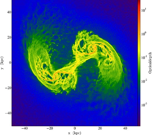
Dust optical depth at the CO J = 9-8 line for a simulated galaxy merger with ΣSFR comparable to Arp 220. Opacities are taken from Weingartner & Draine (2001). Even at the relatively long wavelength of ∼290 μm, the column densities are substantial enough that the lines suffer significant extinction.
4.4.3 Excitation by the microwave background
As shown in Fig. 4, the typical minimum temperature in GMCs is ∼ 8-10 K. In these low-density GMCs, this simply reflects the heating expected by cosmic rays with a Milky Way ionization rate. At redshifts z ≳ 3, however, the cosmic microwave background (CMB) temperature will exceed this – hence heating via this channel may be important. Because our simulations are not bona fide cosmological simulations, this effect thus far has been neglected.
In Fig. 12, we show the effects of explicitly including heating by the CMB on three simulated SLEDs for three galaxies with a large dynamic range in ΣSFR. These calculations include the effects of the CMB on both lines and dust, following the standard treatment in despotic – see Krumholz (2013) for details. The left-hand panel shows a model where the CMB is included with TCMB = 10.1 K (modelling the effects at z = 3), and the right-hand panel shows TCMB = 19.1 K (modelling the effects at z = 6). The dashed lines in each panel show our fiducial model with no CMB radiation included, while the solid lines show the impact of CMB variations.
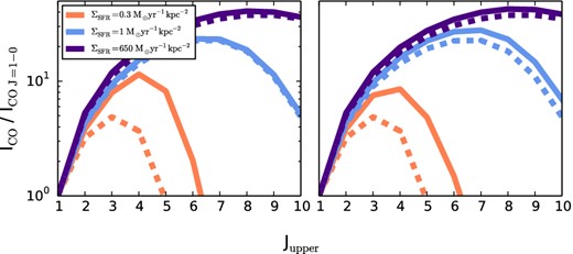
Effect of the CMB on the SLEDs of high-z galaxies. The left-hand panel shows a model where TCMB is scaled for z = 3, while the right-hand panel shows TCMB for z = 6. The dashed lines in each panel show our fiducial model (with no CMB radiation), while the solid lines show the effect of including the CMB. High-ΣSFR galaxies are only marginally affected by the high temperatures of the CMB at high z, while the lowest ΣSFR systems will show substantially more emission at high J, and a flattening of the SLED as the CMB temperature increases. Note that the effect of the CMB is only noticeable on galaxies that have substantially less ΣSFR than the typical star-forming galaxy detected at z ≳ 2.
The CMB has relatively minimal impact on the more intense star-forming galaxies. This is because the typical temperatures are already quite warm owing to an increased coupling efficiency between gas and dust, as well as increased cosmic ray heating. Lower ΣSFR galaxies show a larger difference when considering the CMB. The ∼10 K background at z = 3 drives more excitation at lower rotational levels (J = 2), while the ∼20 K background at z = 6 spreads the excitation to even higher levels (J = 5). The result is that at the highest redshifts, low-ΣSFR galaxies will have SLEDs that are flatter towards high J than what our fiducial model would predict.
This said, the effects of the CMB will be relatively minimal on any galaxies that have been detected in CO at high z thus far. As shown, only galaxies with relatively low ΣSFR ≲ 0.5 M⊙ yr−1 kpc−2 show a significant impact on the CO excitation from the CMB. This is roughly one order of magnitude lower SFR surface density than the typical BzK selected galaxy at z ∼ 2, and roughly three orders of magnitude lower than typical starbursts selected at z ∼ 6. Therefore, we conclude that the effect of CMB may drive deviations from our model in the observed SLED for low (ΣSFR ≲ 1 M⊙ yr−1 kpc−2) SFR surface density galaxies at high z, but that the effect is negligible for present high-z samples, and is likely to remain so for some time to come.
5 SUMMARY AND CONCLUSIONS
Observations of galaxies at low and high z show a diverse range of CO excitation ladders or SLEDs. In order to understand the origin of variations in galaxy SLEDs, we have combined a large suite of hydrodynamic simulations of idealized disc galaxies and galaxy mergers with molecular line radiative transfer calculations, and a fully self-consistent model for the thermal structure of the molecular ISM. Broadly, we find that the CO ladder can be relatively well parametrized by the galaxy-wide star formation rate surface density (ΣSFR).
We find that the CO excitation increases with increasing gas densities and temperatures, owing to increased collisions of CO with H2 molecules. The average gas density and temperature in the molecular ISM in turn increase with ΣSFR. As a result, the SLED rises at higher J’s in galaxies with higher SFR surface densities.
High SFR surface density galaxies tend to have increased line optical depths. This effect, which comes from the increased population of high-J levels, in turn drives down the effective density for thermalization of the high-J lines.
The gas temperature in extreme ΣSFR systems rises owing to an increase in cosmic ray ionization rates, as well as increased efficiency in gas–dust energy transfer. For Jupper ≲ 6, the lines tend to be in the Rayleigh–Jeans limit (Eupper ≪ kT), and once the density is high enough to thermalize the levels, this produces lines whose intensity ratios scale as J2. Lines arising from J ≳ 7, however, do not reach the Rayleigh–Jeans limit even for the most extreme SFRs currently detected, and thus the SLED is always flatter than J2 for J ≳ 7.
CO line ratios can be well parametrized by a power-law function of ΣSFR. We provide the parameter fits for both well-resolved observations and the more typical unresolved observations where the same emitting area is assumed for all lines (equation 19, and Tables 2 and 3). Our functional form for the CO line ratios quantitatively matches multi-line observations of both local and high-z galaxies over a large dynamic range of physical properties. In principle, this model can allow for the full reconstruction of a CO SLED with an arbitrary CO line detection (below Jupper ≤ 9) and a SFR surface density estimate.
DN thanks David Ballantyne, Tim Davis, Jackie Hodge, Tucker Jones, Padelis Papadopoulos, Naseem Rangwala, Dominik Riechers, Ian Smail and Mark Swinbank for helpful conversations, and Joe Cammisa for managing the Haverford College Cluster, where the simulations for this project were run. DN also thanks Matt Turk and Nathan Goldbaum, and the broader yt community and discussion boards for helpful conversations along the way regarding the yt data analysis package. The authors thank the anonymous referee for feedback that improved this work. The ideas for this work were developed at the Aspen Center for Physics. It is supported by the National Science Foundation grant no. PHY-1066293. DN acknowledges support from the NSF via grant AST-1009452. MRK acknowledges support from the NSF through grant AST-0955300 and NASA through ATP grant NNX13AB84G. This research made use of astropy, a community-developed core python package for Astronomy (Astropy Collaboration 2013), as well as the yt visualization and data analysis package (Turk et al. 2011). This research has made use of NASA's Astrophysics Data System Bibliographic Services.
We use this simplification to avoid having to iterate the Mach number, gas temperature, dust temperature, and level populations to convergence simultaneously, as this would be prohibitively expensive. The current calculation, using a fixed Mach number while iterating the gas and dust temperatures and level populations to convergence, is already quite expensive. The effect of assuming a fixed Mach number is fairly small in any event. The Mach number enters the calculation only through its effects on the median gas density used in calculations of the collisional excitation rates, so the main effect of a fully self-consistent treatment would be to lower the Mach number and thus the median gas density in the most vigorously star-forming galaxies where the molecular gas temperature exceeds 10 K. However, in these galaxies the density is so high that deviations from LTE are generally not very important, and would remain unimportant even with lower Mach numbers.
In Narayanan et al. (2011b), we explored models that included the effects of turbulent heating on molecular clouds via both adiabatic compression as well as viscous dissipation. These tests found only modest differences between our fiducial model and models that included turbulent heating.
It is worth noting that this definition does not include terms associated with stimulated emission, nor does it include collisional de-excitation to levels other than the J − 1 level. Both of these are sometimes included in the denominator when defining the critical density.
It is important to note that not all of the aforementioned drivers of enhanced gas density are causally correlated with increased SFR surface densities. For example, the calculation of internal GMC velocity dispersions (and resultant turbulent compression of gas) is done in post-processing, while the galaxy-wide SFRs are calculated on the fly in the hydrodynamic simulations. As a result, the two are not causal.
Though note that if differential magnification for the Cloverleaf is important, this may complicate the comparison.
In practice, in the Narayanan et al. (2011b, 2012a) studies, we utilized turtlebeach (Narayanan et al. 2006, 2008a) as the CO radiative transfer code, rather than despotic. However, since the core escape probability algorithms in turtlebeach are the same as in despotic, and very little non-local line coupling is expected on galaxy-wide scales, we expect the results to be nearly identical between the two.
