An explicit scheme for ohmic dissipation with smoothed particle magnetohydrodynamics

Tsukamoto, Yusuke; Iwasaki, Kazunari; Inutsuka, Shu-ichiro

doi:10.1093/mnras/stt1205

Abstract

In this paper, we present an explicit scheme for Ohmic dissipation with smoothed particle magnetohydrodynamics (SPMHD). We propose an SPH discretization of Ohmic dissipation and solve Ohmic dissipation part of induction equation with the super-time-stepping method (STS) which allows us to take a longer time step than Courant–Friedrich–Levy stability condition. Our scheme is second-order accurate in space and first-order accurate in time. Our numerical experiments show that optimal choice of the parameters of STS for Ohmic dissipation of SPMHD is ν_sts ∼ 0.01 and N_sts ∼ 5.

magnetic fields, MHD, methods: numerical, stars: formation, stars: protostars

INTRODUCTION

Magnetic field plays an important role in various astrophysical problems. In star formation processes, magnetic field changes the formation and evolution of protostars, discs and jets (e.g. Machida, Tomisaka & Matsumoto 2004; Matsumoto & Tomisaka 2004; Matsumoto 2007; Inutsuka, Machida & Matsumoto 2010; Machida, Inutsuka & Matsumoto 2011). Until recently, these interesting phenomena in collapsing magnetized cloud core have been investigated with nested-grid code or adaptive-mesh-refinement code.

Smoothed particle hydrodynamics (SPH) is a suitable numerical scheme for the protostellar collapse simulations because of its adaptive nature at high-density region and several authors have investigated the formation and evolution of protostar and disc in molecular cloud core (e.g. Bate 1998; Stamatellos, Whitworth & Hubber 2011; Tsukamoto & Machida 2011, 2013). In spite of the importance of magnetic field, however, most of the simulations with SPH do not include a magnetic field because, until recently, robust magnetohydrodynamic (MHD) schemes for SPH had not been developed.

Recently, several authors proposed robust smoothed particle magnetohydrodynamics (SPMHD) schemes. Tricco & Price (2012) proposed an SPMHD scheme with the hyperbolic divergence cleaning method (Dedner et al. 2002), which is originally proposed by Price & Monaghan (2005). They improved the original method of Price & Monaghan (2005) by changing discretization forms for ∇ · B and ∇ϕ. With this method, they successfully simulated protostellar collapse and formation of jets (see, also Price, Tricco & Bate 2012).

Iwasaki & Inutsuka (2011) proposed an SPMHD scheme based on Godunov SPH (GSPH) proposed by Inutsuka (2002). We refer to their method as Godunov SPMHD (GSPMHD). Instead of the artificial dissipation terms which are used in Price & Monaghan (2005), they use a solution of a non-linear Riemann problem with magnetic pressure and the method of characteristics to calculate the interactions between SPH particles. This method significantly reduces the numerical diffusion (compare fig. 2 of Iwasaki & Inutsuka 2011 and fig. 6 of Price & Monaghan 2005). They also have developed hyperbolic divergence cleaning method for GSPMHD (Iwasaki & Inutsuka, in preparation) and successfully simulated formation of jets (Iwasaki, in preparation).

In the previous studies about star formation processes with SPMHD, ideal MHD was assumed. But the assumption of ideality is generally not correct for the star formation processes because interstellar gas is partially ionized and several magnetic diffusion processes (e.g. Ohmic dissipation, Hall effect and ambipolar diffusion) play roles. Especially, Ohmic dissipation is effective at high- density region (ρ ≳ 10⁻¹² g cm⁻³) and formation and evolution of circumstellar discs, protostars and jets are significantly affected by Ohmic dissipation (see, e.g. Machida, Inutsuka & Matsumoto 2006).

To investigate the magnetic field in the intracluster medium of galaxy clusters, SPMHD simulations with Ohmic dissipation were performed by Bonafede et al. (2011). But they only considered the spatially constant magnetic resistivity. This assumption is generally not verified for protostellar collapse simulations because the resistivity has large spatial variation according to the gas density and temperature. Therefore, an Ohmic dissipation scheme for SPMHD which includes the effect of the spatially varying resistivity is desired to investigate formation and evolution of protostars, discs and jets.

In this paper, we propose a new explicit scheme for Ohmic dissipation with SPMHD. In Section 2, we describe our SPH discretization for Ohmic dissipation and time-stepping method. We present the results of several numerical tests in Section 3. Finally, we summarize our results in Section 4.

EXPLICIT SCHEME

Discretization

The induction equation with Ohmic dissipation is

\begin{eqnarray} \frac{{\rm d}(\boldsymbol {B}/\rho )}{{\rm d} t}=\frac{\boldsymbol {B}}{\rho }\cdot \nabla \boldsymbol {v} -\frac{1}{\rho }\nabla \times (\eta \nabla \times \boldsymbol {B}), \end{eqnarray}

(1)

where ρ, B, v, η denote the density, magnetic field, velocity and resistivity, respectively. Equation (1) is solved by an operator splitting approach and we focus on the solution of the second term on the right-hand side. The equation of Ohmic dissipation is given as

\begin{eqnarray} \frac{{\rm d} (\boldsymbol {B}/\rho )}{{\rm d} t}=-\frac{1}{\rho }\nabla \times (\eta \nabla \times \boldsymbol {B}). \end{eqnarray}

(2)

Equation (2) is written as

\begin{eqnarray} \frac{{\rm d} (B_\mu /\rho )}{{\rm d} t}=-\frac{1}{\rho } \left\lbrace \mathrm{\partial} _\nu (\eta \mathrm{\partial} _\mu B_\nu - \eta \mathrm{\partial} _\nu B_\mu ) \right\rbrace \equiv \frac{1}{\rho } \mathrm{\partial} _\nu F_{\mu \nu }. \end{eqnarray}

(3)

Here, we used Greek letter, μ, ν to denote the components of vector and we used Einstein summation convention. There are several choices for the discretization of the (∇ · F)/ρ. In this study, we adopted the following discretization. Discretization form of (∇ · F)/ρ of ith particle is

\begin{eqnarray} \left(\frac{1}{\rho }\mathrm{\partial} _\nu F_{\mu \nu } \right)_i &=& -\int \frac{\mathrm{\partial} _\nu (\eta \mathrm{\partial} _\mu B_\nu - \eta \mathrm{\partial} _\nu B_\mu )}{\rho }W_i \text{d}^3 r\nonumber\\ &=& \int \eta (\mathrm{\partial} _\mu B_\nu - \mathrm{\partial} _\nu B_\mu ) \mathrm{\partial} _\nu \left(\frac{ W_i}{\rho } \right)\text{d}^3 r \nonumber \\ & \sim & -\sum _j m_j \left\lbrace \frac{\eta _i(\mathrm{\partial} _\mu B_\nu -\mathrm{\partial} _\nu B_\mu )_i}{\rho _i^2}\right.\nonumber\\ &&+\left.\,\frac{\eta _j(\mathrm{\partial} _\mu B_\nu -\mathrm{\partial} _\nu B_\mu )_j}{\rho _j^2} \right\rbrace \mathrm{\partial} _\nu W_{ij}. \end{eqnarray}

(4)

Here, we used Latin letter, i, j to denote the particle number and W_i = W[x − x_i, h(x)] and |$W_{ij}=W[\boldsymbol {x_i}-\boldsymbol {x_j},\bar{h}_{ij}]$|⁠, where we adopted the mean smoothing length as |$\bar{h}_{ij}=(h_i+h_j)/2$|⁠.

We also investigated the following formula for (∇ · F)/ρ:

\begin{eqnarray} &&{\left(\frac{1}{\rho }\mathrm{\partial} _\nu F_{\mu \nu } \right)_i=}\nonumber\\ &&{\qquad -\, \sum _j m_j\left[ 4 \frac{1}{\rho _i\rho _j}\frac{(\eta _i\eta _j)}{(\eta _i+\eta _j)}\frac{(B_{\mu ,j}-B_{\mu ,i})}{|\boldsymbol {x_{ij}}|^2}(x_{\nu ,i}-x_{\nu ,j})\mathrm{\partial} _\nu W_{ij}\right.}\nonumber\\ &&{\qquad +\, \left.\left\lbrace \frac{\eta _i(\mathrm{\partial} _\mu B_\nu )_i}{\rho _i^2} +\frac{\eta _j(\mathrm{\partial} _\mu B_\nu )_j}{\rho _j^2}\right\rbrace \mathrm{\partial} _\nu W_{ij}\right].} \end{eqnarray}

(5)

The discretization of the first term on the right-hand side is suggested by Cleary & Monaghan (1999). The spatial resolution of this formula is slightly better than that of equation (4) but this introduces larger divergence error because the discretizations of the derivative of the magnetic field and the volume factor are inconsistent between the first and the second term. Therefore, we adopted equation (4).

There are also several choices for the gradient tensor of magnetic field. In the following test calculations, we adopted

\begin{eqnarray} (\nabla \boldsymbol {B})_i=\frac{1}{\rho _i}\sum _j m_j(\boldsymbol {B}_j-\boldsymbol {B}_i)\nabla W[\boldsymbol {x_i}-\boldsymbol {x_j},h_i]. \end{eqnarray}

(6)

We use the cubic spline kernel of Monaghan & Lattanzio (1985),

\begin{eqnarray} W(r,h) = C_{\rm f} \left\lbrace \begin{array}{ll}1 - \frac{3}{2} q^2 + \frac{3}{4} q^3, & \quad 0 \le q < 1 \\ \frac{1}{4}(2-q)^3, & \quad 1 \le q < 2 \\ 0 & \quad 2< q \end{array} \right. \end{eqnarray}

(7)

where q = r/h and |$C_{\rm f}=\frac{1}{\pi h^3},\ \frac{10}{7\pi h^2}$| for three and two dimensions, respectively. The smoothing length of ith particle is determined iteratively by the relation

\begin{eqnarray} h_i=C_{\rm h}\left(\frac{m}{\rho _i}\right)^{1/d}, \end{eqnarray}

(8)

where d is the dimension of the problem. C_h is a parameter and set to be 1.2.

Although, we do not solve the energy equation in the following test calculations, it would be useful to derive the SPH discretization of Ohmic dissipation term in the energy equation. The energy equation of Ohmic dissipation is given as

\begin{eqnarray} \frac{\text{D} e}{\text{D}t} \big \vert _{{\rm Ohm}}&=& \frac{1}{\rho } \nabla \cdot \lbrace \eta \boldsymbol {B} \times (\nabla \times \boldsymbol {B})\rbrace \nonumber\\ & =& \frac{1}{\rho } \nabla \cdot \left\lbrace \eta \nabla \left(\frac{\boldsymbol {B}^2}{2} \right) - \eta \boldsymbol {B}\cdot \nabla \boldsymbol {B} \right\rbrace \equiv \frac{1}{\rho } \nabla \cdot \boldsymbol {S}, \end{eqnarray}

(9)

where |$e=\frac{1}{2}{\boldsymbol v}^2+u+\frac{\boldsymbol {B}^2}{2\rho }$| is the specific total energy and u = P/[(γ − 1)ρ] is the specific internal energy. The discretization form of (∇ · S)/ρ of ith particle is

\begin{eqnarray} \left(\frac{1}{\rho }\mathrm{\partial} _\nu S_{\nu } \right)_i &=& \int \frac{\mathrm{\partial} _\nu S_\nu }{\rho }W_i \text{d}^3 r = -\int S_\nu \mathrm{\partial} _\nu \left(\frac{ W_i}{\rho } \right)\text{d}^3 r \nonumber \\ & \sim & \sum _j m_j \left\lbrace \frac{(S_\nu )_i}{\rho _i^2}+\frac{(S_\nu )_j}{\rho _j^2} \right\rbrace \mathrm{\partial} _\nu W_{ij}, \end{eqnarray}

(10)

where S_ν is calculated as

\begin{eqnarray} S_\nu \!=\eta \left\lbrace \mathrm{\partial} _\mu \left(\frac{B_\nu ^2}{2}\right) - B_\mu (\mathrm{\partial} _\mu B_\nu ) \right\rbrace \!=\eta \left\lbrace B_\nu (\mathrm{\partial} _\mu B_\nu ) - B_\mu (\mathrm{\partial} _\mu B_\nu ) \right\rbrace ,\nonumber\\ \end{eqnarray}

(11)

and equation (6). The equation (10) is antisymmetric under particle exchange and it is obvious that the error of the total energy is within machine epsilon by this discretization.

Time-stepping

During the protostellar collapse, high-density region ρ ≳ 10⁻¹⁰ g cm⁻³ appears. In the high-density region, the time-scale of Ohmic dissipation is shorter than the dynamical time-scale of the gas and the computational cost for Ohmic dissipation becomes large. To reduce the computational cost, we adopt the super-time-stepping method (STS) proposed by Alexiades, Amiez & Gremaud (1996). This method was used for Ohmic dissipation in Tomida et al. (2013) and ambipolar diffusion in Choi, Kim & Wiita (2009). In STS, Courant–Friedrich–Levy (CFL) stability condition is relaxed by requiring the stability not at the end of each time step but at the end of a cycle of N_sts steps. Following Alexiades et al. (1996), we define a super time step, |$\Delta T_{{\rm sts}} = \sum _{j=1}^{N_{{\rm sts}} } \tau _j$|⁠, where τ_j is the sub-step and is given as

\begin{eqnarray} \tau _j=\Delta t_{{\rm exp}}\left[(1-\nu _{{\rm sts}})\cos \left(\frac{2j-1}{N_{{\rm sts}}}\frac{\pi }{2}\right)+1+\nu _{{\rm sts}}\right]^{-1}. \end{eqnarray}

(12)

Thus, the super time step is

\begin{eqnarray} \Delta T_{{\rm sts}}=\sum _{j=1}^{N{{\rm sts}}} \tau _j=\Delta t_{{\rm exp}}\frac{N_{{\rm sts}}}{2\nu _{{\rm sts}}^{1/2}}\frac{\left(1+\nu _{{\rm sts}}^{1/2}\right)^{2N_{{\rm sts}}} -\left(1-\nu _{{\rm sts}}^{1/2}\right)^{2N_{{\rm sts}}}}{\left(1+\nu _{{\rm sts}}^{1/2}\right)^{2N_{{\rm sts}}} +\left(1-\nu _{{\rm sts}}^{1/2}\right)^{2N_{{\rm sts}}}},\nonumber\\ \end{eqnarray}

(13)

where Δt_exp is the explicit time step for Ohmic dissipation and we use Δt_exp = C_CFL h²/2η. Here, C_CFL is CFL number and h is the smoothing length. ν_sts is a parameter that controls the stability and the acceleration of the scheme. With smaller ν_sts, the scheme becomes faster but unstable. Optimal choice of ν_sts depends on the problem and we investigate the optimal choice for ν_sts in Section 3. With STS, magnetic field is updated as

\begin{eqnarray} \left(\frac{\boldsymbol {B}}{\rho }\right)\big \vert _{t+\Delta T_{{\rm sts}}}=\left(\frac{\boldsymbol {B}}{\rho }\right)\big \vert _{t} +\sum _{j=1}^{N_{{\rm sts}}}\tau _j\frac{{\rm d}(\boldsymbol {B}/\rho )}{{\rm d}t}\big \vert _{t+\sum _{k=0}^{j-1}\tau _k}. \end{eqnarray}

(14)

For comparison, we also performed simulations with a simple Euler method such as

\begin{eqnarray} \left(\frac{\boldsymbol {B}}{\rho }\right)\big \vert _{t+\Delta t_{{\rm exp}}}=\left(\frac{\boldsymbol {B}}{\rho }\right)\big \vert _{t} +\Delta t_{{\rm exp}}\frac{{\rm d}(\boldsymbol {B}/\rho )}{{\rm d}t}\big \vert _{t}. \end{eqnarray}

(15)

NUMERICAL TESTS

Sinusoidal diffusion problem

At first, we consider a simple problem in which sinusoidal magnetic field diffuses with a constant resistivity. The initial magnetic field is

\begin{eqnarray} B_x=0,\ B_y=0,\ B_z(x)=\sin (2\pi x). \end{eqnarray}

(16)

The resistivity is set to be η = 1. The computational domain is two dimensions and x, y ∈ [−0.5, 0.5]. We imposed periodic boundary conditions for each direction. We performed convergence tests by changing the time step Δt_exp and the smoothing length h. As a measure of the error, we calculated L₁ norm of B_z error, defined as

\begin{eqnarray} L_1=\frac{1}{N_{{\rm tot}}}\sum _i^{N_{{\rm tot}}}|B_{{\rm ref},\ z}(\boldsymbol {r}_i)-B_{z}(\boldsymbol {r}_i)|. \end{eqnarray}

(17)

As reference solutions, B_{ref, z}, we adopted the results with N_tot = 128², Δt_exp = 6 × 10⁻⁸ for the convergence test of the time step and N_tot = 256², Δt_exp = 1.5 × 10⁻⁶ for the convergence test of the smoothing length. For the calculations of both solutions, we used the Euler method. For STS, we adopted the value of ν_sts = 0.01, N_sts = 5.

Fig. 1 shows the L₁ norms as a function of time step. We show both results of Euler method (solid) and STS (dashed). The horizontal axis is Δt_exp for the Euler method and |$\bar{\tau }$| for STS. Here, |$\bar{\tau }$| is defined as |$\bar{\tau }=\sum _j^{N_{{\rm sts}}}\tau _j/N_{{\rm sts}}$|⁠. The figure shows that both schemes scale linearly and are of first order in time. This figure also shows that the error of STS is slightly larger than the Euler method at the same Δt. This means that, with the same computational cost, the error of STS is slightly larger than the Euler method. This is simply because the error of STS is proportional not to τ_j but to ΔT_sts.

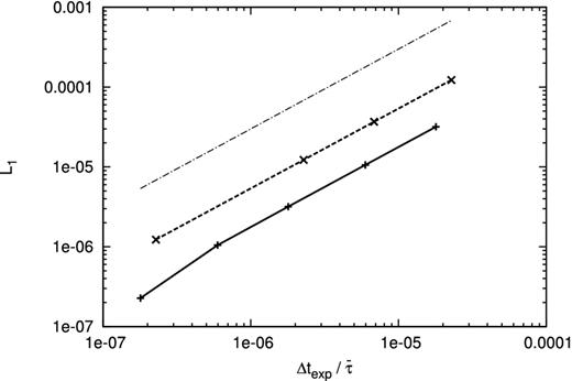
$L1 norm of error as a function of time step for the sinusoidal diffusion problem. Horizontal axis is Δtexp for the Euler method and $\bar{\tau }$ for STS. Solid line denotes the results with the Euler method and dashed line denotes the results with STS. The dash–dotted line is in proportion to Δt.$

Figure 1.

L₁ norm of error as a function of time step for the sinusoidal diffusion problem. Horizontal axis is Δt_exp for the Euler method and |$\bar{\tau }$| for STS. Solid line denotes the results with the Euler method and dashed line denotes the results with STS. The dash–dotted line is in proportion to Δt.

Open in new tab Download slide

Fig. 2 shows the L₁ norms as a function of smoothing length. The time step is fixed to be Δt_exp = 1.5 × 10⁻⁶ and the Euler method is used. The figure shows that the error is proportional to h² and it is confirmed that our discretization is of second order in space.

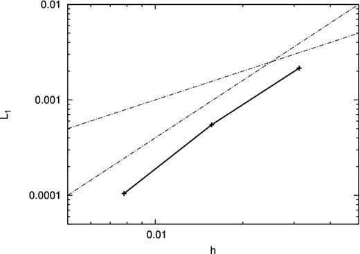
L1 norm of error as a function of smoothing length for the sinusoidal diffusion problem. Solid line denotes the results with the Euler method. The dash–dotted lines are in proportion to h and h2, respectively.

Figure 2.

L₁ norm of error as a function of smoothing length for the sinusoidal diffusion problem. Solid line denotes the results with the Euler method. The dash–dotted lines are in proportion to h and h², respectively.

Open in new tab Download slide

Gaussian diffusion problem

Next, we consider magnetic diffusion of B_z in Gaussian profile. The initial profile of magnetic field is given as

\begin{eqnarray} B_x=0,\ B_y=0,\ B_z(x,y)=\frac{1}{4\eta \pi t_0}\exp \left[-\frac{x^2+y^2}{4\eta t_0}\right], \end{eqnarray}

(18)

where t₀ is the initial time and set to be unity. We set magnetic resistivity as η = 1. The computational domain is two dimensions and x, y ∈ [−16, 16]. We impose periodic boundary conditions for each direction. The particle number for each direction is fixed to be 128.

Fig. 3 shows the L₁ norm as a function of time step at t = 8. Again, we considered both the Euler method (solid) and STS (dashed). The reference solution is the result with N_tot = 128², Δt_exp = 1.4 × 10⁻⁴ and the Euler method. The figure shows the same tendency of the results of sinusoidal diffusion problem, i.e. both schemes are of first order and the error of STS is slightly larger than the Euler method at the same time step.

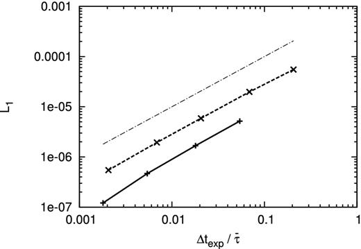
$L1 norm of error as a function of time step for the Gaussian diffusion problem. Horizontal axis is Δtexp for the Euler method and $\bar{\tau }$ for STS. Solid line denotes the results with the Euler method and dashed line denotes the results with STS. The dash–dotted line is in proportion to Δt.$

Figure 3.

L₁ norm of error as a function of time step for the Gaussian diffusion problem. Horizontal axis is Δt_exp for the Euler method and |$\bar{\tau }$| for STS. Solid line denotes the results with the Euler method and dashed line denotes the results with STS. The dash–dotted line is in proportion to Δt.

Open in new tab Download slide

To understand how the efficiency of STS depends on the parameters, we defined acceleration efficiency, F = ΔT_sts/(N_stsΔt_exp) and plotted it in Fig. 4 with ν_sts = 10⁻², 10⁻³, 10⁻⁴. The figure shows that the maximum of acceleration efficiency is determined by given ν_sts and the maximum value is |$F_{\text{max}}=1/\sqrt{\nu _{{\rm sts}}}$|⁠. Therefore, small ν_sts is preferable for the acceleration. But the small ν_sts makes the scheme unstable. This figure also shows the efficiency saturates around |$N_{{\rm sts}}\sim 1/\sqrt{\nu _{{\rm sts}}}$|⁠. Therefore, optimal choice of N_sts is |$\sim 1/\sqrt{\nu _{{\rm sts}}}$|⁠.

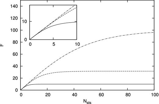
The acceleration efficiency, F = ΔTsts/(NstsΔtexp), as a function of Nsts for the case with νsts = 10−2 (solid), 10−3 (dashed), 10−4 (dash–dotted).

Figure 4.

The acceleration efficiency, F = ΔT_sts/(N_stsΔt_exp), as a function of N_sts for the case with ν_sts = 10⁻² (solid), 10⁻³ (dashed), 10⁻⁴ (dash–dotted).

Open in new tab Download slide

To seek the optimal choices of ν_sts and N_sts for Ohmic dissipation, we investigated the behaviour of the solutions at t = 8 by changing the parameters. We choose the parameter sets as ν_sts = (10⁻², 10⁻³, 10⁻⁴) and N_sts = 5, 10. The CFL number is set to be C_CFL = 0.3 for all calculations. The results at y = 0 are shown in Fig. 5. In this figure, only 64 particles are plotted to make the results more visible. The exact solution,

\begin{eqnarray} B_z(x,y)=\frac{1}{4\eta \pi (t_0+t)}\exp \left[-\frac{x^2+y^2}{4\eta (t_0+t)}\right], \end{eqnarray}

(19)

is also plotted. The results with N_sts = 5 (left-hand panel) and (ν_sts, N_sts) = (10⁻², 10) (circles in the right-hand panel) agree well with the exact solution. In the case of N_sts = 10, as ν_sts becomes small, the solution becomes distorted and the result with ν_sts = 10⁻⁴ shows the significant overshoot. This results shows that ν_sts ∼ 0.01 is preferable for the stability. From Fig. 4, we can see that F already saturates at N_sts ∼ 5 for ν_sts = 0.01. Therefore, we recommend ν_sts ∼ 0.01 and N_sts ∼ 5 as the optimal values of the parameters.

Figure 5.

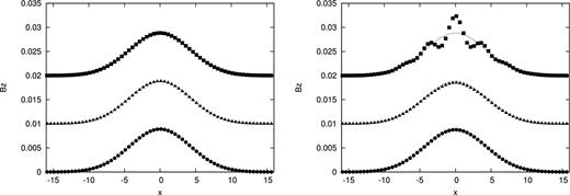
Profile of B_z at y = 0 plane at t = 8 of Gaussian diffusion problem. Circles, triangles, rectangles denote the results with ν_sts = 10⁻², 10⁻³, 10⁻⁴, respectively. Left- and right-hand panels show the results with N_sts = 5 and N_sts = 10, respectively. The dashed line denotes the exact solution at t = 8. Each solution is offset from each other by 0.01 in the vertical direction to make the results more visible.

Open in new tab Download slide

A test with spatially varying resistivity

In this subsection, we consider the diffusion of B_z in Gaussian profile with the spatially varying resistivity. The resistivity distribution is given as

\begin{eqnarray} \eta (\boldsymbol {r})=\exp \left[-(x^2+y^2+z^2)\right], \end{eqnarray}

(20)

and the initial magnetic field is

\begin{eqnarray} B_x=0,\ B_y=0,\ B_z(\boldsymbol {r})=\exp \left[-(x^2+y^2)\right]. \end{eqnarray}

(21)

The computational domain is three dimensions and x, y, z ∈ [−3, 3]. We impose periodic boundary conditions for each direction.

Fig. 6 shows the contour maps of B_x and B_z obtained at t = 1 with the Euler method with Δt_exp = 10⁻³ and STS with C_CFL = 0.3, ν_sts = 0.01, N_sts = 5. The particle number of each direction is 48. The results are consistent with each other and also consistent with the results calculated with the grid-code (see, Matsumoto 2011). But the B_z around the centre is slightly overestimated with STS.

Figure 6.

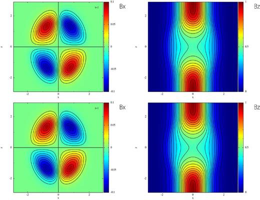
Magnetic field distributions of the 3D diffusion problem with spatially varying resistivity at t = 1. y = 0 planes are shown. The magnetic field is solved with the Euler method and Δt_exp = 10⁻³ for top panels and with STS and C_CFL = 0.3, ν_sts = 0.01, N_sts = 5 for bottom panels. Left-hand panels show B_x and contour levels are B_x = −0.09, −0.08, …, 0.09. Right-hand panels show B_z and contour levels are B_z = 0.05, 0.1, …, 0.95.

Open in new tab Download slide

To confirm that our discretization is of second order in space with the spatially varying resistivity, we show the L₁ norm of B_z at t = 1 as a function of smoothing length in Fig. 7. The solutions are obtained with the Euler method and Δt_exp = 10⁻³. The reference solution is the result with N_tot = 96³ and Δt_exp = 10⁻³.

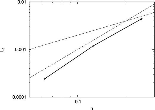
L1 norm of error as a function of smoothing length for the 3D diffusion problem with spatially varying resistivity at t = 1. Solid line denotes the results with the Euler method and Δtexp = 10−3. The dash–dotted lines are in proportion to h and h2, respectively.

Figure 7.

L₁ norm of error as a function of smoothing length for the 3D diffusion problem with spatially varying resistivity at t = 1. Solid line denotes the results with the Euler method and Δt_exp = 10⁻³. The dash–dotted lines are in proportion to h and h², respectively.

Open in new tab Download slide

This figure shows that the error is proportional to h² and it is confirmed that our discretization is of second order in space.

Gravitational collapse of magnetized cloud core

Finally, we consider the gravitational collapse of magnetized cloud core. The initial condition is as follows. The initial molecular cloud core has a mass of 1 M_⊙ and radius R_c = 2.7 × 10⁴ au. The free-fall time of the core is 2.4 × 10⁴ yr. The core is rigidly rotating with the angular velocity of Ω = 1.8 × 10⁻¹³ s⁻¹. For the boundary condition, we fix the particles whose radius is larger than 2.6 × 10⁴ au.

We adopt a barotropic equation of state

\begin{eqnarray} P = \left\lbrace \begin{array}{ll}c_{\rm s}^{2} \rho (1+(\rho /\rho _{\rm c})^{2/5}), & \quad \rho < \rho _{\rm d} \\ c_{\rm s}^{2} \rho _{\rm c} (\rho _{\rm d}/\rho _{\rm c})^{7/5} (\rho /\rho _{\rm d})^{1.1} & \quad \rho _{\rm d} \le \rho < \rho _{\rm e} \\ c_{\rm s}^{2} \rho _{\rm c} (\rho _{\rm d}/\rho _{\rm c})^{7/5} (\rho _{\rm e}/\rho _{\rm d})^{1.1}(\rho /\rho _{\rm e})^{5/3} & \quad \rho _{\rm e} \le \rho \end{array}\right., \end{eqnarray}

(22)

where c_s = 190 m s⁻¹, ρ_c = 4 × 10⁻¹⁴ g cm⁻³, ρ_d = 4 × 10⁻⁹ g cm⁻³ and ρ_e = 4 × 10⁻⁴ g cm⁻³. The initial magnetic field is parallel to the z-axis with the magnitude of B_z = 189 μG and the initial plasma beta is β = 2.5. The cloud core is modelled with 5 × 10⁶ particles.

We use the GSPMHD scheme of Iwasaki & Inutsuka (2011) with hyperbolic divergence cleaning method (Iwasaki & Inutsuka, in preparation) to solve ideal MHD part and Barnes–Hut tree algorithm with opening angle θ = 0.5 for gravity part. Ohmic dissipation is solved with present method. We adopted the resistivity η as

\begin{eqnarray} \eta = \frac{7.4 \times 10^5}{X_e}\sqrt{\frac{T}{10\, {\rm K}}} \left[ 1-{\rm tanh}\left( \frac{n}{10^{12}\,{\rm cm}^{-3} } \right) \right] \, \, \, {\rm cm}^2\,{\rm s}^{-1}, \end{eqnarray}

(23)

where T and n are the gas temperature and number density, and X_e is the ionization degree of the gas and

\begin{eqnarray} X_e = 5.7 \times 10^{-4} \left( \frac{n}{{\rm cm}^{-3}} \right)^{-1}. \end{eqnarray}

(24)

This model has the similar form to the model adopted in Machida, Inutsuka & Matsumoto (2007) but is artificially shifted to lower density to emphasize the effect of Ohmic dissipation in the first core. With our model, Ohmic dissipation is effective at 10⁻¹³ g cm⁻³ ≲ ρ ≲ 10⁻¹⁰ g cm⁻³.

In Fig. 8, the magnetic energy of the central part (the region of ρ > 0.1ρ_c, where ρ_c is the central or maximum density of the cloud core) normalized by the thermal energy as a function of central density is shown. The solid line and crosses show the results with the STS and Euler methods, respectively. The result of ideal MHD is also shown with the dashed line for comparison. The parameters for STS are ν_sts = 0.01, N_sts = 5.

Figure 8.

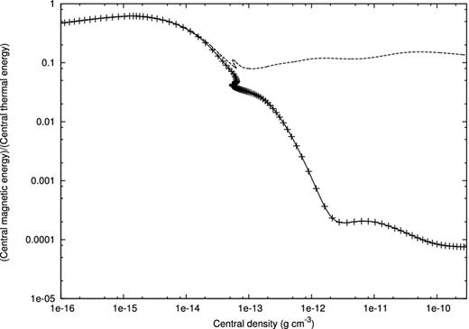
Central magnetic energy as a function of central density. The magnetic energy is normalized by the central thermal energy. Solid line and crosses denote the results of the resistive MHD model with the STS and Euler methods, respectively. The dashed line denotes the result of the ideal MHD model.

Open in new tab Download slide

When the central density is small (10⁻¹⁶ < ρ_c < 10⁻¹⁴ g cm⁻³), Ohmic dissipation is ineffective and there is no difference between resistive and ideal MHD models. The magnetic energy of the resistive MHD models begins to decrease at ρ_c ∼ 10⁻¹³ g cm⁻³ and becomes more than three orders of magnitude smaller than the ideal MHD model at ρ_c = 10⁻¹⁰ g cm⁻³. This figure also shows that the result with STS agree very well with that of the Euler method. Therefore, STS is proved to be beneficial for the realistic star formation problems.

In Fig. 9, the density distributions at the centre of the cloud when ρ_c ∼ 5 × 10⁻³ g cm⁻³ are shown, The velocity field is shown with red arrows.

Density distributions at the centre of the cloud of ideal MHD model (left) and resistive MHD model (right) when ρc ∼ 5 × 10−3 g cm−3. y = 0 planes are shown. The right-hand panel shows the result with STS. The parameters for STS are νsts = 0.01, Nsts = 5. The velocity field is shown with red arrows. The thin black lines show the density contour and the thick black line in left-hand panel shows the contour of |vz| = 0.

Figure 9.

Density distributions at the centre of the cloud of ideal MHD model (left) and resistive MHD model (right) when ρ_c ∼ 5 × 10⁻³ g cm⁻³. y = 0 planes are shown. The right-hand panel shows the result with STS. The parameters for STS are ν_sts = 0.01, N_sts = 5. The velocity field is shown with red arrows. The thin black lines show the density contour and the thick black line in left-hand panel shows the contour of |v_z| = 0.

Open in new tab Download slide

In the ideal MHD model (left), the black thick line denotes the velocity contour of |v_z| = 0. This line clearly shows that the outflow forms at the centre of the cloud. On the other hand, in the resistive MHD model (right), the outflow does not form because of the large resistivity in the first core. The structure of the first core is also very different from the ideal MHD model because the magnetic braking is ineffective. The detailed simulations and analysis of the formation and evolution of the outflow with ideal GSPMHD can be found in Iwasaki (in preparation).

SUMMARY AND PERSPECTIVE

In this paper, we presented an explicit scheme for Ohmic dissipation with SPMHD. We proposed a SPH discretization of Ohmic dissipation term in the induction equation. Ohmic dissipation part is solved with STS which relaxes the CFL stability condition requiring the numerical stability not at the end of each time step but at the end of a cycle of N_sts steps. Our scheme is second-order accurate in space and first-order accurate in time. The scheme successfully solves 2D and 3D tests. Our scheme is simple and can be easily implemented to any SPMHD codes.

We showed that STS introduces slightly larger error compared to the Euler method if we fix the computational costs. This comes from the fact that the error of STS is proportional not to τ but to ΔT_sts.

We found that optimal choice of the parameters of STS for Ohmic dissipation of SPMHD is ν_sts ∼ 0.01 and N_sts ∼ 5 and these values are consistent with the values suggested by Tomida et al. (2013).

Our present scheme is only first-order accurate in time. Recently, Meyer, Balsara & Aslam (2012) suggest a method which extends STS to second-order accurate in time. They applied this method to solve thermal conductivity. It is possible to solve Ohmic dissipation or other magnetic diffusion with their method. Note that, however, the efficiency of acceleration of their method is not so good as first-order STS at small N_sts and large N_sts is required to achieve better acceleration. We plan to improve accuracy in time of our scheme in future works.

We thank T. Matsumoto, M. N. Machida and T. Inoue for fruitful discussions. We also thank the referee, D. Price, for helpful comments. The snapshots were produced by splash (Price 2007). The computations were performed on XC30 system at CfCA of NAOJ and SR16000 at YITP in Kyoto University. YT and KI are financially supported by Research Fellowships of JSPS for Young Scientists.

REFERENCES

Alexiades

V.

Amiez

G.

Gremaud

P.-A.

,

Commun. Numer. Methods Eng.

,

1996

, vol.

12

pg.

31

Crossref

Search ADS

Bate

M. R.

,

ApJ

,

1998

, vol.

508

pg.

L95

Crossref

Search ADS

Bonafede

A.

Dolag

K.

Stasyszyn

F.

Murante

G.

Borgani

S.

,

MNRAS

,

2011

, vol.

418

pg.

2234

Crossref

Search ADS

Choi

E.

Kim

J.

Wiita

P. J.

,

ApJS

,

2009

, vol.

181

pg.

413

Crossref

Search ADS

Cleary

P. W.

Monaghan

J. J.

,

J. Comput. Phys.

,

1999

, vol.

148

pg.

227

Crossref

Search ADS

Dedner

A.

Kemm

F.

Kröner

D.

Munz

C.-D.

Schnitzer

T.

Wesenberg

M.

,

J. Comput. Phys.

,

2002

, vol.

175

pg.

645

Crossref

Search ADS

Inutsuka

S.-I.

,

J. Comput. Phys.

,

2002

, vol.

179

pg.

238

Crossref

Search ADS

Inutsuka

S.-i.

Machida

M. N.

Matsumoto

T.

,

ApJ

,

2010

, vol.

718

pg.

L58

Crossref

Search ADS

Iwasaki

K.

Inutsuka

S.-I.

,

MNRAS

,

2011

, vol.

418

pg.

1668

Crossref

Search ADS

Machida

M. N.

Tomisaka

K.

Matsumoto

T.

,

MNRAS

,

2004

, vol.

348

pg.

L1

Crossref

Search ADS

Machida

M. N.

Inutsuka

S.-i.

Matsumoto

T.

,

ApJ

,

2006

, vol.

647

pg.

L151

Crossref

Search ADS

Machida

M. N.

Inutsuka

S.-i.

Matsumoto

T.

,

ApJ

,

2007

, vol.

670

pg.

1198

Crossref

Search ADS

Machida

M. N.

Inutsuka

S.-i.

Matsumoto

T.

,

ApJ

,

2011

, vol.

729

pg.

42

Crossref

Search ADS

Matsumoto

T.

,

PASJ

,

2007

, vol.

59

pg.

905

Matsumoto

T.

,

PASJ

,

2011

, vol.

63

pg.

317

Matsumoto

T.

Tomisaka

K.

,

ApJ

,

2004

, vol.

616

pg.

266

Crossref

Search ADS

Meyer

C. D.

Balsara

D. S.

Aslam

T. D.

,

MNRAS

,

2012

, vol.

422

pg.

2102

Crossref

Search ADS

Monaghan

J. J.

Lattanzio

J. C.

,

A&A

,

1985

, vol.

149

pg.

135

Price

D. J.

,

PASA

,

2007

, vol.

24

pg.

159

Crossref

Search ADS

Price

D. J.

Monaghan

J. J.

,

MNRAS

,

2005

, vol.

364

pg.

384

Crossref

Search ADS

Price

D. J.

Tricco

T. S.

Bate

M. R.

,

MNRAS

,

2012

, vol.

423

pg.

L45

Crossref

Search ADS

Stamatellos

D.

Whitworth

A. P.

Hubber

D. A.

,

ApJ

,

2011

, vol.

730

pg.

32

Crossref

Search ADS

Tomida

K.

Tomisaka

K.

Matsumoto

T.

Hori

Y.

Okuzumi

S.

Machida

M. N.

Saigo

K.

,

ApJ

,

2013

, vol.

763

pg.

6

Crossref

Search ADS

Tricco

T. S.

Price

D. J.

,

J. Comput. Phys.

,

2012

, vol.

231

pg.

7214

Crossref

Search ADS

Tsukamoto

Y.

Machida

M. N.

,

MNRAS

,

2011

, vol.

416

pg.

591

Tsukamoto

Y.

Machida

M. N.

,

MNRAS

,

2013

, vol.

428

pg.

1321

Crossref

Search ADS

Download all slides

Month:	Total Views:
February 2017	2
March 2017	2
June 2017	9
August 2017	3
September 2017	4
October 2017	4
December 2017	2
January 2018	6
February 2018	6
March 2018	9
April 2018	7
May 2018	5
June 2018	13
July 2018	7
August 2018	9
September 2018	1
October 2018	2
November 2018	5
December 2018	7
January 2019	2
February 2019	7
March 2019	8
April 2019	13
May 2019	12
June 2019	11
July 2019	10
August 2019	5
September 2019	3
October 2019	6
November 2019	7
December 2019	9
January 2020	12
February 2020	3
March 2020	6
April 2020	3
May 2020	4
June 2020	8
July 2020	7
August 2020	4
September 2020	8
October 2020	2
November 2020	3
December 2020	2
January 2021	3
February 2021	9
March 2021	6
April 2021	9
May 2021	3
June 2021	10
July 2021	3
August 2021	4
September 2021	3
October 2021	8
November 2021	6
January 2022	5
February 2022	13
March 2022	1
April 2022	12
May 2022	14
June 2022	2
July 2022	23
August 2022	11
September 2022	9
October 2022	9
November 2022	2
December 2022	6
January 2023	2
February 2023	2
March 2023	2
April 2023	8
May 2023	7
June 2023	4
July 2023	6
August 2023	5
September 2023	1
October 2023	6
November 2023	4
December 2023	10
January 2024	10
February 2024	6
March 2024	9
April 2024	9
May 2024	9
June 2024	7
July 2024	13
August 2024	7
September 2024	7
October 2024	10
November 2024	3
December 2024	8
January 2025	19
February 2025	4
March 2025	7
April 2025	3

Article Contents

An explicit scheme for ohmic dissipation with smoothed particle magnetohydrodynamics

Abstract

INTRODUCTION

EXPLICIT SCHEME

Discretization

Time-stepping

NUMERICAL TESTS

Sinusoidal diffusion problem

Gaussian diffusion problem

A test with spatially varying resistivity

Gravitational collapse of magnetized cloud core

SUMMARY AND PERSPECTIVE

REFERENCES

Citations

Views

Altmetric

Email alerts

Astrophysics Data System

Citing articles via

Latest

Most Read

Most Cited

Article Contents

An explicit scheme for ohmic dissipation with smoothed particle magnetohydrodynamics

Abstract

INTRODUCTION

EXPLICIT SCHEME

Discretization

Time-stepping

NUMERICAL TESTS

Sinusoidal diffusion problem

Gaussian diffusion problem

A test with spatially varying resistivity

Gravitational collapse of magnetized cloud core

SUMMARY AND PERSPECTIVE

REFERENCES

Citations

Views

Altmetric

Email alerts

Astrophysics Data System

Citing articles via

Latest

Most Read

Most Cited

This Feature Is Available To Subscribers Only