


Abstract
Natural selection leaves a spatial pattern along the genome, with a haplotype distribution distortion near the selected locus that fades with distance. Evaluating the spatial signal of a population-genetic summary statistic across the genome allows for patterns of natural selection to be distinguished from neutrality. Considering the genomic spatial distribution of multiple summary statistics is expected to aid in uncovering subtle signatures of selection. In recent years, numerous methods have been devised that consider genomic spatial distributions across summary statistics, utilizing both classical machine learning and deep learning architectures. However, better predictions may be attainable by improving the way in which features are extracted from these summary statistics. We apply wavelet transform, multitaper spectral analysis, and S-transform to summary statistic arrays to achieve this goal. Each analysis method converts one-dimensional summary statistic arrays to two-dimensional images of spectral analysis, allowing simultaneous temporal and spectral assessment. We feed these images into convolutional neural networks and consider combining models using ensemble stacking. Our modeling framework achieves high accuracy and power across a diverse set of evolutionary settings, including population size changes and test sets of varying sweep strength, softness, and timing. A scan of central European whole-genome sequences recapitulated well-established sweep candidates and predicted novel cancer-associated genes as sweeps with high support. Given that this modeling framework is also robust to missing genomic segments, we believe that it will represent a welcome addition to the population-genomic toolkit for learning about adaptive processes from genomic data.
Introduction
A number of phenomena shape genomic diversity, including nonadaptive processes, such as mutation, recombination, genetic drift, and migration as well as adaptive processes, such as positive, negative, and balancing selection (Gillespie 2004). Many of these events leave local footprints of altered haplotypic variation across individuals in populations, restructuring the landscape of diversity across the genome (Fay et al. 2001; Prezeworski et al. 2005; Charlesworth 2006; Schlamp et al. 2016). To learn about such processes, myriad summary statistics have been developed over decades, providing tools for testing whether patterns in genetic variation match expectations, either from theoretical models or from mean patterns observed from simulations (e.g., Tajima 1983; Garud et al. 2015). One of the most extensively studied population-genetic phenomena that has received substantial attention in terms of method development over the past few decades is natural selection.
Natural selection is a process that acts on traits of individuals within an environment, leading to differential fitness among individuals that may result in changes in the frequencies of alleles that code for such traits within a population (Gillespie 2004). Genomic studies of a wide range of populations and species have been analyzed using a variety of summary statistic methodologies to search for signatures of natural selection (e.g., Glinka et al. 2003; Lucas et al. 2019; Xue et al. 2021). Summary statistics developed throughout the past several years rely heavily on the haplotype frequency spectrum (e.g., Garud et al. 2015), whereas more classical summaries focused more on the site frequency spectrum (e.g., Tajima 1983). These varied approaches interrogate different aspects of genomic variation, and lend greater ability to detect specific forms of adaptation (Vitti et al. 2013).
However, such summary statistics typically make simplifying assumptions about expected patterns of variation, and can be both underpowered and nonrobust to confounding factors when applied individually. To overcome the pitfalls associated with using a single summary statistic to uncover signals of evolutionary processes, combining the knowledge garnered from a plethora of summary statistics has become an emerging trend (Schrider and Kern 2018). Specifically, the recent expansion of modeling frameworks that combine sets of measured values to discriminate among diverse evolutionary scenarios is owed to the advancement of computational technologies and resurgence of statistical machine learning and artificial intelligence.
The goal of supervised machine learning is to provide algorithms with a dataset of known input (feature) and output (response) values, with the goal to learn the relationship (or function) that maps measured features to a given response (Hastie et al. 2009). This learned function is the model, and the shape of the function is estimated (trained) from the dataset of input and output examples, termed the training set. This model can then be deployed to make predictions on new input data. The taxonomy of supervised learning algorithms can be further split into regression and classification tasks, which depend on whether the response is a quantitative (regression) or qualitative (classification) value (Hastie et al. 2009). Different machine learning algorithms make varying assumptions regarding the form of this function, which ultimately influences the predictive accuracy of the trained models. Commonly employed supervised machine learning methods include linear regression (Weisberg 2005), logistic regression (Kleinbaum et al. 2002), decision trees (Safavian and Landgrebe 1991), random forests (Breiman 2001), support vector machines (Hearst et al. 1998), and neural networks (Müller et al. 1995).
The predictive models based on the application of supervised machine learning to problems in evolutionary genomics have been shown to typically offer greater detection power and accuracy, while also combating the drawbacks of individual hand-engineered summary statistics (e.g., Lin et al. 2011; Schrider and Kern 2016; Sheehan and Song 2016; Kern and Schrider 2018; Sugden et al. 2018; Mughal and DeGiorgio 2019; Mughal et al. 2020). These machine learning techniques employ diverse modeling paradigms, and have differing performances and robustness to confounding factors depending on how the data are modeled as well as the types of summary statistics that are used as input to the models. Thus, all methods show room for improvement in prediction performance.
To glean more information from input summary statistics, many of these models (e.g., Lin et al. 2011; Schrider and Kern 2016; Sheehan and Song 2016) construct feature sets so that they capture the expected spatial autocorrelation of variation in a local genomic region. That is, the input summary statistics are calculated over a number of contiguous or overlapping genomic windows with the hope that the machine learning models will discover relationships among various statistics calculated across different windows to aid in prediction. However, explicitly modeling these autocorrelations may have the potential for improving prediction performance. As an example, Mughal et al. (2020) developed a method for learning about positive natural selection by utilizing multiple summary statistics computed in overlapping genomic windows as input, and then modeled the autocorrelation across these windows by estimating the underlying continuous functional form of each summary statistic. Specifically, Mughal et al. (2020) employed a spectral analysis technique termed the discrete wavelet transform, which decomposed the summary statistic vectors in the form of multilevel details of constituent low- and high-frequency regions, enabling additional meaningful information to be extracted from the summary statistics.
Spectral analysis of signals has been extensively applied in various domains, including biomedical sciences (O’Brien et al. 2019), power systems (Khan and Pierre 2018), and seismography (Puryear et al. 2012), to extract information about the source (or process) responsible for the generation of the examined signals from their oscillatory characteristics. One way to extract information from the signal is to divide the signal into time-localized components and examine each part of the signal independently though spectra. Different spectral analysis methods focus on different characteristics of a signal (Xiang and Hu 2012), and thus, images of the characteristics identified by different spectral analysis methods can be used as input to established modeling frameworks that are able to extract meaningful information and make accurate predictions. One mechanism for attempting to learn such features is with supervised machine learning models known as convolutional neural networks (CNNs, LeCun et al. 1998).
Neural networks are a class of machine learning architectures that are inspired by the structure and function of the human brain. They consist of layers of interconnected nodes termed neurons, which process information in a way that is similar to how neurons in the brain process information. Such models can be used for a wide range of predictive modeling tasks that involve large amounts of data and complex relationships between the measured features and a predicted response. CNNs are a subclass of neural networks architectures that are effective for applications requiring image recognition and processing.
Multilayered CNNs process data in a hierarchical fashion through a network of nodes. When the input is an image, the first layer can identify simple features, such as edges and corners of objects in the image, whereas successive layers may identify more complicated features, such as shapes or higher-order objects, by building upon features learned from previous layers (LeCun et al. 1998). The final layer of the CNN makes a prediction using the identified features from the input image. To learn features from input images, CNNs rely on convolutions, which involve sliding a filter of a given size over the image and computing the dot product between the filter and each matching patch of pixels in the image (LeCun et al. 1998). Through this process, the network is able to identify invariant local patterns and features. Other layers, including pooling layers and activation layers, are also used in CNNs. Downsampling the output of the convolutional layers with pooling layers makes feature maps more precise, invariant to object orientation, and robust to noise, as well as makes the network more accurate. Networks learn more complicated relationships between features and the response through activation layers, which introduce nonlinearity to the network (LeCun et al. 1998). In the field of image recognition, CNNs have proven to be highly effective, often outperforming human experts on a variety of classification tasks (De Man et al. 2019).
CNNs offer a framework for extracting features from inputs that can be one-dimensional vectors, two-dimensional matrices (or grayscale images), and three-dimensional tensors (or color images) (LeCun et al. 1998). Several studies have shown the effectiveness of CNNs for detecting evolutionary events for both one- and two-dimensional signals (Schrider and Kern 2016; Flagel et al. 2019; Torada et al. 2019; Gower et al. 2021). Indeed, CNNs have been applied in the context of learning about evolutionary processes from image representations of haplotype variation, and have been demonstrated to often have greater power and accuracy compared to the current state-of-the-art summary statistic-based methods (Flagel et al. 2019; Isildak et al. 2021). A hybrid application of using two-dimensional spectra generated through signal decomposition to train CNNs has the potential to empower the CNNs to make more effective predictive models. To employ this modeling strategy, one-dimensional summary statistic signals need to be converted into two-dimensional spectra (Cohen 1995; Sejdi et al. 2009), which provide information about the spectral estimates of the underlying source (or process) that generates genomic variation.
Therefore, we seek to improve evolutionary process classifiers, by adding a layer of spectral inference of the underlying process generating the genetic variation. To that end, we use the detection of positive natural selection as a test case, as this setting is where the majority of population-genetic machine learning development has focused, and thus represents a test case for illustrating the performance gains by modeling input data differently. Positive natural selection increases the frequencies of alleles in a population that code for beneficial traits, potentially leading to fixation within the population and ultimately reducing diversity at the selected locus (Gillespie 2004). As this beneficial allele increases in frequency, alleles on the same haplotype at nearby neutral loci also increase in frequency through a process known as genetic hitchhiking (Smith and Haigh 1974). The resulting loss of haplotypic diversity around the selected locus is known as a selective sweep (Przeworski 2002; Hermisson and Pennings 2005), and is a footprint that is often used to uncover signals of past positive selection. Depending on the number of distinct haplotypes that have risen to high frequency, selective sweeps can be categorized as either soft or hard, with hard sweeps typically easier to detect due to their more conspicuous genomic pattern (Przeworski 2002; Hermisson and Pennings 2005; Garud et al. 2015).
In this article, we examine the utility of applying three signal decomposition methods on arrays of summary statistics computed across overlapping windows to generate spectra (Thomson 1982; Daubechies 1992; Stockwell et al. 1996), and develop machine learning methods trained with these images. We additionally employ ensemble-based stacking procedures (Hastie et al. 2009) that aggregate the results of individual classifiers with the goal of further improving power and accuracy to detect sweeps from genome variation. With this in mind, we introduce an approach termed SISSSCO (Spectral Inference of Summary Statistic Signals using COnvolutional neural networks) with open-source implementation available at https://www.github.com/sandipanpaul06/SISSSCO. As an empirical test case, we then apply our trained SISSSCO models to whole-genome data of the well-studied central European human individuals sequenced by the 1000 Genomes Project (The 1000 Genomes Project Consortium 2015). SISSSCO identifies multiple genes, including LCT, ABCA12, SLC45A2, HLA-DRB6, and HCG9, which have been identified as sweep candidates from previous studies. SISSSCO also identified several novel sweep candidates, including PDPN, WASF2, LRIG2, and SDAD1.
Results
In this section, we begin by highlighting power and accuracy to detect selective sweeps using various strategies that combine different spectral decompositions of summary statistic signals as well as stacking of trained CNN architectures. We also compare the performance of these approaches with other contemporary machine learning methods that take summary statistics as input to detect sweeps. We then investigate how confounding factors, like changing population sizes over time, the existence of missing genomic segments, and background selection, influence predictive accuracy, power, and robustness. Finally, as a proof of concept, we test our new approaches using a genomic dataset from a human population that has been extensively studied.
Modeling Description
To train and test our models, we simulated neutral and sweep replicate observations using the coalescent simulator discoal (Kern and Schrider 2016) under either an equilibrium constant-size demographic history of 10,000 diploid individuals (Takahata 1993) or under a nonequilibrium history inferred from central European human genomes (Terhorst et al. 2017) that includes a recent severe population bottleneck. Per-site per-generation mutation () and recombination rates (exponential distribution with mean and truncated at ) were chosen to reflect expectations from human genomes and previous studies (Payseur and Nachman 2000; Scally and Durbin 2012; Schrider and Kern 2016). For each simulated replicate, we sampled 198 haplotypes of length 1.1 megabase (Mb) to match the number of sampled haplotypes in our empirical experiments.
At the center of simulated sequences for sweep observations, we introduced a beneficial mutation that became selected for at a frequency of (drawn uniformly at random on a logarithmic scale) with per-generation selection coefficient (drawn uniformly at random on a logarithmic scale) and became fixed in the population t generations prior to sampling. For each of the two demographic scenarios, we generated two datasets: one with the sweep completing at time of sampling ( generations) and a setting that should be more difficult to distinguish from neutrality, with [0, 1,200] generations drawn uniformly at random, permitting the processes of mutation, recombination, and genetic drift to erode genomic footprints of the selective sweep after fixation. We denote these four datasets as Equilibrium_fixed, Equilibrium_variable, Nonequilibrium_fixed, and Nonequilibrium_variable, where the demographic history is given by either equilibrium (constant-size) or nonequilibrium (European human bottleneck), and the time of sampling after sweep completion is given by either as a fixed () or variable ([0, 1,200]) number of generations.
For each class (neutral or sweep), we generated 11,000 independent simulated replicate observations, with 9,000, 1,000, and 1,000 observations reserved for training, validation, and testing. For each replicate, we computed summary statistics across the simulated sequence to obtain nine one-dimensional signals to use as features for downstream modeling identical to the ones used in Mughal et al. (2020) (see Methods for summary statistic computation on simulated data). The initial summary statistic that we explored in our model training is the mean pairwise sequence difference (; Tajima 1983) estimated across sampled haplotypes. The dataset containing instances of computed as a one-dimensional signal of length 128 across a genomic sequence of neutral and selective sweep regions was used to test the efficacy of each of the three spectral analysis methods. These summary statistic signals of length 128 are based on short overlapping windows with a fixed number of single nucleotide polymorphisms (SNPs) per window, and a fixed SNP stride between windows (see Methods section). We calculated in overlapping windows with a goal to capture local patterns along a chromosome (see Methods section for details).
The two-dimensional images that we obtain by performing spectral analysis on a one-dimensional signal (e.g., ) are then fed into a CNN (LeCun et al. 1998), which is depicted in figure 1. The CNN has an input size of containing N training observations of c different summary statistic signals decomposed as images through spectral analysis. Here we have , , and . As we are currently only considering a single signal based on the statistic, we are using a channel input for our CNN. The CNN has two convolution layers with 32 filters, kernels of size (Agrawal and Mittal 2020), and a stride of two (Kong and Lucey 2017) with zero padding (Hashemi 2019). Each convolution layer is then followed by an activation layer using a rectified linear unit (ReLU), as well as a batch normalizing layer (Goodfellow et al. 2016). The convolution layers are followed by a dense layer containing 128 nodes, which is the same as the input signal length n. The dense layer also contains an elastic-net style regularization penalty (Zou and Hastie 2005), whereby network weights shrink in magnitude together toward zero through an -norm penalty while simultaneously performing feature selection by setting some weights to zero through an -norm penalty (Hastie et al. 2009). The fraction of regularization deriving from the -norm penalty is controlled by hyperparameter and the amount of total regularization is controlled by hyperparameter . The model also utilizes a dropout layer with dropout rate hyperparameter to further prevent model overfitting by reaching a saturation point (Srivastava et al. 2014; Goodfellow et al. 2016). The model is trained with each hyperparameter triple, with a batch size of 50 for 30 iterations, and the best model is chosen as the one with the smallest validation loss, where we employ the categorical cross-entropy loss measurement. We deployed the keras Python library (Chollet et al. 2015) with a TensorFlow (Abadi et al. 2015) back-end for training of CNNs and making downstream predictions from the learned models.
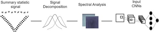
Depiction of a channel convolutional neural network (CNN) architecture. A summary statistic signal of length is used as input to a spectral analysis method (either wavelet decomposition, multitaper analysis, or S-transform) to decompose the signal into a matrix of dimensions , with , which is then standardized at each element based on the mean and standard deviation across all training observations, and is then used as input to a CNN. The CNN has two convolution layers (three layers for the S-transform), followed by a dense layer with n nodes containing both elastic-net and dropout regularization. The output layer of the CNN is a softmax that computes the probability of a sweep.
The first of three spectral analysis methods that we consider is wavelet decomposition. Specifically, we assume that each sequence of length represents a sample from a continuous wavelet containing n data points. This signal is then decomposed by a level m wavelet analysis method, with the Morlet wavelet (Bernardino and Santos-Victor 2005) selected as the mother wavelet. Level is chosen for the scalograms generated to match the size of the spectral images that result from the other two spectral analysis methods that we subsequently introduce. Every decomposed signal generates an dimensional scalogram matrix. A more detailed treatment of the wavelet decomposition for spectral analysis is provided in the Methods section, and we employed the PyWavelets Python package (Lee et al. 2019) to construct scalogram images.
Next, for the multitaper spectral analysis approach, to derive the periodogram of the estimate of the true power spectral density from a signal of size using the multitaper spectral analysis method, we used a window length of n. We calculated discrete prolate spheroidal sequence (DPSS) tapers over time half-bandwidth parameter () values in and a DPSS window size of , which results in a matrix of tapering windows of size and a vector of eigenvalues of length m. Here, is the bandwidth of the most dominant frequencies in the frequency domain such that . Using this matrix and vector, a periodogram of size is generated, which is the same as the dimension of the scalogram that we considered with the wavelet analysis method. See the Methods section for a complete detailed description of multitaper analysis. We utilized the spectrum Python package (Cokelaer and Hasch 2017) to generate multitaper periodogram images.
Finally, for spectral analysis using the Stockwell transform (also known as the S-transform) we used the same datasets as the previous two spectral analysis approaches. The S-transform returns a spectrogram matrix estimate of the true power spectral density that has size , where and where the length of the signal is . The spectrogram has the same image size as the previous two methods. See the Methods section for further details on the S-transform. We used the stockwell Python package (Satriano 2017) to estimate S-transform spectral images. The images are then fed into a CNN with identical architecture to that of the previous two methods with the addition of a third convolution layer, which we included as we found that adding this extra convolution layer substantially increased performance under the S-transform image inputs.
Application of Signal Decomposition
Supplementary figure S1, Supplementary Material online presents heatmaps of the raw spectral images, averaged across simulated replicates, for neutral and selective sweep regions using three signal decomposition methods. However, based on these raw images, it is difficult to visually distinguish between sweeps and neutrality for each of the spectral analysis methods. To better explore the visual differences within these matrices, we scaled each element of each spectral analysis matrix to have unit standard deviation across the neutral and sweep replicates. The mean scaled matrices depicted in figure 2 show the emergence of more-readily distinguishable patterns between sweeps and neutrality. The wavelet decomposition results display a clear distinction between the two classes, with a triangular bulge in the mid-segment of the sweep scalogram that is not present within the neutral scalogram. This pattern indicates that the selective sweep signals have information in the middle windows between windows 45 and 85 that is not present in neutral signals. Similarly, the mean sweep spectrogram generated by S-transform shows a T-shaped construct in the midportion of the image, again indicating a difference of power between the classes of some low- to mid-frequency components in the central windows. The mean spectra generated by multitaper analysis depict a rib-cage like structure in the mean sweep periodogram. Each ‘rib’ represents a Fourier transformation of a signal tapered by a single taper. The frequency of the taper increases as we descend the rows of the image, whereas the amplitude of the central window of the taper decreases. Hence, a signal tapered by higher frequency tapers generate a distorted representation of the signal. As the frequencies of the tapers increase, more low- and high-frequency components in the sweep signal are lost, resulting in a narrower spectral density. These characteristics of the tapers lead to the the rib-cage structure depicted in the mean sweep image.
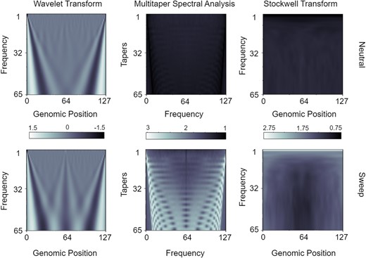
Mean spectral analysis input matrices for windows of the mean pairwise sequence differences across the neutral and sweep replicates under the Equilibrium_fixed dataset containing an equilibrium constant-size demographic history and a sweep that completed generations before sampling. Top row are neutral simulations and bottom row are sweep simulations. Spectral methods are depicted from left to right columns for the wavelet decomposition, multitaper analysis, and the S-transform, respectively. Elements of each matrix have been scaled to have a standard deviation of one across all N simulated replicates for a given spectral analysis method.
The standardized (combined centering and scaling) images in supplementary figure S2, Supplementary Materialonline that are ultimately used as input to CNNs show that the classes can be easily visually differentiated as the images show exactly opposite patterns for the two classes, with the images for neutral regions having lower values for the majority of the area in the images. These opposite patterns are due to centering. A peach pit shape is present in the center of both mean sweep and neutral spectrograms generated by the S-transform, albeit represented by two distinctly different shades corresponding to positive and negative values, respectively. Several mid- and low-frequency components are present in the central windows of the sweep samples, which results in the bright core of the peach pit in the mean sweep image. The rib-cage structure is also present in mean spectra of both classes in the images created by multitaper analysis, with different shades for the two classes corresponding mostly to positive and negative values.
Figure 2, supplementary figures S1 and S2, Supplementary Material online highlight the qualitative patterns in images derived from neutral and sweep settings that result from three different spectral analysis methods applied to a sequence of values calculated across overlapping genomic windows. Given that these images show qualitative differences between sweeps and neutrality, our goal is to evaluate the predictive ability of discriminating between sweeps and neutrality from such input images. These mean images suggest that there exists useful information within the spectral images that may help distinguish between the two classes. Nevertheless, it may be difficult to spot anomalies by looking at the individual spectral analysis images, especially if it is important to distinguish between classes while remaining resistant to artifacts. Therefore, we used the CNN architecture described above in the Modeling description subsection. We fed the images derived from application of the three spectral analysis methods to a sequence of values to evaluate classification rates and accuracies. Supplementary figure S3, Supplementary Material online shows that the models trained on wavelet analysis scalogram and S-transform spectrogram images have an imbalance in their classification rates, with skews toward detecting neutral regions more accurately than the sweep regions. In contrast, the model trained on multitaper analysis periodogram images with a time half-bandwidth parameter of 2.5 displays greater accuracy for correctly estimating sweeps compared to neutral regions, whereas changing the time half-bandwidth parameter to 2.0 or lower results in classification rates more skewed toward correctly detecting neutrality. Because we want to avoid false discoveries of sweeps, higher time half-bandwidth parameter values are more expensive computationally, and time half-bandwidth parameters higher than 2.5 did not change performance significantly in our preliminary tests, we selected 2.0 for future multitaper experiments.
Stacking Models to Enhance Sweep Detection
We have three models trained with three signal decomposition methods that have yielded comparable but slightly differing results (supplementary fig. S3, Supplementary Material online). We now discuss architectures to increase the learning capacity of our models when trained to jointly consider all three spectra. Our previous experiments explored a single summary statistic signal () to decompose and train the models with spectra. Following Mughal et al. (2020), we next compute nine one-dimensional summary statistic signals (, , , and frequencies of the 5 most common haplotypes) per simulated replicate and generate 9 spectra for each of the 3 spectral analysis methods, resulting in 27 different images.
The first joint modeling approach taken was to train three separate models using three signal decomposition methods with nine images per replicate provided as input to a CNN, with one image for each of the channels of the CNN (supplementary fig. S4, Supplementary Material online). These models were then concatenated and trained in three different ways. The first of these three strategies is to train each of the three nine-channel CNNs, fix the weights of the trained CNNs, and concatenate their output layers (sweep probability values) into a three-element vector of sweep probabilities. The linear combination of these sweep probabilities is then used as input to a new softmax function to predict the probability of a sweep from evidence of the three pretrained CNNs. The final weights of the linear combination leading to the new softmax function are trained, and we denote this method by SISSSCO[3CO] (three-input CNNs and concatenation of the output layer). The weights of the three individually trained CNNs are not retrained in the final model. A depiction of this SISSSCO[3CO] architecture is given in supplementary figure S5, Supplementary Material online. In the next strategy, we instead concatenated the dense layers of the three nine-channel CNNs, leading to a vector of elements that we send to a new softmax layer as in the SISSSCO[3CO] method. As with SISSSCO[3CO], we trained the weights of the linear combination leading from the concatenation of the dense layers to the new softmax function, but did not retrain the weights of the three individually trained CNNs, and we denote this method by SISSSCO[3CD] (three-input CNNs and concatenation of the dense layer). A depiction of the SISSSCO[3CD] architecture is given in supplementary figure S6, Supplementary Material online. The third and final strategy, has an identical architecture of the SISSSCO[3CD] model, with one key difference—the weights of the entire concatenated model are jointly trained. We denote this method by SISSSCO[3MD] (three-input CNNs and merging of the dense layer prior to training). A depiction of the SISSSCO[3MD] architecture is given in supplementary figure S7, Supplementary Material online.
The second joint modeling approach is more complex than the first. Specifically, we construct 3 CNNs per summary statistic based on the 3 signal decomposition methods, resulting in 27 distinct CNNs each with channel (fig. 1). Similar to the previous concatenation strategies, the concatenation and training were accomplished in an identical fashion by pretraining individual CNNs and concatenating output layers (model denoted by SISSSCO[27CO]), pretraining individual CNNs and concatenating dense layers (model denoted by SISSSCO[27CD]), and concatenating dense layers of individual CNNs with all weights in the subsequent merged model trained (model denoted by SISSSCO[27MD]). Both SISSSCO[27CD] and SISSSCO[27MD] methods result in the most complex final models, with the dense layer containing nodes. Though SISSSCO[27CD] and SISSSCO[27MD] have the same number of concatenated dense layer nodes, the node weights are not set prior to concatenation for SISSSCO[27MD], making SISSSCO[27MD] the most computationally expensive method among all the six models. To further elaborate, SISSSCO[27CD] and SISSSCO[27MD] each have a total of 83,98,818 parameters, of which are trainable postconcatenation for SISSSCO[27CD], whereas SISSSCO[27CO] has 83,98,589 parameters of which 27 are trainable postconcatenation. The architectures of the SISSSCO[27CO], SISSSCO[27CD], and SISSSCO[27MD] models are depicted in supplementary figure S8, Supplementary Material online, figure 3, and supplementary figure S9, Supplementary Material online, respectively. In the next subsection, we evaluate the accuracies and powers of the six SISSSCO models on idealistic constant-size demographic history datasets.
![Depiction of the SISSSCO[27CD] model. Each summary statistic signal (π^, H1, H12, H2/H1 and frequencies of the first five most common haplotypes respectively denoted by P1 to P5) of length n=128 is used as input to each of the three spectral analysis method (wavelet decomposition, multitaper analysis, and S-transform) to decompose the signal into three matrices of dimension m×n, with m=65, which are then each standardized at each element based on the mean and standard deviation across all N=18,000 training observations. These 27 images (9 statistics across 3 spectral analysis methods) each used as input to train 27 independent convolutional neural networks (CNNs). The CNNs have two convolution layers (three layers for the S-transform), followed by a dense layer with n nodes containing both elastic-net and dropout regularization. The output layer of the CNN is a softmax that computes the probability of a sweep. After training, the model parameters are fixed, and the dense layers of the 27 CNNs are concatenated and these 27n=3,456 nodes are used as input to a new output layer, which computes the probability of a sweep as a softmax.](https://oup.silverchair-cdn.com/oup/backfile/Content_public/Journal/mbe/40/7/10.1093_molbev_msad157/1/m_msad157f3.jpeg?Expires=1749000785&Signature=JncWqfXGK3~bRqF1TEP4CZ5Xh303rQkZH~7Y8YaCjefKVP3r7hOWu4C3XRqy2GyYLCr5xhPsWU~kj57FiNDmcs-YsAUfZ~nudYiLIyyre8b5RAXwjZGDIBdQ8XiyOq8yxn89tGckzAPYf~P3NT3Kr6ZuG6UbW--rPcNE~wrf6awad9WgT4E2owTFL4YJiHP5XmwZk8moK3AuZY~nZ1CcJGMxeEAn1oCk40cT65q8KrYrK-BbaNG7vLuxXnpRu4TJk~IlKOtH~vHyi34utEB1DInwtKrujsHb72Rl6Xb7bfpWXEriwgEYLPnlMzxIwlL6QzQ8I5OPJs2VE9FsozEH5Q__&Key-Pair-Id=APKAIE5G5CRDK6RD3PGA)
Depiction of the SISSSCO[27CD] model. Each summary statistic signal (, , , and frequencies of the first five most common haplotypes respectively denoted by to ) of length is used as input to each of the three spectral analysis method (wavelet decomposition, multitaper analysis, and S-transform) to decompose the signal into three matrices of dimension , with , which are then each standardized at each element based on the mean and standard deviation across all training observations. These 27 images (9 statistics across 3 spectral analysis methods) each used as input to train 27 independent convolutional neural networks (CNNs). The CNNs have two convolution layers (three layers for the S-transform), followed by a dense layer with n nodes containing both elastic-net and dropout regularization. The output layer of the CNN is a softmax that computes the probability of a sweep. After training, the model parameters are fixed, and the dense layers of the 27 CNNs are concatenated and these nodes are used as input to a new output layer, which computes the probability of a sweep as a softmax.
Power and Accuracy to Detect Sweeps
All of our six SISSSCO models have high classification accuracies and powers on the two constant-size demographic history datasets (supplementary figs. S10–S13, Supplementary Material online). Of these, SISSSCO[27CD] exhibited uniformly highest accuracy to discriminate sweeps from neutrality, reaching 99.75% and 99.80% accuracy on the Equilibrium_fixed and Equilibrium_variable datasets, respectively (supplementary figs. S10 and S12, Supplementary Material online). However, even the worst performing SISSSCO model had high accuracy on each dataset, with SISSSCO[3CD] achieving an accuracy of 96.50% and 95.45% on the Equilibrium_fixed and Equilibrium_variable datasets, respectively (supplementary figs. S10 and S12, Supplementary Material online). This lower classification accuracy of SISSSCO[3CD] compared to the other SISSSCO models appears to be primarily driven by a skew in misclassifying neutral regions as sweeps (supplementary figs. S10 and S12, Supplementary Material online).
The accuracy results are also reflected in the high powers of the SISSSCO models to detect sweeps based on receiver operating characteristic (ROC) curves (supplementary figs. S11 and S13, Supplementary Material online). ROC curves are graphical representations that display the tradeoff between the true positive rate and the false positive rate of a binary classifier as the discrimination threshold changes. Specifically, SISSSCO[27CD] achieves an area under the ROC curve of close to one for both datasets (supplementary figs. S11 and S13, Supplementary Material online), suggesting that it has perfect power to detect sweeps for even small false positive rates. Moreover, consistent with SISSSCO[3CD] having the lowest accuracy among the six SISSSCO models, the ROC curves show that SISSSCO[3CD] reaches high power for low false positive rates, but plateaus at this level until high false positive rates (supplementary figs. S11 and S13, Supplementary Material online), reducing the overall area under the ROC curve compared to the other SISSSCO models. The results show that, though all SISSSCO models have high powers and accuracies for sweep detection, the most parameter rich (yet not most computationally expensive) SISSSCO[27CD] model outperforms all others developed here on the constant-size demographic history datasets (supplementary figs. S10–S13, Supplementary Material online).
ROC curves are helpful for determining the optimal threshold and assessing the overall performance of a classifier. In contrast, confusion matrices display classification performance for only one possible choice for the threshold. Specifically, the confusion matrices presented here employ a sweep probability threshold of 0.5, such that predicted probabilities greater than 0.5 are classified as a sweep, and otherwise are classified as neutral. Adjusting this default threshold of 0.5 would modulate method accuracy and robustness to false discoveries. For the confusion matrices, we have assigned the class label (neutral or sweep) that has the larger probability conditional on the input data—that is, we choose label such that is maximal for input X.
Performance Relative to Comparable Methods
We tested the classification performance of our models against three state-of-the-art methods that employ summary statistics as input: SURFDAWave (Mughal et al. 2020), diploS/HIC (Schrider and Kern 2016), and evolBoosting (Lin et al. 2011). SURFDAWave is a wavelet-based classification method that takes as input nine summary statistic arrays, exactly the ones that we have used for our study, and learns the functional form of the spatial distribution of each summary statistic using a wavelet basis expansion to represent the autocorrelation within a summary statistic across the genome. The method then uses estimated wavelet coefficients as input to elastic-net logistic regression models for classifying selective sweeps and predicting adaptive parameters.
On the other hand, to detect selective sweeps, diploS/HIC takes a complementary deep learning approach to extract additional information from arrays of different features of population-genetic variation. In particular, the deep CNN classifier used in diploS/HIC takes images of a set of multidimensional summary statistic vectors calculated in 11 windows, with the central window denoted as the target. The set of summary statistics considered is different from SURFDWave, instead employing a set of summary statistics that assesses nucleotide and multilocus genotype variation without the need for phased haplotypes.
Furthermore, evolBoosting also uses arrays of different summary statistics as input and applies boosting to detect selective sweeps from neutrality. The purpose of the boosting (Schapire 1999) ensemble technique is to create an optimum combination of simple classification rules obtained from the base classifiers (Hastie et al. 2009), which are themselves quite simple and not particularly accurate. This strategy is inspired by the observation that, in most cases, an ensemble of basic rules can outperform classifiers individually (Schapire 1999). Boosting involves fitting data instances to a model, and training the model in a series. Incorrect predictions are used to train a subsequent model. Each newly added base model improves prediction error by accounting for error that was not captured by the set of prior base models. At each iteration, the less reliable rules of each base classifier are aggregated into a single, more reliable rule.
These three methods consider both linear and nonlinear classification strategies, with SURFDAWave employing a linear model and diploS/HIC and evolBoosting nonlinear approaches. We applied these three methods using their default settings, such as window lengths, window sizes, sets of features, and summary statistic generation and usage. It is important to note that diploS/HIC was originally developed to discriminate among five classes: soft sweeps, hard sweeps, linked soft sweeps, linked hard sweeps, and neutrality. As in Mughal et al. (2020), we retooled the method as a binary classifier to distinguish selective sweeps from neutrality given input summary statistics.
On both the Equilibrium_fixed and Equilibrium_variable datasets, SURFDAWave, diploS/HIC, and evolBoosting achieved relatively high accuracy to discriminate sweeps from neutrality, with the lowest of them (evolBoosting) achieving an accuracy of 97% and 95% on the Equilibrium_fixed and Equilibrium_variable datasets, respectively (supplementary figs. S10 and S12, Supplementary Material online). SURFDAWave had highest accuracy among the three methods on each dataset, achieving an accuracy of 97.95% and 97.60% on the Equilibrium_fixed and Equilibrium_variable datasets, respectively (supplementary figs. S10 and S12, Supplementary Material online). The marginally lower accuracies of evolBoosting and diploS/HIC compared to SURFDAWave appears to be due to an imbalance in their predictions, with extremely high accuracy at correctly classifying neutrality coupled with elevated misclassification rates of sweeps as neutral (supplementary figs. S10 and S12, Supplementary Material online). However, this skew toward misclassifying sweeps as neutral is conservative, and is substantially more desirable than a skew toward falsely discovering neutral regions as sweeps. Moreover, as expected, each method had a decrease in accuracy on the more challenging Equilibrium_variable dataset (supplementary fig. S12, Supplementary Material online) relative to the Equilibrium_fixed dataset (supplementary fig. S10, Supplementary Material online). In comparison with SISSSCO, four of the SISSSCO models had higher accuracy than the competing methods on the Equilibrium_fixed dataset (supplementary fig. S10, Supplementary Material online), whereas three of them showed higher accuracy on the Equilibrium_variable dataset (supplementary fig. S12, Supplementary Material online).
In terms of method power, SURFDAWave, evolBoosting, and diploS/HIC tended to exhibit marginally lower power than the SISSSCO models, yet generally still achieved similarly high levels of the area under the ROC curves as SISSSCO models on both datasets (supplementary figs. S11 and S13, Supplementary Material online). An exception is evolBoosting, which displayed substantially lower area under the ROC curve compared to other methods, achieving a power (true positive rate) close to one for false positive rates close to 0.2, whereas all other methods attained power close to one for false positive rates less than 0.05. These results suggest that under the constant-size demographic history and selection setting explored here, several SISSSCO models had higher classification accuracies and powers compared to other leading machine learning methods that use as input summary statistics for detecting sweeps. Moreover, the SISSSCO[27CD] model achieves near perfect classification accuracy and power.
Robustness to Background Selection
A ubiquitous force affecting genetic variation across chromosomes is background selection (McVicker et al. 2009; Comeron 2014), which results from the purging of deleterious genetic variants by negative selection (Charlesworth et al. 1993; Hudson and Kaplan 1995; Charlesworth 2012). Importantly, background selection has historically been a confounding factor when searching for sweep footprints from allelic variation, as it can lead to distortions in the distribution of allele frequencies that masquerade as positive selection (Charlesworth et al. 1993, 1995, 1997; Keinan and Reich 2010; Seger et al. 2010; Nicolaisen and Desai 2013; Huber et al. 2016). However, though background selection is unlikely to leave prominent signatures of low haplotypic variation (Charlesworth et al. 1993; Charlesworth 2012; Enard et al. 2014; Fagny et al. 2014; Schrider 2020), it is nevertheless important to explore whether SISSSCO is robust to this common selective force.
To investigate the effect of background selection on model performance, we generated 1,000 test replicates that matched the demographic history and genetic parameters of the Equilibrium_variable dataset using the forward-time simulator SLiM (Haller and Messer 2019), and evolved the simulated population for 120,000 generations (12 times the diploid size), which included a 100,000 generation burn-in period (10 times the diploid size) with 20,000 generations of evolution afterward. Following Cheng et al. (2017), we simulated background selection where recessive () deleterious mutations, with selection coefficients (s) drawn from a gamma distribution with mean of and shape parameter of , are distributed across a protein-coding gene of length 55 kilobases located at the center of the simulated 1.1 Mb region. This simulated gene consists of 50 exons each of length 100 bases, 49 introns each of length 1,000 bases, an upstream untranslated region (UTR) of length 200 bases, and a downstream UTR of length 800 bases, with the lengths of these elements approximately matching mean human values (Mignone et al. 2002; Sakharkar et al. 2004). Within this gene, 75% of mutations in exons are deleterious, 10% in introns are deleterious, and 50% in and UTRs are deleterious. We then computed summary statistics and corresponding spectral analysis images from the 198 haplotypes sampled from each simulated replicate in an identical manner to those used to train SISSSCO, and then fed sets of spectral images as input to the SISSSCO models trained on the Equilibrium_variable dataset. As expected, we find that all SISSSCO models are robust to background selection, with the proportion of false sweep signals due to background selection mirroring closely the false positive rate from neutral simulations, and all methods classifying over 96% of background selection replicates as neutral (supplementary fig. S14, Supplementary Material online).
Influence of Population Size Changes
Our prior experiments have highlighted the excellent classification accuracies and powers for the SISSSCO models. However, such test settings were idealistic, in which there has been no demographic changes over time—in contrast to the expectation for real populations. We therefore trained and tested our models on a demographic history estimated from the well-studied human central European population (CEU) from the 1000 Genomes Project dataset (The 1000 Genomes Project Consortium 2015), for which there is extensive evidence of severe population size changes in recent history (Terhorst et al. 2017).
As with the idealistic constant-size demographic histories, we trained our methods on the Nonequilibrium_fixed and Nonequilibrium_variable datasets, which differ by whether the time that the sweep completed was fixed at generations before sampling or variable and drawn from a distribution [0, 1,200] generations in the past, respectively. The latter dataset represents a setting that should be more difficult, as it leads to blurring of the boundaries between the sweep and neutral classes. Moreover, we deployed the six SISSSCO models as well as the comparison methods (SURFDAWAave, diploS/HIC, and evolBoosting) with identical architectures, training paradigms, and quantity of train, test, and validation data as for the constant population size experiments.
Similarly to the constant-size setting, SISSSCO[27CD] displayed near perfect accuracy of 99.9% and 99.5% to discriminate sweeps from neutrality on the Nonequilibrium_fixed and Nonequilibrium_variable datasets, respectively (fig. 4 and supplementary fig. S15, Supplementary Material online). SISSSCO[27CD] also had uniformly highest accuracy across all tested SISSSCO and non-SISSSCO methods (fig. 4 and supplementary fig. S15, Supplementary Material online). Of the non-SISSSCO methods, highest accuracy was achieved by SURFDAWave (98.65%), and lowest by evolBoosting (94.50%) on the Nonequilibrium_fixed dataset (supplementary fig. S15, Supplementary Material online). On the Nonequilibrium_variable dataset we see the same pattern among the non-SISSSCO methods, with SURFDAWave achieving the highest accuracy (96.55%), and evolBoosting the lowest (93.00%) (fig. 4).
![Classification rates and accuracies as depicted by confusion matrices to differentiate sweeps from neutrality on the Nonequilibrium_variable dataset for the six SISSSCO architectures compared to SURFDAWave, diploS/HIC, and evolBoosting. The Nonequilibrium_variable dataset is based on the nonequilibrium recent strong bottleneck demographic history of central European humans (CEU population in the 1000 Genomes Project) and a sweep that completed t∈[0, 1,200] generations before sampling.](https://oup.silverchair-cdn.com/oup/backfile/Content_public/Journal/mbe/40/7/10.1093_molbev_msad157/1/m_msad157f4.jpeg?Expires=1749000785&Signature=RvLvDIPS8FRmbjgfnw2oPQCRK-m6Vvy~3Vw60cbxXSRoLFjf96QFNv1tA6bOfIPbviNvVUN50SEmlxbSyL9X6WH4GStZruTVYDZWKlD0xyiouzCNnL1JdU2~EGPUksI0ZYgsNO1sLj3456ZyP--SVX8if9i6fav5ckCnt3DeP-z-zWwFyLrQQrAUnvKl1rbs0wqsQs8lGiUqoTNbelA4bSZjaGrEsZt46DdBfpkdJhaOrxSgGXt6YU801hBFDhEh4diVIY5vrWBsQGcLgYNKy8Jn0WCnUUlUC3YRkxiDSt5HV4n-O~CTlycF5KlVLv5WcV8VsTpL1LLMgoDJw5GIMQ__&Key-Pair-Id=APKAIE5G5CRDK6RD3PGA)
Classification rates and accuracies as depicted by confusion matrices to differentiate sweeps from neutrality on the Nonequilibrium_variable dataset for the six SISSSCO architectures compared to SURFDAWave, diploS/HIC, and evolBoosting. The Nonequilibrium_variable dataset is based on the nonequilibrium recent strong bottleneck demographic history of central European humans (CEU population in the 1000 Genomes Project) and a sweep that completed [0, 1,200] generations before sampling.
The high classification accuracies on these datasets are echoed by their high powers to detect sweeps, with all methods aside from evolBoosting achieving areas under the ROC curves that are close to one on the Nonequilibrium_fixed dataset (supplementary fig. S16, Supplementary Material online). However, the Nonequilibrium_variable dataset was more challenging, with SISSSCO[27CD] the only method achieving near perfect area under the ROC curve, though SISSSCO[27MD] is close (right panel of fig. 5). For small false positive rates of less than 0.05, evolBoosting has the lowest power, followed by diploS/HIC and SURFDAWave having comparable powers, which have lower powers than the three-input SISSSCO models (SISSSCO[3CO], SISSSCO[3CD], and SISSSCO[3MD]), with the 27-input SISSSCO models (SISSSCO[27CO], SISSSCO[27CD], and SISSSCO[27MD]) harboring the highest overall powers (right panel of fig. 5). The decreased powers of some of the methods are reflected in the imbalance in classification rates demonstrated in figure 4, for which some methods have a skew toward misclassifying sweeps as neutral. However, as discussed for the constant-size demographic history results, such classification is conservative, as we wish to avoid the alternative skew toward false discovery of sweeps. Overall, our experiments point to SISSSCO[27CD] having near perfect accuracy and power on the two selection regimes simulated under the nonequilibrium recent strong population bottleneck demographic history.
![Power to detect sweeps as depicted by ROC curves on the Nonequilibrium_variable dataset for the six SISSSCO architectures compared to SURFDAWave, diploS/HIC, and evolBoosting. The Nonequilibrium_variable dataset is based on the nonequilibrium recent strong bottleneck demographic history of central European humans (CEU population in the 1000 Genomes Project) and a sweep that completed t∈[0, 1,200] generations before sampling. The right panel is a zoom in on the upper left-hand corners of the left panel.](https://oup.silverchair-cdn.com/oup/backfile/Content_public/Journal/mbe/40/7/10.1093_molbev_msad157/1/m_msad157f5.jpeg?Expires=1749000785&Signature=luJoQ6MXsEIlczH3imiQXzDk7XncdhlRZlOjWZBVpfDl2~XTnu7cPT-9DoPIDOfwTIU2YL02tOgjmP~dUvzv1jYWSfmItYRjVqjjOveKEuJMhBfPHhMr8jAihx0f6l-9~w6zdnZbcaN2lEm8y63hzWg1CWmGQowuLF7upS9kXqQ6D4Zg~am4sEhIi9hCirfv0iNWw-O2GxCEj6lgVKIDX5QRHxwWEq60H5i-eDXnhTzl8xptdTyJbE47p-kNZTrtsWbLp7nw1jE4HNFMRTbHPpzh6Me5WIm9nR~tCgLLwO8SVuCPfkcYtjm7Y6o0GTg69Ns1jc2JPPiHX0mLpTiMEw__&Key-Pair-Id=APKAIE5G5CRDK6RD3PGA)
Power to detect sweeps as depicted by ROC curves on the Nonequilibrium_variable dataset for the six SISSSCO architectures compared to SURFDAWave, diploS/HIC, and evolBoosting. The Nonequilibrium_variable dataset is based on the nonequilibrium recent strong bottleneck demographic history of central European humans (CEU population in the 1000 Genomes Project) and a sweep that completed [0, 1,200] generations before sampling. The right panel is a zoom in on the upper left-hand corners of the left panel.
Comparison to Summary- and Likelihood-based Sweep Detectors
To showcase the power to detect traces of selective sweeps by using spectral images, we compared SISSSCO against three state-of-the-art machine learning models that are also geared toward detecting adaptation from vectors of multiple summary statistics. To evaluate how SISSSCO fares against more traditional nonmachine learning sweep detectors, we compared our most consistently performing method (SISSSCO[27CD]) to the summary statistics (Garud et al. 2015) and Fay and Wu’s H (Fay and Wu 2003), as well as to the likelihood method SweepFinder2 (DeGiorgio et al. 2016) across all four datasets. We computed and H for different window sizes, considering windows of 25, 50, or 100 SNPs, and chose 50 SNP windows for comparison as they gave and H their highest powers. displayed higher power to detect sweeps compared to H and SweepFinder2 on three of the four datasets (supplementary fig. S17, Supplementary Material online), with H showing generally low power on all tested scenarios and SweepFinder2 having highest power among the three methods on the Equilibrium_variable dataset. The overall superior performance of , especially compared to SweepFinder2 is unsurprising. The reasoning is that our test datasets consider sweeps of differing degrees of softness and hardness, and was developed to detect hard and soft sweeps with similar efficiency, whereas SweepFinder2 employs a model of a recent hard sweep and has limited power on soft sweeps. Even with the general superior performance of compared to H and SweepFinder2, SISSSCO[27CD] has substantially higher power to detect sweeps compared to these three traditional methods on all four datasets.
Robustness to Missing Genomic Segments
The presence of missing genomic segments results from technical artifacts, and can lead to reductions in haplotypic diversity due to unobserved polymorphism. As such losses of local genomic variation can masquerade as selective sweep footprints, missing genomic segments may mislead methods that detect sweeps to falsely classify neutral genomic regions harboring missing segments as having undergone positive selection. Hence, our goal is to examine whether missing genomic segments within neutrally evolving test regions lead SISSSCO and non-SISSSCO methods to falsely identify them as selective sweeps, and whether such missing genomic segments hampers the ability of the methods to discriminate between sweeps and neutrality. We therefore simulated an independent set of discoal (Kern and Schrider 2016) replicates for neutral and sweep regions, and generated missing genomic segments from these new simulations. Specifically, we first followed the protocol of Mughal et al. (2020) by excluding approximately 30% of the SNPs in each simulated replicate, distributed evenly across 10 nonoverlapping genomic blocks of equal size containing approximately 3% of the SNPs in the replicate. The locations of these blocks are chosen uniformly at random, with a new location chosen for a block if it intersects with locations of previously placed blocks. To ensure disruption of genomic diversity near the locations that beneficial alleles are introduced in sweep replicates, we also made sure that at least one of these blocks overlaps with either the 200 SNPs to the left or 200 SNPs to the right of the center of the simulated sequences for each neutral and sweep test replicate. This simulation protocol allows us to evaluate how a sparse distribution of missing polymorphic sites that are spread across simulated genomic regions affects the ability to distinguish sweeps from neutrality.
We then computed summary statistics using the remaining 70% of SNPs in each replicate, with these statistics measured identically as for the training set using overlapping windows with a window length of 10 SNPs and a stride of three SNPs calculated over the 400 central SNP sites (200 to the left of the sequence center, and 200 to the right). These one-dimensional summary statistic arrays are then used to generate spectra through the three signal decomposition methods to produce the test dataset consisting of sweep and neutral regions with missing genomic segments.
Because the Nonequilibrium_variable dataset is the most complex and features a realistic demographic history, we sought to evaluate robustness to missing genomic segments on this dataset. We employ models from previous analyses that are trained without missing genomic segments (figs. 4 and 5) to these test datasets that contain missing genomic segments. As would be expected, the inclusion of missing genomic segments in the test dataset leads to a reduction in classification accuracy across all methods (fig. 6) compared to no missing segments (fig. 4). Most notably, diploS/HIC, SISSSCO[3MD], and evolBoosting experienced moderate to large reductions in accuracy to discriminate sweeps from neutrality, with reductions of 3.85%, 4.40%, and 5.00%, respectively (compare figs. 4 and 6). This reduction in accuracy appears to be primarily driven by an increase in misclassifying neutral regions as sweeps (fig. 6), for which evolBoosting displays a 23% misclassification rate of falsely detecting neutral regions as sweeps. Of the nine methods compared, SISSSCO[27MD] has the highest and near perfect accuracy on missing genomic segments of 99.95%, exceeding the classification performance of the SISSSCO[27CD] model that achieved accuracy of 99.50% without missing genomic segments but has only 97.90% with missing segments. Even on this challenging dataset, SISSSCO[27CD] and SISSSCO[27MD] have near perfect powers as evidenced by their near perfect areas under the ROC curves (supplementary fig. S18, Supplementary Material online). Therefore, the SISSSCO[27CD] and SISSSCO[27MD] models perform comparably well on missing genomic segments in terms of power, with SISSSCO[27MD] edging out SISSSCO[27CD] in terms of accuracy even though both methods exhibit high accuracy.
![Classification rates and accuracies as depicted by confusion matrices to differentiate sweeps from neutrality on the Nonequilibrium_variable dataset when test data contain missing genomic segments for the six SISSSCO architectures compared to SURFDAWave, diploS/HIC, and evolBoosting. The Nonequilibrium_variable dataset is based on the nonequilibrium recent strong bottleneck demographic history of central European humans (CEU population in the 1000 Genomes Project) and a sweep that completed t∈[0, 1,200] generations before sampling. Trained models are identical to those in figure 4 and fitted to training observations without missing data, but the test observations derive from sequences containing approximately 30% missing SNPs distributed evenly across 10 nonoverlapping segments.](https://oup.silverchair-cdn.com/oup/backfile/Content_public/Journal/mbe/40/7/10.1093_molbev_msad157/1/m_msad157f6.jpeg?Expires=1749000785&Signature=0MF7akxxc4hi2movS319r5mOU~76MBhVbs~xXuCuOamyVS9xOZLM63-XiJe3V8U9o-VIh2E0gpc3Ocl3WfIolteX7rmWWPLaGEaVnmbiuHfd3-aoDwXxWMaGwxc4Dgcl1itHqxCR6tIZ5wo3dXMmQ0OQWnfmLBtkkjiaCHP6oE2V2DzdvOfn5Gg3GraVt6wLS2dL~KzGMIo7XHfwMfivkgBQNoUIvMDC4tSfDtl3qce0kzaqUHnN2xEpyIy~9yRA3VWapDCuiwXVqu8FpFeMFb2xny5wtpQ34cT7l5uzn4cXmIb7Bningi~-YB-T8firJaj3w4DDqX~2W1KXTrG1RA__&Key-Pair-Id=APKAIE5G5CRDK6RD3PGA)
Classification rates and accuracies as depicted by confusion matrices to differentiate sweeps from neutrality on the Nonequilibrium_variable dataset when test data contain missing genomic segments for the six SISSSCO architectures compared to SURFDAWave, diploS/HIC, and evolBoosting. The Nonequilibrium_variable dataset is based on the nonequilibrium recent strong bottleneck demographic history of central European humans (CEU population in the 1000 Genomes Project) and a sweep that completed [0, 1,200] generations before sampling. Trained models are identical to those in figure 4 and fitted to training observations without missing data, but the test observations derive from sequences containing approximately 30% missing SNPs distributed evenly across 10 nonoverlapping segments.
As an alternate approach, we generated missing segments to mimic an empirical distribution of missing segments as in our empirical application to humans (see Processing empirical data subsection of the Methods section), where we define a missing segment as a 100 kb region of mean CRG (Centre for Genomic Regulation) mappability and alignability score lower than 0.9 (Talkowski et al. 2011). To generate missing data blocks in the simulated neutral and sweep test replicates, we first randomly selected one of the 22 human autosomes, with probability of selecting a given autosome weighted by its length from the hg19 human reference build. For the selected chromosome, we chose a starting genomic position for a 1.1 Mb segment uniformly at random, and scaled the genomic positions to begin at zero and end at one to match the format of the sequences simulated by discoal. If a random 1.1 Mb segment did not have at least one region of low mean CRG score, then a new segment was randomly drawn until one containing a region with low mean CRG score was found. We then removed SNPs at positions from a given simulated replicate that intersected with genomic stretches of low mean CRG scores. Removal of SNPs in this manner ensures that missing data blocks match the distribution of regions of low mean CRG scores in the human reference genome. We repeated this process for each simulated neutral and sweep test replicate. This distribution of missing genomic segments is substantially different from our prior missing segment distribution, with similar levels of mean missing SNPs across test replicates (on average 32.518% of SNPs discarded), but each 1.1 Mb segment typically only a few (and typically one) long blocks of missing SNPs in contrast to 10 short blocks.
We applied each of the six SISSSCO models and the three other competing methods to these test replicates with missing segments inspired by an empirical distribution. Supplementary figures S19 and S20, Supplementary Material online show that all methods suffer significantly from this distribution of missing segments. Among the SISSSCO models, SISSSCO[27CD], SISSSCO[27CO], and SISSSCO[3CO] had the highest classification accuracies and powers to detect sweeps, with these SISSSCO models still achieving high accuracies of 92.5%, 91.0%, and 91.0%, respectively. Moreover, SURFDAWave performed similarly to the high performing SISSSCO methods, with an accuracy of 91.5%. In contrast, the performances of evolBoosting and diploS/HIC were impacted most drastically, leading to generally low classification accuracies of 64.0% and 83.5%, respectively, and with evolBoosting demonstrating low power to detect sweeps. We attribute the reduced performances of diploS/HIC and evolBoosting on the settings of missing genomic segments to the fact that they operate on summary statistics that have been computed across physical-based genomic, as opposed to the SNP-based windows utilized by the SISSSCO models and SURFDAWave.
Effect of Signal Decomposition
To study the benefits of adding the layer of spectral inference within SISSSCO, we evaluated the accuracy and power of CNN models that take as input nine raw summary statistic vectors instead of 27 spectra. Specifically, we adapted the SISSSCO model architectures to construct four one-dimensional CNN models: a single CNN with nine channels (1D-CNN[1CNN]), nine pretrained single-channel CNNs with the output layers concatenated (1D-CNN[9CO]), nine pretrained single-channel CNNs with the dense layer concatenated (1D-CNN[9CD]), and nine simultaneously trained single-channel CNNs with the dense layer concatenated (1D-CNN[9MD]). We find that all four 1D-CNN methods have substantially lower classification accuracy and power than SISSSCO[27CD] on the Nonequilibrium_variable dataset (compare supplementary fig. S21, Supplementary Material online to fig. 4). Among the four 1D-CNN models, we found 1D-CNN[9MD] to have highest accuracy, which is approximately 5% lower than SISSSCO[27CD]. The powers of the 1D-CNN methods evidenced by the ROC curves echo the relative accuracies of the methods, with the ranking from worst to best performance given by 1D-CNN[1CNN], 1D-CNN[9CO], 1D-CNN[9CD], and 1D-CNN[9MD]. The powers demonstrated by the 1D-CNN architectures are dwarfed by SISSSCO[27CD], which displays a near perfect area under the ROC curve (supplementary fig. S21, Supplementary Material online). Though the SISSSCO models require significantly more time and computational resources to train compared to the 1D-CNN models, the improvement in model performance is quite considerable. Therefore, adding the layer of spectral inference appears to provide additional performance gains to SISSSCO compared to operating on the raw summary statistics.
Interpretability of the SISSSCO Models
Thus far, we have focused on the predictive ability of the SISSSCO models. However, interpretability of the models is also important. A mechanism that can facilitate interpretation is through computation of saliency maps (Zhai and Shah 2006). When discussing visual processing, the term “saliency” refers to the ability to recognize and differentiate individual aspects of an image, such as its pixels and resolution. These elements highlight the most visually compelling parts of an image. Saliency maps are a topographical representation of these locations, and their purpose is to reflect the degree of importance of a pixel to the human visual system. Therefore, to enhance interpretability of SISSSCO we generated aggregated saliency maps for SISSSCO[27CD] and visualize them as heatmaps (fig. 7). We used the GradientTape function from TensorFlow (Abadi et al. 2015) to calculate the gradients of variables based on the loss function that we chose. We constructed these maps by averaging the saliency maps of the 27 pretrained CNNs using all 18,000 training samples (9,000 per class), where the weight of the saliency map of a given CNN in the average is taken from the dense layer node weights that lead to the concatenated dense layer of SISSSCO[27CD]. We constructed three such heatmaps, where each map aggregates saliency maps generated by the nine individual CNNs trained on spectral images from one of the three signal decomposition methods, giving one heatmap for the wavelet decomposition, one for the multitaper analysis, and one for the S-transform. The saliency maps for the wavelet decomposition and the S-transform place emphasis on low-frequency oscillations to explain the underlying summary statistic signals, with the wavelet decomposition demonstrating a notable localization near the central window of the summary statistics, which is expected to be close to the selected locus. In contrast, the saliency map for the multitaper analysis exhibits a different pattern, placing most emphasis on the edges of the ribs in the rib-cage structure (recall the mean multitaper images in fig. 2).
![Saliency maps of the pretrained component CNNs of SISSSCO[27CD] aggregated on the basis of dense layer node weights post concatenation across 9,000 training observations per class. The top left, top right, and bottom images are aggregated using saliency maps generated by nine component single-channel CNNs trained using spectral images generated by wavelet decomposition, S-transform, and multitaper analysis, respectively.](https://oup.silverchair-cdn.com/oup/backfile/Content_public/Journal/mbe/40/7/10.1093_molbev_msad157/1/m_msad157f7.jpeg?Expires=1749000785&Signature=1ZKYPWRl3~e0fFL5kyVqdz9tjBOOx4kiPclNN7VzWRj0qLz~hNYsMvWkzj~3Pp~ygAAVo49qsDd~5owtV-9K1xCE0jZ1SaNBtcEmQN9wV0Fnm2bbreFCLMMyxmXuE0yS6oojQhfSSXcvRDW0BbTgBpkc8k1HGzIy~5IN-qlK8QCOcA-i~LDBe-UhfUETqTdx2nHRv8L-bBhVG31mGDSFUi67Xonxk36Uid2d93qZe3MFPeUSgEcSQ1zghCyyfEyDYE9n8yaTaNEsbuff5IsyAdfYlv2v8DY9LNfrW1zPduveoT6eKwiYbO2ID1KrmfEB-cnKipGxQyuTDNe-9Syz9A__&Key-Pair-Id=APKAIE5G5CRDK6RD3PGA)
Saliency maps of the pretrained component CNNs of SISSSCO[27CD] aggregated on the basis of dense layer node weights post concatenation across 9,000 training observations per class. The top left, top right, and bottom images are aggregated using saliency maps generated by nine component single-channel CNNs trained using spectral images generated by wavelet decomposition, S-transform, and multitaper analysis, respectively.
Roles of Summary and Spectral Methods in SISSSCO Predictions
Using saliency maps, we were able to learn which pixels of input spectral analysis images SISSSCO tends to place greater emphasis when making predictions. However, a related effort is to decipher the role that different summary statistics and spectral analysis methods play in making prediction within SISSSCO. That is, we wish to investigate whether certain summary statistics or spectral analysis approaches are more important in the SISSSCO model than others. To accomplish this, for each of the 18,000 training observations (9,000 per class) for the Nonequilibrium_variable dataset, we fed the 27 spectral images to their corresponding pretrained individuals CNNs and obtained the values for the 128 nodes within the dense layer of the CNN. For each observation, we then merged the 27 vectors of dense layer values into a single vector of length . We processed all observations in the same fashion, and created an input matrix with 18,000 rows, corresponding to the training observations, and 3,456 columns, corresponding to the values of the 27 component CNN dense layers. We then grouped features from these 3,456 columns of the input matrix, either by summary statistic giving 9 groups, by spectral analysis method giving 3 groups, or by each pair of summary statistic and spectral analysis method giving 27 groups. Given one of these groupings, we applied group lasso (Yuan and Lin 2006) to fit a logistic regression model to discriminate sweeps from neutrality while performing both regularization as well as group selection. This computationally efficient approach helps identify groups of features less important for classification, whether due to irrelevance for predicting the response or due to correlation with other groups of features, by setting weights of every feature in a group to zero.
We first considered grouping with 27 groups defined by distinct summary statistic and spectral analysis pairs, and find that group lasso removes 13 groups (sets coefficients to zero for all features in the groups), with all combinations of , , and with the 3 spectral analysis methods removed. Additionally, seven groups utilizing multitaper analysis were also removed. We next evaluated groupings with three groups defined by distinct spectral analysis methods, and find that group lasso removes the group defined by multitaper analysis images. Finally, we explored grouping with nine groups defined by distinct summary statistics, and find that group lasso removes four groups defined by images of , , , and .
Based on the results from these group lasso experiments, we trained two new stacked CNN architectures in an identical manner to that of SISSSCO[27CD], which we denote by SISSSCO[18CD] and SISSSCO[15CD]. The SISSSCO[18CD] architecture is trained with 18 spectral analysis images per observation using all nine summary statistics decomposed by wavelet decomposition and S-transform (i.e., multitaper spectral analysis images are removed), whereas SISSSCO[15CD] is trained with 15 spectral analysis images per observation using the five summary statistics , , , , and decomposed by all three spectral analysis techniques (i.e., , , , and images are removed). We find that both new SISSSCO models have lower power and accuracy to detect sweeps than SISSSCO[27CD] (supplementary fig. S22, Supplementary Material online). Moreover, based on the superior performance of SISSSCO[18CD] over SISSSCO[15CD], we conclude that removing summary statistics had a more deleterious effect on classification performance than eliminating the multitaper images.
Application to Unphased Genotypes
The SISSSCO models were trained with phased haplotypic data. However, phased data are difficult or impossible to reliably generate for many study systems—notably most nonmodel organisms. Hence, for our models to be versatile, it is imperative that they can also accommodate unphased data (e.g., similarly to diploS/HIC of Kern and Schrider 2018). Fortunately, the phased haplotype summary statistics used by SISSSCO have natural analogs for unphased multilocus genotype data. Specifically, we could replace , , and with their respective unphased analogs , , and (Harris et al. 2018) and exchange the frequencies of the five most common haplotypes with the five most common unphased multilocus genotypes. Given the relatively strong concordance with results from haplotype-based methods (Harris et al. 2018; Harris and DeGiorgio 2020a, 2020b; DeGiorgio and Szpiech 2022) and power to detect sweeps in prior studies using unphased multilocus genotypes (Kern and Schrider 2018; Mughal and DeGiorgio 2019; Gower et al. 2021), we expect that SISSSCO would retain excellent classification accuracy and power when applied to unphased data.
To test this hypotheses, we calculated , , , , and the five most common unphased multilocus genotypes from the 18,000 training, 2,000 test, and 2,000 validation observations (respectively 9,000, 1,000, and 1,000 per class) from the Nonequilibrium_variable dataset. We obtained these summary statistics from unphased multilocus genotype data in an identical manner as with phased haplotype data by computing 128 windows of size 10 SNPs with a stride of three SNPs across 400 SNPs of each replicate, with these SNPs selected as 200 SNPs immediately to the left and 200 SNPs immediately to the right of the center of the simulated sequence. We also generated spectral images in an identical manner to when we employed the original nine summary statistics computed from haplotype data. Using these spectral images, we trained a classifier with an identical architecture to the haplotype-based SISSSCO[27CD] (denoted SISSSCO_MLG[27CD]) that achieves an overall accuracy of 95.60% (supplementary fig. S23, Supplementary Material online), which is only marginally higher than diploS/HIC (fig. 4), which was developed for unphased data. However, diploS/HIC correctly classifies neutral regions with a slightly higher accuracy compared to SISSSCO_MLG[27CD].
Effect of Sweep Strength and Softness
During model training and performance evaluation, we have considered settings for which sweep replicates had selection coefficients (s) drawn on a logarithmic scale within the interval as well as the frequencies (f) at which beneficial mutation became selected drawn on a logarithmic scale within the interval , permitting method behavior to be explored on average across diverse levels of sweep strength (s) and softness (f). Here, we restrict the test sets to derive from restricted portions of the selection parameter space to evaluate the performance of SISSSCO for differing degrees of sweep strength and softness. We first explored the effect of selection strength on the accuracy and power of SISSSCO[27CD] under the nonequilibrium demographic history. In particular, SISSSCO[27CD] was trained on the Nonequilibrium_variable dataset, and five new test sets each with 1,000 sweep observations were generated with identical genetic, demographic, and selection parameters as in previous Nonequilibrium_variable test sets, with the exception that selection coefficients were drawn from a different distribution. Specifically, selection coefficients for these five sweep test sets were drawn uniformly at random within one of the five intervals of , , , , or , respectively leading to five settings of decreasing difficulty based on increasing sweep strength. We used the same 1,000 neutral test replicates for all five test sets that we used in earlier experiments on the Nonequilibrium_variable dataset.
As expected, accuracy and power of SISSSCO[27CD] tend to increase as ranges of selection coefficients consider sweeps with higher strengths (supplementary fig. S24, Supplementary Material online). Accuracy (65.55%) and power are notably low for SISSSCO[27CD] tested on sweeps with selection coefficients within the range , as selection in this range is weak and unlikely to leave a strong local footprint of reduced diversity, thereby making it difficult to distinguish sweeps from neutrality. Moreover, this range of selection coefficients falls outside the range used to train SISSSCO[27CD], yet still SISSSCO[27CD] manages to correctly identifies 32.1% of the sweep replicates. However, within the bounds of selection coefficients used to train SISSSCO[27CD], accuracy ranges from 88.2% to 98.8% for the selection coefficients within the range of and , respectively. Moreover, sweeps with selection coefficients within the ranges of or achieves accuracies of over 95%.
We also examine the performance of SISSSCO[27CD] on harder and softer sweeps by applying it to 1,000 test replicates for which the frequency (f) of the beneficial allele when selection initiated was drawn uniformly at random within the intervals (harder sweeps) or (softer sweeps), and fixing all other genetic, demographic, and selection parameters as in previous Nonequilibrium_variable test sets. We find that classification accuracy differs markedly between the harder and softer sweep scenarios, with accuracy approximately 15% higher for the harder (96.9% accuracy) sweeps compared to the softer (82.0% accuracy) ones (supplementary fig. S25, Supplementary Material online).
Training and Testing SISSSCO on Weaker Sweeps
Based on the results in supplementary figure S24, Supplementary Material online, we can see that SISSSCO[27CD] generally performs poorly on test settings for which the selection coefficient is , which is unsurprising as this interval falls outside the range of that selection coefficients were drawn to train SISSSCO[27CD]. Though these results reaffirm the tendency of SISSSCO[27CD] to conservatively classify patterns that look closer to neutrality as neutral, we wanted to investigate whether training with weaker sweep replicates would make SISSSCO[27CD] more sensitive to weaker sweeps. We therefore generated 11,000 new sweep replicates with genetic, demographic, and selection parameters drawn identically to the Nonequilibrium_variable dataset, except that selection coefficients were drawn uniformly at random on a logarithmic scale within the interval , with 1,000 replicates reserved for testing and the remaining 10,000 reserved for training and validation. We trained the six SISSSCO models as well as SURFDAWave, diploS/HIC, and evolBoosting in an identical manner to the originally trained models. The classification accuracies of all six SISSSCO models decreased substantially on this dataset, with SISSSCO[27CD] achieving the highest accuracy of 92.5% among the six methods (supplementary fig. S26, Supplementary Material online). This reduction in accuracy is unsurprising, as many of the replicates will be for weak sweeps, which may leave genomic footprint that resemble neutrality. Moreover, SURFDAWave and diploS/HIC achieved identical overall classification accuracy to SISSSCO[27CD]. In contrast, the classification accuracy of evolBoosting suffered due to a large increase in the rate of misclassifying neutral regions as sweeps (compare fig. 4 and supplementary fig. S26, Supplementary Material online).
Application to Human Genomic Data
Until now, we assessed the six SISSSCO methods on a number of simulated settings, and compared the results with three competing state-of-the-art methods. Across these tests, SISSSCO[27CD] was the most consistent performer throughout the evaluation process (fig. 4 and supplementary fig. S18, Supplementary Material online), with a heavier computational cost compared to some of the other SISSSCO architectures apart from SISSSCO[27MD]. Because of its favorable behavior on simulated settings, we apply SISSSCO[27CD] to variant calls and phased haplotypes of 99 individuals in the CEU population from the 1000 Genomes Project (The 1000 Genomes Project Consortium 2015) to uncover sweeps in a well-studied human dataset as a proof of concept application of SISSSCO.
SISSSCO classified most of the genome (approximately 95.5%; table 1) as neutral, with a mean sweep probability of 17.89%. Increasing the probability threshold for calling sweeps from 0.5 to 0.9 raises the neutral detection rate above 97% (table 1). For our empirical analysis, we set the sweep footprint detection criterion as a mean prediction probability of at least 0.9 for a set of 10 consecutive prediction windows. Calling sweep regions in this manner circumvents the few isolated data points with marginally high sweep prediction probabilities, and ensures that we are finding peaks in genomes with high sweep support.
Percentage of Windows Classified as Sweep Based on Sweep Probability Threshold of 0.5, 0.7, and 0.9 for Each of the 22 Autosomes of CEU Individuals from the 1000 Genomes Project Dataset.
| Chromosome | Threshold 0.5 | Threshold 0.7 | Threshold 0.9 |
|---|---|---|---|
| 1 | 5.31 | 4.31 | 3.32 |
| 2 | 6.59 | 6.41 | 5.89 |
| 3 | 6.60 | 4.13 | 2.55 |
| 4 | 5.56 | 3.89 | 2.92 |
| 5 | 5.99 | 4.76 | 2.12 |
| 6 | 5.19 | 3.72 | 3.01 |
| 7 | 5.71 | 3.92 | 2.02 |
| 8 | 5.00 | 3.67 | 2.01 |
| 9 | 4.23 | 3.22 | 2.13 |
| 10 | 4.49 | 3.49 | 2.86 |
| 11 | 4.14 | 2.99 | 2.33 |
| 12 | 4.66 | 3.10 | 2.09 |
| 13 | 3.98 | 2.04 | 1.99 |
| 14 | 4.37 | 2.34 | 2.34 |
| 15 | 4.12 | 2.83 | 2.43 |
| 16 | 4.00 | 3.16 | 2.66 |
| 17 | 4.00 | 3.93 | 3.77 |
| 18 | 3.77 | 3.56 | 3.41 |
| 19 | 3.49 | 3.42 | 3.30 |
| 20 | 3.01 | 2.99 | 2.78 |
| 21 | 2.12 | 2.00 | 1.90 |
| 22 | 2.23 | 1.89 | 1.89 |
To test the reliability of this sweep detection criterion that we chose for the empirical dataset, we analyzed simulated test sets in an identical manner that were generated from the Nonequilibrium_variable dataset. In particular, rather than computing the central 128 summary statistic windows for a given replicate simulation, we instead consider the central 137 windows, as this would provide a total of 10 consecutive summary statistic arrays computed across 128 windows, assuming a stride of one window. From these 10 consecutive arrays, we generated 10 sets of spectral analysis images, predicted the sweep probability for each set of images from SISSSCO[27CD], and averaged these probabilities across the 10 sets of images to obtain an estimate of the sweep probability for a given replicate. Assuming a sweep probability threshold of 0.9, we find that 99% of neutral replicates are correctly classified and that we preserve a high rate of 97.9% for correctly classifying sweep replicates, while also retaining high power to detect sweeps at low false positive rates (supplementary fig. S27, Supplementary Material online).
Figure 8 displays sweep prediction probabilities as a function of genomic position, using a 10-point moving average to generate smoothed curves that match our sweep detection criterion. Of the 22 human autosomes, the first 6 contained regions that satisfied our detection criterion, resulting in 20 identified sweep regions containing 22 genes (table 2 and fig. 8). Among these 22 genes, many are expected from prior scans of European human genomes (e.g., LCT, ABCA12, SLC45A2, HCG9, and HLA-DRB6), with a few (e.g., PDPN, WASF2, LRIG2, SDAD1, POMGNT1, UQCRH, ULK4, and TMPRS11D) identified as novel candidates in our study.
![The genome-wide sweep scan results generated by the trained SISSSCO[27CD] model on the central European humans (CEU population in the 1000 Genomes Project). Ten consecutive windows of sweep probability higher than 0.9 was chosen as the qualifying criteria to be classified as a region to be under positive natural selection. In total, 23 genes in 17 regions in the genome show qualifying signs of sweep.](https://oup.silverchair-cdn.com/oup/backfile/Content_public/Journal/mbe/40/7/10.1093_molbev_msad157/1/m_msad157f8.jpeg?Expires=1749000785&Signature=OrnnkIRfWNc2Cil2N6sZl5AFxo4RcwELMJ~PUGDogT33wdWLKOczN9b-UkgxeSxDrycICRkqgD05hECT3KXwEbVnZc5hmzjwIsW4wI-G-X7SxaqhOKSARI2Ej9zVV8hpGWuM0OmcrfCNlL127CTy3lAPNEAlctN2aMFkhyubonqOQUlgbl~Kfq3yDpHqdnwKAnBYb03lVfp3LzujuEbrLLdBFOAqKeWITO8L6x8K-nFHE35HE56Zl7dXSY9~qnoaOlkSitcXebwBxYzjVJbDs5umZvO0IXBbV~-Ynw812nGY5WrAA2pEdAp4UxSfHRwkpdLtFSCFd4J6V3wEtVkZtQ__&Key-Pair-Id=APKAIE5G5CRDK6RD3PGA)
The genome-wide sweep scan results generated by the trained SISSSCO[27CD] model on the central European humans (CEU population in the 1000 Genomes Project). Ten consecutive windows of sweep probability higher than 0.9 was chosen as the qualifying criteria to be classified as a region to be under positive natural selection. In total, 23 genes in 17 regions in the genome show qualifying signs of sweep.
List of Peaks and Corresponding Genes Detected by the SISSSCO[27CD] Model Meeting the Sweep Qualifying Criteria of CEU Individuals from the 1000 Genomes Project Dataset.
| Chromosome | Start (Mb) | Stop (Mb) | Genes |
|---|---|---|---|
| 1 | 13.83 | 13.97 | PDPN |
| 1 | 27.82 | 27.89 | WASF2 |
| 1 | 27.96 | 28.02 | ADHC1 |
| 1 | 46.67 | 46.79 | POMGNT1, RAD54L, UQCRH |
| 1 | 113.61 | 113.63 | LRIG2-DT, LRIG2 |
| 1 | 161.29 | 161.31 | SDHC |
| 2 | 136.47 | 136.58 | LCT |
| 2 | 215.81 | 215.88 | ABCA12 |
| 3 | 41.88 | 41.94 | ULK4 |
| 3 | 41.96 | 42.05 | ULK4 |
| 3 | 148.55 | 148.57 | CPB1 |
| 4 | 17.61 | 17.74 | FAM184B |
| 4 | 68.66 | 66.71 | TMPRS11D |
| 4 | 76.83 | 76.93 | SDAD1 |
| 5 | 33.92 | 33.99 | SLC45A2 |
| 5 | 54.75 | 54.80 | PLPP1 |
| 5 | 54.89 | 54.90 | SLC38A9 |
| 6 | 29.94 | 29.95 | HCG9 |
| 6 | 32.53 | 32.53 | HLA-DRB6 |
| 6 | 128.55 | 128.99 | PTPRK |
With a predicted sweep probability of 1.0 and a 10-window mean of 0.9998, the LCT gene harbors one of the clearest indicators of a sweep found by SISSSCO. This high sweep support reinforces the overwhelming evidence for recent positive selection at LCT in Europeans from prior studies (e.g., Tishkoff et al. 2007; Field et al. 2016; Ségurel and Bon 2017). Because of various polymorphisms in the LCT gene, which encodes lactase-phlorizin hydrolase, the percentage of adults who are able to digest lactose varies substantially across the world’s populations (Boll et al. 1991). In particular, the geographical distribution of dairy production and lactase persistence are correlated with one another (Boll et al. 1991). Moreover, groups where milk and milk products are consumed have been shown to have higher LCT gene expression levels (Tishkoff et al. 2007). High incidence of lactase persistence in European adult populations are the product of positive selection brought about as it prevented lactose intolerance for the people in populations who were consuming dairy products (Bayless and Rosensweig 1966; Scrimshaw and Murray 1988). The SISSSCO model suggests that the high-frequency haplotype at LCT is the result of one of the most significant recent signals of positive selection in the genomes of Europeans.
Another region that showed high sweep prediction probabilities, including a peak of 0.987 and a 10-window mean of 0.967, is the region containing the ABCA12 gene, which codes for the protein ATP-binding cassette transporter (Annilo et al. 2002). The ABCA12 gene is an absolute requirement for the outer layer of the skin to be able to transport lipids and enzymes (Akiyama 2014). This molecular movement is the only way to keep the lipid layers in the epidermis, which are vital to the maintenance of proper skin development (Akiyama 2014). The lipid barrier of the skin is the first line of defense that the body has against potentially harmful environmental toxins. Multiple variations of hair and skin pigmentation exist to adapt to different levels of ultraviolet radiation (Jablonski and Chaplin 2010; Baroni et al. 2012). A genome-wide scan in Eurasians found that a variant in the ABCA12 gene harbors footprints of positive selection (Colonna et al. 2014; Sirica et al. 2019), and SISSSCO lends support to these claims with high confidence of a predicted sweep in this region.
Furthermore, the region including the gene SLC45A2 passed the sweep qualification criterion, with a peak of 0.996 predicted sweep probability and a 10-window mean of 0.9906. The protein coded by SLC45A2, which is found in melonocytes, is a key component of the operations responsible for transporting and processing pigmentation enzymes throughout the cell (Kamaraj and Purohit 2014). The frequency of an allele in SLC45A2, which induces lighter skin pigmentation in modern humans, seems to increase from southern to northern Europe (Costin et al. 2003). In populations with lighter skin pigmentation, there is a considerable association between regional diversity in multiple functional skin pigmentation polymorphisms within the gene and distance from the equator (Wilde et al. 2014). This correlation suggests that selection pressure occurred within populations residing in high latitude regions compared to the ones living in lower latitudes over the course of human evolution, as vitamin D3 photosynthesis in northern Europe is expected to be higher for lighter than for darker skin (Novembre and Di Rienzo 2009; Wilde et al. 2014). Along with ABCA12, the detection of SLC45A2 by SISSSCO lends support to the hypothesis that multiple genes responsible for skin pigmentation went through positive selection in Europeans (Jablonski and Chaplin 2017).
SISSSCO also identified four candidate genes in the major histocompatibility complex (MHC) region. Among them, HLA-DRB6 and HCG9 passed our sweep qualification criterion with peaks of 0.9812 and 1.0 predicted sweep probability, and 10-window means of 0.977 and 0.992, respectively. However, the other candidates (HLA-DRA and HLA-A) moderately exhibit signatures of sweeps, as they do not pass the stringent qualification criterion, but do pass it if we relax the threshold to a 10-window mean of 0.7. Though categorized as an MHC gene, HLA-DRB6 is a pseudogene (Cree et al. 2010) that may have lost its first exon and promoter to the insertion of a virus far in the past, thereby making it nonfunctional (Mayer et al. 1993). In contrast, HCG9 is a long noncoding RNA gene (Pal et al. 2016), and hence may be involved in gene regulation. The MHC region contains many exceptionally highly polymorphic genes that code for cell surface proteins responsible for communication between cells and extracellular environments (Horton et al. 2004). These proteins make up the adaptive immune system by recognizing foreign pathogens to initiate a targeted immune response, which becomes essential when the innate immune system fails in protecting cells (Horton et al. 2004). Among MHC Class I genes, HLA-A showed marginal signs of positive selection with 10-window mean sweep prediction probability of 0.70. Similarly, among MHC Class II genes, along with HLA-DRB6, HLA-DRA showed signs of positive selection with 10-window mean sweep prediction probability of 0.72. The marginal sweep candidates HLA-A and HLA-DRA show a trend of multiple genes in the MHC Class I and Class II to exhibit signs of sweeps. These findings are reinforced by other studies that observed sweep signatures at the MHC region within Europeans (e.g., Albrechtsen et al. 2010; Goeury et al. 2018; Harris and DeGiorgio 2020b; DeGiorgio and Szpiech 2022).
SISSSCO detected 16 other sweep candidates, a large number of which are associated with cancer detection or suppression. Specifically, the PDPN gene that encodes the protein Podoplanin, which serves as a marker for lymphatic vessels (Kitano et al. 2010). Because it can be utilized as a tool, though rather weak, for cancer diagnosis, this gene has played a crucial role in cancer research (Kawaguchi et al. 2008; Krishnan et al. 2018; Quintanilla et al. 2019). Additionally, it is a major factor in the metastasis of squamous cell carcinoma, a common form of skin cancer (Kitano et al. 2010). The genes WASF2 and LRIG2 have been linked with many forms of cancer detection as well (Wang et al. 2014; Kitagawa et al. 2019). WASF2 expression levels have been studied as a biomarker in detection of pancreatic (Kitagawa et al. 2019) and ovarian cancers (Yang et al. 2022), whereas LRIG2 has been identified as a biomarker for detection of nonsmall cell cancer (Wang et al. 2014). On the other hand, SDAD1 has been identified as a gene responsible for suppressing colon cancer metastasis (Zeng et al. 2017). A number of prior scans also found traces of selective sweep footprints in cancer-associated genes. For instance, Lou et al. (2014) and Mughal and DeGiorgio (2019) identified the BRCA1 gene as a sweep candidate, and Schrider and Kern (2017) detected sweep signatures at several cancer-related genes, including CADM1 and MUPP1. Though the cancer-associated genes detected by SISSSCO differ from those of prior studies, these findings portray an interesting enough trend that SISSSCO, along with a number of other approaches from prior studies, identified several cancer-related genes as selective sweep candidates.
Discussion
In this study, we found that the SISSSCO models do indeed have increased power and accuracy compared to the three competing summary statistic-based machine learning methods. In particular, the 27-input CNN models (SISSSCO[27CO], SISSSCO[27CD], and SISSSCO[27MD]) generally outperformed the 3-input CNN models (SISSSCO[3CO], SISSSCO[3CD], and SISSSCO[3MD]), with all 3 27-input models showing similarly high performance across tested demographic histories and selection regimes. Though classification accuracy is slightly lower for SISSSCO[27CD] than for SISSSCO[27MD] on missing blocks of SNPs, given its high accuracy and power across the range of demographic and adaptive scenarios tested as well as robustness to missing genomic segments, we decided to use this method to detect sweeps on an empirical human genomic dataset.
Application of SISSSCO to European human genome variation gave high support for previously identified sweeps at the LCT, ABCA12, and SLC45A2 genes (Bersaglieri et al. 2004; Beleza et al. 2013; Sirica et al. 2019), as well as 19 other candidate genes with high confidence. We employed a stringent sweep qualification criterion to limit the number of falsely discovered sweeps. A key finding is that, two genes in the MHC region, namely HCG9 and HLA-DRB6, and with a relaxed qualification criterion another two genes HLA-A and HLA-DRA, presented sweep signatures. However, past studies have indicated that the MHC region has undergone balancing selection (e.g., Solberg et al. 2008; Cagliani et al. 2011). As recent balancing selection leaves a spatial pattern in the genome similar to that of an ongoing selective sweep (Isildak et al. 2021), SISSSCO may have picked up such spatial patterns in the MHC region. However, we can hypothesize that similar spatial patterns might also emerge as artifacts when a highly polymorphic region, such as the MHC, is sequenced at lower levels of genomic coverage. Evaluating genetic diversity at the MHC locus presents a variety of methodological hurdles, which in turn may lead to inaccurate assessment of polymorphism and diversity within the region (Dilthey et al. 2015; Ribeiro et al. 2015) and affect downstream summary statistic estimates that would ultimately impact classifiers that use such summaries as input.
Moreover, we found that, as expected, the vast majority of the genomic windows were classified as neutral, with only a handful of regions showing clear sweep signatures. Though roughly 3–5% of the genomic windows had predicted sweep probabilities higher than their respective threshold, many were isolated peaks within intergenic regions and near regions of low mean CRG scores, which we removed from our study. Detection of the majority of the genome to be neutrally evolving coupled with the identification of classic sweep candidate genes in humans served as a sanity check for the efficacy of SISSSCO on empirical data.
The three spectral analysis techniques that we employed add versatility to SISSSCO, as they focus on different characteristics of signals. In particular, they extract information from multiresolution analysis of frequency components within the summary statistics signals within the summary statistic signals. This information is obtained either through wavelet transformation of signals or through multitaper spectral analysis by tapering signals using qualifying tapers to generate power maps emphasizing overall signal shapes. Focusing on genomic spatial windows as a function of the dominant frequency within the summary statistic signal through the S-transform also offers a unique mechanism for drawing information from signals. By leveraging these diverse patterns of information, SISSSCO gains the ability to build a more accurate and robust system compared to existing sweep detectors that utilize vectors of multiple summary statistics as input.
A potential reason that these signal decomposition methods offer improved predictive ability over the use of raw summary statistics might be that they aim to isolate low-frequency components that are responsible for overall trends of signals, but place lower importance on regions of signals where abrupt changes occur. Some low-frequency components may be generated by genetic variation within the population stemming from nonadaptive processes including mutation, recombination, migration, and genetic drift. However, adaptive processes, such as positive natural selection, may be responsible for a different range of low- and mid-frequency components to be present in the signal. Because the signal decomposition methods are able to isolate high-frequency white noise incurred from calculating summary statistics in small overlapping windows, it becomes easier for the machine learning models to differentiate between low-frequency components generated from nonadaptive processes, and low- to mid-frequency components generated from adaptive processes.
The two-dimensional images generated by these spectral analysis tools have different patterns that can be used to explain the energy of the frequency components within the signal. CNNs therefore play a vital role in identifying regions of interest from these images. Because CNNs are so flexible, we were able to set up image processing architectures that were suited for finding specific regions of interest in the three types of images made by the three signal decomposition methods that match the complexity of patterns in those regions. In addition to this adaptability, the CNNs made it possible to combine data from several image types to create a stacked (or concatenated) set of models with increased ability to spot signs of adaptive events.
We tested 6 stacking, or concatenation, architectures that utilize information from 27 input images generated by nine summary statistic signals, each decomposed with 3 spectral analysis methods. Three of our 6 stacked models involve 3 nine-channel input CNNs (SISSSCO[3CO], SISSSCO[3CD], and SISSSCO[3MD]), whereas the other 3 operate on 27 single-channel input CNNs (SISSSCO[27CO], SISSSCO[27CD], and SISSSCO[27MD]). The three stacking approaches involving nine-channel input CNNs generally performed better than each of the signal decomposition methods tested in isolation as presented in the Results section, corroborating the motivation that combining knowledge from three signal decomposition methods does indeed enhance classification performance. A likely reasoning for this result is that the different signal decomposition methods interrogate distinct properties of a signal, making images from the three spectral analysis approaches complementary rather than redundant. On the other hand, stacking methods employing nine-channel CNNs were often outperformed by those using single-channel CNNs.
An important consideration when fitting predictive models, especially those that employ deep neural networks, is the size of the training set. To study the influence of training set size on classification accuracy, we trained SISSSCO[27CD] and the three competing methods with 1,000, 3,000, and 5,000 observations per class, with 1,000 observations per class to use as a validation. We find that with 1,000 observations per class, the classification accuracy of all four methods suffers (supplementary fig. S28, Supplementary Material online), with evolBoosting exhibiting the greatest drop in accuracy (from 93.00% to 80.05%) compared to our original training set size (fig. 4). Of the four approaches, SISSSCO[27CD] topped the list with an accuracy of 94.75%, which is down from 99.50% on the original training set size. When training set size was increased to 3,000 observations per class, training accuracies of all methods steadily improved, though still remained far from the accuracies attained under the original training set size. By a training set size of 5,000 observations per class, SISSSCO[27CD] reached an accuracy of 99.00%, which is virtually identical to the value on the original training set size, whereas the accuracies of the other methods remained between approximately 1% and 4% lower than on the original training set size. Thus, even with moderate training set sizes, SISSSCO[27CD] is able to achieve high accuracy.
When exploring the effect of nonequilibrium demographic histories on the ability to discriminate sweeps from neutrality, we focused on population size fluctuations. However, extreme population structure and admixture represents an additional nonequilibrium setting that can potentially distort distributions of summary statistics and lead to false signals of sweeps (Harris et al. 2018). For example, Harris et al. (2018) showed that under a symmetric island migration model the distribution of is inflated toward higher values relative to neutrality, and that this distribution can overlap that of hard (and thus likely soft) sweeps when selection is old enough and when migration among populations is sufficiently rare. Moreover, they showed that under an admixture setting, when the donor population size is substantially smaller than the recipient population size, increases and decreases with increasing admixture proportion, thus leading to potential false inferences of sweeps. Such extreme population structure and migration settings may also lead to similar alterations in the distributions of other summary statistics used by SISSSCO, and therefore mislead SISSSCO and other machine learning classifiers to detect false footprints of adaptation. Thus, accounting for such extreme demographic settings would be important within the training of the classifier if inferred demographic models suggest substantial levels of structure or admixture. Moreover, even if these factors are accounted for when training models, because of the potential increase in overlap of summary statistic distributions between neutral and sweep scenarios, we expect that classification accuracy and power of SISSSCO and other machine learning approaches would likely decrease due to less class separation. However, because Harris et al. (2018) found that the and distributions were only similar between sweeps and neutrality under exceptional circumstances, we believe that the impact of migration in general on the predictive outcomes of our SISSSCO models is likely to be minimal.
Across the various simulated test settings, the relative performances of the SISSSCO and non-SISSSCO models remained consistent, as did the relative performances among non-SISSSCO models. A comprehensive understanding of what drives these differences in classification behavior is difficult, but key characteristics of modeling decisions may provide some light. First, though SISSSCO and SURFDAWave both employ signal decomposition methods as well as the same set of summary statistic vectors, the underlying relationships between the class labels and the summary statistic values may be nonlinear, and thus the nonlinear CNN models employed by SISSSCO may provide it with better accuracy and power. Moreover, three signal decomposition methods employed by SISSSCO each interrogate different characteristics of a signal and are thus complementary. In contrast SURFDAWave considers only a single signal decomposition method for extracting features from summary statistic vectors.
Next, diploS/HIC uses a different set of summary statistics that operate on unphased multilocus genotype data, whereas we used input summaries from phased haplotype data to train SISSSCO. Second, diploS/HIC divides the analyzed genomic region into a small number of large physical-based windows, whereas SISSSCO uses a large number of SNP-based windows. These SNP-based windows give SISSSCO robustness to missing genomic regions, whereas diploS/HIC is less robust due to its use of physical-based windows—though masking of genomic regions can be implemented within model training to account for missing regions (Kern and Schrider 2018). Third, diploS/HIC does not use ensemble learning other than dropout layers. However, the network architecture does have three branches that can learn nonredundant features from the input images, and results from these branches are aggregated through concatenation for making predictions. Fourth, diploS/HIC normalizes each summary statistic across windows, whereas SISSSCO does not normalize summary statistic signals before signal decomposition. Instead, SISSSCO standardizes each pixel of the images after signal decomposition. Finally, diploS/HIC was designed to discriminate among five classes, which is important because the diploS/HIC summary statistics may have been chosen to provide optimal performance for the original setting of five classes.
In relation to evolBoosting, though it employs ensemble learning similar to SISSSCO, these ensemble approaches have many differences. That is, evolBoosting utilizes boosting, which aggregates predictions from many weak learners, whereas the stacking approach of SISSSCO takes node weights from the fully connected dense layers or the output layers of the individually trained CNNs, which are each potentially strong predictive models. Second, evolBoosting uses a different set of summary statistics, computed across a moderate number of moderate-length physical-based windows. Similarly to diploS/HIC, this sensitivity of evolBoosting to missing genomic segments is likely due to the calculation of summary statistics in physical-based windows.
Though we focused on the application of SISSSCO to binary classification problems, it can be extended to multiclass problems and retooled to infer evolutionary parameters within a regression framework, which can provide a richer understanding of the processes that have led to selection footprints in the genome. For example, estimating the timing (t) and strength (s) of selection may provide a hint at the environmental pressures that led to the rise in frequency of particular traits associated with identified sweep candidates. Moreover, predicting the frequency of the allele when it became adaptive (f) can lend information about the mode of positive selection at candidate genes, with low frequency suggesting a hard sweep from a de novo mutation and moderate frequency a soft sweep from standing variation.
To retool SISSSCO for such tasks, we would need to convert the 27 component CNNs to output a quantitative response, so that they are consistent with a regression problem, which would potentially require changing the output layer activation functions and making modifications to the network architectures. For example, we could make the output layer three nodes, with each node corresponding to either t, s, or f instead of a single node for predicting the sweep probability, such that predictions are on the real number line. Thus, instead of a sigmoid activation function for the output layer, linear or ReLU activation functions could be used instead, depending on whether the t, s, or f are (linear) or are not (ReLU) logarithmically transformed. Next, the loss function needs to be adjusted so that it takes into account the discrepancy between anticipated and desired values for regression, such as employing the mean squared error instead of the cross entropy, which we used for the classification problem. In addition, other hyperparameters, such as gradient descent learning rate, and batch size may need to be modified.
On the other hand, adjusting the SISSSCO architecture to predict more than two classes is more straight forward. Rather than having a single node in the output layer with a sigmoid activation function, we would have the same number of nodes as the number of classes, and then utilize the softmax activation function to predict the probability of each of class. Moreover, when considering multiclass problems, incorporating images of two-dimensional statistics may be helpful, such as discriminating among neutrality, nonintrogression sweeps, and adaptive introgression (Racimo et al. 2015). In particular, Mughal et al. (2020) showed that including two-dimensional statistics [i.e., moments of the distribution of the squared correlation coefficient (Hill and Robertson 1968)] in addition to one-dimensional statistics can aid in discriminating among different types of adaptive processes, such as adaptive introgression and nonintrogression sweeps. However such two-dimensional summary statistics do not fall within the SISSSCO framework developed here. Instead, SISSSCO could accommodate images that are not from spectral analysis, such as moments of pairwise linkage disequilibrium computations, as separate concatenation branches.
Overall, spectral analysis of genomic summary statistics that result in spectral images offer precise localization of frequency components within the signal. In contrast to the frequency components generated by genetic variation due to nonadaptive events, the low- to mid-frequency components caused by adaptive events like positive natural selection are qualitatively different. This article also demonstrated that stacking is a useful technique for integrating models that search for signatures of such evolutionary events in various ways. The versatility of the SISSSCO framework provides it with the ability to be adjusted for particular use cases. To tailor SISSSCO for particular applications, it is important to examine the comparative performances of the model architectures that we explored. As SISSSCO[27CD] and SISSSCO[27MD] architectures have their own sets of strengths and weaknesses, users can choose the architecture that best serves their purposes based on the availability of computational resources, complexity of the demographic history, and nature of the input data. To reduce the complexity of the architecture, users can also choose to use a subset of summary statistic-signal decomposition method combinations on the final concatenated model by making use of feature selection methods (as we did using group lasso in the Results section). We believe that SISSSCO will prove to be a powerful tool for future development of robust predictive models that aim to find traces of adaptive events, and predicting evolutionary parameters by tapping into the potential of spectral analysis.
Methods
Computational Setup
We ran our entire analysis on a system with an AMD EPYC 7702 64-core CPU and 100 GB of RAM. After loading the necessary spectral analysis image datasets, training every single-channel CNN with a batch size of 50 for 30 iterations on this system consumes roughly 4.16 GB of memory. It takes approximately 32 minutes to complete hyperparameter tuning on each of the 27 components CNNs, which are each trained independently. Though we trained the 27 component CNNs serially for the development of SISSSCO[27CD], it is possible to train the 27 CNNs in parallel. However, though training the component CNNs in parallel will significantly reduce the training time, it will require around 500 GB of system memory considering the overhead caused by loading the image datasets containing 10,000 images per class. It will also require additional hard drive space of around 34.56 GB to store the 27 component CNNs if chosen to train the CNNs in parallel. Memory utilization during testing is unaffected by whether CNNs are trained serially or in parallel, as the final saved concatenation model will be loaded during testing. Finally, it takes roughly 16 hours to compute the spectral analysis of all nine summary statistics for 10,000 samples per class when three signal decomposition methods are run in parallel.
Computing SISSSCO Summary Statistics from Simulated Data
For the purpose of training the SISSSCO models, we generated the nine summary statistics from the population sample files that we simulated using discoal. As discussed in the Modeling description subsection of the Results section, we generated four simulated training sets: Equilibrium_fixed, Equilibrium_variable, Nonequilibrium_fixed, and Nonequilibrium_variable. We parsed each replicate from these simulated datasets to include the central 400 SNPs (200 to the left and 200 to the right of the center position of each simulated sequence of length 1.1 Mb). Using these 400 SNPs, we calculated the nine summary statistics for our training, validation, and test sets with a window of size 10 SNPs and a stride of three SNPs. This procedure resulted in summary statistic arrays of length 128 windows. Choice of window size when calculating summary statistics is important, as windows that are too small would incur substantial noise, whereas windows that are too large may miss detectable local patterns within a signal. Moreover, it has been shown that assessing haplotype variation across many small windows can enhance the range of detectable sweeps, with comparable power for recent sweeps but significantly higher power for older sweeps (Harris and DeGiorgio 2020b; DeGiorgio and Szpiech 2022). For these reasons, and due to the fact that our choice of summary statistics is inspired Mughal et al. (2020) who also employed small windows, we opted to calculate summary statistics across many small overlapping windows. The nine summary statistic vectors of size 128 were then fed into the 3 signal decomposition methods with identical protocols and packages (Cokelaer and Hasch 2017; Satriano 2017; Lee et al. 2019) as described in the Modeling description subsection of the Results section. As a result, a total of 27 spectra of size were generated per simulated replicate.
Spectral Analysis of Summary Statistics
Each of the nine summary statistics described in this study exhibit oscillatory dynamics. The oscillatory characterization of time series data provides valuable insights into the construction of the data via spectral analysis (Babadi and Brown 2014). However, for our purpose, we calculated these summary statistics over overlapping windows, which portray autocorrelation properties similar to that of time series data. A key characteristic of our summary statistic computations is that they are of finite length, while in theory we need a sample of infinite length to describe a system in the frequency domain. However, finite-length data can result in spectral analysis that is highly erroneous (Sadowsky 1996; Babadi and Brown 2014). In this subsection, we consider three different methods for performing spectral analysis on finite-length signals: wavelet decomposition, multitaper analysis, and the S-transform. Furthermore, we generally follow the notation of Sadowsky (1996), Babadi and Brown (2014), and Yun et al. (2013) to respectively describe the wavelet decomposition, multitaper analysis, and S-transform, with modifications to ensure uniform and consistent notation across subsections.
Wavelet Decomposition
The continuous wavelet transform (CWT) permits the examination of signals, the extraction of spectral features, and the discovery of nonstationary properties that are dependent on time and scale (Sadowsky 1996). It is a technique that takes a signal over time t and produces a time- and scale-variable parameter surface that could prove useful for its characterization of a signal and the origin of the signal. For the CWT to fulfill the requirements of its role as the kernel function of a signal transform, it is specified in relation to a basis function termed a mother wavelet. To qualify as a mother wavelet, a wavelet must satisfy two properties. The first property is that the mother wavelet is designed so that the wavelet transform is invertible (Sadowsky 1996). That is, because the wavelet transform takes a signal from the time domain and projects it onto a time–frequency plane, there must be an operation that permits the reconstruction of the time domain signal from the time–frequency plane. In addition to this property, the “admissibility condition” must also be met by the mother wavelet. The admissibility condition states that, for there to be an inverse wavelet transform, the Fourier transform (Grafakos 2008) of the mother wavelet must be zero for any constant component in the signal, and thus have zero direct current bias (Holschneider 1996). Therefore, the mother wavelet must have oscillations to meet the admissibility condition (Sadowsky 1996).
The Fourier transform is a mathematical tool used for frequency analysis of a signal, which transforms a time domain signal into the frequency domain. That is, it is a method of frequency domain representation of a signal, which can also be reversed to get the time domain signal. The Fourier transform employs a technique so that every signal can be decomposed into one or many sinusoidal waves of varying frequencies and amplitudes. For a continuous time signal , the transformation is defined as Bracewell (1986)
where indicates an imaginary component, f is the frequency, and complex number can be broken into cosine and sine functions. The real valued waveform and imaginary valued waveform are of same frequency f. The product of with the time domain signal gives us the amplitude of every participating waveform in the frequency space.
In this study, we consider the Morlet wavelet as the mother wavelet (Kronland-Martinet et al. 1987). The Morlet wavelet can be defined as Sadowsky (1996)
where α denotes the shaping factor to obtain a desired shaping of the Morlet wavelet. This shaping helps generate a spectral image with resolution and size that is suitable for a given performed analysis. The frequency domain representation of the mother wavelet after applying the Fourier transform is
Because the admissibility condition dictates that , it follows that (Sadowsky 1996)
which leads to the frequency domain representation of the Morlet wavelet as
We set the shaping factor as to ensure reduction of frequency overlap while preserving a reasonable level of temporal resolution. This α value results in horizontal shaping of the mother wavelet in the time domain to obtain the necessary number of oscillations (supplementary fig. S29, Supplementary Material online), and determination of the center frequency of the wavelet in the frequency domain.
The CWT of a signal with respect to a wavelet is a function of scaling factor a and translation factor b, and can be expressed as Daubechies (1992), Sadowsky (1996)
where the superscript * indicates complex conjugation and where locality in time and frequency are controlled by parameters b and a, respectively. Scaling can refer to either a reduction or an increase in horizontal shape, as it can be both contracted (squeezed) or dilated (stretched). It is feasible to express the amplitude versus the scale and its fluctuation over time by altering the scale and translation parameters along the time index t. The wavelet is said to be stretched if , and squeezed if . In this study, the translation parameter is discretized to integer values, whereas the scale parameter is discretized to fractional powers of two.
Supplementary figure S29, Supplementary Material online depicts the mother wavelet and its children wavelets produced by changing scale factors. Fixing the scaling factor a, we perform the with increasing values of translation factor b. The translation, represented by the shaded blocks in supplementary figure S29, Supplementary Material online, makes up each row of the multiresolution spectral image, which is referred to as a scalogram.
Multitaper Analysis
Multitaper analysis is a nonparametric method introduced to overcome the high bias and error variance of time series data (Berardi and Zhang 2003). Bias is the discrepancy between the expected value of an estimator and the true underlying function, whereas variance refers to the spread of the distribution of functions about this expected value (Berardi and Zhang 2003). Multitaper analysis attempts to overcome a key limitation of conventional Fourier analysis, as it does not assume that a single instance of a noisy statistical signal can deliver the true coefficients of the underlying process of interest (Prieto et al. 2007). To decompose a signal into one or many sinusoidal waves of varying frequencies and amplitudes, the Fourier transform assumes that the signal is of infinite length. However, the summary statistic vectors that we employ as our signals are of finite length.
Using the frequency analysis of a time series that has been discretized over time, the Fourier transform can be expressed as Bracewell (1986)
Let , , be a discrete-time signal of finite length N for sampling interval . That is, the underlying continuous analog signal from which the finite-length digital signal is generated was sampled after every time unit. The Fourier transform of is defined as Babadi and Brown (2014)
The power spectral density (Youngworth et al. 2005) defines the distribution of the power of a signal as a function of frequency f and aids in the identification of the frequency ranges where changes in the signal are prominent. To compute the power spectral density, the mean power in the frequency band of , where df indicates an arbitrarily small amount of change in frequency f, is defined as Babadi and Brown (2014)
where is the frequency domain representation of , , and the expression denotes modulus of complex number . However, because as N approaches infinity there are never enough windows N in real-world settings, it is impossible to compute this quantity in practice. Instead, we constrain the analysis to second-order stationary and ergodic sequences, as the summary statistic vectors in this study are computed from a finite number of genomic windows. A constant mean and a time-invariant autocovariance are two crucial characteristics of second-order stationary signals (Boshnakov 2011). On the other hand, any given reasonably sized sample from an ergodic process can be taken as a true reflection of the process (Cherstvy et al. 2013).
According to the Wiener-Khintchine theorem (Khintchine 1934), the power spectrum of a wide-sense stationary random process, such as a second-order stationary process, can be used to derive the spectral decomposition of the autocovariance function , , of the process, with for all other values of k. This theorem dictates that
where is the power spectral density of the discrete window signal at frequency f. Computing of an ergodic second-order stationary infinite-length signal , , would provide the power spectral density (Babadi and Brown 2014). However, we do not have an infinite-length signal. Assume that , where is the power spectral density estimated from finite-length signal , where the variance of the estimated power spectral density is approximately zero. Denoting the autocovariance of by , , the Fourier transform of the sequence yields the power spectral density (Bartlett 1950; Babadi and Brown 2014)
Bias is the distinction between the true power spectral density and a smoothed representation of the true power spectral density, which can be divided, at a given frequency, into narrow-band bias and wide-band bias. The dominant frequency components cause narrow-band bias, whereas the minor ones cause wide-band bias. Consider a taper , , which when multiplied with , generates a tapered sequence (see supplementary fig. S30, Supplementary Material online). A periodogram estimate of this tapered sequence can be written as Babadi and Brown (2014)
where the signal is replaced by the product of a taper and the signal . Tapering presents a middle ground between narrow-band and wide-band bias that helps equalize the imbalance of these two forms of biases (Bronez 1992; Babadi and Brown 2014). Multitaper spectral estimation is used to distinguish between optimal tapers and suboptimal tapers, which are unable to efficiently localize the frequency components. High variance for is a drawback shared by both the and estimates, and this variance does not converge to zero as N approaches infinity, preventing these estimates from exactly matching the true power spectral density. Multitaper spectral analysis aids in overcoming this drawback.
For a set of L uncorrelated tapers each with unit variance, the multitaper spectral estimate of the true power spectral density is defined as (Welch 1967; Babadi and Brown 2014)
where
The single-taper spectrum denoted by , , generates each row of the spectral analysis matrix (supplementary fig. S30, Supplementary Material online). Due to their superior defense against spectral leakage that causes a reduction in frequency resolution (Lyon 2009), DPSS (Lees and Park 1995; Karnik et al. 2022) are often utilized as tapers for the multitaper spectral analysis (supplementary fig. S30, Supplementary Material online). Calculating the DPSS tapers that connect frequency resolution to data window size requires the usage of the time half-bandwidth parameter, which is the product of the duration of the data window and half the bandwidth (Prerau et al. 2017).
S-transform
Time series characteristics are said to be stationary if they do not change as the series progresses across observational time. Means, variances, and covariances among observations, however, tend to change with time or are nonstationary. In many real-world applications, such as seismographic activity detection and financial forecasting (Frohlich et al. 1982; Abu-Mostafa and Atiya 1996), it is unrealistic to expect stationarity in a time series, and thus, assuming stationarity may not be particularly useful for characterizing the signal source. Considering the analysis may imply relationships among variables where none exist, drawing a conclusion based on nonstationary time series analysis carries the risk of false interpretation (Stockwell et al. 1996).
Alternately, by utilizing the Fourier transform to convert a signal from the one-dimensional time domain to the one-dimensional frequency domain, we are able to glean further insight into the relationship that exists between the signal and its origin (source generating the signal). The signal that is generated as a result of this transformation of domains has a high-frequency resolution but a low time resolution. Spectral analysis methods involve projecting one-dimensional nonstationary signals into a two-dimensional spectral plane so that they can be analyzed. To accomplish this projection, the S-transform (Stockwell et al. 1996) makes use of a moving and scalable Gaussian window in conjunction with the concepts behind the short-time Fourier transform (Yun et al. 2013).
Denoting the time-dependent localizing Gaussian window as , we can write the short-time Fourier transform as Fano (1950)
where τ is an arbitrary time displacement, and explains the translational property of the Gaussian window. Stockwell et al. (1996) defines this time-dependent Gaussian window as
where is the window width. The horizontal width of the Gaussian window can be adjusted by using the scale factor . Yun et al. (2013) defines as so that it is a function of frequency, and thus defines a new spectral dependent Gaussian window function as
The Gaussian window function with a certain scale factor is depicted in supplementary figure S31, Supplementary Material online. This window has unit area above the horizontal time axis such that , which signifies that the window does not have a diminishing impact on the windowed signal. To expand upon this idea, suppose we have and , which indicates that the window function has an equal area both above and beneath the time axis. The area under is positive. If we multiply with as depicted in supplementary figure S31, Supplementary Material online, then the resultant signal will have an equal area above and beneath the horizontal axis. However, if we have , then the resultant signal will also have all of its area above the horizontal axis, which signifies that this Gaussian window preserves the trend of the signal. Putting it all together, the S-transform is defined as Yun et al. (2013)
which is the Fourier transformation of the multiplication of the window function and the signal as visualized in supplementary figure S31, Supplementary Material online.
Processing Empirical Data
Before calculation of the summary statistics from our empirical dataset, we removed the SNPs with a minor allele count of two or lower. To avoid spurious signals due to technical artifacts, we also removed 100 kb regions of mean CRG mappability and alignability score lower than (Talkowski et al. 2011). After the removal of unqualified SNPs, we calculated the nine summary statistics in an identical way to our training dataset, with a window size of 10 SNPs and a stride of three SNPs. Though there is no missing data in the 1000 Genomes Project dataset, removal of SNPs in this fashion can lead to reductions in local haplotypic variation, which may confound sweep detectors. However, we have extensively evaluated the effect of such missing segments on the power and accuracy of the SISSSCO[27CD] model that we apply in our empirical analysis in the Robustness to missing genomic segments subsection of the Results section, and find that such distributions of missing segments does not lead to false inferences of sweeps.
To match the length of the summary statistic vectors employed by our trained models, we took 128 consecutive windows of each summary statistic, moving by a stride of one window across each chromosome to generate each additional summary statistic vector until the last window of a particular chromosome is reached. Identical to the process discussed in the Computing SISSSCO summary statistics from simulated data subsection, we then generated the 27 spectral images from these summary statistic arrays to make our predictions.
Supplementary Material
Supplementary data are available at Molecular Biology and Evolution online.
Acknowledgments
This work was supported by National Institutes of Health grant R35GM128590 and by National Science Foundation grants DEB-1949268, BCS-2001063, and DBI-2130666. Computations for this research were performed using the services provided by Research Computing at the Florida Atlantic University.
Data Availability
The data analyzed in this article are publicly available at http://www.1000genomes.org/. The code for the open-source software SISSSCO can be found at https://github.com/sandipanpaul06/SISSSCO.
