


Abstract
We use computer simulation to examine the information content in multilocus data sets for inference under the multispecies coalescent model. Inference problems considered include estimation of evolutionary parameters (such as species divergence times, population sizes, and cross-species introgression probabilities), species tree estimation, and species delimitation based on Bayesian comparison of delimitation models. We found that the number of loci is the most influential factor for almost all inference problems examined. Although the number of sequences per species does not appear to be important to species tree estimation, it is very influential to species delimitation. Increasing the number of sites and the per-site mutation rate both increase the mutation rate for the whole locus and these have the same effect on estimation of parameters, but the sequence length has a greater effect than the per-site mutation rate for species tree estimation. We discuss the computational costs when the data size increases and provide guidelines concerning the subsampling of genomic data to enable the application of full-likelihood methods of inference.
Introduction
The multispecies coalescent (MSC) model (Rannala and Yang 2003) is a simple extension of the standard single-population coalescent (Kingman 1982) to multiple species and accounts for both the history of species divergences and the coalescent process in the extant and extinct species on the species phylogeny. The MSC lies at the interface between population genetics and phylogenetics and naturally accommodates the heterogeneity in the genealogical history of sequences across the genome. In the past decade, the MSC has emerged as the natural framework for a number of inference problems using genomic sequence data from multiple species and multiple individuals, including estimation of parameters characterizing the evolutionary process such as species divergence times, population sizes (Rannala and Yang 2003; Burgess and Yang 2008), and cross-species introgression probability (Wen and Nakhleh 2018; Zhang et al. 2018; Flouri et al. 2020); estimation of species phylogeny despite conflicting gene trees (Liu and Pearl 2007; Heled and Drummond 2010; Yang and Rannala 2014; Rannala and Yang 2017); and identification and delimitation of species (Yang and Rannala 2010, 2017). The last decade has seen exciting advancements in statistical and computational methods implemented under the MSC. In the field of phylogenomics, the incorporation of MSC has been described as a paradigm shift (Edwards 2009; Edwards et al. 2016). The MSC has also been extended to accommodate cross-species gene flow, in the form of either continuous-time migration (the MSC-with-migration, or the isolation-with-migration or IM model, Hey 2010; Zhu and Yang 2012; Dalquen et al. 2017; Hey et al. 2018) or episodic introgression/hybridization (the MSC-with-introgression or MSci model, Wen and Nakhleh 2018; Zhang et al. 2018; Flouri et al. 2020). See Xu and Yang (2016), Degnan (2018), Kubatko (2019), and Rannala et al. (2020) for recent reviews of the MSC and its many applications.
As sequence data are accumulating at accelerating rates (Rannala and Yang 2008; Weisrock et al. 2012; Lemmon and Lemmon 2013), an interesting question is how the information content in the data set grows with the increase in the number of sequences, the number of sites per sequence, and the number of loci. Finding answers to such questions will improve our understanding of inference under the MSC and may be useful for designing the best sequencing strategies. For example, is it necessary to sequence whole genomes or is it sufficient to generate transcriptome data (Figuet et al. 2014)? Among the reduced-representation data sets developed recently, such as ultraconserved elements (Faircloth et al. 2012), anchored hybrid enrichment (Lemmon et al. 2012), conserved nonexonic elements (Edwards et al. 2017), or rapidly evolving long exon capture (Karin et al. 2020), which are most informative for a particular inference problem and a particular species group? A second use of such knowledge of information content is to provide advice on sampling strategies for sequencing projects: Do we gain more power by sampling many individuals per species for a fixed set of loci or by sequencing many loci (or the whole genome) for a few individuals? A third use of such information is to advise on data subsampling, which may be necessary because analysis using full-likelihood methods involves a heavy computational burden.
For estimation of statistical parameters, information content in the data set is typically measured by the Fisher information, which is given by the expectation of the second derivatives of the log likelihood with respect to model parameters, and is asymptotically equivalent to the inverse of the variance–covariance matrix of maximum-likelihood estimates (MLEs) (Stuart et al. 1999, pp. 10–11). Fisher information was previously used to characterize information content for phylogenetic reconstruction (Goldman 1998; Townsend 2007; Klopfstein et al. 2017) and for inference of population demography (Johndrow and Palacios 2019; Parag and Pybus 2019). The species trees are akin to different statistical models, and the variance of the estimated species tree is not well defined (Yang 2014, p. 142). One can instead use the probability of recovering the correct tree as a measure of method performance or information content in the data (Yang 1998; Klopfstein et al. 2017). In this article, we take the approach of computer simulation, which can be used to estimate the variance and related measures for parameter estimates as well as the probability of recovering the correct model or species tree.
Analysis of information content in the data is closely related to comparison of different inference methods. The former takes the perspective of experimental design, considering data sets of different sizes when the inference method is fixed (and optimal), whereas in the latter the same data sets are analyzed using different methods to evaluate their performance. Simulation is in particular powerful in studying the robustness of inference methods when the underlying assumptions are violated, because analytical results typically hold only under the assumption that the assumed model is true. For example, Felsenstein (2006; see also Fu and Li 1993; Pluzhnikov and Donnelly 1996) studied the variance and efficiency of different estimators of the population size parameter θ (= with N to be the effective population size and μ the mutation rate per site per generation) under the single-population coalescent from a sample of DNA sequences. He demonstrated that the full-likelihood method is more efficient than methods based on the average pairwise distance (π) or the number of segregating sites (S) and that adding loci is more effective than adding sequences in improving estimation accuracy. The coalescent rate when there are n sequences in the sample is proportional to so that given several sequences in the sample, newly added sequences tend to be very similar to those already in the sample and add little information. The relative importance of the various factors may nevertheless depend on the inference problem. For example, Zhang et al. (2011) found that including more sequences from the same species considerably improved the accuracy of species delimitation using the BPP program (Yang and Rannala 2010).
Estimation of the species tree topology in presence of deep coalescence has received much attention (Liu et al. 2015; Xu and Yang 2016; Kubatko 2019), and a number of simulation studies have been conducted to examine the performance of various methods, including concatenation, coalescent-based heuristic methods, as well as full-likelihood methods (Liu et al. 2015; Mirarab et al. 2016; Xu and Yang 2016). A number of studies have demonstrated the superiority of full-likelihood methods for species tree estimation over heuristic methods based on summaries of the data (Leaché and Rannala 2011; Ogilvie et al. 2016; Xu and Yang 2016; Shi and Yang 2018). In the case of parameter estimation under the MSC, Ogilvie et al. (2016) found that concatenation produced biased estimates of parameters such as species divergence times, whereas MSC methods using *BEAST behaved as expected. Wen and Nakhleh (2018) found that estimation of divergence times is seriously biased if gene flow exists and is ignored in the analysis (see also Dalquen et al. 2017). Flouri et al. (2020) evaluated the estimation of cross-species introgression probabilities using BPP and two heuristic methods.
In this study, we use computer simulation to examine systematically the information content in the data set as affected by a number of factors such as the number of loci (L), the number of sequences per species per locus (S), the number of sites per sequence (N), and the per-site mutation rate (θ). We focus on full-likelihood methods of inference and use the Bayesian Markov chain Monte Carlo (MCMC) program BPP (Yang 2015; Flouri et al. 2018). It is well known that MLEs (and Bayesian point estimates) are asymptotically most efficient and have the smallest variance in large data sets (Stuart et al. 1999, pp. 56–60; O’Hagan and Forster 2004, pp. 72–74). In the case of model selection (and in particular phylogenetic tree estimation), Yang (1996, 2014, pp. 159–163) has argued that the asymptotic efficiency of MLEs for parameter estimation does not apply. Nevertheless, simulations have invariably found that full-likelihood methods outperform heuristic methods based on summaries of the data (Ogilvie et al. 2016; Xu and Yang 2016; Shi and Yang 2018). We conduct four sets of simulations to examine four different inference problems: 1) estimation of divergence time and population size parameters under the MSC model (τs and θs) (Rannala and Yang 2003; Burgess and Yang 2008), 2) estimation of the species tree topology accommodating deep coalescence (Heled and Drummond 2010; Yang and Rannala 2014; Rannala and Yang 2017), 3) species delimitation through Bayesian model selection (Yang and Rannala 2010; Rannala and Yang 2013, 2017; Leaché et al. 2019), and 4) estimation of cross-species introgression probability (Wen and Nakhleh 2018; Flouri et al. 2020). We focus on inference problems for closely related species and assumed the molecular clock and the JC mutation model (Jukes and Cantor 1969). We study how the amount of information grows (or inference uncertainty decreases) when the number of loci, the number of sequences, and the number of sites per sequence increase. We also examine the impact of the species phylogeny and mutation rate on inference accuracy or information content.
Results
Estimation of Species Divergence Times and Population Sizes
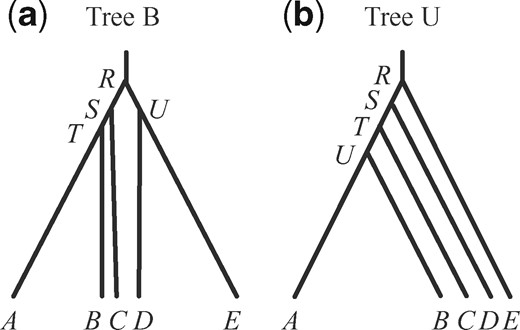
In the first set of simulations, we fix the species tree at either tree B or tree U of figure 1 and estimate the parameters in the MSC model (τs and θs) through Bayesian MCMC. This is analysis A00 in BPP (Yang 2015). Note that both node ages (τs) and population sizes (θs) are measured by genetic distance, in the expected number of mutations per site. We varied the number of loci (L = 40 or 160), the number of sequences per species (S = 2 or 8), and the number of sites in the sequence (N = 250 or 1,000), as well as the mutation rate ( or 0.01). As the species divergence times τs are proportional to θ in our experimental design (fig. 1), the two values of θ mimic different mutation rates. For example, the noncoding and coding parts of the genome have very different neutral mutation rates but may be used to infer the same species divergence history, with nearly proportional parameters (θs and τs) (Shi and Yang 2018; Thawornwattana et al. 2018). The posterior means and 95% highest probability density (HPD) credible intervals (CIs) for the 100 replicate data sets for each simulation setting are shown in figure 2 for tree B. The results for tree U are similar (supplementary fig. S1, Supplementary Material online). The CI width and root-mean-square error (RMSE) calculated using the posterior means as point estimates are in supplementary tables S1 and S2, Supplementary Material online. We are interested in how the information content increases or the estimation precision improves when the amount of data increases in different ways: that is, when the number of loci increases from 40 to 160, the number of sequences per species increases from 2 to 8, or the number of sites in the sequence increases from 250 to 1,000. In each case, the total number of sites (or base pairs) in the data set increases by 4-fold, but the effects on the precision of parameter estimates may differ. Under the MSC model, data at different loci have independent and identical distributions, so that the asymptotic theory may be expected to apply, with the number of loci L to be the sample size. In large data sets (with large L) the posterior CI width and the RMSE may be expected to decrease in proportion to : In other words, a 4-fold increase in L should reduce the RMSE or posterior CI width by a half. Note that the sequence length N cannot be treated as the sample size under the MSC model, because the estimation error will reach a certain nonzero limit when if L is held constant. When the sequences are long so that the gene tree and branch lengths (coalescent times) at each locus are inferred with virtually no errors, adding more sites will add little information but parameter estimates may still involve considerable uncertainties due to coalescent fluctuations among loci.
![(a) Balanced species tree B and (b) unbalanced species tree U for five species, used to simulate data for estimation of parameters in the MSC model (the A00 analysis in Yang [2015]). For tree B, the parameters used are τR = 5θ, τS = 4θ, τT = 3θ, and τU = 4.5θ. For tree U, they are τR = 5θ, τS = 4θ, τT = 3θ, and τU = 2.5θ. Two values of θ are used: 0.0025 and 0.01.](https://oup.silverchair-cdn.com/oup/backfile/Content_public/Journal/mbe/37/11/10.1093_molbev_msaa166/2/m_msaa166f1.jpeg?Expires=1747917497&Signature=ZLuk2Dxxl11TO6XpPHwjaFs6SFGVXbAnp1itL-e9ufzvv9FPptskKybooOEn273CekB-ba4fWQUaEnl0D3U1Fs580NAdCXh3qAsjGuc7ltXepwYzN441-6IOtN2pok8pCwk3HAJbD1GJ~FHMcKo0576apFXPwV8RUecYCZfMZReh2e4w~2-Dkz~PM7N7Fp9FDqjVR8j6MhIt-K71jOllanR2OypnIIJ16E0kS7lvHbxtbfm6MsRb-Uw595texQVyHkPWo1bHWAcmCh~LWl4WXVkdNQSXZ2SNp~TiDRBkOXpwz7wtwmGaURLOL5voHIq3rbczOTC3uPQoyy5aej7LMA__&Key-Pair-Id=APKAIE5G5CRDK6RD3PGA)
(a) Balanced species tree B and (b) unbalanced species tree U for five species, used to simulate data for estimation of parameters in the MSC model (the A00 analysis in Yang [2015]). For tree B, the parameters used are τR = 5θ, τS = 4θ, τT = 3θ, and τU = 4.5θ. For tree U, they are τR = 5θ, τS = 4θ, τT = 3θ, and τU = 2.5θ. Two values of θ are used: 0.0025 and 0.01.
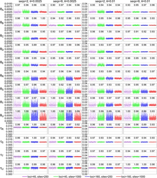
Posterior 95% HPD CIs for the 13 parameters in the MSC model for species tree B (fig. 1) in 100 replicate data sets. The numbers above the CI bars are the CI coverage probability.
Before examining the importance of the various factors, we note that the method or the BPP program behaves as expected. First, with more data and more information, the estimates of all parameters improve and converge to the true values, with the CIs becoming narrower. The CI coverage, or the probability that the 95% HPD CI includes the true parameter value, is in general higher than the nominal 95%, although there were random fluctuations due to limited number of replicates (R = 100) (fig. 2). Note that in our simulation, the parameters are fixed when replicate data sets are generated, so that we are evaluating the frequentist properties of a Bayesian method. In a Bayesian simulation, the parameters would be sampled from their priors for each replicate data set (e.g., Yang and Rannala 2005). There exists no theory to predict that the 95% HPD CI calculated here should include the true value in exactly 95% of the replicate data sets. Nevertheless, Bayesian methods are often found to have good frequentist properties (O’Hagan and Forster 2004). Overall, the results suggest a healthy inference method (fig. 2 and supplementary fig. S1, Supplementary Material online). Second, different parameters are estimated with very different precisions. There are three groups of parameters. In the first group, the population size parameters (θs) for the five modern species (, and E) are well estimated even in moderately sized data sets. In the second group, the θs for the four ancestral species are estimated less well. Among them, θU in tree B is the most poorly estimated (fig. 2 and supplementary fig. S1, Supplementary Material online). Because branch U in tree B is short and deep, few sequences (from D and E) will reach node U and coalesce along the short branch. Note that the probability that all eight sequences from D coalesce in D before reaching U is 0.99988 as the age of node U is coalescent units (fig. 3). Thus, at almost every locus, only two sequences (one from D and one from E) enter U, and they coalesce in branch U with probability 0.632 (fig. 3). Infrequent coalescent events in U lead to poor estimation of θU. This also explains why there is no difference in estimates of θU between S = 2 and 8 (fig. 2). In the third group of parameters, species divergence times (τs) are well estimated in almost all parameter combinations examined. Species trees B and U overall show very similar patterns.
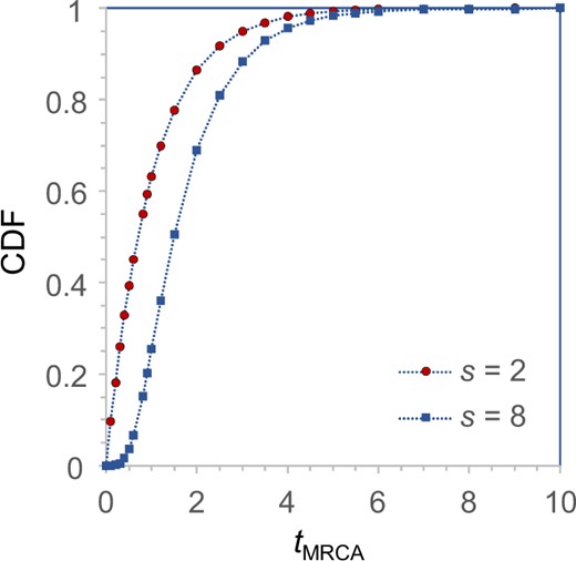
The cumulative distribution function (CDF) for the time to the most recent common ancestor, , for a sample of size s = 2 or 8. Time is measured in the coalescent unit of 2N generations or in the notation of this article. The CDF gives the probability that the whole sample coalesces within the given time. For S = 2, t is exponential with mean 1 and CDF , whereas for S = 8, the CDF is generated by coalescent simulation (with 107 replicates).
Performance improves with the increase in the number of loci (L), the number of sequences per species (S), the number of sites per sequence (N), and the mutation rate (θ). Note that it is meaningful to compare parameter estimates between the two values of θ by using the relative error (i.e., the CI width or RMSE divided by the true value). This mimics the estimation of the effective population size N using genomic regions of different mutation rates, with the expectation that fast evolving loci will be more informative than conserved loci. We start from the least informative data sets with L = 40, S = 2, N = 250, and , and consider the effects of quadrupling the amount of data by increasing the number of loci (L from 40 to 160), the number of sequences (S from 2 to 8), the number of sites (N from 250 to 1,000), and the mutation rate (θ from 0.0025 to 0.01) (fig. 2 and supplementary fig. S1 and tables S1 and S2, Supplementary Material online).
For estimating θs for the five modern species, the most important factor is the number of loci (L), and the least important factors are the number of sites (N) and the mutation rate (θ). For example, the CI width in tree B is in the range 2.19–2.28 in the least informative data sets with S = 2, , N = 250, and L = 40. This is reduced to 1.72–1.82 when longer sequences are used (N = 1,000), to 1.74–1.76 (upon division by 4 to account for the 4-fold difference in the two values of θs) at the higher mutation rate (), to 1.31–1.34 when more sequences are used (S = 8), and to 1.19–1.20 when more loci are used (L = 160). The reduction in the CI width upon quadrupling the number of loci is slightly less than a half (1.19/2.19 = 0.54). The results for species tree U are very similar (supplementary table S2, Supplementary Material online). These results for θs of modern species agree with expectations for estimating θ for one population in the standard coalescent (Felsenstein 2006).
For estimating θs for the four ancestral species, the most important factors are the number of loci (L) and the sequence length (N), whereas the number of sequences (S) is the least important. In the case of tree B and θR, the CI width is 3.23 in the least informative data sets (with S = 2, , N = 250, and ), and this becomes 3.32 (which is even larger) when S = 8, is reduced to 2.51 (after division by 4) when , to 2.47 when L = 160, and to 2.43 when N = 1,000.
For estimating τs, the most important factors are the number of sites (N) and the number of loci (L), which have similar effects, whereas the number of sequences (S) is the least important. For example, in the case of tree B and τR (the age of the root in the species tree), the CI width is 2.69 in the least informative data with S = 2, , N = 250, and L = 40. This becomes 2.66 when S = 8, with virtually no reduction, and is reduced to 1.57 at L = 160, to 1.51 at the higher rate (), and to 1.45 when N = 1,000.
We note that the factors do not always work independently and the effect of one factor may depend on other factors. For example, comparison of the cases L = 40 and N = 1,000 with the case L = 160 and N = 250, other parameters being equal, informs us of the relative importance of L versus N. In the case of tree B, the number of sites (N) is more important than the number of loci (L) for estimating species divergence times (, and τU) at the low mutation rate (), but the two factors have similar effects at the higher mutation rate (with ) (supplementary table S1, Supplementary Material online). In the case of tree U, the two factors have similar effects on estimation of divergence times. As another example, increasing sequence length (N) has a greater effect at the low mutation rate () than at the higher rate (). The reduction in CI width for θA–θE is 17–22% at the lower rate and at the higher rate when S = 2; when S = 8, the reduction is 33% at the lower rate and at the higher rate (supplementary table S1, Supplementary Material online). This may be because at the lower mutation rate, the alignments with N = 250 have few variable sites with little information about the gene tree and coalescent times and increasing sites can effectively improve the information content, whereas at the higher mutation rate (), the alignments with N = 250 sites are already informative and adding more sites will have only minor effects.
Nevertheless, in informative data sets or for estimation of parameters where the asymptotics concerning L is reliable (in other words, when the CI width for L = 40 is about half that for L = 160), the effects of θ, N, and S are noted to be independent of L. For example, the CI-width reduction in θs for the five modern species when N quadruples is 21–23% at L = 40, very close to 22–24% at L = 160. The CI-width reduction in the four τ parameters when N quadruples is 41–46% at , very close to 44–48% at L = 160. Similarly, the effect of mutation rate is similar between L = 40 and L = 160. The CI-width reduction in θA–θE when mutation rate increases by 4-fold is 22–24% and 22–24% at L = 40 and , respectively. The reduction in the CI width for τs is 40–44% at L = 40, very similar to 44–46% at L = 160. Similarly, the effect of the number of sequences (S) is similar between L = 40 and L = 160. The CI-width reduction for θA–θE when S quadruples is 56–57% at 40 and 57% at 160. The CI-width reduction for the τ parameters is only 3–6% at 40 and 2–4% at 160.
We now examine the asymptotic expectation of half reduction in the CI width when the number of loci L increases from 40 to 160. Population size parameters (θs) for modern species are well estimated, and the asymptotics holds well. The reduction in CI width is 46–47% for tree B and 46–49% for tree U in the least informative case (with , S = 2, and N = 250) (supplementary table S1, Supplementary Material online). The reduction is even closer to 50% in the more informative data sets, when , S = 8, and/or N = 1,000. Species divergence times are less well estimated than θs for modern species (in particular τU is poorly estimated) and the asymptotics holds only in the informative data sets. The CI-width reduction in τR, τS, and τT is 31–42% for tree B and 36–44% for tree U in the least informative case (with S = 2, N = 250, and ) and is 49–50% in the most informative case (with S = 8, N = 1,000, and ) for both trees B and U. Ancestral population sizes (θs for R, S, and T) are the most poorly estimated, and the asymptotics is not reliable at such small values of L. The reduction is 23–26% for tree B and 22–30% for tree U in the least informative case (with S = 2, N = 250, and ) and is 47–48% for tree B and 48% for tree U in the most informative case (with S = 8, N = 1,000, and ).
An interesting comparison is between the case of N = 1,000 and and that of N = 250 and , other things being equal. In both cases, the mutation rate for the whole locus is the same. The ratio of CI widths between the two scenarios (with the CI width for divided by 4 to be comparable) is close to 1 (from 0.98 to 1.00) for θs for the five modern species, 0.90–1.00 for θs for the four ancestral species, and 0.92–1.00 for the four species divergence times (τs) (supplementary table S1, Supplementary Material online). Although increasing sites (N) often leads to slightly better performance (in particular, for estimating divergence times) than increasing the mutation rate (θ), the data sets simulated under those two scenarios are nearly equally informative for estimating the parameters in the MSC model.
Species Tree Estimation
In the second set of simulations, we evaluate the power or information content for species tree estimation. We focus on challenging species tree problems with short internal branches (fig. 4). Species tree B has one internal branch of length and two branches of length , whereas species tree U has all three internal branches of length . The probability that two sequences entering the ancestral species will not coalesce in that species is 81.9% for branch length or 67.0% for (fig. 3). Deep coalescence is thus expected to be common in gene trees generated using those species trees.
Species trees B and U for five species () used to simulate data for the A01 analyses. For balanced species tree B, the parameters used are τR = 5θ, τS = 4.8θ, τT = 4.7θ, and τU = 4.8θ. For unbalanced species tree U, we used τR = 5θ, τS = 4.8θ, τT = 4.6θ, and τU = 4.4θ. In each tree, two values of θ are used: 0.0025 and 0.01.
Posterior probabilities for the true species tree in the replicate data sets are shown in figure 5, whereas those for the true subtrees R (which means the whole tree), S, T, and U are listed in table 1. The probability for the true tree increases steadily with the increase in data size and mutation rate and reaches 100% in the most informative data sets of L = 160 loci and N = 1,000 sites at the higher mutation rate () when the true tree is tree U. Tree B is harder to recover than tree U, because of the extremely short branch T, so that the probability for the true tree in the most informative data sets is only 97% (table 1).

Posterior probabilities for the true species tree in 100 replicate data sets for each of the 32 simulation conditions, which are combinations of the species tree (B and U, fig. 4), the number of loci (L = 40 and 160), the number of sequences per species (S = 2 and 8), the number of sites per sequence (N = 250 and 1,000), and the mutation rate ( and 0.01).
Average Posterior Probabilities for the True Subtrees Represented by Nodes R (the whole tree), S, T, and U in Species Trees B and U of Figure 4.
| Data | 2 | 8 | 2 | 8 |
|---|---|---|---|---|
| Tree B | ||||
| L = 40, N = 250 | 0.09, 0.32, 0.46, 0.50 | 0.08, 0.30, 0.39, 0.51 | 0.28, 0.50, 0.60, 0.64 | 0.28, 0.44, 0.56, 0.68 |
| L = 40, N = 1,000 | 0.36, 0.58, 0.65, 0.64 | 0.39, 0.55, 0.66, 0.77 | 0.60, 0.68, 0.71, 0.88 | 0.63, 0.72, 0.74, 0.88 |
| L = 160, N = 250 | 0.40, 0.67, 0.75, 0.66 | 0.39, 0.57, 0.67, 0.75 | 0.78, 0.85, 0.86, 0.92 | 0.81, 0.85, 0.87, 0.95 |
| L = 160, N = 1,000 | 0.90, 0.92, 0.92, 0.98 | 0.90, 0.92, 0.92, 0.98 | 0.92, 0.92, 0.92, 1.00 | 0.97, 0.97, 0.97, 1.00 |
| Tree U | ||||
| L = 40, N = 250 | 0.30, 0.30, 0.46, 0.68 | 0.30, 0.30, 0.46, 0.68 | 0.58, 0.58, 0.73, 0.84 | 0.58, 0.58, 0.72, 0.82 |
| L = 40, N = 1,000 | 0.70, 0.70, 0.85, 0.91 | 0.68, 0.68, 0.84, 0.88 | 0.87, 0.87, 0.94, 0.96 | 0.93, 0.93, 0.95, 0.97 |
| L = 160, N = 250 | 0.74, 0.74, 0.93, 0.95 | 0.76, 0.76, 0.93, 0.95 | 0.97, 0.97, 0.99, 1.00 | 0.97, 0.97, 0.99, 1.00 |
| L = 160, N = 1,000 | 0.99, 0.99, 1.00, 1.00 | 0.99, 0.99, 1.00, 1.00 | 1.00, 1.00, 1.00, 1.00 | 1.00, 1.00, 1.00, 1.00 |
Note.—Averages are over the 100 replicate data sets. Probabilities for R are plotted in figure 5.
The Bayesian estimate of the species tree is the one with the maximum posterior probability (or the MAP tree, Rannala and Yang 1996). The probabilities that the MAP tree includes the true subtrees increase steadily with the increase in the amount of data (table 2). The 95% credible set tends to include the true species tree with probabilities higher than the nominal 95% (table 3). When the amount of data increases, the CI size decreases, eventually with only one tree (the true tree) in the credible set. These results indicate good performance of Bayesian estimation of the species tree, consistent with previous simulation studies (Ogilvie et al. 2016; Rannala and Yang 2017).
Proportions of Simulated Replicates in Which the MAP Tree Includes the True Subtrees R, S, T, and U in Species Trees B and U of Figure 4.
| Data | 2 | 8 | 2 | 8 |
|---|---|---|---|---|
| Tree B | ||||
| L = 40, N = 250 | 0.11, 0.43, 0.57, 0.47 | 0.03, 0.34, 0.42, 0.43 | 0.40, 0.61, 0.71, 0.71 | 0.46, 0.61, 0.65, 0.74 |
| L = 40, N = 1,000 | 0.55, 0.74, 0.80, 0.76 | 0.60, 0.75, 0.80, 0.84 | 0.77, 0.82, 0.82, 0.93 | 0.77, 0.83, 0.83, 0.91 |
| L = 160, N = 250 | 0.65, 0.85, 0.90, 0.76 | 0.60, 0.74, 0.80, 0.81 | 0.86, 0.91, 0.91, 0.94 | 0.96, 0.97, 0.97, 0.99 |
| L = 160, N = 1,000 | 0.99, 0.99, 0.99, 1.00 | 0.97, 0.97, 0.97, 1.00 | 0.96, 0.96, 0.96, 1.00 | 0.99, 0.99, 0.99, 1.00 |
| Tree U | ||||
| L = 40, N = 250 | 0.52, 0.52, 0.68, 0.79 | 0.50, 0.50, 0.66, 0.80 | 0.82, 0.82, 0.92, 0.95 | 0.77, 0.77, 0.87, 0.89 |
| L = 40, N = 1,000 | 0.92, 0.92, 0.96, 0.96 | 0.85, 0.85, 0.97, 0.97 | 0.98, 0.98, 1.00, 1.00 | 1.00, 1.00, 1.00, 1.00 |
| L = 160, N = 250 | 0.89, 0.89, 1.00, 1.00 | 0.91, 0.91, 0.99, 1.00 | 0.99, 0.99, 1.00, 1.00 | 1.00, 1.00, 1.00, 1.00 |
| L = 160, N = 1,000 | 1.00, 1.00, 1.00, 1.00 | 1.00, 1.00, 1.00, 1.00 | 1.00, 1.00, 1.00, 1.00 | 1.00, 1.00, 1.00, 1.00 |
Average Size (the average number of species trees) and Coverage of the 95% Credible Set of Species Trees in Data Simulated Using Species Trees B and U of Figure 4.
| Data | 2 | 8 | 2 | 8 |
|---|---|---|---|---|
| Tree B | ||||
| L = 40, N = 250 | 15.9, 0.90 | 13.7, 0.86 | 9.26, 0.96 | 10.1, 0.99 |
| L = 40, N = 1,000 | 7.40, 0.97 | 7.00, 0.97 | 3.66, 0.96 | 3.34, 1.00 |
| L = 160, N = 250 | 6.46, 0.97 | 7.07, 0.98 | 2.32, 0.99 | 2.31, 1.00 |
| L = 160, N = 1,000 | 1.75, 1.00 | 1.66, 1.00 | 1.41, 1.00 | 1.19, 1.00 |
| Tree U | ||||
| L = 40, N = 250 | 14.8, 0.96 | 15.1, 0.98 | 4.99, 1.00 | 4.67, 1.00 |
| L = 40, N = 1,000 | 3.73, 1.00 | 3.51, 1.00 | 1.84, 1.00 | 1.63, 1.00 |
| L = 160, N = 250 | 2.61, 1.00 | 2.48, 1.00 | 1.15, 1.00 | 1.16, 1.00 |
| L = 160, N = 1,000 | 1.09, 1.00 | 1.08, 1.00 | 1.00, 1.00 | 1.00, 1.00 |
To evaluate the information content in the data sets, we use the average posterior probability for the true species tree (fig. 5 and table 1). Using the probability that the MAP tree is the true species tree (table 2) leads to the same conclusions. The number of loci (L) is the most important factor for improving the power of inference, followed the number of sites (N) and the mutation rate (θ), whereas the number of sequences per species (S) is the least important. For example, the probability for the true species tree is only 9% when the true species tree is tree B in the least informative data (with S = 2, , N = 250, and L = 40). This probability stays almost unchanged (8%) when more sequences are used (S = 8) and rises to 28% at the higher mutation rate (), to 36% when longer sequences are used (N = 1,000), and to 40% when more loci are used (L = 160). The same pattern holds if we consider the probabilities for the true subtrees (S, T, and U) or if the true species tree is tree U (table 1). For some parameter settings (e.g., tree U, , N = 1,000, and L = 40), the probability is even lower at S = 8 than at S = 2 (table 1), but the differences are small and may be attributed to random errors.
We now compare the error rates in species tree estimation between the case of N = 1,000 and with that of N = 250 and , other things being equal. Although the locus-wide mutation rates are the same, a longer sequence with a lower mutation rate (N = 1,000 and ) gives a better performance than a shorter sequence with a higher mutation rate (N = 250 and ). For example, when and S = 2, the average posterior for the correct species tree is 0.36 at N = 1,000 and , in comparison with 0.28 at N = 250 and for tree B (table 1). The same conclusion holds for other combinations of L and S and for tree U. Similarly, quadrupling the sequence length (N) leads to higher probabilities that the estimated species tree is correct and to greater reductions in the credible set than quadrupling the mutation rate (θ). The larger effects of N than θ on species tree estimation are somewhat surprising, especially as the two factors have nearly equal importance for parameter estimation under the MSC, as discussed earlier.
Species Delimitation
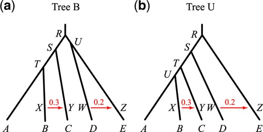
In the third set of simulations, we evaluate the information content for delimiting species using the approach of Bayesian model selection (Yang and Rannala 2010). Our simulation model assumes five populations (A, B, C, D, and E) and three species (AB, C, and DE) with the phylogeny (fig. 6). We used two sets of parameters representing two tree shapes. With tree shape 1 ( and ), the species phylogeny is challenging because of the short internal branch. With tree shape 2 ( and ), species delimitation is challenging because the species divergence times are similar to the average coalescent times so that the between-species divergence is not much greater than the within-species polymorphism (fig. 6).
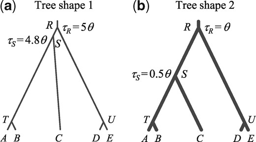
The true species trees or MSC models used in the simulation for species delimitation. There are five populations (, and E) and three species (AB, C, and DE) in the true model. Data are simulated by assuming the tree of five populations with τT and τU set to very small values (), and then analyzed to infer both the species delimitation and species phylogeny (the A11 analysis, Yang 2015). Two sets of parameters are used to represent different tree shapes: (a) and and (b) and . The thickness of the branches indicates the population sizes (θs) relative to the species divergence times (τs). Two values are used for θ: 0.0025 or 0.01.
For tree shape 1 (fig. 6a), the probabilities of recovering the correct delimitation or correct delimited species (AB, C, and DE) grow rapidly when the amount of data increases, but the probability of recovering the whole model (the correct delimitation and correct species phylogeny) remains far away from 100% except for the most informative data sets with , and (fig. 7 and tables 4 and5). Because of the short internal branch in the true species tree, the species phylogeny is hard to recover even when the species are correctly delimited. Furthermore, species C is easier to delimit or identify than species AB and DE as it is farther away from other species.
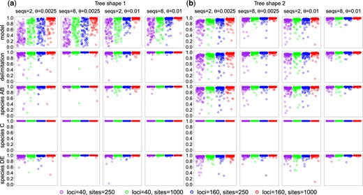
Posterior probability of the correct model (both delimitation and phylogeny), correct delimitation, and correct delimited species AB, C, and DE in the A11 analysis of joint species delimitation and species tree estimation (Yang 2015). Two sets of model parameters are used for the model of figure 6: (a) and (b) and .
Average Posterior Probabilities for the True Model, True Delimitation, and True Species AB, C, and DE for the Model of Figure 6.
| 2 | 8 | 2 | 8 | |
|---|---|---|---|---|
| Tree shape 1 | ||||
| L = 40, N = 250 | 0.42, 0.90, 0.95, 1.00, 0.96 | 0.46, 0.99, 0.99, 1.00, 0.99 | 0.66, 0.95, 0.98, 1.00, 0.97 | 0.66, 0.99, 0.99, 1.00, 1.00 |
| L = 40, N = 1,000 | 0.63, 0.94, 0.96, 1.00, 0.97 | 0.63, 0.98, 0.99, 1.00, 1.00 | 0.77, 0.97, 0.98, 1.00, 0.99 | 0.81, 1.00, 1.00, 1.00, 1.00 |
| L = 160, N = 250 | 0.63, 0.95, 0.97, 1.00, 0.98 | 0.64, 1.00, 1.00, 1.00, 1.00 | 0.90, 0.98, 0.99, 1.00, 0.99 | 0.90, 1.00, 1.00, 1.00, 1.00 |
| L = 160, N = 1,000 | 0.86, 0.97, 0.99, 1.00, 0.98 | 0.88, 0.99, 0.99, 1.00, 1.00 | 0.98, 0.98, 0.99, 1.00, 1.00 | 0.99, 1.00, 1.00, 1.00, 1.00 |
| Tree shape 2 | ||||
| L = 40, N = 250 | 0.74, 0.74, 0.81, 1.00, 0.91 | 0.92, 0.92, 0.94, 1.00, 0.98 | 0.83, 0.83, 0.88, 1.00, 0.95 | 0.96, 0.96, 0.97, 1.00, 0.99 |
| L = 40, N = 1,000 | 0.85, 0.85, 0.90, 1.00, 0.95 | 0.96, 0.96, 0.98, 1.00, 0.99 | 0.89, 0.89, 0.93, 1.00, 0.96 | 0.97, 0.97, 0.98, 1.00, 0.99 |
| L = 160, N = 250 | 0.84, 0.84, 0.89, 1.00, 0.95 | 0.96, 0.96, 0.98, 1.00, 0.98 | 0.90, 0.90, 0.93, 1.00, 0.97 | 0.98, 0.98, 0.99, 1.00, 0.99 |
| L = 160, N = 1,000 | 0.91, 0.91, 0.93, 1.00, 0.97 | 0.98, 0.98, 0.99, 1.00, 0.99 | 0.95, 0.95, 0.97, 1.00, 0.97 | 0.99, 0.99, 0.99, 1.00, 1.00 |
Note.—The five numbers in each cell are for the true model, true delimitation, and the three true delimited species (AB, C, and DE). The true model means that the number of species is 3, the three species are AB, C, and DE, and the phylogeny is . The true delimitation means that the number of species is 3 and the three species are AB, C, and DE but the phylogeny may and may not be correct.
Proportions of Replicates in Which the MAP Model Is the True Model, and Includes the True Delimitation, and True Species AB, C, and DE for the Models of Figure 6.
| 2 | 8 | 2 | 8 | |
|---|---|---|---|---|
| Tree shape 1 | ||||
| L = 40, N = 250 | 0.50, 0.97, 0.97, 1.00, 1.00 | 0.56, 1.00, 1.00, 1.00, 1.00 | 0.79, 0.99, 1.00, 1.00, 0.99 | 0.80, 1.00, 1.00, 1.00, 1.00 |
| L = 40, N = 1,000 | 0.74, 0.97, 0.98, 1.00, 0.99 | 0.76, 0.99, 0.99, 1.00, 1.00 | 0.87, 1.00, 1.00, 1.00, 1.00 | 0.91, 1.00, 1.00, 1.00, 1.00 |
| L = 160, N = 250 | 0.78, 0.99, 0.99, 1.00, 1.00 | 0.75, 1.00, 1.00, 1.00, 1.00 | 1.00, 1.00, 1.00, 1.00, 1.00 | 0.97, 1.00, 1.00, 1.00, 1.00 |
| L = 160, N = 1,000 | 0.94, 0.98, 0.99, 1.00, 0.99 | 0.98, 1.00, 1.00, 1.00, 1.00 | 1.00, 1.00, 1.00, 1.00, 1.00 | 1.00, 1.00, 1.00, 1.00, 1.00 |
| Tree shape 2 | ||||
| L = 40, N = 250 | 0.90, 0.90, 0.93, 1.00, 0.97 | 0.98, 0.98, 0.98, 1.00, 1.00 | 0.94, 0.94, 0.95, 1.00, 0.99 | 1.00, 1.00, 1.00, 1.00, 1.00 |
| L = 40, N = 1,000 | 0.97, 0.97, 0.97, 1.00, 1.00 | 1.00, 1.00, 1.00, 1.00, 1.00 | 0.97, 0.97, 0.98, 1.00, 0.99 | 1.00, 1.00, 1.00, 1.00, 1.00 |
| L = 160, N = 250 | 0.94, 0.94, 0.96, 1.00, 0.98 | 0.99, 0.99, 1.00, 1.00, 0.99 | 0.97, 0.97, 0.97, 1.00, 1.00 | 1.00, 1.00, 1.00, 1.00, 1.00 |
| L = 160, N = 1,000 | 0.99, 0.99, 0.99, 1.00, 1.00 | 1.00, 1.00, 1.00, 1.00, 1.00 | 0.99, 0.99, 1.00, 1.00, 0.99 | 1.00, 1.00, 1.00, 1.00, 1.00 |
For recovering the whole model (fig. 6a), the importance of the factors is in the order of mutation rate (θ), the number of loci (L), and the number of sites (N), and then the number of sequences (S). For example, the average posterior probability for the true model is 0.42 in the least informative data sets (with , L = 4, N = 250, and S = 2). This rises to 0.46 when S = 8, to 0.63 when N = 1,000 or L = 160, and to 0.66 at the high mutation rate () (table 4). If we disregard the phylogeny and focus on delimitation only, the most important factor is the number of sequences (S), followed by the mutation rate (θ), and then by the number of loci (L) and the number of sites (N). For example, the average posterior probability for the true delimitation is 0.90 in the least informative data sets (with , L = 4, N = 250, and S = 2), and this rises to 0.94 when N = 1,000, to 0.95 when , to 0.95 when L = 160, and to 0.99 when S = 8 (table 4). The importance of the number of sequences to species delimitation contrasts with species tree estimation, in which the number of sequences is the least important factor among those examined here. The pattern is the same if we use the probabilities that the MAP model is the true model or includes the true delimitation.
For tree shape 2 (fig. 6b), the phylogeny is easy to reconstruct because of the long internal branch, and the correct species tree is always recovered if the delimitation is correct. As a result, the probability for the correct model is the same as that for the correct delimitation. The number of sequences S is the most important for the inference, whereas the other factors (L, N, and θ) are of equal importance. For example, the average posterior probability for the true model and true delimitation is 0.74 in the least informative data sets (with , L = 40, N = 250, and S = 2). This rises to 0.92 when S = 8, compared with 0.85 for N = 1,000, 0.84 for , and 0.83 for (table 4). If we focus on species delimitation, the number of sequences is the most influential for both trees of figure 6.
Estimation of Introgression Parameters under the MSci Model
In the fourth set of simulations, we examine the estimation of parameters under the MSci model, in particular, the introgression probability parameters (fig. 8). We use two models or trees, each with 21 parameters (fig. 8). As in the A00 simulation under the MSC model without gene flow, the θs for the five extant species are all well estimated, as are the six divergence times (τs). However, θs for the eight ancestral species are more poorly estimated. Among them, θU in tree B has substantial uncertainties even in the most informative data sets (supplementary fig. S2 and tables S3 and S4, Supplementary Material online).
Two introgression (MSci) models used in the simulation. The parameters for tree B are τR = 5θ, τS = 4θ, τT = 3θ, τU = 4.5θ, , and , whereas those for tree U are τR = 5θ, τS = 4θ, τT = 3θ, τU = 2.5θ, , and . In both trees, we have and and use two values for θ: 0.0025 or 0.01.
The relative importance of the various factors to the estimation precision is similar to what was found earlier for the MSC simulation. For estimation of θs for the modern species, the number of sites (N) is the least important, followed by the mutation rate (θ) and the number of sequences (S), whereas the number of loci (L) is the most influential. For estimation of θs for the ancestral species, the number of sequences (S) is the least important, followed by the mutation rate (θ), and the number of loci (L), whereas the number of sites (N) is the most influential. For estimation of species divergence times (e.g., τR), the number of sequences (S) is the least important, followed by the mutation rate (θ) and the number of loci (L), whereas the number of sites (N) is the most influential.
The reduction in the CI width upon quadrupling the number of loci (L) is 46–50% for θs for modern species, only 6–24% for θs for the ancestral species, and 33–53% for the species divergence times (τs) in the least informative case. As before, the reduction is close to a half when the parameters are well estimated and the asymptotics is reliable but less than a half for poorly estimated parameters.
Here, we focus on the estimation of the introgression probabilities ( and ) (fig. 9 and supplementary tables S3 and S4, Supplementary Material online). The least important factor is the number of sequences (S), whereas the most important factor is the number of loci (L). For example, the CI width for in model tree B is 0.343 in the least informative data sets (with S = 2, , N = 250, and L = 40). This is reduced to 0.303 when the number of sequences is increased to S = 8, to 0.272 at , to 0.264 at N = 1,000, and to 0.178 at L = 160. The reduction in the CI width upon quadrupling the number of loci is 48%, close to a half. For introgression parameter , the mutation rate is more important than the number of sites, but again the number of sequences (S) is the least important, whereas the number of loci (L) is the most influential. The results are similar for the MSci model U (fig. 9 and supplementary tables S3 and S4, Supplementary Material online).
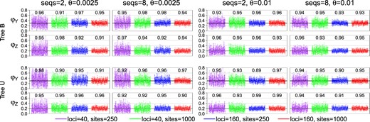
Posterior 95% CIs and CI coverage in 100 replicate data sets for introgression parameters in the MSci model of figure 8. The numbers above or below the CI bars are the CI coverage probability. Results for all 21 parameters in the model are shown in supplementary figures S2 and S3, Supplementary Material online.
Discussion
Measures of Performance
The performance of phylogenetic tree reconstruction is often measured using the Robinson–Foulds distance (Robinson and Foulds 1981) between the inferred tree and the true tree. Sometimes, a modified measure is used that incorporates the branch lengths in the true and estimated trees, with the rationale that an incorrectly inferred clade with a short branch is less serious than one with a long branch (Kuhner and Felsenstein 1994). The measure of Ogilvie et al. (2016) uses averages over the whole posterior distribution, so that it incorporates both errors of model selection (errors in tree topology) and of parameter estimation (errors in branch lengths), as well as the calculated measure of confidence in the point estimate (posterior probability). Because the asymptotics are very different for errors in model selection and in parameter estimation, we have in this article separated the two inference problems in our measure to simplify the interpretation of the simulation results. We used standard measures of performance in statistics, such as the probability of incorrectly selected model and the width of the CI or RMSE for parameter estimation. Parameter estimation is considered only if the model is fixed or if the inferred model is correct, as parameters in incorrectly inferred models may not have meaningful biological interpretations.
Information Content in Phylogenomic Data Sets
This study deals with the question of what kinds of multilocus sequence data sets are most informative for addressing inference problems under the MSC model, such as estimation of evolutionary parameters, estimation of species trees, and delimitation of species. The study is in the realm of experimental design and aims to provide useful insights into the best sequencing strategy concerning the nature of genomic regions targeted (such as the mutation rate), the number of loci (or genomic regions), the number of samples per species, etc. given the focus of the study. Table 6 provides a brief summary of our findings. Here, we note a number of limitations of our study, which may affect the interpretations of our results.
Relative Importance of the Different Factors Examined in This Article (the number of loci L, the number of sequences per species per locus S, the sequence length N, and the mutation rate θ) to Different Inference Problems under the MSC.
| Analysis | Influencea | N versus θb |
|---|---|---|
| Parameter estimation under MSC and MSci (A00) | ||
| θs for modern species | ||
| θs for ancestral species | ||
| τs | ||
| s | ||
| Species tree estimation under MSC (A01) | ||
| Analysis | Influencea | N versus θb |
|---|---|---|
| Parameter estimation under MSC and MSci (A00) | ||
| θs for modern species | ||
| θs for ancestral species | ||
| τs | ||
| s | ||
| Species tree estimation under MSC (A01) | ||
means that increasing the number of loci (L) improves information content more than increasing the number of sequences (S), which is in turn more effective than increasing the sequence length (N) or the mutation rate (θ), while N and θ have similar effect.
means that when the locus-wide mutation rate () is fixed, a longer sequence with a lower mutation rate gives better performance than a shorter sequence with a higher mutation rate, whereas means that the two have similar performance.
First, we have examined only two levels for each of the factors considered and have explored only a very small portion of the parameter space, due to computational costs. It may not be safe to generalize to regions of the parameter space not examined in our simulation. The information content is a complex function of the values of parameters in the MSC model and the factors we considered (the number of loci L, the number of sequences per species S, and the number of sites per sequence N), and the multiple factors may be interdependent. An ideal situation for using simulation may be where a body of theory exists to predict the method behavior and simulation is then used to confirm the theory and delineate its limits of applicability. In this regard, the large-sample asymptotics applies with the increase in the number of loci L, as confirmed in our simulation: Quadrupling the number of loci reduces the CI width by a half for parameters that are well estimated (or if L is sufficiently large). However, we lack similar theories concerning S and N. A practical problem is to identify the point of diminished returns. For example, two sequences are clearly more informative than one sequence (some parameters are unidentifiable when only one sequence is sampled from each species) and we expect performance to increase quickly initially when we add more sequences to the data set but beyond a certain number, including more sequences will add very little extra information. For species tree estimation, it seems that going beyond two sequences may not be important.
Second, our simulation ignored many issues such as the challenges and costs of sampling and sequencing (Edwards et al. 2017; Karin et al. 2020), and the issues of coverage and sequencing errors (Lemmon and Lemmon 2013). Advancements in sequencing technologies and reduction of sequencing cost mean that such factors may be more important than information for inference in evolutionary biology when sequencing priorities are determined. Sometimes genomes are sequenced as a valuable primary source of data that can be utilized in a variety of ways in the future. Nevertheless, inference content in the resulting data sets should be an important factor to consider. Another use of results on information content is to advise on data subsampling. Analysis of genomic sequence data using full-likelihood inference methods is computationally expensive, and it is often necessary to subsample existing data to make the computation feasible. The results of this study may then be useful for establishing good practices of data subsampling. For example, for species tree estimation, it is far better to include many loci or genomic regions than many samples from the same species.
Third, we have assumed the molecular clock and the JC mutation model in the simulation and analysis of the data, and our study concerns coalescent-based inference for closely related species only, at low sequence divergences (say, within 10%). The coalescence process affects deep phylogenies as well, since the issue lies with the length rather than the depth of the internal branches on the phylogeny (Edwards et al. 2005). However, inference of deep phylogenies incorporating the coalescent process and relaxed clocks involves many challenges, which are beyond the scope of our study (Xu and Yang 2016).
Finally, we have used the program BPP as a representative of full-likelihood methods and our results may not apply to methods based on summary statistics. Summary methods have a huge computational advantage and may be the only methods feasible in analysis of very large data sets. For species tree estimation, ASTRAL and MP-EST (Liu et al. 2010) infer gene trees at individual loci, and then construct a species tree estimate treating the gene trees as given data. In such a two-step approach, the reliability of the inferred gene trees may affect the performance, so that the number of sites may be important (Mossel and Roch 2017). For full-likelihood methods, phylogenetic errors are not a major concern (Liu et al. 2015; Xu and Yang 2016), although increasing sequence length increases information content as well. For parameter estimation, full-likelihood methods may be necessary, because summary methods such as ASTRAL and MP-EST can estimate the internal branch lengths in coalescent units on the species tree but cannot identify or estimate most parameters in the MSC or MSci models (Xu and Yang 2016; Zhu and Degnan 2017; Flouri et al. 2020). We leave it to future studies to examine the relative importance of various factors to performance of summary methods.
Computational Issues
In this article, we examined the statistical performance of BPP under the MSC model (either with or without cross-species introgression) but ignored the computational requirements and mixing issues of MCMC algorithms. Computational will be an important factor when one subsamples data to apply full-likelihood methods of inference. Computation increases with the increase in the number of species/populations, the number of loci, the number of sequences per locus, and the number of sites per sequence. The number of species may have the greatest impact, because more species mean many more species trees and a much expanded parameter space. The number of sites should be the least important factor that affects computation. Although there are more site patterns under complex models such as GTR (Yang 1994) than under JC, computation is proportional to the number of site patterns and grows sublinearly with the number of sites under any model. In comparison, computation grows much faster with the increase in the number of species, the number of sequences, and the number of loci. The increased computational effort may manifest itself in two ways. First, with more data, each iteration of the MCMC algorithm takes more computation, mainly because the phylogenetic likelihood (the probability of observing the sequence alignment at the locus given the gene tree and coalescent times) is more expensive. In typical data analysis, the likelihood calculation accounts for most (>80%) of the CPU time. The likelihood calculation on a gene tree grows roughly linearly with the number of sequences, although more sequences at each locus also mean more gene trees and branch lengths to average over. Second, with more data, the posterior distribution of the parameters (θs and τs) under each species tree becomes more concentrated. As a result, it becomes more difficult to move from one species tree to another in the trans-model MCMC algorithm, and many more iterations will be necessary to allow adequate sampling of the posterior (Yang 2014, pp. 254–255). If the proposed parameter values for the new species tree are poor and far away from the posterior mode, which is very likely when the within-model parameter posterior is spiky, the proposal will most likely be rejected even if the new species tree has a higher posterior than the current species tree. In large data sets, the problem of poor mixing appears to be a far greater challenge than the problem of more expensive likelihood calculation per MCMC iteration (Rannala and Yang 2017).
Materials and Methods
A00 Estimation of Divergence Times and Population Size Parameters
The first set of simulations examined the estimation of parameters in the MSC model (θs and τs), with the species tree fixed. Data were generated using the “simulate” option of BPP (Yang 2015; Flouri et al. 2018). Gene trees with branch lengths (coalescent times) were simulated under the MSC model (Rannala and Yang 2003). Then, sequences were “evolved” along the branches of the gene tree according to the JC model (Jukes and Cantor 1969), and the sequences at the tips of the gene tree constituted the data at the locus. We assumed species trees B or U of figure 1. For tree B, the parameters were τR = 5θ, τS = 4θ, τT = 3θ, and τU = 4.5θ, with two values for θ: 0.0025 and 0.01. For tree U, we used τR = 5θ, τS = 4θ, τT = 3θ, and τU = 2.5θ, with 0.0025 or 0.01. We sampled either S = 2 or 8 sequences per species at each locus, with the sequence length to be either N = 250 or 1,000 sites. The number of loci was either 40 or 160. Each replicate data set consisted of L loci, with 10 or 40 sequences per locus. The number of replicate data sets was 100. The total number of simulated data sets, for all the combinations of tree, S, N, L, and θ is thus .
Each replicate data set was analyzed using BPP version 4 (Flouri et al. 2018) to estimate the parameters in the MSC model (τs and θs on the species tree). The correct species tree and the correct model (JC) were assumed. Inverse-gamma priors were assigned on the population size parameters (θ) and the age of the root on the species tree (), with the shape parameter 3 and the prior means equal to the true values: IG(3, 0.025) and IG(3, 0.005) for , and IG(3, 0.1) and IG(3, 0.02) for . The inverse-gamma distribution with shape parameter α = 3 has the coefficient of variation 1 and constitutes a diffuse prior. Note that although the same θ for all species on the species tree was assumed in the simulation, every branch on the species tree had its own θ when the data were analyzed using BPP.
Pilot runs were used to determine the suitable settings for the MCMC, and then the same setting was used to analyze all replicates. Convergence was assessed by running the same analysis multiple times and confirming consistency between runs (Yang 2015; Flouri et al. 2018). We used 32,000 iterations for burnin, after which we took 105 samples, sampling every five iterations. Analysis of each data set took ≈4 h on a single core for small data sets of 40 loci and ten sequences per locus or ≈23 h for large data sets of 160 loci and 40 sequences per locus.
A01 Species Tree Estimation
The second set of simulations examined the estimation of the species tree topology under the MSC model. Multilocus sequence data were simulated assuming species trees B or U of figure 4. For tree B, the parameters were , and . For tree U, they were , and . Two values were used for θ: 0.0025 and 0.01. The other parameters and data configurations were the same as in the A00 simulation. In total, 3,200 replicate data sets were simulated.
Each data set was analyzed using BPP to estimate the species tree. The subtree-pruning-and-regrafting algorithm was used to move between species trees (Rannala and Yang 2017; Flouri et al. 2018). During the pilot runs, the program showed mixing problems in some large data sets (with S = 8 sequences and L = 160 loci). It was found helpful to integrate out θs analytically through the use of the conjugate inverse-gamma priors (Flouri et al. 2018). Furthermore, the starting species tree was noted to affect the time taken to reach stationarity or the specification of the burnin, but not the mixing efficiency of the Markov chain after the burnin. Thus, we used the true species tree as the starting tree. We calculated the posterior probabilities for the species tree and clades to measure performance.
A11 Species Delimitation
The third set of simulations examined species delimitation using multilocus data sets under the MSC model (Yang and Rannala 2010, 2014). There are three species (AB, C, and DE) and five populations (, and E) in the true model (fig. 6). Two sets of node ages are used to represent different tree shapes: 1) and (fig. 6a) and 2) (fig. 6b). We simulated gene trees and sequence alignments by using the true species tree for five populations with τT and τU close to 0. The number of sequences for each of the five populations was either 2 or 8. Other parameter settings were as before. A total of 3,200 data sets were simulated.
Each replicate data set was analyzed to infer both the species delimitation and species phylogeny (analysis A11 in Yang [2015]). Five populations, with the correct assignment of sequences to populations, were assumed in the analysis, and the program evaluates different models of merging the five populations into species as well as different species phylogenies (if the number of delimited species is 3 or more) (Yang and Rannala 2014). Trans-dimensional reversible-jump MCMC (Yang and Rannala 2010; Rannala and Yang 2013) was used to move between different delimitation models, whereas the subtree-pruning-and-regrafting algorithm (Yang and Rannala 2014; Rannala and Yang 2017) was used to move between species trees. Similarly, θs were integrated out analytically through the use of inverse-gamma priors to improve mixing (Flouri et al. 2018). The starting model was generated by collapsing at random some of the four internal nodes on the five-population tree (fig. 6) (Yang and Rannala 2010). Posterior probabilities for inferring the correct model or correct delimitation were calculated.
A00-MSci Estimation of Introgression Parameters under the MSci Model
The fourth set of simulation explored the performance of BPP under the two MSci models of figure 8 (Flouri et al. 2020). In each model, there were two unidirectional introgression events. The parameters for tree B were , , and . Parameters for tree U were , and . In both trees, and . Two values were used for θ: 0.0025 or 0.01. Gene trees and sequence alignments were simulated using BPP under the JC model. A total of 3,200 replicate data sets were generated. Each data set was then analyzed to estimate the 21 parameters in the MSci model (Flouri et al. 2020).
Supplementary Material
Supplementary data are available at Molecular Biology and Evolution online.
Acknowledgments
We thank two anonymous reviewers for comments. This study has been supported by Biotechnology and Biological Sciences Research Council (Grant No. BB/P006493/1 to Z.Y.) and a BBSRC Equipment Grant (BB/R01356X/1). J.H.’s visit to London was supported by China Scholarship Council (CSC).
