Prospects for Building Large Timetrees Using Molecular Data with Incomplete Gene Coverage among Species Free

Introduction

Estimating species divergence times is important to understanding the history of life. Because of the ease of sequence data acquisition and our ability to statistically model the evolutionary patterns of change, molecular sequences have become most widely used for this purpose (Kumar and Hedges 1998; Cracraft and Donoghue 2004; Kumar 2005; Douzery et al. 2006). Several programs and methods have been developed using varying underlying models of evolution (including patterns of evolutionary rate variation) to analyze such data sets, which have been applied to all major groups of organisms (Sanderson 1997; Rambaut and Bromham 1998; Kishino et al. 2001; Sanderson 2002; Thorne and Kishino 2002; Rutschmann 2006; Drummond and Rambaut 2007; Hedges and Kumar 2009; Battistuzzi et al. 2010; Brown and Yang 2011; Tamura et al. 2012). Most molecular sequence data sets available for building timetrees are rapidly growing in terms of both genes and species represented. However, they are frequently sparse; that is, the sequences from orthologous genes and genomic segments are not available for all the species included (Yoder and Yang 2004; Sanderson et al. 2010). This is primarily due to sampling bias but also may be caused by gene loss and gain in some lineages. We refer to such data sets as having incomplete coverage.

Interestingly, systematic assessment of the impact of missing data on divergence time estimation remains to be studied, even though the effects of such missing data on the accuracy of inference of evolutionary tree topology and branch lengths have been extensively studied for over a decade with mixed results (Philippe et al. 2004; Lemmon et al. 2009; Wiens and Morrill 2011; Wiens et al. 2012; Roure et al. 2013). If the negative effects of missing data on divergence time estimation are substantial, then it would be necessary to devise criteria to select subsets of species and genes for inclusion in the data set so as to reduce data sparseness (fraction of missing data in the gene-by-species matrix) and achieve higher accuracy of time estimation. In contrast, if the accuracy of time estimates is not adversely affected by the missing data for many genes in different species, then the prospects of building very large trees encompassing thousands of species, even those that have not been extensively sequenced.

Therefore, we conducted computer simulations to estimate the change in the accuracy of divergence time estimates produced by the RelTime method (Tamura et al. 2012) when the sequence data set becomes progressively smaller, either because of sparseness of the data matrix or the availability of fewer numbers of genes. This was done for simulated data sets that contain genes exhibiting extensive evolutionary rate differences among lineages (randomly varying rates [RRs] as well as autocorrelated rates [ARs]). We have augmented these analyses by using an empirical sequence data set to evaluate the applicability of simulation results to real data sets. Our results point to brighter prospects for inferring large timetrees than intuitively anticipated, as even extremely sparse data sets containing many genes often allowed robust divergence time estimation.

Results

We assessed the absolute and comparative accuracy of divergence time estimates by means of computer-simulated alignments that contained data from a realistic binary phylogenetic tree of 446 taxa (Tamura et al. 2012). Here, substitution parameters obtained from a natural sequence set were used. We considered three evolutionary rate scenarios: Constant rate (CR) among lineages, stochastically varying ARs among lineages, and uncorrelated RR. (See fig. 1 and Materials and Methods for more details.) The resulting alignments (CR, AR, and RR) were analyzed using the RelTime software (Tamura et al. 2012), which can rapidly infer timetrees for data sets containing hundreds of species when compared with other approaches (Thorne and Kishino 2002; Drummond and Rambaut 2007) requiring prohibitively large computational time (Tamura et al. 2012). When multiple genes were used, sequences from the genes were concatenated together into a supergene and subjected to RelTime analysis.

Fig. 1.

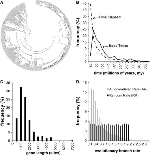
Model tree and substitution patterns. (A) A 446-taxa phylogeny used for computer simulations. (B) Distribution of node divergence times (solid line) in the tree. The dashed line represents the distribution of elapsed time along branches of the tree. (C) Distribution of simulated gene alignment length, based on empirically observed gene lengths. (D) Rates were varied in the simulations to span a variety of models and evolutionary patterns. Because we generally do not have knowledge of actual rate variation patterns in real situations, we used three types of simulated evolutionary rate variation: As a baseline, a CR scenario, one in which the rate variation among branches was autocorrelated (AR), and one in which the (expected) evolutionary rates varied independently on each branch based on a uniform distribution, as described in Materials and Methods. A histogram is shown of the distribution of simulated rates in each case, with the nominal rate set equal to 1.0. In the CR case, the length distribution would be represented by a single bin at x = 1.0.

Open in new tabDownload slide

As the initial benchmark, we considered the simplest situation, where we had multiple independent genes, with each one evolving at an expected CR (which differed from gene to gene) and with each gene having sequences available for all the species. This is the case of zero sparseness and CR evolution. When multiple genes are used together in RelTime, the percent estimation error (averaged over all internal nodes in the tree) decreased with the number of genes, flattening out as more genes were added (fig. 2A). A negative power curve relates the number of genes to the average percent error. Use of a single gene produced an average error of less than 5%, whereas the addition of more genes resulted in a gradual reduction of error rate with a diminished rate of improvement after ten genes at which point the average estimation error was approximately 2%.

Fig. 2.

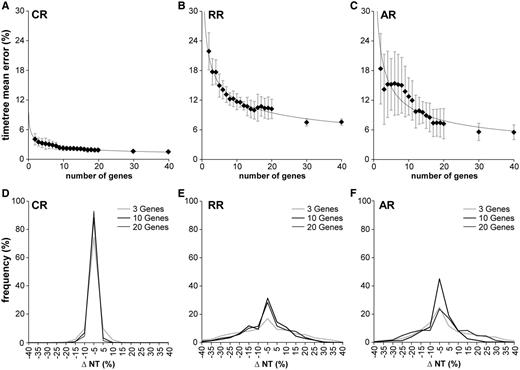
Error of divergence time estimates with increasing number of genes. Error (ΔNT) is measured as 100 × (H_EST − H_TRUE)/H_TRUE, where H_TRUE and H_EST are the true and estimated node heights (divergence times), respectively. (A–C) The mean estimation error for the entire tree by number of genes used for the different rate variation models. Error bars correspond to the standard deviation estimated from five replicates, each from a different sample of genes and rate assignments. In the CR case, only two genes are needed to achieve an average error of less than 5%. We used two additional, variable-rate models for sequence generation, RR and AR. In both of these cases, over 40 genes are needed to achieve a maximum average error of less than 5%, but only around 15 to bring error below 10%. (D–F) Distributions of the signed percentage divergence time estimation error of nodes for 1-, 3-, 10-, and 20-gene alignments. When more genes are used, the variance decreases, but a strong central tendency persists. In the CR and RR cases, there is little difference to be seen in the distributions between the 10- and 20-gene cases.

Open in new tabDownload slide

We then evaluated the error of time estimates under the other two rate models. Although AR and RR showed trends similar to CR, the average estimation errors for the AR and RR data sets were considerably greater (fig. 2A–C). The maximum error was over three times as large compared with the CR case and the slope was shallower. The presence of rate variation among lineages had a dramatic effect on the number of genes needed for more accurate time estimates, as AR and RR rate variation models did not achieve an overall average error rate of 5% even with 40 genes. It is important to note that the number of genes needed for reliable time estimates will vary from study to study. Although we have mentioned the average numbers of genes needed to achieve specified levels of accuracy, and used a large and realistic phylogenetic tree and genes with empirical evolutionary parameters, other particular data sets will have unique features and the same numbers may not apply. In such cases, though, the RelTime method is efficient enough to allow a succession of test runs with increasing numbers of genes to be done until time estimates are observed to stabilize.

In addition to the average overall error in the timetree, we also examined the distribution of errors observed for individual nodes for varying numbers of genes (fig. 2D–F). In CR simulations, we found that a large majority of nodes were timed with less than 5% error when three or more genes are used, none having more than 20% error. Therefore, a greater number of genes appear to be not required. In the variable-rate cases, however, there was still a strong central tendency, but the error distribution had more spread (up to a 40% error rate for a few nodes in the three-gene case). So, clearly a larger number of genes is necessary to obtain reliable estimates.

To explore the effect of missing data on divergence time estimation, we deleted a specified fraction of sequences randomly selected from each gene in the alignment. The percentage of sequences deleted is referred to as the sparseness in the data set, and its complement as the coverage in the data set. Figure 3A–C shows the effect of 20% and 60% sparseness on the mean error for data sets containing 2–40 genes. The effect of 20% sparseness on the average error was almost negligible, which is consistent with results from previous studies where the deletion of 25% of the data introduced, on average, less than 3% additional error (Douzery et al. 2004), see also Wiens and Morrill (2011), Wiens et al. (2012), and Roure et al. (2013). However, 60% sparseness had a considerable impact on the total error, which was substantially greater along the length of the curve and dropped near to the level of the 20% missing case only after 40 genes were used. In each case, the estimation error increased steadily with missing data for the given number of genes in CR, AR, and RR.

Fig. 3.

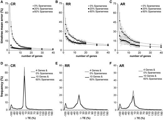
Effect of data sparseness on error. TE refers to time elapsed on a branch. (A–C) For each rate variation model and three different sparseness levels, the decline in error as more genes are added. In the CR case, there is virtually no difference between full data and 20% sparseness. 60% sparseness has considerably more error for fewer than ten genes, but as the number of genes increases, the error also converges to the full data levels. The RR situation is very similar but with error generally elevated over the CR case. AR shows a somewhat more pronounced difference between the full data and the 60% sparseness cases. (D–F) In these panels, we show the distributions of time estimate errors not for nodes, but for branches, in two cases, four genes with full data, and ten genes with 60% sparseness. In each case, there is the same number of sequences and taxa. We see that the distributions are virtually identical within each rate class, except for the left tail (−100% error case). These are cases in which the estimated branch lengths are zero. These are branches associated with nodes with zero data coverage (no genes with species in common to both child clades of the node). Such nodes have a substantial effect on mean error, but they can be easily detected a priori.

Open in new tabDownload slide

We also examined whether the properties of time estimation for empirical data are similar to that observed for simulated data by using a mammalian data set consisting of amino acid sequences from 162 taxa and 21 proteins (Meredith et al. 2011). In the original data set, sequences were available from each gene for each species (0% missing genes). In this case, we compared the estimates obtained using all the data with estimates using incomplete data (60% sparseness). Consistent with the computer simulated data, the results obtained with this sparse data were remarkably similar to those obtained using all available data (fig. 4A).

Fig. 4.

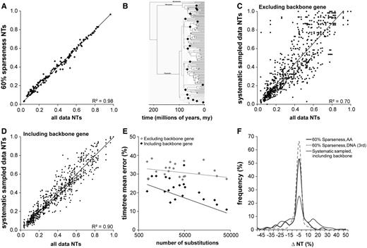
Results for amino acid divergence-time analyses of the 21-locus empirical data set of Meredith et al. (2011; see Materials and Methods for details). NT refers to relative time estimates of node divergence times. (A) Time estimate scatter diagram for analysis using the full set of 21 genes with 60% sparseness. In this case, because true divergence times are unknown, truth is taken to be the full-coverage case with all data. The R² coefficient of determination is 0.98. (B) Depiction of the mammalian clades used for the systematic sampling. Nineteen of the clades are marked by black diamonds, and the 20th is taken to be all of the remaining taxa. Each gene contains sequences for exactly two orders, assigned so that for each gene g₀, there exists exactly one gene g₁ and another gene g₂ such that g₀ shares exactly one clade with g₁ and the other clade with g₂. In this case, there is strictly limited species overlap among genes. We then added one “backbone” gene with a sequence for each taxon. The phylogenetic tree in the figure is based on the one that appears in Meredith et al. (2011). (C) Time estimate scatter diagram for analysis under the systematic sampling method described in the text, but without inclusion of the universal “backbone” gene. Again, truth is taken to be the full-coverage case with all data. (D) Time estimate scatter diagram for analysis under the systematic sampling method described in the text but in this case with the universal backbone gene. Resultant sparseness (percentage gaps in the data matrix) is approximately 90%. As before, truth is taken to be the full-coverage case with all data. We see that the R² coefficient (0.9) is much higher than in the case without backbone (0.7). (E) Effect of evolutionary rate of backbone gene on mean divergence time estimation error. Our mammalian data set contained 21 genes, each of which was used in turn as a backbone gene (black markers in the graph). The x axis represents the total number of substitutions observed for that gene and the y axis represents the total error of the resulting time tree. Gray markers represent 20-gene data sets without the backbone gene for each case (x value). Regression lines are fit to both sets of results and have R² values of 0.1 and 0.4 for the no-backbone and backbone case, respectively. We see that the use of the backbone gene is effective in reducing error and that faster-evolving backbone genes tend to be more effective than slowly evolving ones. (F) Distribution of signed error in the 60% sparse case when compared with the systematically sampled case with backbone. As we might expect from the fact that the systematic case is effectively 90% sparse, we see more spread to higher error in that case.

Open in new tabDownload slide

For the mammalian data, we also performed a more systematic form of sampling, because data availability for genes is sometimes highly variable among clades. In this case, we retained one randomly selected “backbone” gene with sequences for all species but sampled sequences from the remaining gene in such a way that no pair of genes had more than one mammalian order in common (see Materials and Methods for more detail). The resulting data set had approximately 90% sparseness, and multiple such data sets were generated. For this extreme case of missing data for 20 mammalian genes combined with one backbone gene, the time estimates showed a linear relationship with the times obtained from the fully sampled data set (fig. 4D). The overall accuracy with backbone was much better than the case where no backbone was used (fig. 4C). In the latter case, the error was 33% rather than 16%, and the correlation coefficient between the fully sampled and the systematically sampled data was reduced significantly (R² change from 0.98 to 0.70). Overall, the inclusion of a backbone gene along with many genes with systematic low coverage among clades produces results that appear to be quite similar to the case where genes are missing randomly among species (fig. 4F). Therefore, the average error in time estimation across the tree decreases substantially by adding a backbone (fully sampled) gene in the analysis of the sparse mammal data set. We found the decrease in error to be a function of the amount of information (substitutions) added by the backbone gene (fig. 4E), which is reasonable because slowly evolving, short genes will add less additional information when compared with faster evolving, long genes in the mammalian data set analyzed. The figure shows no significant relationship among the 21 replicates without backbone (gray markers), but when backbones are added, the error declines substantially, with the greatest reduction for the fastest evolving backbones.

Discussion

Using simulated sequence data based on realistic gene parameters and phylogenetic trees, we have found that the average divergence time estimation error declines with the number of genes used, as expected. We have also demonstrated that moderate amounts of missing data have a negligible effect on the accuracy of time estimates and that even data sets with a majority of genes missing for each species can yield good time estimates. We also found that the majority of error in data matrices with a high proportion of missing sequences is primarily due to a much higher error in estimating the time elapsed on some branches, many of which fall on the left tail of the histograms in the sparse case (ten genes with 60% sparseness) when compared with the full-coverage case of four genes with 0% sparseness (fig. 3D–F).

We explored the characteristics of the sparse data for nodes flanking these branches and found that these grossly underestimated branches were connected with clades for which the node data coverage was zero, that is, there were no genes for which sequences were available from at least one species from both of the child clades of the node (fig. 5). In these cases, no sequence data exist to estimate the length of such branches and the estimate of time elapsed on the associated branch became zero, resulting in a 100% underestimate (node with 0 in fig. 5). We refer to these nodes as having zero data coverage and the large error in their estimation contributes the great majority of the total error in the sparse data sets. We confirmed this trend in another way. Our simulation analysis of ten genes with 60% sparseness yields time estimates for nodes with varying levels of data coverage (0–10 genes). The error in the resulting estimates can be compared directly with time estimates for the respective nodes obtained using results from simulated data sets of one to ten genes with no missing data (0% sparseness). The amount of error normalized by the true divergence time in these two scenarios was very similar (fig. 6B–D), which means that the primary difference in accuracy between extremely sparse and complete data sets is caused by nodes with no (or very little) data coverage. These zero data coverage nodes tend to be at relatively shallow positions in the tree because of small clade sizes (fig. 6A) but some exist deeper in the tree because some deep nodes have one descendant with very few species. Fortunately, we can identify zero and low data coverage nodes based only on the sequence data and the tree topology by scanning the input sequence alignments. We recommend that the divergence times for such problematic nodes be presented as ranges of times from ancestral and descendant nodes with high data coverage. (Of course, the best solution is to reduce the sparseness of the data matrix.)

Fig. 5.

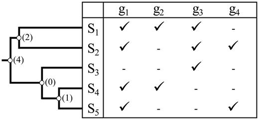
Node data coverage. The data coverage for any node in the phylogenetic tree is the number of genes that directly contribute to the time estimation for that node. A gene is considered to contribute to time estimation for a given node if it has sequences from at least one species pair, one each from the two immediate descendant clades. The figure shows a tree and corresponding data matrix, with genes g₁ to g₄ and species S₁ to S₅. Not all genes are available for each species. Available sequences are designated by check marks and missing ones are indicated by dashes in the matrix. Numbers in parentheses next to each node of the tree give the data coverage for that node. We may expect the time estimate for the node with zero data coverage to be very poor, since there is no sequence data to estimate the relevant branch length needed to estimate the divergence time. The best we can say is that it diverged at some time before either of its child nodes but after its parent node.

Open in new tabDownload slide

Fig. 6.

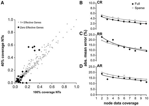
(A) A comparison of estimated divergence times based on ten genes and 60% sparseness is shown (RR rate model, other rate models give similar results). Nodes with zero data coverage are shown in black and have branch length time estimates of zero. These nodes are mostly shallow and have only a few species with data below them. (B–D) Relation between mean absolute value node time error and node data coverage for sparse (ten genes, 60% sparseness) and full coverage (zero sparseness, number of genes = node data coverage) in the CR, RR, and AR cases. The x axis is the node support and the y axis is the mean absolute value error for nodes with that amount of support. We see that, controlling for individual node support, there is very little, if any, difference in error between nodes in a sparse-coverage data set and in the full-coverage context.

Open in new tabDownload slide

It is not surprising that simply deleting data from the matrix increases the mean error. A more interesting comparison is made when two data sets have the same number of sequences but are allocated differently in the data matrix. For example, a ten-gene data set at 60% sparseness has as many gene sequences as a four-gene data set with no missing data (0% sparseness). The former incurs error rates of 7.5%, 19.0%, and 20.5% for CR, RR, and AR, respectively, whereas the latter has somewhat lower error rates of 3.5%, 17.7%, and 15.2%. So, there was some, but relatively little, added penalty for sparseness per se. We dissected these differences further by examining the distribution of the errors in the estimate of time elapsed on individual branches in the phylogenetic tree (fig. 3D–F). Interestingly, the error histograms were nearly identical within each rate model, except that there was a dramatic increase in the number of nodes with a 100% underestimate of time. On the other hand, we did not find any consistent trends of error differences between young versus old nodes and nodes with different number of species in the clade. For example, in an analysis averaging six simulated timetrees (CR, AR, and RR, full and sparse), and excluding nodes with zero data coverage, young (<40 Ma) two-species nodes show an error rate of 16%, which is similar to that of old (>190 Ma) two-species nodes (14%). Species-rich nodes (ten taxa) showed similar error rates to species-poor nodes (two taxa) (16% and 15%).

Although we have primarily discussed the influence of zero data coverage on the accuracy of divergence time estimation, we would expect our observations to apply to phylogenetic tree reconstruction when using sparse data as well. Nodes with zero data coverage will effectively lead to the zero-length branch problem in the “realized” trees, where the true phylogenetic partitions induced by such zero-length branches (not related to data sparseness) contributed extensively to the overall error, see Kumar (1996) and Kumar and Gadagkar (2000). However, to our knowledge, our way of dissecting the relationship of node-specific data coverage in sparse data sets and the accuracy of topological inference has not been presented in recent reports on the impact of missing data on the topological accuracy. Therefore, we are currently conducting computer simulations to investigate this phenomenon for inferring phylogenetic trees as well.

In conclusion, we have found that phylogenetic trees with several hundred taxa can be analyzed using RelTime to infer accurate estimates of many species-pair divergence times, even when individual species lack sequences for most genes in the matrix. When there are many missing sequences, it is necessary to avoid estimating times for nodes with no data coverage whatsoever, although times for other nodes may be estimated with varying degrees of accuracy depending on the number of genes contributing to the time estimate of each node. As expected, nodes with the highest data coverage give the most accurate estimates. We also found that when genes tend to be clade specific, it is advantageous to have at least one “backbone” gene with sequences for as many taxa as possible. Although many of these conclusions, such as the ones involving data coverage, seem method independent and so to apply to other approaches, for example, to BEAST (Drummond and Rambaut 2007), we were unable to test this directly due to the high-computational demands of some of these programs. It is best, therefore, to be cautious and only apply detailed results to the RelTime (Tamura et al. 2012) method studied here. Also, the impact of the use of an oversimplified (or incorrect) model of substitution, errors in the tree topology, or the reliability of fossil calibrations will likely have a substantial impact on the accuracy of times estimates. Therefore, we have begun a full-scale assessment of the degree of error introduced by such factors to better understand the quantitative impact of various realities of practical data analysis. However, we expect the observations made here about the effect of missing data and the node data coverage on time estimation to be qualitatively applicable in general.

Materials and Methods

Computer Simulation

We conducted computer simulations to generate nucleotide sequence alignments from a 446-taxon tree, which was derived from the bony-vertebrate clade in the Timetree of Life from which all polytomies were pruned (fig. 1A) (Tamura et al. 2012). Figure 1 legend contains a descriptive summary of characteristics of the data. The distribution of node divergence times is shown in figure 1B (Tamura et al. 2012). Gene lengths (fig. 1C) and other evolutionary parameters were drawn from empirically derived data on the number of sites (range 445–4,439 sites), nominal per-gene evolutionary rates (range 1.35–2.60 substitutions/site per billion years), GC content (range 39–82%), and the transition/transversion ratio (range 1.9–6.01) (Rosenberg and Kumar 2003). Independent sets of sequence simulations, with five replicates each, were performed using CR, AR, and RRs among lineages following the procedures in Tamura et al. (2012). In brief, the actual number of substitutions on a branch in the model tree was determined according to a Poisson process with the mean equal to the expected number of substitutions (determined by average rate and sequence length) in the CR case. In the AR scenario, evolutionary rates among lineages were autocorrelated following Thorne and Kishino (2002) using autocorrelation parameter ν = 1 (Kishino et al. 2001). The RR case was simulated with the branch-specific evolutionary rate drawn from a uniform distribution over the open interval 0−2r, where r is the original nominal rate for the entire gene. No within-sequence insertions or deletions were performed. We used SeqGen (Rambaut and Grassly 1997) under the Hasegawa–Kishino–Yano (HKY) model (Hasegawa et al. 1985) to generate the simulated sequences. Rate variation was accomplished by using a special-purpose program to modify branch lengths in the manner described above in the trees given to SeqGen for simulation. For multigene analyses, gene alignments were generated separately and concatenated to form supergenes. When sparse matrices were needed, the required number of individual sequences was selected at random and corresponding sites were replaced by missing data characters in the supergenes. Figure 1D shows the resulting distributions of per-branch rates, where the nominal rate for each gene is normalized to 1.0, so that the values on the x axis are rate (speed-up or slow-down) factors. On the same graph, the distribution for the CR case would be a single spike at 1.0. The distributions show how the factors vary over many branches in many trees but do not show how the branch lengths are autocorrelated in the AR case.

Molecular Dating Analyses

In all analyses of the simulated data sets, we used the correct general model (HKY with five gamma rate-variation categories among sites) of nucleotide substitution and the correct phylogeny. Time estimates were performed using the RelTime feature of MEGA 6.0 with maximum-likelihood branch length estimation and the “use all sites” data option (Tamura et al. 2013). RelTime is already known to perform well, does not require knowledge of the distribution of the lineage rate variation a priori, and does not require calibration times or their associated distributions to obtain relative time estimates of internal tree nodes, although these relative times can be converted to actual times if one or more calibration points (from fossil data or from other sources) are provided (Tamura et al. 2012, 2013). This means that RelTime produces relative times of divergences for all nodes in the given phylogenetic tree, which can be directly compared with the true relative times that come from the model tree used to simulate the sequences. All comparisons of estimated and true times involved relative (not absolute) values. Node heights were normalized by dividing by the sum of all node heights in the tree. We calculated the percent error (ΔE) between the normalized true node height (T) and the normalized estimated height (E) as ΔE = 100 × (E–T)/T. All runs were done on an Intel Xeon 2.4 GHz processor under Windows Server 2012. RelTime run times for the 446-taxon analyses ranged from 3 processor-minutes for single-gene analyses to 22 processor-hours for the longest concatenations (60 kb). Runtimes were approximately linear on the number of genes.

Mammalian Data

We also examined whether the properties of time estimation for simulated data are similar to that observed for empirical data by using a mammalian data set consisting of amino acid sequences from 162 taxa and 21 proteins (Meredith et al. 2011). With this data set, we performed two kinds of sequence sampling. In the first, we simply deleted at random, as before, a specified proportion of sequences in the data matrix, replacing those by sequences of indel characters in the final supergenes given to RelTime. Second, we performed a more systematic form of sampling in which we retained, for each replicate, one randomly selected “backbone” gene with sequences for all species, but sampled sequences from the remaining genes in a clade-specific way. This was meant to reflect the situation where scientists have one or a few widely sequenced genes with full-species coverage and then some more clade-specific genes. We implemented this by partitioning the set of species in the mammalian data set into 20 disjoint subsets, roughly corresponding to mammalian orders (fig. 4B). Then, we selected a gene at random to serve as “backbone” and randomly assigned clades to each of the 20 remaining genes in such a way that 1) each nonbackbone gene was associated with exactly two clades, 2) each clade was associated with exactly two nonbackbone genes, and 3) each nonbackbone gene shared exactly one clade with one other nonbackbone gene and no clades with any of the other nonbackbone genes. The complete sequence data from the remaining gene was then added to the alignment. The resulting data sets had approximately 90% sparseness.

Acknowledgments

This work was supported by the National Institutes of Health (NIH) HG002096-12 to S.K. and HG006039-02 to A.F., National Science Foundation DBI-0850013 to S.K. O.M. was supported by a training program (NIH R25 GM099650).

References

Author notes