MISFITS: Evaluating the Goodness of Fit between a Phylogenetic Model and an Alignment Free

Abstract

Introduction

In recent years, the complexity of models of sequence evolution steadily increased (cf. M Swofford et al. 1996, Felsenstein 2004). The general time reversible model (GTR) allows for the estimation of nucleotide-specific substitution rates (e.g., Yang 1994), the assumption of different rates across sites is included (e.g., Yang 1993, Gu et al. 1995) and even heterogeneity and change in evolutionary substitution models along a tree can be modeled (e.g., Tuffley and Steel 1998, Foster 2004). Moreover, we are able to compute the likelihood of a tree by using rapid maximum likelihood (ML) tree reconstruction methods (Huelsenbeck and Ronquist 2001, Guindon and Gascuel 2003, Jobb et al. 2004, Minh et al. 2005, Stamatakis et al. 2008). Tools are also available to select the best model from a collection of available models (Posada 2008). Recent surveys (Sullivan and Joyce 2005, Ripplinger and Sullivan 2008) indicate that the most complex model is typically selected. The selected model leads to a tree that has a significantly higher likelihood than trees based on the other models.

The next step in a regular phylogeny analysis would be to test how well the selected model fits the alignment. The easiest such approach is a parametric form of the classical likelihood ratio statistics, where the likelihood of the tree is compared with the unconstrained likelihood (Navidi et al. 1991, Goldman 1993a, 1993b). Due to its computational costs and possibly also due to the unpleasant outcome that the tree does not explain the alignment very well, the test is typically not applied. However, it has been shown that a careful combination of such tests and then subsequently going back to the alignment can help to improve the phylogenetic analysis (Schöniger and von Haeseler 1999). Nevertheless, this analysis was instance based and it is not possible to apply it routinely to alignments.

Thus, there is a need to suggest an applicable method that tests whether the alignment is explained adequately by the model and the inferred tree. The method should simultaneously suggest alignment positions that may not fit to the model and the tree. We present such a method, the so-called MISFITS, in this paper.

In a nutshell, MISFITS does the following: Based on the alignment, the substitution model, and the inferred ML tree, we compute the likelihood of the site patterns in the alignment and the corresponding unconstrained likelihood (Navidi et al. 1991, Goldman 1993a,1993b). A confidence region is then computed to determine a set of overrepresented patterns and a set of underrepresented patterns with respect to the expected number of occurrence. We then apply a maximum parsimony approach to determine the minimal number of extra substitutions on the ML tree necessary to convert an alignment column that belongs to an overrepresented pattern into a pattern that is underrepresented in the alignment. The theoretical basis to compute the minimal number of substitutions utilizes the concept of one-step mutation (OSM) matrices (Klaere et al. 2008). Subsequently, a parametric bootstrap analysis is performed to determine whether the number of extra substitutions is significantly elevated. Moreover, the overrepresented patterns are mapped back to the alignment to pinpoint to potentially problematic regions in the alignment and to enable a more thorough analysis.

We give a series of illustrative examples and a survey about the goodness of fit of the selected models to the alignments as provided by the PANDIT database (Whelan et al. 2006).

Methods

Table 1 presents a schematic workflow of MISFITS. We will now describe the steps in more detail.

Steps 1 and 2: Consider a gap free, multiple nucleic acid alignment of n sequences with length ℓ, a nucleotide substitution model, and the inferred ML tree. For n taxa, a total of 4ⁿ site patterns are possible. The sites of the alignment constitute a subset of these patterns. Given the ML tree and the substitution model (thereafter jointly referred to as tree model), we compute the expected pattern likelihood vector (p^tree) for the patterns in the alignment using, for example, IQPNNI (Minh et al. 2005), Tree-Puzzle (Schmidt et al. 2002), and PHYML (Guindon and Gascuel 2003). The unconstrained likelihood vector (p^unc) of the patterns is simply the number of alignment sites showing the pattern divided by the length of the alignment (Navidi et al. 1991, Goldman 1993a, 1993b). p^unc is actually the observed frequency of the patterns in the alignment. Thus, it will be called observed pattern frequency vector.

Step 3: If the ML tree is an adequate description of the data, the difference between the two vectors p^tree and p^unc should be small. In fact, they are the basis for the Cox test suggested by Goldman (1993b). Instead of looking at the overall fit, we compare the two vectors position wise. Figure 1 displays a parametric plot of the logarithms of the two likelihood vectors computed on a primate complete mitochondrial genome data set under the GTR model. The x axis displays the logarithm of the entries in p^tree and the y axis the logarithm of the unconstrained likelihood p^unc. If the tree model describes the data adequately, all points will approximately lie on the identity line. However, residuals (deviation from the identity line) are often observed. To account for variability in the data, we compute a simultaneous α = 95% Gold confidence region for multivariate proportions (Gold 1963) for the entries in p^tree:

is the confidence interval for the likelihood of pattern i (p_i^tree) under the tree model, where κ² = χ_k²(α/(2ℓ)) is the 1 − α/(2ℓ)-quantile of the χ² distribution with k degrees of freedom. The degrees of freedom in this case are the total number of estimated variables, that is, the sum of the number of parameters of the substitution model and the number of branches on the ML tree. The dashed lines in figure 1 show the logarithms of the upper bound and the lower bound of the confidence region.

FIG. 1.

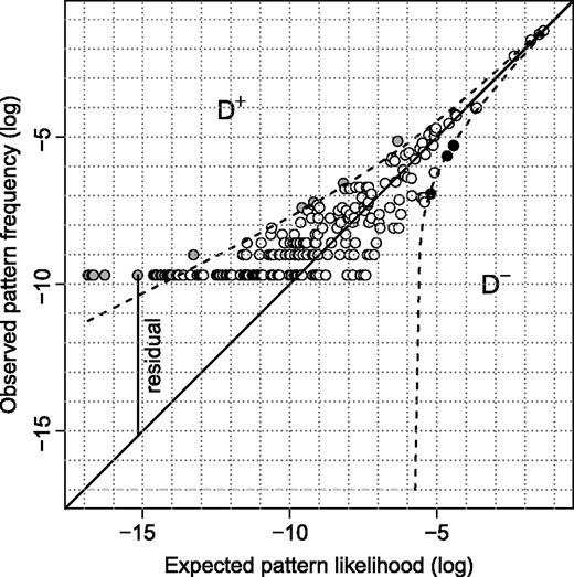
Observed pattern frequencies and expected pattern likelihood under the tree model. Each circle represents a pattern in the alignment by its expected log likelihood under the tree model (x axis) and the logarithm of its frequency or unconstrained likelihood (y axis). The dashed lines indicate the 95% Gold confidence region. The open circles represent patterns within the confidence region; the black-filled circles are underrepresented patterns, whereas the gray-filled circles are overrepresented patterns.

Open in new tabDownload slide

FIG. 2.

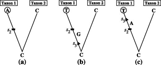
Placing an extra substitution on a branch. Figure (a) shows a rooted two taxon tree, where the mutation history of the nucleotide position is known: A substitution s₂ occurred on the branch leading to taxon 1. An extramutation s₃ was introduced (b) before and (c) after the substitution s₂ occurred. Wherever the extra substitution s₃ was placed, the nucleotide observed in taxon 1 is the same.

Open in new tabDownload slide

We call pattern i overrepresented if p_i^unc is greater than the upper bound of CI(p_i^tree). If p_i^unc is smaller than the lower bound of CI(p_i^tree), then pattern i is underrepresented in the alignment. We denote the set containing the overrepresented patterns 𝒟⁺ and the set of the underrepresented patterns 𝒟⁻. 𝒟⁻ also contains patterns not observed in the alignment, where the pattern likelihood under the tree model is larger than 1/ℓ. Thus, we would expect to find them at least once in an alignment of length ℓ. These patterns can be easily constructed using the OSM matrix (Klaere et al. 2008).

The overrepresented site patterns indicate alignment sites that occur more often than expected under the tree model. This means that the tree model does not capture these alignment sites adequately. On the other hand, the underrepresented patterns are expected to occur more often in the alignment than they actually do. Thus, it appears plausible to compute the minimal number of substitutions that are required to change the overrepresented sites in the alignment (site patterns in 𝒟⁺) into patterns that are more likely to occur given the ML tree (patterns in 𝒟⁻). The number of extra substitutions can then be used as a measure to evaluate the goodness of fit of a model to the data: the less the number, the better the fit.

Step 4: We now describe how to compute the extra substitutions to convert a pattern into another pattern. The mathematical intricacies will be described elsewhere (Klaere S, Nguyen MAT, and von Haesler A, in preparation). For this work, it suffices to recapitulate the Kimura three-parameter model (Kimura 1981). It distinguishes three types of substitutions as summarized in the following permutation matrices:

where s₁ describes the transitions within purines and pyrimidines, respectively, s₂ represents the transversions within the nucleotide pairs (A,C) and (G,T), and s₃ the remaining transversions within the nucleotide pairs (A,T) and (C,G). Using this model, we now study the effect of an extra substitution on a certain branch of the tree. Consider the rooted two taxon tree in figure 2. The mutation history of the nucleotide on this tree is known: The root state is C and a substitution s₂ occurs on the branch leading to taxon 1. Therefore, we observe the nucleotide A in taxon 1. How will the observed nucleotide change if we introduce an extra substitution, for example, an s₃ substitution, on the branch leading to taxon 1? We can introduce s₃ either “before” or “after” s₂ occurs. If the extra substitution s₃ occurs before s₂, it changes the root nucleotide C into G. Then, G is changed into T by s₂; hence, T would be observed in taxon 1 instead of A (see fig. 2b). If the extra substitution occurs after s₂, it changes the observed nucleotide A also into T (fig. 2c). Thus, independent of the order of substitutions, the outcome is always a T at taxon 1. Hence, placing an extra substitution on an edge of the tree results in a unique outcome independent of the unknown substitution history of the observed nucleotide. This is essentially due to the fact that the substitution matrices s₁,s₂,s₃, and the identity matrix s₀ form a commutative group (Klein four group) with respect to matrix multiplication. We also note that the Kimura three-parameter model is the most general model for nucleotide substitution that can be used in our approach.

The algebraic structure of the Kimura model also allows for an efficient way to convert an alignment pattern p into another pattern p^′ by putting a minimal number of extra substitutions on the tree. In a straightforward approach, one could simply generate all possible patterns from p by putting a number of extra substitutions on branches of the tree until p^′ is produced. However, this approach is computationally infeasible. Klaere S, Nguyen MAT, and von Haesler A (in preparation) show that a parsimony algorithm produces the required number of extra substitutions. Here, we discuss an example. Consider the rooted four taxon tree in figure 3a and the pattern GTAA at the leaves. Assume that the pattern GTAA is to be converted into ACAA. By comparing patterns position wise, we need a substitution s₁ on the branch leading to taxon 1 to convert G into A at the first position (the first taxon). Similarly, we need a substitution s₁ on the branch leading to taxon 2; no changes are needed for taxa 3 and 4. Thus, a series of substitutions (s₁,s₁,s₀,s₀) on the four external branches of the tree transfers the pattern GTAA into the pattern ACAA. Because taxa 1 and 2 form a cluster on the tree and the two substitutions are from the same matrix s₁, they are equivalent to a substitution s₁ on the corresponding internal branch. As shown before, the outcome is independent of the order of the extra substitutions to the unknown substitutions; therefore, the extra substitution s₁ on the internal branch is enough to switch the pattern GTAA into the pattern ACAA.

FIG. 3.

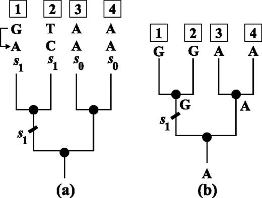
Exchanging two patterns on the tree. Figure (a) displays a rooted four taxon tree with a pattern GTAA observed at the leaves. If we want to convert the pattern GTAA into ACAA, we may introduce a series of substitutions (s₁,s₁,s₀,s₀) to the four external branches. Under the Kimura three-parameter model and the OSM setting (Klaere et al. 2008), this series is equivalent to an “extra substitution” s₁ on the internal branch leading to taxa 1 and 2 as the two taxa form a cluster on the tree. Therefore, the one extra substitution is enough to switch the observed pattern GTAA into ACAA regardless of the evolutionary process the pattern GTAA has undergone. On the other hand, the above substitution series converts a constant pattern AAAA into a unique pattern GGAA. Hence, converting the pattern GTAA into ACAA is equivalent to evolving the ancestral character A along the tree such that pattern GGAA is obtained at the leaves. Applying the Fitch algorithm (Fitch 1971) to the latter results in a unique assignment in (b): An s₁ substitution, which changes A into G, occurs on the internal branch leading to taxa 1 and 2. This assignment is identical to the assignment in (a).

Open in new tabDownload slide

FIG. 4.

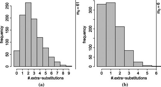
Primate complete mitochondrial genome. Histogram of the number of extra substitutions computed on 1,000 generated alignments under (a) GTR and (b) GTR + I + Γ models. The attained value (m₀) was significantly high under both models.

Open in new tabDownload slide

On the other hand, Klaere et al. (2008) showed that the series of substitutions (s₁,s₁,s₀,s₀) can also act on any other pattern and produces another unique pattern. Applying this series of substitutions on a constant pattern, AAAA, leads to the pattern GGAA. Therefore, converting the pattern GTAA into the pattern ACAA is equivalent to converting the constant pattern AAAA into the pattern GGAA. Hence, computing the minimal number of substitutions to change the pattern GTAA into the pattern ACAA is equivalent to computing the minimal number of character changes required along the tree to explain the pattern GGAA observed at the leaves given that the root state is A. The latter can be efficiently computed using the Fitch algorithm (Fitch 1971) with the extension that if the root character set does not contain A, we increase the number of character changes by 1. The Fitch algorithm also assigns the substitutions on the branches of the tree. In our example, this results in an unique assignment in figure 3b, which agrees to the assignment in figure 3a.

Step 5: After computing the number of substitutions to convert each pattern in 𝒟⁺ into every pattern in 𝒟⁻, we determine a matching which pairs every pattern in 𝒟⁺ with patterns in 𝒟⁻ such that the total number of substitutions is minimal. This is done by applying the Munkres algorithm for the assignment and transportation problems (Munkres 1957). The minimal number of substitutions, thereafter referred to as the number of extra substitutions and denoted as m, is then considered as the minimal “cost” to fit the tree model to the observed data.

Step 6: Subsequently, we apply the second part of the Fitch algorithm to assign extra substitutions to the branches of the tree to exchange the paired patterns between 𝒟⁺ and 𝒟⁻.

Step 7: Finally, we assess the significance of the number of extra substitutions using parametric bootstrap. We generate a number of alignments (e.g., 1,000 alignments) on the tree under the substitution model with the respective parameter values using a sequence generator program such as Seq-Gen (Rambaut and Grassly 1997). We then re-estimate the tree and compute the number of extra substitutions for each simulated alignment. Subsequently, we determine whether the number of extra substitutions computed on the original alignment (m₀) is significantly high according to a given significance level (5%). It should be noted that if m₀ is close the critical value (5% point), one may increase the number of simulated alignments for a more accurate estimation of the P value.

Results

Primate Mitochondrion, Complete Genome

The data set under consideration contains the complete mitochondrial DNA from five primates: chimpanzee, bonobo, human, gorilla, and orangutan (Horai et al. 1995). The alignment, after removing sites containing gaps, is 16,271 bp long and is composed of 241 distinct patterns. As discussed earlier, figure 1 shows the logarithm of the observed pattern frequencies and the expected pattern likelihood under the GTR model. We counted 207 patterns within the confidence region (open circles), 30 overrepresented patterns (gray-filled circles), and 4 underrepresented ones (black-filled circles). Using the OSM matrix (Klaere et al. 2008), we generated 94 patterns one substitution away from the constant patterns, 12 of which are not observed in the alignment but are all expected to occur at least once. The average likelihood of these 12 patterns is 1.09×10 ^{− 4}, whereas the average likelihood of the 25 overrepresented patterns, each occurring once in the alignment, is 5.28×10 ^{− 7}. Thus, the unobserved one substitution patterns are on average 207.5 times more likely to occur in the alignment. The inferred ML tree is rooted at the external branch leading to the orangutan and the resulting number of extra substitutions was 61. This was excessively high compared with the simulated null hypothesis distribution (fig. 4a).

We then included invariant sites (I) and Γrate heterogeneity into the GTR model and also examined a simpler model, JC69 + I + Γ. Under JC69 + I + Γ, the number of extra substitutions on the original alignment (m₀) was 2,168 and it was way out of the range of the simulated null hypothesis distribution (data not shown). Remarkably, m₀ estimated under GTR + I + Γ, though very low (m₀ = 6), was still significantly high (Pvalue = 0.002 based on 1,000 simulated alignments, fig. 4b). This demonstrates the power of our approach in terms of rejecting models that do not really fit the data.

This study involves a simple model, JC69 + I + Γ, and the more complex ones, GTR and GTR + I + Γ. Nevertheless, these models are rejected by the Cox test proposed by Goldman (1993b) (data not shown) as well as under our approach. Thus, there might be factors in the process of evolution that even the complicated model GTR + I + Γ was unable to cover. A closer look at the data revealed four overrepresented site patterns. Two of which are located at genes ND1 and ND5, both at the third codon position: position 747 in the human ND1 gene and position 981 in the human ND5 gene (positions 4,053 and 13,317, respectively, in the human mitochondrial genome). The other two are located at the D-loop at positions 151 and 16,293 in the human mitochondrial genome. Moreover, it should be noted that the test of homogeneity of the substitution process on a phylogeny advocated by Weiss and von Haeseler (2003) also rejected GTR and GTR + Γ on this data set. It implied that there may be heterogeneous substitution processes within the phylogeny describing the data.

Fungi, Metazoa CDC45-Like Region

This protein-coding DNA alignment (PF02724) was taken from the PANDIT database (Whelan et al. 2006). It encodes the CDC45-like protein. The sequences are homologs, as studied by Saha et al. (1998), from seven fungi, metazoa species: Ustilago maydis (Corn smut), Saccharomyces cerevisiae (Budding yeast), Schizosaccharomyces pombe (Fission yeast), Caenorhabditis elegans (C. elegans), Drosophila melanogaster (Fruit fly), Xenopus laevis (Xenopus), and Homo sapiens (Human). After removing sites containing gaps, 1,503 sites remain.

Model testing under Akaike information criterion suggested the GTR + I + Γ model. However, the inferred tree failed to recover the generally accepted taxonomic groupings (fig. 5a). The internal branch leading to one of the inappropriate groupings (Xenopus, C. elegans) is weakly supported by 31%. Remarkably, the tree inferred by a simpler model, JC69 + I + Γ, was congruent with the generally accepted phylogeny (fig. 5b). Moreover, this tree needs 15 extra substitutions less than the tree in fig. 5a. Figure 5a and b also display the assignment of the extra substitutions on the trees using accelerated transformation, ACCTRAN (Farris 1970, Swofford and Maddison 1987). The number above each branch shows the number of extra substitutions. Branch lengths are scaled according to the number of substitutions per site under the ML estimation. The root was placed on the branch separating the fungal species from the metazoa.

FIG. 5.

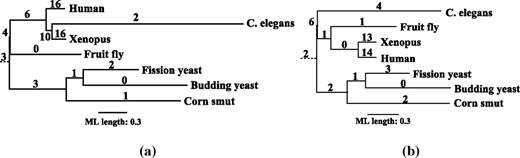
Fungi, metazoa CDC45-like region. Figures (a) and (b) present the ML trees reconstructed under GTR + I + Γ and JC69 + I + Γ, respectively. Branch lengths are scaled according to the ML estimation. The number above each branch is the number of extra substitutions assigned by MISFITS.

Open in new tabDownload slide

FIG. 6.

Fungi, metazoa CDC45-like region. Histogram of the number of extra substitutions computed on 1,000 generated alignments under (a) GTR + I + Γ, (b) JC69 + I + Γ, and (c) GTR models. The attained value (m₀) falls in the null hypothesis distribution (not significant) under GTR + I + Γ and JC69 + I + Γ. It is significantly high under GTR though (c).

Open in new tabDownload slide

Notably, we observed the tendency to place extra substitutions on short branches, for instance, on the two external branches leading to Human and Xenopus. A reason may be that substitutions on short branches are rarely captured by the ML model. They are then accounted for by our approach as extra substitutions. We therefore studied the significance of the number of extra substitutions assigned to the branches of the tree under JC69 + I + Γ. We generated 1,000 alignments, used them to re-estimate the branch lengths and then computed the number of extra substitutions on the branches of this tree. Table 2 displays the results. The number of assigned extra substitutions on all branches of the tree, including the two external branches leading to Human and Xenopus, are not significantly high (significance level α = 0.05).

Highlighting the overrepresented positions in the alignment, we observed most of them at the third codon position: 88.6% under GTR + I + Γ and 87.5% under JC69 + I + Γ. This is congruent with the fastest evolutionary rate of the nucleotides at the third codon position (M Swofford et al. 1996, Rodríguez-Trelles et al. 2006, bofkin2007).

Finally, we studied the significance of the number of extra substitutions on the trees under the above two models and GTR (1,000 alignments were generated for each model). Under JC69 + I + Γ and GTR + I + Γ, the number of extra substitutions (m₀ = 49 and 64, respectively) fell in the corresponding simulated null hypothesis distribution (no significance). However, m₀ = 196 under GTR was way too high (see fig. 6). It implies that models without rate heterogeneity across sites would be inadequate for this data set.

Most importantly, this alignment demonstrates a case in which a simpler model, JC69 + I + Γ, performed better than a more complex one, GTR + I + Γ, with regards to the inferred trees (cf. Sullivan and Swofford 2001) and to the number of extra substitutions. Thus, MISFITS is capable of indicating such a situation.

Study on a Large Range of Data

We applied MISFITS to study a wide range of multiple alignments of protein-coding DNA sequences from the PANDIT database, release 17 (Whelan et al. 2006). The PANDIT database contains 7,738 alignments in total. Alignments with less than four sequences (1,247 alignments) were discarded from our analysis as the tree space (only one shape) and the pattern space (not more than 64) are too small for a typical phylogeny analysis. Alignments with more than 100 sequences (320 alignments) were also discarded because the gapless alignment lengths are too short: The average of gapless alignment sites per taxon (alignment length divided by number of sequences) is 1.23. Alignments with short sequence length and large number of taxa may lead to a bias in phylogeny inference (Revell et al. 2005). Thus, the study involved 6,171 alignments containing from 4 to 100 sequences with gapless alignment length ranges from 15 to 6,288 bp. The discarded alignments are listed in supplementary table S1, Supplementary Material online.

First, we used jModelTest (Posada 2008) to select the best model for each alignment. Under the selected model, the ML tree and pattern likelihood were computed by using the PHYML package (Guindon and Gascuel 2003) and the PUZZLE program (Schmidt et al. 2002), respectively. We observed that the GTR models with and without rate heterogeneity across sites (GTR, GTR + I, GTR + Γ [four rate categories], GTR + I + Γ) were mostly selected (70.65%). Furthermore, models with one rate across sites were rarely selected (only 1.54%, see table 3).

Subsequently, we studied the goodness of fit of the selected models to the alignments. For 777 alignments (12.59%), the observed frequencies of all patterns are within the confidence region. The number of sequences in these alignments ranges between four and eight. Thus, for alignments with more than eight sequences, 𝒟⁺ or 𝒟⁻ are never empty. The number of extra substitutions needed for these 777 alignments is 0.

FIG. 7.

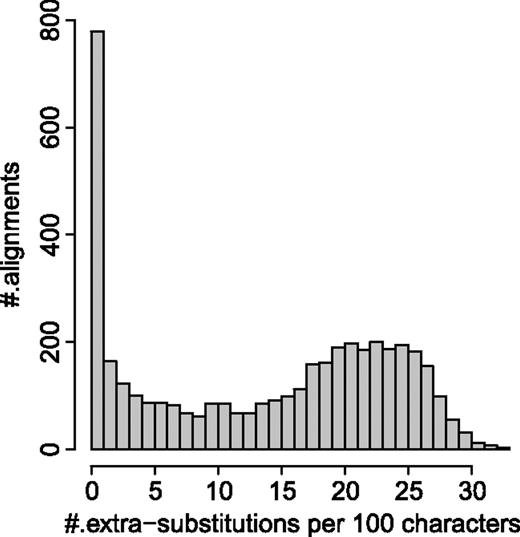
Results on PANDIT database under the selected models for the 4,268 alignments where overrepresented patterns were observed and there were enough underrepresented patterns to exchange with them. The histogram displays the number of alignments (the y axis) versus the number of extra substitutions per 100 characters (the x axis).

Open in new tabDownload slide

FIG. 8.

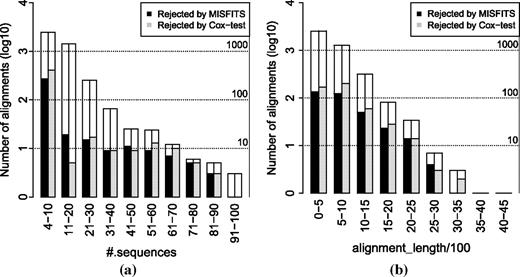
Results on PANDIT database under the selected models for the 4,268 alignments where overrepresented patterns were observed and there were enough underrepresented patterns to exchange with them. The height indicated by the nonfilled bars display the number of alignments in logarithm to base 10 (the corresponding decimal values are depicted by the dashed horizontal lines together with the numbers on the right). The filled bars show the number of alignments (models) being rejected by MISFITS (black bars) and by the Cox test proposed by Goldman (gray bars) with respect to the number of sequences in the alignment (a) and to the alignment length (b).

Open in new tabDownload slide

We observed overrepresented patterns in the remaining 5,394 alignments. There were 98 alignments in which all patterns are overrepresented. Thus, not a single pattern fell into the confidence region. This is attributed to the fact that they contain only singleton patterns (occurring only once in the alignment). Phylogeny based on such alignments with tremendously diverse patterns is probably arbitrary. Therefore, we discarded these alignments from the next steps.

The next step of MISFITS thus comprised 5,296 alignments. However, for 1,028 alignments (19.41%), there were not enough unobserved patterns having a likelihood greater than 1/ℓ, that is, not enough underrepresented patterns to exchange for all the overrepresented patterns. These alignments were also discarded. These alignments together with the above 777 and 98 alignments are listed in supplementary table S2, Supplementary Material online.

Thus, 4,268 alignments went into the final analysis. The percentages of the models being selected for these alignments were similar to those in table 3. Thus, the removal of the above alignments did not change the model selection substantially. On average, MISFITS introduced 13.73 extra substitutions per 100 characters (number of extra substitutions per site divided by the number of sequences in the alignment times 100). Figure 7 shows the histogram of the number of alignments against the number of extra substitutions per 100 characters.

Based on the parametric bootstrap analysis consisting of 100 simulations for each of the 4,268 alignments, MISFITS showed that the number of assigned extra substitutions was not significant for 3,918 alignments (91.80%) and significantly high for 350 alignments (8.20%). This means our approach would reject 350 models. The Cox test proposed by Goldman (1993b) rejected 478 models (11.20%), which is in the same order of magnitude (refer to supplementary tables S1 and Supplementary Data, Supplementary Material online for more details on these 3,918 and 350 alignments, respectively). Two-hundred and seventeen models were rejected by both approaches. Figure 8a and b display the number of alignments (the height indicated by the nonfilled bars) and the number of alignments (models) being rejected by MISFITS (black bars) and by the Cox test proposed by Goldman (gray bars) with respect to the number of sequences in the alignment (a) and to the alignment length (b). These figures (see also Supplementary figs. S3 and Supplementary Data, Supplementary Material online) show that the proportion of models being rejected by both methods tends to increase when the number of sequences grows as well as when the alignment length becomes longer. This implies that it becomes more and more difficult to have a single model that can adequately explain the data.

We learned from this survey that in a number of instances (8.20%), the selected models and the resulting trees do not really fit the data. Moreover, typically singleton patterns are overrepresented. One reason for this is the discrete nature of the patterns. Occasionally, some patterns have a very small likelihood to occur on the inferred tree. Therefore, it is more plausible to explain the occurrence of such a pattern by extrasubstitutions, which are not covered by the model but are more likely to happen on the tree.

Discussion

MISFITS provides a guided efficient way to pinpoint to site patterns in the alignment, which are not captured well by the substitution model and the inferred tree (refer to supplementary section 1, Supplementary Material online for further details). The differences (residuals) between their observed frequencies and the corresponding expectation manifest themselves in a clear deviation from the identity line (cf. fig. 1). We then introduced a computational feasible method which puts extra substitutions on the tree to reduce the residuals. The extra substitutions reduce overrepresented site patterns in the alignment and at the same time increase underrepresented patterns. This has the ultimate effect that these extra substitutions pull overrepresented patterns and simultaneously push underrepresented patterns into the confidence region.

A big advantage of the approach is the possibility to map the extra substitutions on the tree. Moreover, the extra substitutions required give a biological interpretation why the data may not be adequately described by the tree model. The reasons for significant deviations, however, may be different for every single instance. They depend on the selected sequences, the selected organisms, and the unknown evolutionary history of the sequences. This needs to be elucidated on a case-by-case basis. Nevertheless, our tool on the one hand may point to potential regions in the alignment that may deserve a closer analysis. On the other hand, the assignment of extra substitutions to branches of the tree provides additional information to the interpretation of the inferred phylogeny: where on the tree such extra substitutions would help to reduce the residuals.

The approach we suggest also sheds additional light on the goodness of fit in model testing approaches that are discussed, for example, by Goldman (1993b) and Posada (2008). It even may point to the risk of overfitting the data that may lead to biologically implausible results such as in the fungi, metazoa CDC45-like region example.

From the computational point of view, it is practical in terms of running time to apply MISFITS routinely to alignments. First, the computational complexity required to find the number of substitutions that change a pattern in 𝒟⁺ into a pattern in 𝒟⁻ is indeed the complexity of the preliminary phase in the Fitch algorithm, that is, O(n), where n is the number of sequences (Fitch 1971). Thus, computing the number of substitutions for every pair of patterns between 𝒟⁺ and 𝒟⁻ has complexity O(n·|𝒟⁺|·|𝒟⁻|), where |·| denotes the cardinality of a set. Second, finding an optimal matching between patterns in 𝒟⁺ and 𝒟⁻ such that the total number of extra substitutions is minimal according to the Munkres algorithm runs in the worst-case time O(V³), where V = max{|𝒟⁺|,|𝒟⁻|}. Moreover, the number of patterns in 𝒟⁺ is not larger than the number of distinct patterns observed in the alignment. The number of distinct patterns in the alignment cannot exceed both the alignment length and the total number of possible patterns (4ⁿ). Hence, |𝒟⁺| ≤ M = min{ℓ,4ⁿ}. The cardinality of 𝒟⁻ is in the same order of magnitude with the cardinality of 𝒟⁺, as 𝒟⁻ contains patterns whose likelihood under the tree model is larger than 1/ℓ. Therefore, in the worst case where all alignment sites are distinct and overrepresented, computing the number of substitutions for every pair of patterns and then finding the optimal matching between 𝒟⁺ and 𝒟⁻ requires O(nM²) and O(M³) complexity, respectively. Nevertheless, although studying alignments with a large number of sequences from the PANDIT database, we never observed 4ⁿ patterns in the alignment. On average the computation of m₀ for one of the 4,268 alignments going through all analysis steps took 8.4 s on a single core of a 3-year-old dual core AMD Opteron CPU 2220 SE. A more detailed depiction of the computing time with respect to sequence length and number of sequences is given in the Supplementary figure S5, Supplementary Material online.

We have discussed so far the biological implications and the computational complexity MISFITS may cause. It should be noted that there is also room for methodological extensions. For example, different locations of the root on the tree may result in different numbers of extra substitutions as there is a constraint about the character state at the root while employing the Fitch algorithm in our approach. It is feasible to implement an exhaustive or heuristic search for the location of the root which gives the minimal number of extra substitutions. However, it is more useful to provide a biologically meaningful rooting based on preliminary knowledge about the data.

It will be interesting to see how the phylogeny changes if we systematically introduce additional signals into the alignment. We may put a number of extra substitutions on several branches of the tree to change a number of patterns in the alignment accordingly. Each extra substitution will be placed on one branch and will change one site in the alignment. Thus, the sample (pattern) space varies in a controlled manner so that the trees reconstructed on the resulting alignments may provide additional support for the attained phylogeny.

One limitation that our approach cannot overcome is the restriction to the Kimura three-parameter model for nucleotide characters. For more complex models of nucleotide evolution and for amino acid characters, the algebra does not work. Nevertheless, the method will work for 16×16 doublet models and for 64×64 codon models given that the permutation matrices form a commutative group with respect to matrix multiplication. Moreover, the above limitation is not a true drawback of the method because the method is applied after tree reconstruction and model selection. If we have by statistical standards the best model selected, then it is pointless to have a second model that is again complex. We simply want to know where we still observe deviations; hence, MISFITS is a final step to find significant deviations.

S.K. likes to thank Chieh-Hsi Wu, Alethea Rea, and David Bryant for fruitful discussions on the statistical aspects of the approach. MA.T.N. is grateful to Bui Quang Minh, Nguyen Dinh Tu, Dinh Quang Huy, and Tran Quang Khai for the help and discussions on the implementation of the program. The help from Heiko A. Schmidt on setting up the study with the PANDIT alignments is also credited. We thank Mareike Fischer and two anonymous reviewers for helpful comments on the manuscript. Support from the Wiener Wissenschafts-, Forschungs-, and Technologiefonds (WWTF) to this work is greatly appreciated. A.v.H. also acknowledges the funding from the SPP 1174 (Deep Metazoan Phylogeny) project. S.K. appreciates support from a Marsden Grant to David Bryant and the research development fund at the University of Auckland.

References

Author notes