


Abstract
The Uyghur (UIG) are a group of people primarily residing in Xinjiang of China, which is geographically located in Central Asia, from where modern humans were presumably spread in all directions reaching Europe, east, and northeast Asia about 40 kya. A recent study suggested that the UIG are ancestry donors of the East Asian (EAS) gene pool. However, an alternative hypothesis, that is, the UIG is an admixture population with both EAS and EUR ancestries is also supported by our previous studies. To test the two competing hypotheses, here we conducted a haplotype-sharing analysis (HSA) based on empirical and simulated data of high-density single nucleotide polymorphisms. Our results showed that more than 95% of UIG haplotypes could be found in either EAS or EUR populations, which contradicts the expectation of the null models assuming that UIG are donors. Simulation studies further indicated that the proportion of UIG private haplotypes observed in empirical data is only expected in alternative models assuming that UIG is an admixture population. Interestingly, the estimated ancestry contribution of 44%:56% (EAS:EUR) based on HSA is consistent with our previous estimation with STRUCTURE analysis. Although the history of UIGs could be complex, our method is explicit and conservative in rejecting the null hypothesis. We concluded that the gene pool of modern UIGs is more likely a sole recipient with contribution from both EAS and EUR.
Introduction
Central Asia is a vast territory that has been crucial in human migratory history (Comas et al. 2004). Cavalli-Sforza and Feldman (2003) proposed that the anatomically modern humans, that is, Homo sapiens sapiens, spread into Asia through two routes. One was a central route through the Middle East, Arabia, or Persia to central Asia, from where migration occurred in all directions reaching Europe, east Asia, and northeast Asia about 40 kya. The other was a southern route, perhaps along the coast to south and Southeast Asia, from where it bifurcated north and south. Under this model, the resemblance of gene pools of East Asian (EAS) and central Asian could naturally be attributed to a mechanism that a majority of the ancestry of EAS was derived from central Asian populations. Hellenthal et al. (2008) recently applied a likelihood model–based method to data from 53 populations in Human Genome Diversity Panel (HGDP; http://www.cephb.fr/en/hgdp, to obtain genotypes of Uyghur, Hazara and the other EAS and EUR samples) (Cann et al. 2002), and concluded that the two central Asian populations (the Uygur [notation of Uyghur, UIG, in these studies] and Hazara) are donors that contributed to the majority of the ancestry of EAS and Southeast Asian populations.
In fact, central Asia has long been the homeland to a rich and complex mixture of peoples, cultures, languages, and habitats; diverse ethnic groups live intermingled and interdependently. It is also likely that some central Asian people were derived from later population amalgamations after initial settlements of European (EUR) and EAS populations in their current territories (Xu et al. 2008; Xu and Jin 2008). The study of Hellenthal et al. (2008) provided many interesting details about human colonization history. But their model suffered from a strong presumption that the populations were founded in an order according to anthropological and archeological evidences without subsequent migrations, so that their method, as they admitted, is not necessarily capable of distinguishing population admixture from the founding order that they suggested.
The validity of the assumed central route can be justified if the populations in central Asia are the donor of both EAS and EUR populations. In this study, we reexamined the Hellenthal et al.’s hypothesis that the UIG population is a donor that contributed to the majority of the gene pools in East Asia. Taking advantage of the high-density single nucleotide polymorphism (SNP) data of chromosome 21 as well as recent released genomewide SNP data in HGDP samples (Li et al. 2008), we compared the observed haplotype-sharing (HS) pattern with those expected by simulation under hypothetical models. Specifically, if UIG served as a donor to EAS populations, UIG is expected to have a larger number of private haplotypes than EUR and aEAS, due to over 40,000-year's recombination and drift. However, if the genesis of UIG was an outcome of a more recent admixture of its neighbors, UIG is expected to have few, if not zilch, private haplotypes. A more realistic hypothesis is that UIG could be a donor and a recipient of recent gene flows, and even in this case, a considerable number of very old private haplotypes would be expected to be present in UIG. A systematic examination of this hypothesis would require a sophisticated quantitative evaluation, and in this study, it was achieved by comparisons of observed data with extensive simulated data under various models.
Materials and Methods
Population Samples and Data Sets
Forty UIG samples were collected at Hetian of Xinjiang in China. Other information about UIG samples was described elsewhere (Xu et al. 2008; Xu and Jin 2008). For comparison, 48 African-American (AfA) samples (Xu et al. 2007), which represent a typical recent admixture population with less disputed history, were included in this study. Three HapMap population samples (60 YRI, Yoruba from Ibadan, Nigeria; 60 CEU, Utah residents with ancestry from northern and western Europe; and 45 CHB, Han Chinese in Beijing) (The International HapMap Consortium 2003; The International HapMap Consortium 2005; Frazer et al. 2007) were also included in this study. The 20,177 SNPs on chromosome 21 analyzed in this study were described elsewhere (Xu et al. 2008). The average spacing between adjacent markers was 1.6 kb, with a minimum of 69 bp and a maximum of 189 kb. The median between-marker distance was 811 bp. In addition, two central Asian population samples (Uygur and Hazara) as well as eight EAS population samples (Yakut, Daur, Mongola, Hezhen, Xibo, Tu, Japanese, and Han-Nchina) and eight EUR population samples (Russian, Orcadian, French, Italian, Adygei, Basque, Tuscan, and Sardinian) in the HGDP (Cann et al. 2002) were also studied. Only samples in the H952 set (Rosenberg 2006), which contains no two individuals with a second-degree relationship, were included in this study. The 642,690 autosomal markers in the recently released 650K SNP data (Li et al. 2008) were used to study the 18 HGDP population samples.
Haplotype Estimation
Haplotypes were estimated for each individual from its genotypes with fastPHASE (http://stephenslab.uchicago.edu/software.html, for haplotype data inference; Scheet and Stephens 2006) version 1.2. “Population labels” were applied during the model fitting procedure to enhance accuracy. The number of random starts of the EM algorithm (-T) was set to 20, and the number of iterations of EM algorithm (-C) was set to 50. This analysis was used to generate a “best guess” estimate of the true underlying patterns of haplotype structure (Scheet and Stephens 2006). Haplotypes were estimated for 20,177 SNPs and HGDP data separately.
Haplotype Heterozygosity
To calculate haplotype heterozygosity (i.e., expected heterozygosity for haplotype, HHe), the inferred haplotypes were binned within windows of a given size (e.g., 5 kb, 10 kb, …, 500 kb). Only those windows having at least one SNP per 2 kb on average were included. Frequencies of haplotypes were counted and HHe were calculated for each bin based on haplotype frequencies. Considering the substantial variation of recombination across human genome (Frazer et al. 2007; Li et al. 2008), we adopted a sliding window strategy and let the sliding window move half of the window size each time, for example, a 5-kb region overlapping between two 10-kb adjacent windows. For each population, HHse were averaged over all windows of a given size. In such analyses, it may be difficult to determine the ideal window size for analysis; we thus investigated multiple haplotype lengths.
Three-Population Haplotype-Sharing Analyses (HSAs)
As in the calculation of haplotype heterozygosity, HS was estimated in sliding windows of a given size (5–200 kb). In this study, we proposed a three-population framework and all the HSAs hereafter focus on comparisons among three populations. The statistics used to measure HS in this and the following sections are all based on haplotypes found in population samples.
Suppose we have three populations, A, B, and C, and the total number of distinct haplotypes is n(HA), n(HB), and n(HC) for populations A, B, and C, respectively. The haplotypes of one population can be identified as four categories when compared with those of the other two populations, with or without considering haplotype frequency. In particular, the haplotypes of population A are classified into four haplotype categories: 1) haplotypes are private in population A (denoted by HAP), 2) haplotypes are common in populations A and B but not in population C (HAB), 3) haplotypes are in common in populations A and C but not in population B (HAC), and 4) haplotypes are common in all populations (HABC). We denote the number of distinct haplotypes private in population A by n(HAP), the number of distinct haplotypes common in populations A and B only by n(HAB), the number of distinct haplotypes common in populations A and C only by n(HAC), and the number of distinct haplotypes common in three populations by n(HABC). The variables for populations B and C can be similarly defined.
The HS percentage in each category can be estimated accordingly by dividing the number of distinctive haplotypes by the total number of haplotypes in each population. For example, the proportions of haplotypes private to population A, shared by populations A and B, shared by populations A and C, and shared by all three populations are , , , and , respectively.

Because the results could be affected by varying sample size among populations, we sampled 80 chromosomes (equal to the chromosome size of 40 individuals that is the minimal sample size in this study) “without” replacement in each population when counted the number of haplotypes in each genomic interval. The sampling procedure was repeated 100 times and the results were averaged for each window. More sampling replications (e.g., 1,000) do not affect the results. Because the haplotype data used in this study were inferred using fastPHASE (Scheet and Stephens 2006), considering its inaccuracy of low-frequency haplotypes, those haplotypes observed less than twice were not included in all HSAs. This criterion was also applied to simulated data below.
Hypotheses, Models, and Forward-Time Simulations
Basically, we attempted to examine two competing hypotheses in this study, one hypothesis (H1) that the UIG are genetic donors, compatible with the “central route” model (Cavalli-Sforza and Feldman 2003); the other hypothesis (H2) that the UIG are exclusively recipients, compatible with a recent population admixture model. More specifically, H1 states that 1) UIG arrived in central Asia about 40,000 years ago (or 2,000 generations ago assuming 20 years per generation) (Cavalli-Sforza and Feldman 2003); 2) EAS and EUR split about 2,000 generations ago (Cavalli-Sforza and Feldman 2003); 3) UIG are donors to the gene pool of EAS as well as EUR. Alternatively, H2 states that 1) EAS and EUR split about 2,000 generations ago (Cavalli-Sforza and Feldman 2003); 2) UIG was formed by population amalgamation with ancestry contribution from both EAS and EUR about 100 generations ago (Xu et al. 2008; Xu and Jin 2008); 3) UIG are recipients of the gene pool of EAS as well as EUR. We first took H1 as null hypothesis and H2 as alternative hypothesis.
According to the above two hypotheses, two basic models (Models 1 and 2 for H1) and two extended models (Models 3 and 4 for H2) were constructed and examined, as shown in supplementary figure S1, Supplementary Material online. Model 1 was constructed according to H1 by assuming that there is no subsequent gene flow after initial population split. Model 2 is an extension of H1 by assuming subsequent gene flow from both EAS and EUR to UIG gene pool. Model 3 was constructed according to H2 by assuming that UIG was formed by a single “pulse” of admixture event without subsequent gene flow after initial population admixture. Model 4 is an extension of H2 assuming additional subsequent continuous gene flow (CGF) from EAS and EUR to UIG gene pool. In addition to these four primary models, a series of submodels (a–d) for each primary model were also constructed by implementing potentially possible bottleneck events, as shown in figure 1. More information about the submodels can be found in the following sections.
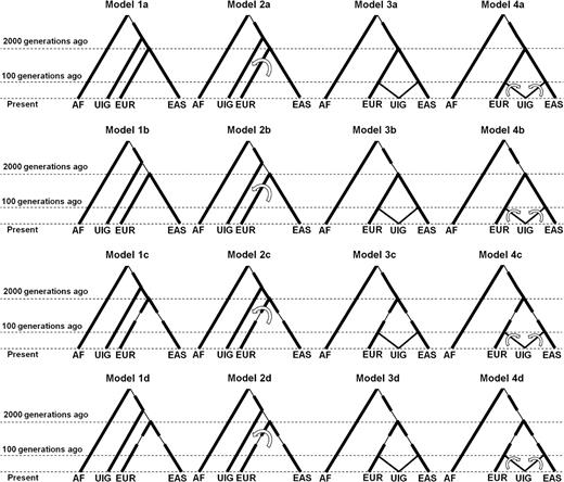
Hypothetical models for the history of UIGs. Model 1 was constructed according to H1 by assuming there is no subsequent gene flow after initial population split. Model 2 is an extension of H1 by assuming subsequent gene flow from EAS and EUR to UIG gene pool. Model 3 was constructed according to H2 by assuming that UIG was formed by single “pulse” of admixture event without subsequent gene flow after initial population admixture. Model 4 is an extension of H2 assuming additional subsequent CGF from EAS and EUR to UIG gene pool. In addition to these four primary models, a series of submodels (a–d) for each primary model were also constructed by implementing potentially possible bottleneck events.
We performed extensive forward-time computer simulations to explore all models with a diverse range of parameters. For all models, a most recent common ancestor (MRCA) population with effective population size (Ne) 10,000 was created from 120 YRI chromosomes based on 20,177 SNPs on chromosome 21, so that all chromosomes of MRCA are different but allele frequencies of MRCA mimic those of YRI. Recombination was introduced by assuming 1 cM = 1 Mb. After 1,000 generations African (AF) population and the MRCA of non-African populations diverged. AF evolved additional 5,000 generations to present with constant Ne of 10,000.
For all models, Ne for MRCA of non-African populations was set to 3,000–5,000; Ne for UIG was set to 3,000–5,000; Ne for both EAS and EUR was set to 2,000–3,000 (Tenesa et al. 2007). MRCA of non-African populations experienced no bottleneck in primary models (Model 1–Model 4) but experienced a bottleneck event during which Ne reduced to 500–2,000 with a duration of one generation. Considering the empirical recombination rate observed in chromosome 21, we assumed that 1 cM = 500 kb for all models. A recombination rate of 1 cM = 1 Mb was also assumed but no significant difference was observed. The other parameters used for each of the models are presented in table 1.
Parameters Used in Forward-Time Simulations
| Ne during Bottleneck | Admixture Proportion (%)a | Gene Flow (Effective Donors per Generation)b | Duration of Gene Flow (Generation) | |||||
| Models | EUR & EASc | EURd | EASe | EUR | EAS | EUR | EAS | |
| Model 1 | N | N | N | — | — | — | — | — |
| Model 1a | N | N | N | — | — | — | — | — |
| Model 1b | 500–1,000 | N | N | — | — | — | — | — |
| Model 1c | N | 100–300 | 100–300 | — | — | — | — | — |
| Model 1d | 500–1,000 | 100–300 | 100–300 | — | — | — | — | — |
| Model 2 | N | N | N | — | — | 2 | 1–2 | 2,000 |
| Model 2a | N | N | N | — | — | 2 | 1–2 | 2,000 |
| Model 2b | 500–1,000 | N | N | — | — | 2 | 1–2 | 2,000 |
| Model 2c | N | 100–300 | 100–300 | — | — | 2 | 1–2 | 2,000 |
| Model 2d | 500–1,000 | 100–300 | 100–300 | — | — | 2 | 1–2 | 2,000 |
| Model 3 | N | N | N | 50–60 | 50–40 | — | — | — |
| Model 3a | N | N | N | 50–60 | 50–40 | — | — | — |
| Model 3b | 500–1,000 | N | N | 50–60 | 50–40 | — | — | — |
| Model 3c | N | 100–300 | 100–300 | 50–60 | 50–40 | — | — | — |
| Model 3d | 500–1,000 | 100–300 | 100–300 | 50–60 | 50–40 | — | — | — |
| Model 4 | N | N | N | 50–60 | 50–40 | 46–35 | 26–35 | 100 |
| Model 4a | N | N | N | 50–60 | 50–40 | 46–35 | 26–35 | 100 |
| Model 4b | 500–1,000 | N | N | 50–60 | 50–40 | 46–35 | 26–35 | 100 |
| Model 4c | N | 100–300 | 100–300 | 50–60 | 50–40 | 46–35 | 26–35 | 100 |
| Model 4d | 500–1,000 | 100–300 | 100–300 | 50–60 | 50–40 | 46–35 | 26–35 | 100 |
Ancestry contribution of EUR ranges from 50% to 60%, whereas that of EAS ranges from 50% to 40% so that in each single simulation the admixture proportions summed to 100% (see Materials and Methods for details).
Gene flow was simulated under the CGF model (see Materials and Methods for details).
Bottleneck shared by EUR and EAS before they diverged; Ne of 500, 600, … 1,000 were simulated; N denotes no bottleneck was simulated.
Bottleneck occurred in EUR after the divergence of EUR and EAS, Ne of 100, 200, and 300 were simulated; N denotes no bottleneck was simulated.
Bottleneck occurred in EAS after the divergence of EUR and EAS, Ne of 100, 200, and 300 were simulated; N denotes no bottleneck was simulated.
For population admixture, we performed simulations under both hybrid-isolation (HI) model and CGF model (Long 1991) (supplementary fig. S2, Supplementary Material online). Under the HI model, UIG received ancestries of given proportions from EAS and EUR in one single generation. In Models 3 and 4 as well as their submodels (a–d), UIG was generated by population admixture, ancestry contribution from EUR ranges from 50% to 60%, whereas that from EAS ranges from 50% to 40%, so that in each single simulation the admixture proportions summed to 100%. For example, if contribution from EUR was 60%, the contribution from EAS was 40% (= 100–60%). Under the CGF model, UIG received ancestries from EAS and EUR continuously in each generation. Given the total contribution proportion and gene flow duration, the effective number of immigrants per generation can be calculated using α = 1 − (m1)1/t (supplementary fig. S2, Supplementary Material online), where α is the proportion of the effective number of immigrants per generation, m1 is the ancestry contribution proportion from the other parental population, t is the time in generation since admixture occurred. For instance, if the total ancestry contribution from EAS is 40% and from EUR is 60% during the last 2,000 generations, the effective number of EUR immigrants per generation is about 2. If the admixture occurred 100 generations ago, the effective number of EUR immigrants per generation is about 46 (table 1).
Results
Comparison of Haplotype Diversity in UIG and Other Populations
A high level of haplotype diversity is expected either in an ancient population or in an admixture population with divergent ancestries. To investigate the haplotype diversity in UIG, we calculated HHe in UIG and other four populations, namely, YRI, CEU, and CHB representing general populations and AfA representing a typical admixture population, in each distance bin (5–500 kb) based on the estimated haplotype data of 20,177 SNPs (table 2). Only results of 5–200 kb are shown because haplotype heterozygosity in all populations approaches 1 in the bins of 200 kb or larger. As expected, population with known African ancestry (AfA) shows substantially larger HHe than non-African populations (one-tailed t-test, P = 0.0003). In addition, AfA shows larger HHe than both CEU (P = 0.0007) and YRI (P = 0.01), which could be taken as its representatives of parental populations (Parra et al. 1998; Pfaff et al. 2001; Xu et al. 2007), indicating that admixture populations have a higher level of HHe than their parental populations. The increased HHe in UIG, compared with CEU (P = 0.001) and CHB (P = 0.0006), is compatible with the scenario of population admixture. However, this pattern could also be explained by a scenario that UIG is more ancient than CEU and CHB, that is, more recombination events accumulated in UIG genomes due to longer history. We therefore further conducted HSAs to investigate which scenario is more compatible with the observed data.
Haplotype Diversity in Five Populations
| CHB | UIG | CEU | AfA | YRI | |
| 5 kb | 0.505 | 0.546 | 0.530 | 0.619 | 0.597 |
| 10 kb | 0.605 | 0.651 | 0.633 | 0.758 | 0.738 |
| 20 kb | 0.691 | 0.735 | 0.716 | 0.856 | 0.843 |
| 30 kb | 0.750 | 0.790 | 0.773 | 0.902 | 0.891 |
| 40 kb | 0.786 | 0.823 | 0.807 | 0.926 | 0.919 |
| 50 kb | 0.819 | 0.850 | 0.836 | 0.942 | 0.937 |
| 100 kb | 0.908 | 0.925 | 0.917 | 0.976 | 0.975 |
| 200 kb | 0.965 | 0.970 | 0.969 | 0.987 | 0.988 |
| 500 kb | 0.988 | 0.987 | 0.990 | 0.990 | 0.992 |
| Mean | 0.780 | 0.809 | 0.797 | 0.884 | 0.875 |
| SD | 0.162 | 0.147 | 0.153 | 0.124 | 0.132 |
HS Pattern in Empirical Data
HSAs were conducted in the framework of a three-population comparison (see Materials and Methods). As shown in figure 2A, haplotypes of UIG were identified as four categories compared with CHB and CEU, that is, private in UIG (UIG), shared with CHB only (UIG–CHB), shared with CEU only (UIG–CEU), and shared with all three populations (UIG–CHB–CEU). HS percentage was calculated without considering frequencies of distinct haplotypes. In the bins up to 40 kb, UIG has less than 2% of private haplotypes (defined by at least 20 SNPs), whereas both CHB (fig. 2B) and CEU (fig. 2C) have more than 7% of private haplotypes. Even in the 200-kb bin where haplotype heterozygosity in all populations approach 1, UIG has less than 5% of private haplotypes, whereas both CHB and CEU have more than 18% of private haplotypes. When haplotype frequency was considered, this pattern still held. In the 200-kb bin, UIG has less than 2% of private haplotypes (supplementary fig. S3A, Supplementary Material online), whereas both CHB (supplementary fig. S3B, Supplementary Material online) and CEU (supplementary fig. S3C, Supplementary Material online) have more than 20% of private haplotypes. This pattern was further confirmed in another Uygur population sample (supplementary fig. S4A and Supplementary Data, Supplementary Material online) and a Hazara population sample (supplementary fig. S4B and Supplementary Data, Supplementary Material online) using HGDP data (see Materials and Methods), where both Uygur and Hazara have only about 3% of private haplotypes in 200-kb bins. Intuitively, this pattern contradicts the expectation of the hypothesis that UIG are the donors that should be more ancient than CHB and CEU so that it should have had accumulated much more private haplotypes because population divergences occurred 40 kya (Cavalli-Sforza and Feldman 2003).
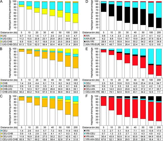
Partitions of the gene pool of each population by HSA). Haplotypes in population A were identified by HSA as four classes: 1) shared with all the three populations; 2) shared with population B only; 3) shared with population C only; and 4) private in population A. (A) UIG; (B) CHB; (C) CEU; (D) AfA; (E) CEU; and (F) YRI. HS proportions were obtained by sampling 80 chromosomes 100 times without replacement and calculated without taking into account the frequencies of distinct haplotypes.
The observed HS pattern is more compatible with a scenario of admixture where UIG are recipients with ancestry contribution from both EAS and EUR. Indeed, a typical recent admixture population, AfA does show asimilar pattern. When compared with its representatives of parental populations (YRI and CEU), AfA showed less than 5% of private haplotypes in distance bins up to 200 kb (fig. 2D, supplementary fig. S3D, Supplementary Material online), whereas CEU showed 54.7% (fig. 2E) or 53.3% (supplementary fig. S3E, Supplementary Material online) of private haplotypes and YRI showed 17.0% (fig. 2F) or 20.1% (supplementary fig. S3F, Supplementary Material online) of private haplotypes.
Therefore, it seems that a scenario of population admixture fits the observed HS pattern in UIG better. Interestingly, if admixture scenario was assumed, admixture proportion of UIG can be simply calculated from the ratio of HS percentages of UIG–CHB and that of UIG–CEU was 44%:56% (EAS:EUR) without considering haplotype frequency, or 40%:60% when haplotype frequency was considered. This estimation is very close to the result in our previous studies (Xu et al. 2008; Xu and Jin 2008) based on STRUCTURE (Pritchard et al. 2000; Falush et al. 2003) analyses.
Although the observed data supported the H2 better than the H1, we could not rule out completely the possibility that UIG was an ancient population from which EAS and EUR were derived, and its extant gene pool could be composed of ancient haplotypes as well as those received from EAS and EUR through much more recent gene flow. We next conducted extensive forward-time simulation studies to examine the haplotype-sharing pattern in various models constructed based on the two hypotheses.
Forward-Time Simulation Studies: Comparison of HS Pattern in Simulated Data and Empirical Data
To test whether the null hypothesis (UIG are donors) or the alternative hypothesis (UIG are recipients) is supported by the observed HS pattern, we constructed 20 models in total (supplementary fig. S1, Supplementary Material online, fig. 1) and performed hundreds of forward-time simulation studies with various parameters (table 1) with two replicates for each parameter setting.
Haplotype data of UIG, EAS, and EUR were collected at the end of each simulation. HSAs were conducted using simulated data and the results were compared with those observed. It is interesting that the bottleneck events do not affect the HS pattern in simulated data, that is, for models under the same assumptions, levels of UIG private haplotypes do not change alone with bottleneck size or with effective population size (fig. 3). Different assumptions for recombination rates, 1 cM = 500 kb and 1 cM = 1 Mb, did not affect the HS pattern either (supplementary fig. S5, Supplementary Material online).
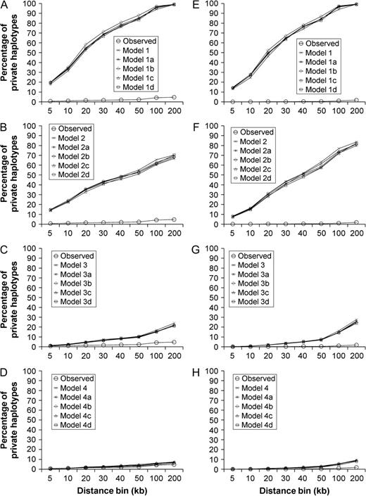
Comparison of percentage of UIG private haplotypes in empirical data and simulated data under different models. Haplotype data were simulated under four primary models, that is, Models 1–4 and their submodels (a–d) as described in figure 1. HSAs were performed in simulated data considering haplotype only (A–D) and considering both type and frequency (E–H). Percentage of private haplotypes calculated from empirical data (Observed) was also shown in each plot.
However, different models did show different HS results (figs. 3 and 4, supplementary tables S1–Supplementary Data, Supplementary Material online). Model 1 showed an extremely high level (>99%) of UIG private haplotypes in 200-kb bins, whether haplotype only (fig. 3A) or both type and frequency (fig. 3E) were considered. Model 2 showed also a high level (73% ∼ 84%) of UIG private haplotypes (fig. 3B and F), although slightly lower than Model 1. So both Models 1 and 2 contradicted with the empirical observation that UIG showed less than 5% of private haplotypes in the bins of the same sizes. Model 3 showed a level (21–28%) of UIG private haplotypes that was much closer to but still significantly higher than that observed in empirical data (fig. 3C and G). In contrast, Model 4 showed almost the same level (6–9%) of UIG private haplotypes as that observed in empirical data (fig. 3D and H). Although we focus on the HS pattern of UIG, we also conducted HSAs on other simulated populations, that is, EUR (supplementary fig. S8, Supplementary Material online) and EAS (supplementary fig. S9, Supplementary Material online). We noted that differences exist between observed and simulated data. For example, there are about 1–9% of haplotypes shared by EUR and EAS in empirical data, whereas in Models 2–4, slightly less haplotypes shared by EUR and EAS in simulated data. The difference was likely due to potential (but magnitude is unknown) gene flow between EUR and EAS that was not modeled in our simulation studies. Furthermore, we also ran simulations and HSAs using genetic map (cM) of markers obtained from the HapMap project (http://www.hapmap.org/downloads/index.html.en (to obtain genotypes of JPT, CHB, CEU, and YRI; supplementary fig. S10, Supplementary Material online). We found that different maps result in very little difference and do not alter the overall pattern.
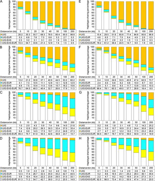
HSAs of simulated data. HSAs were performed in simulated data considering haplotype only (A–D) and considering both type and frequency (E–H). Only results obtained in UIG and from Model 1a (A,E), Model 2a (B,F), Model 3a (C,G), and Model 4a (D,H) are shown. Numbers in the table below are percentages of each class of haplotypes in UIG, that is, private in UIG (UIG), sharing with EUR only (UIG–EUR), sharing with EAS only (UIG–EAS), and sharing with both EUR and EAS (UIG–EAS–EUR).
Because Model 1 corresponds to the H1 that UIG are totally donors, the significant differences of private haplotype proportions between simulated data and empirical data (one-tailed t-test, P < 2 × 10⁻⁴) indicated this hypothesis could be rejected. Model 2 corresponds to the H1 with a great compromise, that is, UIG were previously donors but later their gene pool was replaced gradually by backward gene flow from EUR and EAS during the last 2,000 generations. It was also rejected due to the incompatibility of the simulated data with the empirical observation (P < 2 × 10⁻⁴). Model 3 corresponds to the H2 that UIG are recipients, that is, UIG in its initial history received ancestry from both EUR and EAS. But the high level of UIG private haplotypes is not fully compatible with this model (P < 9 × 10⁻³). Only population admixture with additional CGF (Model 4) is compatible with the observed pattern (P > 0.05).
Discussion
In this study, we have examined the two hypotheses on the genetic origin of the UIG, a group of people in Xinjiang, which is geographically located in central Asia. Our results showed that more than 95% of UIG haplotypes could be found in either EAS or EUR, which is unexpected under the null models assuming that the UIG are donors. Simulation studies indicated that the proportion of UIG private haplotypes observed in empirical data is only expected in alternative models assuming UIG is an admixture population. Therefore, our results favor the hypothesis based on admixture model, that is, the gene pool of modern UIGs is more likely a recipient rather than a donor.
The UIG demonstrate an array of mixed anthropological features of Europeans and Asians (Ai et al. 1993). Our previous studies indicated that UIG received ancestry from both EAS and EUR, with ancestry contribution of 40%:60% (EAS:EUR) estimated from chromosome 21 (Xu et al. 2008), and 48%:52% estimated from 22 autosomes (Xu and Jin 2008). Interestingly, if admixture scenario was assumed, admixture proportion of UIG estimated from HSA was 44%:56% (EAS:EUR) without considering haplotype frequency, or 40%:60% when haplotype frequency was considered. Therefore, this estimation is very close or even identical to the result in our previous studies (Xu et al. 2008; Xu and Jin 2008) based on STRUCTURE (Pritchard et al. 2000; Falush et al. 2003) analyses, indicating the gene pool of modern UIG could be represented by EUR and EAS ancestries. Although UIG could be a limited representative of the entire central Asian populations or even an exception, our results provide new insight for genetic history studies of human populations; if central Asian populations are more comprehensively studied in the near future and show the similar HS pattern as UIG. It should prompt a reexamination of hypotheses on the “central route” model.
It is a challenge to distinguish an ancient population from an admixed one based on modern genetic data only. It is even harder to precisely reconstruct those events that occurred in history of which the signals have been eroded by later ones. If the extent of recent gene flow is high enough, ancient haplotypes would have been replaced by immigrant ones and leave weak or no signal of ancient components in modern genomes. Our methods rely on the relative magnitude of HS among populations, which was observed in modern data thus reflect the consequences of the interplay of more complex historical events. In particular, we did not consider complex recombination models and fine-scale variations of recombination rates across chromosome in this study. In addition, haplotype analyses in this study were based on inferred haplotype data using statistical and population genetic method (Stephens et al. 2001; Scheet and Stephens 2006). Although switch errors, where a segment of the maternal haplotype is incorrectly joined to the paternal, are almost inevitable when haplotypes are inferred from genotype data of unrelated individuals, we showed in a previous study (Xu et al. 2008) that switch errors have a limited influence on the downstream analysis at the chromosome level, especially, our inferences in this study relies on the overall pattern rather than local details. Furthermore, simulation studies showed that complex recombination model, higher recombination rate, and switch errors more likely enlarge rather than reduce the difference of the HS pattern between populations (data not shown), which, if it exists widely, would have inclined the results in favor of the null hypothesis (Models 1 and 2). Therefore, in the current study, our method is conservative to the rejection of the null hypothesis.
Although we explored a huge number of combinations of models and parameters (fig. 1 and table 1), there may be still some other scenarios that we have missed; especially those scenarios and population parameters beyond our current knowledge that are mainly obtained from previous studies (Eller 2002; Cavalli-Sforza and Feldman 2003; Tenesa et al. 2007). It is still potentially possible that UIG was, although evidence is lacking, more ancient to both or either of EUR and EAS. However, even in that case, the gene pool of UIG could have been almost totally replaced during some time in history; therefore, the modern gene pool of UIG is essentially an admixture. Because there are only two central Asian populations investigated, more central Asian populations need to be examined to shed light on the human migration history involving that part of the world.
We are grateful to many people from L.J.’s laboratory and Chinese National Human Genome Center at Shanghai for their help in collecting samples. This work was supported by grants from the National Outstanding Youth Science Foundation of China (30625016), National Science Foundation of China (30890034), and 863 Program (2007AA02Z312). L.J. was also supported by Shanghai Leading Academic Discipline Project (B111) and the Center for Evolutionary Biology. S.X. was also supported by the Knowledge Innovation Program of Shanghai Institutes for Biological Sciences, Chinese Academy of Sciences (2008KIP311).
References
Author notes
Naoko Takezaki, Associate Editor
