


Abstract
The least trimmed squares (LTS) estimator is a popular robust regression estimator. It finds a subsample of h ‘good’ observations among n observations and applies least squares on that subsample. We formulate a model in which this estimator is maximum likelihood. The model has ‘outliers’ of a new type, where the outlying observations are drawn from a distribution with values outside the realized range of h ‘good’, normal observations. The LTS estimator is found to be consistent and asymptotically standard normal in the location-scale case. Consistent estimation of h is discussed. The model differs from the commonly used -contamination models and opens the door for statistical discussion on contamination schemes, new methodological developments on tests for contamination as well as inferences based on the estimated good data.
1 Introduction
The LTS estimator suggested by Rousseeuw (1984) is a popular robust regression estimator. It is defined as follows. Consider a sample with n observations, where some are thought to be ‘good’ and others are ‘outliers’. The user specifies that there are h ‘good’ observations. The LTS estimator finds the h sub-sample with the smallest residual sum of squares. Rousseeuw (1984) developed LTS in the tradition of Huber (1964) and Hampel (1971), who were instrumental in formalizing robust statistics. Huber suggested a framework of i.i.d. errors from an -contaminated normal distribution. Hampel formalized robustness and breakdown points. The present work, with its focus on maximum likelihood, deviates from this tradition.
Specifically, we propose a model in which the LTS estimator is maximum likelihood, a new approach to robust statistics. In this model, we first draw h ‘good’ regression errors from a normal distribution. Conditionally on these ‘good’ errors, we draw ‘outlier’ errors from a distribution with support outside the range of the drawn ‘good’ errors. The model is semi-parametric, so we apply a general notion of maximum likelihood. We provide an asymptotic theory for a location-scale model and find that the LTS estimator is -consistent and asymptotically standard normal. More than 50% contamination can be allowed under mild regularity conditions on the distribution function for the ‘outliers’. Interestingly, the associated scale estimator does not require a consistency factor. In practice, h is typically unknown. We suggest a consistent estimator for the proportion of ‘good’ observations, .
The approach of asking in which model the LTS estimator is maximum likelihood is similar to that taken by Gauss in 1809 (Hald, 2007, Section 5.5, 7.2). In the terminology of Fisher (1922), Gauss asked in which continuous i.i.d. location model is the arithmetic mean the maximum-likelihood estimator and found the answer to be the normal model. Maximum likelihood often brings a host of attractive features. The model provides interpretation and reveals the circumstances under which an estimator works well in terms of nice distributional results and optimality properties. Further, we have a framework for testing the goodness-of-fit, which leads to the possibility of first refuting and then improving a model.
To take advantage of these attractive features of the likelihood framework, we follow Gauss and suggest a model in which the LTS estimator is maximum likelihood. The model is distinctive in that the errors are not i.i.d. Rather, the h ‘good’ errors are i.i.d. normal, whereas the ‘outlier’ errors are i.i.d., conditionally on the ‘good’ errors, with distributions assigning zero probability to the realized range of the ‘good’ errors. When , we have a standard i.i.d. normal model, just as the LTS estimator reduces to the ordinary least squares (OLS) estimator. The model is semi-parametric, so we use an extension of traditional likelihoods, in which we compare pairs of probability measures (Kiefer & Wolfowitz, 1956) and consider probabilities of small hyper-cubes including the data point (Fisher, 1922; Scholz, 1980).
In practice, it is of considerable interest to develop a theory for inference for LTS. Within a framework of i.i.d. -contaminated errors, the asymptotic theory depends on the contamination distribution and the scale estimator requires a consistency correction (Butler, 1982; Čížek, 2005; Croux & Rousseeuw, 1992; Rousseeuw, 1984; Víšek, 2006). Since the contamination distribution is unknown in practice, inference is typically done using the asymptotic distribution of the LTS estimator derived as if there is no contamination. This seems fine for an infinitesimal deviation from the central normal model (Huber & Ronchetti, 2009, Section 12). However, these approaches would lead to invalid inference in case of stronger contamination—see Section 7.1. Within the present framework, the asymptotic theory is simpler. Specifically, we derive the asymptotic properties of the LTS estimator for a location-scale version of the presented model and find that the LTS estimator has the same asymptotic theory as the infeasible OLS estimator computed from the ‘good’ data, when it is known which data are ‘good’. As the asymptotic distribution does not depend on the contamination distribution, inference is much simpler.
In regression, a major concern is that the OLS estimator may be very sensitive to inclusion or omission of particular data points, referred to as ‘bad’ leverage points. LTS provides one of the first high-breakdown point estimators suggested for regression that also avoids the problem of ‘bad’ leverage. The presented model allows ‘bad’ leverage points.
Another key feature of the LTS model presented here is a separation of ‘good’ and ‘outlying’ errors, where the ‘outliers’ are placed outside the realized range of the ‘good’, normal observations. This way, the asymptotic error in estimating the set of ‘good’ observations is so small that it does not influence the asymptotic distribution of the LTS estimator. This throws light on the discussion regarding estimators’ ability to separate overlapping populations of ‘good’ and ‘outlying’ observations (Doornik, 2016; Riani et al., 2014).
LTS is widely used in its own right and often as a starting point for algorithms such as the MM estimator (Yohai, 1987) and the Forward Search (Atkinson et al., 2010). Many variants of LTS have been developed: nonlinear regression in time series (Čížek, 2005), algorithms for fraud detection (Rousseeuw et al., 2019) and sparse regression (Alfons et al., 2013).
In all cases, the practitioner must choose h, the number of ‘good’ observations. In our reading, this remains a major issue in robust statistics. We propose a consistent estimator for the proportion of ‘good’ observations, , in a location-scale model and study its finite sample properties by simulation. We apply it in the empirical example in Section 8.
The least median of squares (LMS) estimator, also suggested by Rousseeuw (1984), is closely related to LTS. The LMS estimator seemed numerically more attractive than LTS until the advent of the fast LTS approximation to LTS (Rousseeuw & van Driessen, 2000). Nonetheless, LMS remains of considerable interest. Replacing the normal distribution in the LTS model with a uniform distribution gives a model in which LMS is maximum likelihood. In the Online supplementary material, we show that the LMS estimator is h-consistent and asymptotically Laplace in the location-scale case. This is at odds with the slow consistency rate found in the context of i.i.d. models.
We start by presenting the LTS estimator in Section 2. The LTS regression model is given in Section 3. The general maximum likelihood concept and its application to LTS are presented in Section 4 with details in Appendix A. Section 5 presents an asymptotic theory for LTS in the location-scale case with proofs in Appendix B. Estimation of h is discussed in Section 6. Monte Carlo simulations are presented in Section 7. An empirical illustration is given in Section 8.
In a supplement, the LMS estimator is analysed and detailed derivations of some identities in the LTS proof are given. All codes for simulations and empirical illustration are available from https://users.ox.ac.uk/˜nuff0078/Discuss and as supplementary files to the paper.
Notation: Vectors are column vectors. The transpose of a vector v is denoted .
2 The LTS estimator
The available data are a scalar and a p-vector of regressors for . We consider a regression equation with regression parameter β and scale σ.
The least trimmed squares (LTS) estimator suggested by Rousseeuw (1984) is defined as follows. Given a value of β, the residuals are . The ordered squared residuals are denoted . The user chooses an integer . Given that choice, the sum of the h smallest residual squares is obtained. Minimizing over β gives the LTS estimator
The LTS minimization classifies the observations as ‘good’ or ‘outliers’. The set of indices of the h ‘good’ observations is an h-subset of . We let denote the set of indices i of the estimated ‘good’ observations satisfying . Rousseeuw and van Driessen (2000) point out that is a minimizer over least-squares estimators, that is , where
In the model proposed below, the maximum-likelihood estimator for the scale is the residual variance of the estimated ‘good’ observations
We show the consistency of in the location-scale case. The problem of estimating the scale is intricately linked to the choice of model for the innovations . Previously, Croux and Rousseeuw (1992) considered in the context of a regression model with i.i.d. innovations with distribution function . For that model, they found that should be divided by a consistency factor defined as the conditional variance of given that . In practice, is unknown, so the normal distribution is often chosen for the consistency factor.
3 The LTS regression model
We formulate the LTS model where h ‘good’ errors are assumed i.i.d. normal, while ‘outliers’ are located outside the realized range of the ‘good’ errors. This differs from the -contaminated normal model of Huber (1964), where i.i.d. errors are normal with probability and otherwise drawn from a contamination distribution. The supports of the normal and the contamination distributions overlap in the -contamination case, whereas ‘good’ and ‘outlying’ observations are separated in the below LTS model.
LTS regression model
Consider the regression model for data with . Let be given. Let be deterministic. Let ζ be a set with h elements from .
For , let be i.i.d. distributed.
Finally, suppose is invertible for all ζ.
The ‘outlier’ distributions are parameters in the LTS model. They are constrained to be continuous at zero to avoid overlap of ‘good’ and ‘outlier’ errors. Although the regressors are deterministic in Model 3.1, randomness of can be easily accommodated by a conditional model where the set of distributions are replaced by the set of conditional distributions . The likelihood below then becomes a conditional likelihood.
The LTS model allows leverage points, since can vary with j. Informally, an observation is a ‘bad’ leverage point for the OLS estimator, if that estimator is very sensitive to inclusion or omission of that observation (Rousseeuw & Leroy, 1987, Section 1.1). An example is the star data shown in Figure 1 and used in the empirical illustration in Section 8.
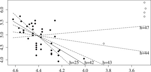
Star data and fit by LTS with different values of h. Log light intensity against log temperature. Solid dots are estimated ‘good’ observations for .
A consequence of the model is that the ‘good’ errors must have consecutive order statistics. Randomly, according to the choice of , some ‘outlier’ errors are to the left of the ‘good’ errors. The count of left ‘outlier’ errors is the random variable
Thus, the ordered errors satisfy
The set ζ collects the indices of the observations corresponding to . The difficulty in robust regression is of course that the errors are unknown. We note, that the extreme ‘good’ errors, and , are finite in any realization. As the ‘good’ errors are normal, the extremes grow at a rate for large h, see Example 5.1 below. Likewise, the ‘outlier’ errors are also finite, but located outside the realized range from to .
4 Maximum-likelihood estimation in the LTS model
The LTS model is semi-parametric. We therefore start with a general maximum likelihood concept before proceeding to analysis of the LTS model.
4.1 A general definition of maximum likelihood
Traditional parametric maximum likelihood is defined in terms of densities, which are not well-defined here. Thus, we follow the generalization proposed by Scholz (1980), which has two ingredients. First, it uses pairwise comparison of measures, as suggested by Kiefer and Wolfowitz (1956), see Johansen (1978) and Gissibl et al. (2021) for applications. This way, a dominating measure is avoided. Second, it compares probabilities of small sets that include the data point, following the informality of Fisher (1922). This way, densities are not needed. Scholz’ approach is suited to the present situation, where the candidate maximum-likelihood estimator is known and we are searching for a model.
We consider data in and can therefore simplify the approach of Scholz. Let be a family of probability measures on the Borel sets of . Given a (data) point and a distance define the hypercube , which is a Borel set.
For write if and if , where by convention .
Following Scholz, define to be equivalent at z and write if and . We get that (i) if and only if exists and equals 1; (ii) and imply (transitivity); and (iii) for all (reflexivity).
Let be a parametrized family of probability measures. Then is the -likelihood at the data point y. Further, is a maximum-likelihood estimator if for all .
The maximum-likelihood estimator is unique if for all . As for Scholz, traditional maximum likelihood is a special case. Further, the empirical distribution function is maximum-likelihood estimator in a model of i.i.d. draws from an unknown distribution.
4.2 The LTS likelihood
To obtain the -likelihood for the LTS regression Model 3.1, we find the probability that the random n-vector of observations belongs to an -cube . Throughout the argument, the regressors are kept fixed. Conditioning ‘outliers’ on ‘good’ observations, we get
For the first product for ‘good’ observations, we note that is standard normal and define and . Then, the factors of the first product in (4.1) are , which we denote .
For the second product, let and introduce
and a similar expression for , noting that if falls within the range from to . A derivation in Appendix A shows that the factors of the second product in (4.1) are . With this notation, the probability (4.1) of the -cube is
The -likelihood arises from the probability (4.2) evaluated in the data point. That is, we replace the vector z by the data vector y. We define and in a similar fashion as before. Thus, we get the -likelihood
We note that the ‘good’ errors cannot be repeated due to the assumptions that the ‘good’ observations are continuous and that the centred ‘outliers’ are continuous at zero. Thus, parameter values resulting in repetitions of the ‘good’ errors are to be ignored. As an example, suppose we have observations and we have chosen a β so that the residual takes the ordered values: 1,1,1,2,3,6,6,7,8,9. The values 1 and 6 are repetitions and cannot be ‘good’. Thus, for , we can only select ζ as the index triplet 7,8,9. All other choices are asigned a zero likelihood. The issue is essentially the same as in OLS theory, where the least-squares estimator may be useful when there are repetitions, but it cannot be maximum likelihood, as repetitions happen with probability zero under normality.
4.3 Maximum-likelihood estimation
The two products in the -likelihood (4.3) resemble a standard normal likelihood and a product of likelihoods, each with one observations from an arbitrary distribution. We will exploit those examples using profile likelihood arguments.
First, suppose are given. Then, the first product in the LTS -likelihood (4.3) is constant. In the second product, the jth factor only depends on . Since the functions vary in a product space, we maximize each factor separately. The maximum value for is unity for any and regardless of the value of . The maximum is attained for any distribution function that is continuous at zero and that rises from zero to unity over the interval from to . This set of distribution functions includes the distribution with a point mass at , which satisfies the requirement of continuity at zero, because the ‘outliers’ are separated from the ‘good’ observations. Moreover, the point mass distribution is unique in the limit for vanishing . Thus, maximizing (4.3) over gives the profile -likelihood
Second, suppose ζ is given. We argue that the unique maximum-likelihood estimator in the sense of Definition 4.2 is given by
We need to show that for all . Note that converges to a standard likelihood for a regression with normal errors. Therefore, the condition is satisfied as long as is invertible. Thus, maximizing (4.4) over gives a profile -likelihood for ζ satisfying, for ,
Third, the profile likelihood is maximized by choosing ζ so that is as small as possible. We note that the maximization is subject to the constraint that none of the ‘good’ residuals are repeated. Apart from the latter constraint, this is the LTS estimator described in (2.2). We summarize.
The LTS regression Model 3.1 has -likelihood for defined in (4.3). The maximum-likelihood estimator is found as follows. For any h-subsample ζ, let and be the least-squares estimators in (4.5). Let subject to the constraint that for , and and where . Then and .
5 Asymptotic theory for the location-scale model
We present an asymptotic theory of the LTS estimator in the special case of a location-scale model . In this model, the observations and the unknown errors have the same ranks. Thus, the ordering in (3.3) is observable and we only need to consider values of ζ corresponding to indices of observations of the form for some . Following Rousseeuw and Leroy (1987, p. 171), the LTS estimators then reduce to and , where
5.1 Sequence of data generating processes
We consider a sequence of LTS models indexed by n, so that as . In this sequence, the ‘outliers’ have a common distribution , which is continuous at zero. If the LTS estimator reduces to the full sample least-squares estimator with standard asymptotic theory. Here, we choose
where λ is the asymptotic proportion of ‘good’ observations. The parameters , vary with n, while are constant in n.
We reparametrize in terms of separate distributions for left and right ‘outliers’. Let
Thus, as is -distributed, we have that is -distributed when and is -distributed when . This leads to
This way, the ‘outliers’, for , can be constructed through a binomial experiment as follows. Draw independent variables. If the jth variable is unity then . If it is zero then . Hence, the number of left ‘outliers’ is
by the Law of Large Numbers. In summary, the sequence of data generating processes is defined by , and .
5.2 The main result
We show that the asymptotic distribution of the LTS estimator is the same as it would have been, if it had been known which observations were ‘good’. Here, we consider the case where the ‘good’ observations are normal and there are more ‘good’ observations than ‘outliers’. The result does not require any regularity conditions for the common ‘outlier’ distribution .
We expect that Theorem 5.1 would generalize to the LTS regression Model 3.1. That is, the LTS regression estimator will have the same asymptotic theory as if we knew which observations were ‘good’. The proof of such a result is, however, an open problem.
Theorem 5.1 for the LTS location-scale model differs from the known results for i.i.d. models. Butler (1982) proved a general result for the model with i.i.d. errors, showing that is asymptotically normal when the errors are symmetric with a strongly unimodal distribution. Further, the asymptotic variance involves an efficiency factor that differs from unity even in the normal case. He also gives an asymptotic theory for nonsymmetric errors. Further, Víšek (2006) analysed the regression estimator for i.i.d. errors. Johansen and Nielsen (2016b, Theorem 5) provide an asymptotic expansion of the scale estimator under normality.
A corresponding result for the LMS estimator is given in the supplement. The LMS estimator is maximum likelihood in a model where the ‘good’ observations are uniform. When there are no outliers, , the LMS estimator is a Chebychev estimator. Knight (2017) provides asymptotic analysis of Chebychev estimators in regression models. Coinciding with that theory, Online Supplementary Material, Theorem C.2 shows that the LMS estimator is super-consistent at an rate in that model, which contrasts with the well-known rate for i.i.d. models. However, Online Supplementary Material, Theorem C.2 does require regularity conditions for the ‘outliers’ to give sufficient separation from the ‘good’ observations.
5.3 Extentions of the main result
5.3.1 Nonnormal errors
We start by relaxing the normality assumption. In the spirit of OLS asymptotics, we present sufficient conditions for the ‘good’ errors: moments, symmetry, and exponential tails.
Suppose for are i.i.d. with distribution satisfying
and for ;
for and some ;
has infinite support: and ;
;
, .
The normal distribution satisfies Assumption 5.1.
For use that converges to a type I extreme value distribution when , see Leadbetter et al. (1982, Theorem 1.5.3). Here, ∼ denotes asymptotic equivalence. In particular, in probability.
For use Mill’s ratio for . Take log to see that for . We find .
Assumption 5.1 is satisfied by the Laplace distribution and the double geometric distribution with probabilities for . The latter is not in the domain of attraction of an extreme value distribution (Leadbetter et al., 1982, Theorem 1.7.13).
Assumption 5.1(iv) is not satisfied by distributions with degrees of freedom. These are in the domain of attraction of extreme value distributions of type II. Gumbel and Keeney (1950) show that converges to a nondegenerate distribution with median 1.
Consider the sequence of LTS location-scale models. Let and suppose Assumption 5.1. Then, the limiting results in Theorem 5.1 apply.
5.3.2 More ‘outliers’ than ‘good’ observations
In this section, we allow for more ‘outliers’ than ‘good’ observations. Although in the traditional breakdown point analysis there has to be more ‘good’ observations than ‘outliers’ (Rousseeuw & Leroy, 1987, Section 3.4), in practice, LTS estimators are sometimes used with more ‘outliers’ than ‘good’ observations, as in the Forward Search algorithm (Atkinson et al., 2010) for instance. We show that, within the LTS model framework, it is possible to allow for more ‘outliers’ than ‘good’ observations, but in this case, we need some regularity conditions on the ‘outliers’ to make sure the ‘good’ observations can be found.
Let the proportion of ‘good’ observations satisfy . Recall, that . is the proportion of the ‘outliers’ that are to the left. The number of ‘outliers’ to the right is . Define also the proportion of left and right ‘outliers’ relative to the number of ‘good’ observations through
Regularity conditions are needed for the ‘outlier’ distribution when or . Note that when the proportion of ‘good’ observations is and proportions of left and right ‘outliers’ are the same, so that . The following definition is convenient for analysing the empirical distribution function of the ‘outliers’, evaluated at a random quantile.
A distribution function is said to be regular, if it is twice differentiable on an open interval with so that and and the density and its derivative satisfy
and ;
If then is nondecreasing on an interval to the right of .
If then is nonincreasing on an interval to the left of .
The normal distribution is regular. Apply Mill’s ratio to see this. The exponential distribution with is also regular with and with while is decreasing as .
The following assumption requires that the ‘outlier’ distribution is regular and that the ‘outliers’ are more spread out than the ‘good’ observations.
Let . Let be -distributed and be -distributed, see (5.3).
If suppose is regular with and .
If suppose is regular with and .
Consider the sequence of LTS location-scale models. Let and suppose Assumptions 5.1, 5.2. Then, the limiting results in Theorem 5.1 apply.
Given the novelty (and perhaps at first surprising content) of Theorem 5.3, a discussion of this result and its relationship with Theorem 5.1 seems in order. Recall that Theorem 5.1 has no regularity conditions on the ‘outliers’. The result exploits that there are more than ‘good’ observations and the thin normal tails of these ‘good’ observations separate them sufficiently from the ‘outliers’. In Theorem 5.3, we allow less than ‘good’ observations but require regularity conditions on the outliers to ensure sufficient separation. More specifically, the proof of Theorem 5.3 covers two situations. First, if the proportions of left and right ‘outliers’ are equal and more than one-third of the observations are ‘good’, then , so that Assumption 5.2 is nonbinding. Second, in general, Assumption 5.2(i,ii) implies that the ‘outliers’ are spread out more than the ‘good’ observations.
This has a potential parallel with the breakdown point analysis of (Rousseeuw & Leroy, 1987, Section 3.4), which shows that for a given dataset the distribution of the LTS estimator is bounded with less than contamination of an arbitrary type. It may still be possible to obtain the same result allowing for more than contamination that satisfies regularity conditions of the type considered in Theorem 5.3, but we leave this as an open question.
5.4 The OLS estimator in the LTS model
We show that the least-squares estimator can diverge in the sequence of LTS models. This implies that the least-squares estimator is not robust within the LTS model in the sense of Hampel (1971). We assume all ‘outliers’ are to the right, so that .
6 Estimating the proportion of ‘good’ observations
The LTS regression model takes the number of good observations, h, as given. In practice, an investigator has to choose h. Estimation of h is a difficult problem, and methods for estimating h are scarce in the literature. In this section, we start by reviewing a commonly used method for choosing h and discuss its asymptotic properties. We will then propose some new methods for consistently estimating the rate of ‘good’ observations. The best of these methods is consistent at a rate. This is a slow rate and the method may be imprecise about the number h of ‘good’ observations even in large samples. Notwithstanding, to the best of our knowledge, this is the only consistent method available in the literature. Further research and improvements in this area are needed.
6.1 The index plot method
A common method for estimating h is to apply a high breakdown point LTS estimator selecting approximately observations, then compute scaled residuals for all observations and keep those observations for which the scaled residuals are less than 2.5 in absolute value. This is conveniently done using an index plot (Rousseeuw & Hubert, 1997; Rousseeuw & Leroy, 1987). More specifically, scaled residuals are plotted against the index i. Here, the consistency factor is the conditional standard deviation of given that (Croux & Rousseeuw, 1992). Bands on are displayed on the plot and observations corresponding to scaled residuals beyond these bands are declared outliers. Hence, the estimator of the number of outliers is We note that when scaling the residuals, the consistency factor is based on the assumption that all errors are i.i.d. normal.
We can analyse the asymptotic properties of the index plot method using Theorems 4, 5, 7 in Johansen and Nielsen (2016b). This will show, that in a clean, normal sample, the index plot method, asymptotically, finds outliers. In the terminology of Castle et al. (2011); Hendry and Santos (2010), γ is the asymptotic gauge of the procedure. Thus, the index plot method will on average estimate a nonzero proportion of outliers, even in uncontaminated samples.
6.2 Methods based on the LTS model
We consider methods for consistent estimation of the proportion of ‘good’ observations in the LTS model. This is a semi-parametric model selection problem where the dimension of the parameter space increases with decreasing h, since the number of functions increases when the number of ‘outliers’ increases. We consider three estimation methods. In all cases, suppose where is a lower bound chosen by the user.
Maximum likelihood. We argue that is the maximum-likelihood estimator for h. Let be the -likelihood given in (4.3) for each h. Let denote the maximum-likelihood estimator in Theorem 4.1 for each h. By (4.6), the profile likelihood for h is
We note that for all , so that is bounded uniformly in h. Thus, as whenever , so that .
An information criteria. Penalizing gives the information criteria
for a penalty f. Let be the minimizer. Then estimates the proportion of ‘good’ observations, say. Below, we argue, for the location-scale case, that is consistent if the penalty is chosen so that for increasing n, but , where . If, for instance, it is expected that more than half of the observations are ‘good’, so that , the penalty can be chosen as . The intuition is as follows.
Consider data generating processes as in Section 5.1 and let denote the number of ‘good’ observations, so that . We want to show that in the limit. Theorem 5.1 shows that is consistent for when . Thus, we consider sequences so that and argue that has a positive limit, so that the minimizer in the limit.
Suppose . In that case, one could expect that, asymptotically, the estimated set of ‘good’ observations is a subset of the good observations, so that . Further, converges to , say, the variance of a truncated normal distribution as analysed by Butler (1982). Then, , which is positive in the limit when diverges. Thus, in the limit.
Suppose . Then , where the penalty term is negative, so that must be chosen carefully. With the normal LTS model, must diverge. The reason is that, for , the estimated set of ‘good’ observations includes both ‘good’ observations and ‘outliers’. The ‘outliers’ diverge at a rate, see Example 5.1, so that must diverge at a rate. Noting that , we get . When , we have , and the term dominates when . Thus, in the limit.
Combining these arguments indicates that in the limit. Unfortunately, in simulations that are not reported here, we find that a penalty grows so slowly in n that for some specifications the consistency is only realized for extremely large samples.
Cumulant based normality test. A more useful estimator for the proportion of ‘good’ observations λ is the minimizer , say, of the normality test statistic
based on third and fourth cumulants of the estimated ‘good’ residuals. We argue that is consistent for . This is supported by a simulation study in Section 7.2.
The intuition of the consistency argument is similar to that for the information criteria. First, for , Theorem 5.1 may be extended to show that is asymptotically . For , the sample moments may converge to the moments of a truncated normal distribution, see Berenguer-Rico and Nielsen (2017). Thus, would diverge as it is normalized using the normal distribution. For , the estimated set of ‘good’ observations contains both ‘good’ and ‘outlying’ observations, so that diverges at a logarithmic rate, instead of the iterated logarithmic rate for the information criteria. A formal proof is left for future work.
7 Simulations
7.1 Inference in the location-scale model
In the location-scale model , we study the finite sample properties of tests for using four different tests statistics and six different data generating processes, which we describe below. We consider sample sizes and let .
Tests. We consider four different estimators: LTS, LMS, OLS and SLTS (scale-corrected LTS estimator). For each estimator, s say, we compute t-type statistics, , with associated asymptotic 95% quantiles .
For the OLS estimator, we have and with . The asymptotic quantile is standard normal.
For the LTS estimator, we apply the estimators and given in (5.1). By Theorem 5.2, we get that . The asymptotic quantile is standard normal.
For the LMS estimator, we apply the estimators and given in Online Supplementary Material, (C.4). Online Supplementary Material, Theorem C.2 gives that . The asymptotic quantile is standard Laplace.
Finally, SLTS uses the usual approach to LTS estimation with consistency and efficiency correction factors arising from truncation in a standard normal distribution as outlined in the end of Section 2. Let with c chosen so that , which gives . Then, we have estimators and , while . The asymptotic quantile is standard normal.
Data generating processes (DGPs). Table 1 gives an overview of the DGPs. The first three DGPs are examples of the LTS Model 3.1 and the LMS Online Supplementary Material, Model C.1. The proportion of ‘good’ observations is . The ‘good’ errors are i.i.d. normal in DGP1 and DGP2 and i.i.d. uniform in DGP3. The ‘outlier’ errors are defined as in (3.1), so that , where are i.i.d. normal and and separate ‘good’ and ‘outlying’ observations. The separators are in DGP1 and , in DGP2 and DGP3.
Data generating processes
| Model | MLE | ‘good’ error | ‘outliers’ | |
|---|---|---|---|---|
| DGP1 | LTS | LTS | ||
| DGP2 | LTS | LTS | , | |
| DGP3 | LMS | LMS | , | |
| DGP4 | -contamination | OLS | ||
| DGP5 | -contamination | — | ||
| DGP6 | -contamination | — |
| Model | MLE | ‘good’ error | ‘outliers’ | |
|---|---|---|---|---|
| DGP1 | LTS | LTS | ||
| DGP2 | LTS | LTS | , | |
| DGP3 | LMS | LMS | , | |
| DGP4 | -contamination | OLS | ||
| DGP5 | -contamination | — | ||
| DGP6 | -contamination | — |
Note. The proportion of good errors is . Columns 2 and 3 show the model and indicate which estimator is maximum likelihood. Columns 4 and 5 indicate how the ‘good’ and the ‘outlying’ errors are chosen. For DGP1 – DGP3: ‘good’ observations,‘outliers’ have is . For DGP4 – DGP6: distribution is .
The last three DGPs are examples of -contamination (Huber, 1964). We draw n observations from the distribution function , where Φ is standard normal and represents contamination. In DGP4, , giving a standard i.i.d. normal model. In DGP5 and DGP6, is and , giving symmetric and nonsymmetric mixtures, respectively.
We have different maximum-likelihood estimators for the different models. These are LTS for DGP1 and DGP2, LMS for DGP3, and OLS for DGP4. None of the considered estimators are maximum likelihood for DGP5 and DGP6.
Table 2 reports results from repetitions. The Monte Carlo standard error is 0.001.
Simulated rejection frequencies for nominal 5% tests on intercept
| n | DGP1 | 2 | 3 | 4 | 5 | 6 | DGP1 | 2 | 3 | 4 | 5 | 6 |
|---|---|---|---|---|---|---|---|---|---|---|---|---|
| OLS | LTS | |||||||||||
| 25 | 0.092 | 0.084 | 0.084 | 0.067 | 0.066 | 0.359 | 0.255 | 0.081 | 0.072 | 0.371 | 0.337 | 0.388 |
| 100 | 0.083 | 0.129 | 0.199 | 0.054 | 0.054 | 0.887 | 0.180 | 0.058 | 0.055 | 0.383 | 0.345 | 0.518 |
| 400 | 0.100 | 0.321 | 0.664 | 0.051 | 0.051 | 1.000 | 0.110 | 0.052 | 0.051 | 0.389 | 0.349 | 0.827 |
| 1600 | 0.159 | 0.745 | 0.998 | 0.050 | 0.050 | 1.000 | 0.071 | 0.050 | 0.050 | 0.390 | 0.349 | 0.998 |
| LMS | SLTS | |||||||||||
| 25 | 0.720 | 0.489 | 0.070 | 0.641 | 0.631 | 0.702 | 0.011 | 0.000 | 0.000 | 0.034 | 0.027 | 0.063 |
| 100 | 0.961 | 0.785 | 0.054 | 0.836 | 0.831 | 0.901 | 0.002 | 0.000 | 0.000 | 0.041 | 0.028 | 0.116 |
| 400 | 0.999 | 0.936 | 0.051 | 0.931 | 0.929 | 0.982 | 0.000 | 0.000 | 0.000 | 0.047 | 0.031 | 0.373 |
| 1600 | 1.000 | 0.992 | 0.050 | 0.972 | 0.971 | 0.999 | 0.000 | 0.000 | 0.000 | 0.049 | 0.032 | 0.941 |
The OLS statistic is maximum likelihood with DGP4 and performs well. It performs equally well with the symmetric, i.i.d. DGP5. For DGP1, it is slowly diverging, possibly because the absolute sample mean is diverging with n. OLS performs poorly with the nonsymmetric DGP2, DGP3, and DGP6.
The LTS statistic is maximum likelihood with DGP1 and DGP2. The asymptotic theory also applies for DGP3. The convergence is slow for DGP1, where there is no separation. The LTS statistic does not perform well with -contamination in DGP4, DGP5, and DGP6.
The LMS statistic is maximum likelihood with DGP3 and perform well with that DGP, but poorly with all other DGPs. The SLTS statistic is not maximum likelihood for any of the considered models. It is calibrated to be asymptotically unbiased for DGP4 and performs well for that model, but poorly with all other DGPs.
Overall, we see that it is a good idea to apply maximum likelihood but this does require that the model specification is checked. In particular, the LTS estimator is best in DGP1–DGP3, although with some finite sample distortion with DGP1 where ‘good’ and ‘outlying’ observations are not well-separated. The LTS estimator does not work well for the -contaminated models, where a model dependent scale correction is needed. The usual approach of using the normal scale correction as in SLTS does not work well in general. All estimators are poor for asymmetric -contamination.
7.2 h estimation
Next, we study the finite sample properties of estimating h using the cumulant-based normality test statistic in (6.2). Results are reported in Table 3, based on repetitions.
Estimating h by minimizing the statistic in (6.2)
| DGP1 | DGP2 | |||||||||||
|---|---|---|---|---|---|---|---|---|---|---|---|---|
| n | ||||||||||||
| 25 | 1.2 | 2.5 | 1.0 | 2.5 | 0.3 | 2.1 | 1.5 | 2.1 | ||||
| 100 | 9.6 | 8.6 | 3.7 | 6.0 | 0.2 | 4.3 | 1.1 | 3.0 | ||||
| 400 | 41.3 | 35.8 | 4.5 | 12.4 | 0.8 | 2.1 | ✓ | 0.8 | 2.0 | ✓ | ||
| 1600 | 92.8 | 143.1 | ✓ | 0.4 | 3.5 | ✓ | 0.8 | 2.0 | ✓ | 0.8 | 2.0 | ✓ |
| 12800 | 0.7 | 4.2 | ✓ | 0.6 | 4.4 | ✓ | 1.2 | 3.2 | ✓ | 1.3 | 3.2 | ✓ |
Note. Here, and report the simulated bias and standard deviation for , while is ticked if all simulated values of are interior to the range from 60% to 90%.
In each repetition, we compute the statistic for each h in the range from 60% to 90% of n. The estimator of h is the minimizer of over that range.
The data generating processes are DGP1 and DGP2 from above. These are examples of the LTS model, so that DGP1 has symmetric ‘outliers’ that are not separated from the ‘good’ observations, while DGP2 has asymmetric ‘outliers’ that are separated from the ‘good’ observations. For each DGP, we consider cases with 70% or 80% ‘good’ observations.
Table 3 reports three quantities for each of the DGPs. First, and are the Monte Carlo average and standard deviation of the estimation error . Further, is a binary variable, which is checked if is in the interior of the range from 60% to 90% of n for all simulations. The theory suggests that the proportion of ‘good’ observations is consistently estimated, whereas h is not consistently estimated. Thus, we would expect and to grow slower than linearly in n, but not to vanish.
For all the four set-ups, the simulations confirm that is consistent for λ. In DGP1, where there is only little separation between ‘good’ and ‘outlying’ observations, the performance differs substantially between the cases and . We do not have an explanation for this difference. Nonetheless, the estimation works much better for DGP2, with its separation between ‘good’ observations and ‘outliers’, in both cases and , matching the theoretical discussion in the above sections.
We also considered the information criteria in (6.1), but omit the results. The performance of is poor, quite possibly due to the rates involved.
8 Empirical illustrations
We provide two empirical illustrations using the stars data of Rousseeuw and Leroy (1987) and the state infant mortality data of Wooldridge (2015). Both analyses illustrate the estimation of h. The second case also illustrates inference in the LTS model. Therefore, we must determine empirically if the LTS model is appropriate. Indeed, there could be a contamination pattern that is consistent with the -contamination, with the LTS model, or with neither of those. For both illustrations, we study the source of the data to arrive at reasonable empirical models.
Throughout, we use R version 4.0.2 (R Core Team, 2020) estimating LTS using ltsReg from the Robustbase package. Before each LTS call we apply set.seed(0). R code with embedded data is available as Supplementary material.
8.1 The stars data
For this empirical illustration, we consider the data on log light intensity and log temperature for the Hertzsprung–Russell diagram of the star cluster CYG OB1 containing stars as reported by Rousseeuw and Leroy (1987, Table 2.3). Figure 1 shows a cross plot of the variables, where the log temperature axis is reversed. The majority of observations follow a steep band called the main sequence. Rousseeuw and Leroy (1987) refer to the four stars to the top right of Figure 1 as ‘outliers’.
By consulting the original source of the data in Humphreys (1978), see also (Vansina & De Grève, 1982, Appendix A), we found that the 4 stars to the right of Figure 1 are of M-type (observations 11, 20, 30, 34) and they are red supergiants. Further, the fifth star from the right is of F-type (observation 7, called 44 Cyg). The next 31 stars (1 doublet) from the right are of B-type and the remaining 11 stars (1 doublet) furthest to the left are of the O-type. The doublets are not exact doublets in Humphreys’ original data, so this in itself should not be seen as evidence against a normality assumption.
We fitted the linear model . Table 4, left panel, shows LTS estimates for different h values. For , the LTS estimator is the full sample OLS estimator. The β estimates are the ‘raw coefficients’ found by ltsReg while is computed directly from (2.3) without any consistency correction. Figure 1 shows LTS fits for selected values of h. It is seen that the fits rotate when h increases. Table 4 also reports the criterion as a function of h. It is minimized for pointing at five ‘outliers’: The four M-stars and the F-star. Figure 1 indicates estimated ‘good’ observations and ‘outliers’ with solid and open dots.
Estimates by LTS and criterion for selecting h
| Full sample | Sub sample | |||||||
|---|---|---|---|---|---|---|---|---|
| h | ||||||||
| 25 | 13.62 | 4.22 | 0.18 | 1.72 | 13.62 | 4.22 | 0.18 | 1.72 |
| 36 | 11.49 | 3.71 | 0.27 | 1.98 | 11.49 | 3.71 | 0.27 | 1.98 |
| 37 | 9.00 | 3.16 | 0.28 | 2.49 | 9.00 | 3.16 | 0.28 | 2.49 |
| 40 | 8.58 | 3.07 | 0.31 | 2.13 | 8.58 | 3.07 | 0.31 | 2.13 |
| 41 | 8.50 | 3.05 | 0.33 | 1.26 | 8.50 | 3.05 | 0.33 | 1.26 |
| 42 | 7.40 | 2.80 | 0.37 | 0.39 | 7.40 | 2.80 | 0.37 | 0.39 |
| 43 | 4.06 | 2.05 | 0.40 | 0.69 | 7.88 | 0.65 | 0.49 | 2.57 |
| 44 | 1.89 | 0.70 | 0.49 | 0.49 | 7.74 | 0.62 | 0.51 | 2.76 |
| 45 | 7.34 | 0.53 | 0.51 | 2.94 | 7.58 | 0.59 | 0.53 | 2.73 |
| 46 | 6.92 | 0.44 | 0.53 | 2.74 | 7.12 | 0.49 | 0.55 | 2.83 |
| 47 | 6.79 | 0.41 | 0.55 | 2.75 | ||||
Note. Left panel has full sample. Right panel excludes the F-type star.
The estimation of h by the statistic appears a little shaky in Table 4, left panel. The lowest value is obtained for , while the value for is nearly as low. The slope coefficients change gradually for with no obvious choice of h for . Table 4, right panel, shows corresponding results when dropping the F star from the sample. The results are the same for . We see that is now a clear minimum identifying the four M-type stars as ‘outliers’. The M stars appear to have a masking effect, where after their deletion, the F star emerges as very influential in the sense of Rousseeuw and Leroy (1987, p. 81). Perhaps for this reason, different conclusions are reached by different traditional methods. An LTS index plot points at 5 ‘outliers’, see Section 6.1, while an MM index plot (using lmrob in the R package robustbase) and LMS residuals (using lmsreg in the R package MASS) both point at 4 ‘outliers’, not detecting the F star as ‘outlying’.
Figure 2 shows kernel density plots for the scaled residuals for . The black, thin lines gives kernel densities for the full sample. The red, dashed lines gives kernel densities for the estimated ‘good’ observations. The standard normal distribution is shown with a blue, thick line. For , the red, blue, and part of the black lines coincide, which indicates the normality of the ‘good’ observations. The full sample kernel density has a probability mass in the right tail corresponding to the four giants. There is a slight discrepancy between the full sample and the ‘good’ kernel densities in the region from 2 to 4 corresponding to the F star. By construction this 43rd residual will be outside the range of the 42 ‘good’ residuals, but not by far. Kernel densities are very sensitive to the choice of kernel and bandwidth. For illustration, we chose a Gaussian kernel and bandwidth to get the best match of the red and blue curves for . With that choice, we can more clearly see discrepancies between the kernel density for the ‘good’ observations and the normal curve for , that is, for the LTS with a high breakdown point and the OLS estimator, respectively.
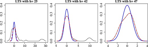
Scaled LTS residuals for . Kernel densities for all residuals (thin) and for ‘good’ residuals (dashed) with fitted standard normal density (thick).
8.2 State infant mortality rates
We consider 1990 data for the United States on infant mortality rates by state, including Washington DC, which has a particularly high infant mortality rate (Wooldridge, 2015, p. 299). The data are available as infmrt in the R package wooldridge and are taken from U.S. Bureau of the Census (1994). We analyse two models.
The first model follows Wooldridge. It is a linear regression of the number of deaths within the first year per 1,000 live births, infmort, on the log of per capita income, lpcinc, the log of physicians per 100,000 members of the civilian population, lphysic, and the log of population in thousands, lpopul. In Figure 3, the graph using circle symbols shows the cumulant-based criteria as function of h. The OLS regression is obtained for and has a rather large value of —notice the gap in the -axis—indicating that the full sample model is mis-specified. Choosing would lead to one ‘outlier’, which is Washington DC. However, the function is minimized at indicating six ‘outliers’: Delaware, Washington DC, Georgia, Texas, California, and Alaska (U.S. Bureau of the Census, 1994, Table 123). The interpretation is not obvious and could be due to a missing regressor.

State infant mortality rates. criterion as function of h. Model for infmrt shown with circles. Model for infmrt shown with squares.
The second model differes in two respects. It applies logarithms to the regressand to stabilize rates close to zero as well as for Washington DC. It also includes a regressor for the log proportion of black people in the population, lblack (U.S. Bureau of the Census, 1992, Table 255), since infant mortality is quite different for white and black infants in most states (U.S. Bureau of the Census, 1994, Table 123). In Figure 3, the graph using square symbols shows versus h for this model. The minimizer is with Washington DC as the ‘outlier’. The minimum of is small compared with a distribution, so no evidence against the LTS model. We note that the function is also quite low for h in the left side of the plot, albeit not as low as for . The estimated LTS model for is
The standard errors are the usual OLS standard errors as the LTS model appears to apply. We conclude that the variables lpcinc and lpopul are not significant.
Changing the regressand to be measured on the original scale introduces a second ‘outlier’, South Dakota, which has one of the lowest infant mortality rates for the black population.
9 Concluding remarks
Estimating the proportion of ‘good’ observations. We consider a few issues regarding the estimation of h and the adequacy of the model in the two empirical examples.
First, the sample sizes, and , are rather small. The results in Section 6.2 indicate that the estimation of based on the criterion is consistent, hence, it may be imprecise in small samples.
Second, the results in Section 6.2 focus on the location-scale LTS model. The empirical illustrations above consider models with regressors. We believe the estimation of λ based on the criterion extends to a well-specified multiple LTS regression model. However, as pointed out in Section 8.2, the omission of regressors could interfere with the estimation of λ. This aspect needs further investigation.
Third, the results in Section 6.2 refer to the LTS model, where, once ‘outliers’ have been removed, the remaining ‘good’ observations look normal. In practice, the adequacy of the model in a given data set has to be studied. A formal testing procedure is not yet available for the present model. Estimating λ by the criterion is unlikely to be consistent in a model where ‘outliers’ are generated by -contamination.
Fourth, notwithstanding the above issues, the suggested procedure for selecting h seems to work well in the two empirical illustrations in this section and helped in finding satisfactory LTS models for the data.
Other models of the LTS type. New models and estimators can be generated by replacing the normal assumption in the LTS models with some other distribution. For instance, the uniform leads to the least median of squares (LMS) estimator analysed in Online Supplementary Material, Appendix C, while the Laplace distribution leads to the least trimmed sum of absolute deviations (LTA) estimator (Dodge & Jurečková, 2000; Hawkins & Olive, 1999; Hössjer, 1994, Section 2.7). Ron Butler has suggested to us that the approach in this paper could also be applied to the minimum covariance determinant (MCD) estimator for multivariate location and scale (Butler et al., 1993; Rousseeuw, 1985).
Alternative models for ‘outliers’. The maximum likelihood argument in Section 4 would also work if the ‘outlier’ errors rather than have distribution . The analysis would be related to the trimmed likelihood argument of Gallegos and Ritter (2009). However, the resulting LTS estimator would have less attractive asymptotic properties in that model compared to those derived in this paper.
Inference requires a model for both ‘good’ and ‘outlying’ observations. In the presented theory, the ‘good’ and the ‘outlying’ observations are separated. The traditional approach, as advocated by Huber (1964), is to consider mixture distributions formed by mixing a reference distribution with a contamination distribution. Any subsequent inference on the regression parameter β would require a specific formulation of the -contaminated distribution. This is a nontrivial practical problem. Instead, there has been a focus on showing that the bias of estimators is bounded under contamination (Huber & Ronchetti, 2009, Section 4) while inference is conducted using the asymptotic distribution that assumes all observations are i.i.d. normal, implying that the ‘good’ observations are truncated normal. This gives a different distribution theory for inference compared with the one presented here and simulations in Section 7.1 indicate that this will not control size in general. It is therefore of interest to formulate models allowing ‘outliers’ under which consistency can be proved. The LTS model in this paper does so. The presented simulations show that the two inferential theories are really very different. In practice, LTS estimation should therefore be evaluated in the context of a particular model and inference should be conducted accordingly.
Alternative estimators of h. We have proposed consistent estimators for , but it would be useful to investigate their performance further. In a regression context, it may be worth considering the Forward Search algorithm (Atkinson et al., 2010). Omitted regressors and ‘outliers’ may confound each other, so a simultaneous search over these may be useful as in the Autometrics algorithm (Castle et al., 2021; Hendry & Doornik, 2014). Some asymptotic theory for these algorithms are provided in Johansen and Nielsen (2016a, 2016b).
Misspecification tests can be developed for the present model. The asymptotic theory developed here shows that standard normality tests can be applied to the set of estimated ‘good’ observations. Other tests could also be investigated, in particular those that are concerned with functional form or omission of regressors.
More ‘outliers’ than ‘good’ observations. This is allowed in the LTS model and supported by the asymptotic analysis under regularity conditions for the ‘outliers’. This lends some support to the practice of starting the Forward Search algorithm by an LTS estimator for fewer than half of the observations (Atkinson et al., 2010). Whether it makes more sense to model the ‘outliers’ or the ‘good’ observations as normally distributed in this situation must rest on a careful consideration of the data and the substantive context.
Acknowledgments
Comments from R. Butler, Y. Gao, O. Hao, C. Henning, referees, and the associate editors are gratefully acknowledged.
Data availability
All the data that we use are publicly available; the precise sources are cited in the article. The source code files in R available as Supplementary material.
Supplementary material
Supplementary material are available at Journal of the Royal Statistical Society: Series B online.
Appendix A. Derivation of the LTS likelihood
We prove that
First, we prove that , where the dot indicates the conditioning set. Since and , we have that .
Recall that the ‘outlier’ errors are see (3.1) and since . Further, has distribution function , which is continuous at zero. As a consequence, and . Thus, for .
Let , where and .
By (3.1), we have , so that can be written as . Hence,
Similarly, by (3.1). If , then the intersection is empty. If instead , then, the intersection is the set . Hence,
Note also that if , then . And, if , then . In combination, we have
Recall the notation . We then get .
Second, similarly, . Combining, the desired result follows.
Appendix B. Proofs of asymptotic theory for the LTS model
We start with some preliminary extreme value results, which then allows analysis of the case with more ‘good’ observations than ‘outliers’. Then some results on empirical processes follows, which are needed for the general case.
B.1 Extreme values
For a distribution function define the quantile function .
Suppose for . Let . Then .
Let a small be given. Then a finite exists to that . We show where . Applying , we get . By the Law of Large Numbers, . Hence, if then for large n. Since , we have . Here, by construction. Moreover, where for large n since by assumption. Thus, . □
Suppose are i.i.d. with for some . Then for any .
We show for any . Write . Boole’s inequality gives . Markov’s inequality gives , which vanishes for . □
B.2 Some initial properties of the LTS estimator
We consider the LTS estimator under the sequence of data generating processes defined in Section 5.1. The main challenge is to show that is close to the -distributed variable . In the following lemmas, we condition on the sequence , so that the randomness stems from ‘good’ errors and the magnitudes of the ‘outliers’, for and for . The unconditional statements in the Theorems about are then derived as follows. If for an interval and a sequence then by the law of iterated expectations
due to the dominated converges theorem, because is bounded.
We give detailed proofs for the case , so that some of the small ‘good’ observations are considered left ‘outliers’ and some of the small right ‘outliers’ are considered ‘good’. The case is analogous, since we can multiply all observations by and relabel left and right. When considering we note that , the number of right ‘outliers’. Recall . Hence, if , then all outliers are to the left. In particular, due to the binomial construction of then . when , so that the event is a null set. Thus, when analysing it suffices to consider and .
The next lemma concerns cases where is small. We show that the LTS estimators are close to the infeasible OLS estimators for the ‘good’ observations. We note that, by Lemma B.2 and Assumption 5.1(ii) that , we can find a small so that . We write for .
Consider the LTS estimator under Assumption 5.1(ii). Let for some small defined above. Then, and are .
The next Lemma is the main ingredient to showing consistency of . It is convenient to define sequences
We note that by Assumption 5.1(iii), has a distribution function with infinite support. Hence, the extreme value diverges to infinity and . By Assumption 5.1(ii), Lemma B.2 applies, so that for some . Then, for large and η small, where .
Suppose Assumption 5.1 and let and . Then, for any , we have in probability.
1. Considerwhere. We start by finding a lower bound to . The range of interest is . As argued above . The function is concave with roots at and . Then, for with , the function has two minima, one at and the other one at . Therefore, . Thus, on the considered range.
Next, we bound uniformly in s as in (B4).
For use so that .
Thus, (B5) reduces to Since in probability and by Assumption 5.1(iv) we get that . In particular, in probability.
2. Considerwherefor anyand, see (B2). We find bounds for the terms in (B5).
First, . Write , where . In the left tail, the squared order statistics decrease with increasing index with large probability. Hence, we can bound . Bounding and we get . By Assumption 5.1(iv,v) then and for some . Then, , which reduces to .
Second, by definition.
B.3 Fewer ‘outliers’ than ‘good’ observations
First, we show that for any . It suffices to show for each η.
As discussed above, we consider the case , so that some of the small ‘good’ observations are considered left ‘outliers’ and some of the small right ‘outliers’ are considered ‘good’. The case is analogous. When considering we note that , the number of right ‘outliers’. Moreover, , since there are right ‘outliers’ and ‘outliers’ in total.
Choose and as in (B2). Since converges to a value less than unity then for large n. Thus, if we show then as desired. Now, is the minimizer of . Since , then if in probability. This follows from Lemma B.4 using Assumption 5.1.
Second, since then Lemma B.3 using Assumption 5.1(ii) shows that , are .
Third, the i.i.d. Law of Large Numbers and Central Limit Theorem using Assumption 5.1(i) show that is asymptotically normal while is consistent for . □
B.4 Marked empirical processes evaluated at quantiles
We start with some preliminary results on marked empirical processes evaluated at quantiles.
Consider random variables for and define the marked empirical distribution and its expectation, for , by
For , let . We also define the quantile function and the empirical quantiles . The first result follows from the theory of empirical quantile processes.
Suppose is regular (Definition 5.1). Then, for all ,
converges in distribution on to a Brownian bridge;
.
This is Billingsley (1968, Theorem 16.4).
Let and write the object of interest as the sum of and . These two terms are . by Csörgö (1983, Corollaries 6.2.1, 6.2.2), uniformly in ψ. □
We need the following Glivenko–Cantelli result.
Let be i.i.d. continuous, positive random variables with . Then .
We note that is nondecreasing with . Since is continuous, then for any exists a finite integer and chaining points so that .
The next result is inspired by Johansen and Nielsen (2016a, Lemma D.11).
Let . Suppose is positive, regular and for some . Then, .
Consider . Write . Lemma B.2 shows for since by assumption.
Consider . Bound , where satisfies . We must show . It suffices that for . By the Markov inequality , so that . □
B.5 More ‘outliers’ than ‘good’ observations
The next lemma is needed when there are more than half of the observations are ‘outliers’. As is not diverging, additional regularity conditions are needed to ensure that .
Suppose Assumption 5.2(i) holds. Let . Recall , from (B2). Then, conditional on , an exists so that for large n.
The errors are standard normal order statistics for and for , where is -distributed. We let .
It suffices to show that uniformly in s, since by the Law of Large Numbers using Assumption 5.1(i) applied to the sample variance of the ‘good’ errors. We consider separately the cases and .
1. Consider. In this case, is the sample variance of for . Sample variances are invariant to the location, so that . Let .
We argue, as in part 1, that . Indeed, since , then . Both bounds equal , so that we can proceed as in part 1. □
We will show that for any . It suffices to consider the case where and where as remarked in Section 5.1. We consider so that satisfies . The case was covered in the proof of Theorem 5.2. Thus, suppose .
Recall from (B2). In particular, for large n, so that . We show, that the latter probability vanishes. Note that .
We have that is the minimizer to , which is zero for . The Lemmas B.4, B.8 using Assumption 5.2(i) show that , asymptotically, has a uniform, positive lower bound on each of the intervals and . Thus, is bounded away from zero on so that .
A similar argument applies for using Assumption 5.2(ii). The limiting results for then follow as in the proof of Theorem 5.2. □
B.6 The OLS estimator in the LTS model
References
Author notes
Conflict of interest: None declared.
