


Abstract
Background. The familial recurrence risk of lymphatic filariasis (LF) is unknown. This case study aimed to evaluate the familial susceptibility to infection with Wuchereria bancrofti and to microfilaremia in a village of the Republic of Congo.
Methods. The heritability and intrafamilial correlation coefficients were assessed for both W. bancrofti infection and microfilaremia by controlling for individual risk factors, environmental influence, and household effects.
Results. Pedigree charts were constructed for 829 individuals, including 143 individuals with a diagnosis of W. bancrofti circulating filarial antigens (CFAs) and 44 who also had microfilariae (MF). There was no intrafamilial correlation regarding CFA levels. However, the presence of MF (ρ = 0.45) and microfilarial density (ρ = 0.44) were significantly correlated among parent-offspring pairs. Heritability estimates for CFA positivity and intensity were 0.23 and 0.18, respectively. Heritability estimates were high for microfilarial positivity (h2 = 0.74) and microfilarial density traits (h2 = 0.81).
Conclusions. Our study suggests that the acquisition of LF is mainly driven by environmental factors and habits and that genetic factors are moderately involved in the regulation of infection. By contrast, genetic factors play a major role in both the presence and intensity of microfilaremia.
Lymphatic filariasis (LF) affects some 120 million people and is the second leading cause of disability worldwide, with one third of those infected experiencing severe symptoms [1]. LF is mainly due to Wuchereria bancrofti and, to a lesser extent, Brugia malayi and Brugia timori. Exposure, transmission potential, environmental, parasite, host, and immune factors can play a role both in the acquisition of infection and in the biological and clinical course of the disease and can explain the variability in epidemiological patterns observed around the world.
Complex immune regulations play a role in susceptibility to LF [2, 3]. Individuals with latent infection (defined as the presence of adult worms without detectable microfilaremia) are thought to have an increased adaptive immune response, in contrast to patients with patent infection (defined as the presence of microfilariae [MF]) who have an immunosuppressive status [4]. Because the host immune system is partly controlled by genetic factors, several studies have assessed familial susceptibility to LF. Familial clustering of cases has been shown, suggesting genetic susceptibility to infection (defined as the presence of circulating filarial antigens [CFAs]), to microfilaremia [5, 6], or to lymphedema [7–9]. Gene polymorphisms associated with a microfilaremic phenotype and with hydrocele development were also identified [10–12]. However, only one study, performed in an area with subperiodic W. bancrofti endemicity, estimated the proportion of phenotypic variance due to genetic factors (heritability) and found that genetics plays a major role in infection and microfilaremic statuses [13]. Since heritability is specific to a given population and strongly depends on the role played by environmental factors, these results cannot be extrapolated to all areas of endemicity [14]. Moreover, heritability does not provide any information on individual risk (estimated by relative recurrence risk or intrafamilial correlation coefficients) [15].
The aim of the present study was to evaluate the genetic component of the familial susceptibility to infection with W. bancrofti in a village of Central Africa by controlling for a number of individual risk factors and environmental influences. Variance components analysis based on maximum likelihood procedures was used to estimate the proportion of phenotypic variation attributable to genetic effects, and patterns of familial correlations were examined for both infection and microfilaremic phenotypes among different classes of relatives (eg, parent-offspring or father-son).
METHODS
Study Population and Procedures
The study was performed in Séké Pembé (Republic of Congo), where a trial was conducted to evaluate the impact of semiannual community treatments with albendazole alone on W. bancrofti. Before the first treatment, the prevalence of filarial antigenemia was 23.9%. The study population has been previously described [16, 17]. Séké Pembé is located in a savannah area, 20 km north of Madingou, the capital town of the Bouenza division. After an exhaustive census of the population, blood samples were collected from consenting adults and assenting children aged ≥5 years, and CFA were detected using the Binax Filariasis Now Card immunochromatographic test (ICT; Alere, Scarborough, Maine) read after 10 minutes. The results were scored as 0 for tests with no visible test (T) line, 1 for tests with a weaker T line than control (C) line, 2 for tests with a T line as dark as the C line, and 3 when the T line was darker than the C line. This semiquantitative scoring allowed us to estimate the number of adult worms present in the individual [18]. ICT-positive subjects were tested for the presence of MF in night blood (2 bloods smears of 70 μL). A questionnaire was administered to collect information on the domestic and peridomestic environment (access to private latrine and use of bed nets during the previous night), and other personal activities (fishing, hunting, and sleeping outdoors in the bush) potentially related to exposure to mosquito bites. All individuals included in the analyses had no history of albendazole or ivermectin treatment.
Definition of Phenotypes
Each individual was attributed the following phenotypes: (1) infected versus noninfected (ICT+ vs ICT−), (2) microfilaremic versus amicrofilaremic (ICT+/MF+ vs ICT+/MF−), (3) intensity of infection (ICT score from 0 to 3), and (4) microfilarial density (DMF; defined as the number of MF per milliliter of blood).
Spatial and Environmental Data
The households were georeferenced using smartphones and global positioning system (GPS) application. Records were performed in the WGS1984 geographic coordinates and projected using the WGS1984 World Mercator. Other geographical components of the village (road, main river, stream, dry creek, wells, and slate quarries) were also mapped (Figure 1).
![Study map. Interpolation by Kernel density for the children population and spatial analyses results (SpODT and SatScan procedures). Kernel interpolation was limited to the children population. aSpODT result showing the spatial partitioning and the significant area with an increased risk in the population of children (triangle shape; odds ratio, 40.62 [95% confidence interval {CI}, 5.22–319.71]; R2 = 0.309; P = .040). bSatScan analysis result showing the significant spatial cluster in the children population (relative risk, 12.77 [95% CI, 6.21–121.52]).](https://oup.silverchair-cdn.com/oup/backfile/Content_public/Journal/jid/214/4/10.1093_infdis_jiw212/2/m_jiw21201.jpeg?Expires=1749901863&Signature=0~qg-g7SX5Lqp695K8a7yvXTxDf4hUoJoTqw1rJGUTQaLE95E1sim6t~wG78DCh6sPxY4iHhaw9k0Ky0Kt1aqnya0vCI4Bvk~l1UjbBOVmAaADb5gp5naXcJVLDiKsImqnYBVEALLZQWvp0LHGaVqWuvfTyBppnUCODIkiuLYaMxRn4mO70fTVsAwqI0VKClu34DkeSCxhLc8lj~6bA3hvUM1cK3aHC1lFsu8E9VKWqNuPIL5QU5cGRKdIJ9CyO72hbLZHzaPNJTN-fgx3AKtvJGJXcBp3c6StY1jERPsn6YpalOk1rLX-umS1Ot2Jb050JvX7Ps9JEVWucsY7wQmA__&Key-Pair-Id=APKAIE5G5CRDK6RD3PGA)
Study map. Interpolation by Kernel density for the children population and spatial analyses results (SpODT and SatScan procedures). Kernel interpolation was limited to the children population. aSpODT result showing the spatial partitioning and the significant area with an increased risk in the population of children (triangle shape; odds ratio, 40.62 [95% confidence interval {CI}, 5.22–319.71]; R2 = 0.309; P = .040). bSatScan analysis result showing the significant spatial cluster in the children population (relative risk, 12.77 [95% CI, 6.21–121.52]).
Identification of Relatives
Familial relationships were collected with the aim to record the first, second, third, and, when possible, fourth degree of kinship. To limit potential errors introduced during the survey, village authorities double-checked the data. In any case of inconsistency, a careful check of familial relationships was done within the households. Additional virtual (ie, dummy) family members (real individuals, but absent or dead, with unknown infection status) were created to specify the familial relationships between members with a known status. We built the pedigree chart using the Kinship2 package of R software.
Statistical Analysis
Dependent Variables
Analyses were performed using 2 qualitative phenotypic traits (antigenemia and microfilaremia), 1 semiquantitative trait (ICT score), and 1 quantitative trait (DMF).
Explanatory Variables
Factors previously identified as individual risk or protective factors for LF in this setting (sex, latrines, use of bed net, regular hunting/fishing, and occasionally sleeping outdoors) were coded as categorical variables [16]. Age was categorized into 4 balanced classes: 5–10 years, 11–20 years, 21–40 years, and >40 years. Regarding the environmental variables, we first calculated the nearest distance between the house of the individual and the sites of interest (eg, river). Then, taking into account the distribution of distances for all individuals, we categorized them as follows, using ArcGIS v10.0 (ESRI, Redlands, California): road (0–50; ≥50 m); main river (0–500; ≥500 m); stream, dry creek, and wells (0–50; 50–200; ≥200 m); and slate quarries (0–400; ≥400 m). All of these geographic features may influence the local epidemiology of LF and the distribution of vectors (eg, many possible mosquito larval habitats were found in slate quarries). For a small number of individuals, the exact place of residence could not be assessed (eg, individuals who have moved several times within the village in a short interval or those who had left the village and for whom the house's location was uncertain), leading to missing values for the distances to geographical points of interest. These missing values (<10%) were considered as an aside category.
Analysis of Spatial Clustering
To evaluate whether infected individuals were randomly distributed within the village, we performed 3 spatial analyses (and for each of them, we considered separately the whole population and the male, female, children, and adult subpopulations). These analyses were limited to the ICT qualitative results. First, a general statistic of global aggregation, Moran index, was calculated to assess spatial autocorrelation, using the inverse of the distance as weighting [19]. The Moran index corresponds to the ratio of the covariance between the variable values observed at 2 points of the space and the variance of that variable. A z score and a P value were computed to evaluate the statistical significance. Then, we specifically searched for spatial clustering by using 2 methods. First, analyses were performed using the Kulldorff scan statistic implemented in the SaTScan program v9.4.1 (Martin Kulldorff, Harvard Medical School, Boston, Massachusetts). We used merely spatial analyses based on the Bernoulli probability model, using circular scan; statistical significance was estimated from likelihood ratio tests, using 999 Monte Carlo inferences. A Bernoulli model was used rather than a Poisson model because ICT positivity was a binary datum (defining cases and controls in a same household), and the number of positive individuals per household was likely to be too small to apply a Poisson model. Second, the relative risk of infection with LF was evaluated using the Spatial Oblique Decision Tree algorithm (R package SPODT) [20]. This method is adapted from classification and regression tree techniques and uses straight lines to split the study area into groups as homogeneous as possible. Statistical significance was estimated from likelihood ratio tests, using 99 Monte Carlo inferences.
Familial Aggregation: Pedigree Analysis and Patterns of Intrafamilial Transmission
Intrafamilial correlation coefficients using the pair-wise weighting scheme were estimated for all available pairs of relatives, using the program FCOR within the SAGE v6.3 (Statistical Analysis for Genetic Epidemiology) software package [21]. Correlations were calculated with STATA v12.1 (StataCorp, College Station, TX) for the residual trait values obtained from saturated mixed multivariate regression models (logistic for qualitative phenotypes and linear for quantitative phenotypes), including our explanatory variables (individual risk factors and environmental variables) and a household random effect. Homogeneity testing of correlations among subtypes (eg, mother-offspring and father-offspring) within the main type (eg, parent-offspring) was also performed. Under the null hypothesis of homogeneity, the test statistic has an approximate χ2 distribution with degrees of freedom equal to the number of subtypes minus 1.
Heritability
Heritability (h2) was estimated using a variance components method as implemented in the SOLAR (Sequential Oligogenic Linkage Analysis Routines) package, which simultaneously uses data on all family relationships [22]. This method applies maximum likelihood estimation to a mixed effects model that incorporates fixed effects for known covariates and variance components for genetic and environmental effects. The genetic component is assumed to be polygenic with no variation attributable to dominance components. An additional variance component was included in each model to represent the common family environment (environmental exposures shared by an entire family), also referred to as household effects (c2). Covariates with P values of ≤ .20 were retained in the final model. Heritability of a phenotype was estimated as the ratio of additive genetic variance to the total phenotypic variance unexplained by covariates. Estimates of the means and variances of components of the models were obtained by maximum likelihood methods, and significance was determined by likelihood ratio tests.
Stratified analyses by sex and age (<20 or ≥20 years) were performed. Twenty years was chosen as a relevant cutoff because (1) it corresponds to the peak shift of the ICT prevalence rate (Figure 2), and (2) it allows for balanced numbers. A liability threshold model was used for binary traits, and the option EnableDiscrete was used for the MF-children model to circumvent convergence errors due to discrete trait modeling in SOLAR. To respect the normality assumption of the traits, we applied different adequate transformations for each trait (log transformations, multiplication, inverse normal distribution function, and residual analyses) to have a residual kurtosis inferior to 0.8 (for quantitative dependent variables), or to obtain the highest R2 based on the Kullback-Leibler information (for discrete dependent variables).

Age profiles for prevalences of filarial antigenemia (A) and microfilaremia (B). Males are denoted by solid lines, and females are denoted by dashed lines. Bars indicate 95% confidence intervals. Panel B reports the microfilarial prevalence among the immunochromatographic test (ICT)–positive individuals.
RESULTS
Study Population and Descriptive Results
A total of 829 individuals for whom full demographic and phenotypic data were available, as well as 472 additional dummy individuals needed to build the familial relationships, were included in the pedigree construction. The 829 subjects included 379 males (45.7%) and 450 females (54.3%) and 426 adults (≥20 years old) and 403 children (<20 years old). Mean age (±SD) was 26.1 ± 18.4 years. There were 220 individuals (26.5%), 183 (22.1%), 237 (28.6%), and 189 (22.8%) aged 5–10 years, 11–20 years, 21–40 years, and >40 years, respectively. The prevalence of filarial antigenemia (overall, 17.3% [143 of 829]) increased with age up to 15–20 years and leveled off thereafter (Figure 2). It differed significantly between males and females (23.2% and 12.2%, respectively; P < .001). The MF prevalence rates were 5.3% (44 of 829) in the total population and 30.8% (44 of 143) among ICT-positive subjects. MF geometric mean among the microfilaremic individuals was 177.7 MF/mL (range, 0–3286 MF/mL). Table 1 presents the characteristics of the study population.
Univariate Analysis of the Effect of Various Environmental and Behavioral Factors on Immunochromatographic Test (ICT)–Based Infection Status and Microfilariae (MF) Production in the Study Population
| Variablea | No. (%) | ICT+ | ICT− | P Value | ICT+/MF+ | ICT+/MF− | P Value |
|---|---|---|---|---|---|---|---|
| Age, y, median (IQR) | 21 (9–38) | 32 (19–43) | 18 (9–37) | <.001 | 29.5 (16–44) | 33 (21–41) | .694 |
| Sex | |||||||
| Male | 379 (45.7) | 88 (64.5) | 291 (42.4) | 33 (75.0) | 55 (55.6) | ||
| Female | 450 (54.3) | 55 (38.5) | 395 (57.6) | <.001 | 11 (25.0) | 44 (44.4) | .020 |
| Hunts regularly | |||||||
| No | 426 (52.4) | 58 (41.3) | 367 (53.5) | 13 (29.6) | 46 (46.6) | ||
| Yes | 372 (44.9) | 82 (57.3) | 290 (42.3) | .003 | 29 (65.9) | 53 (53.4) | .020 |
| Slept under mosquito net | |||||||
| No | 104 (12.6) | 21 (14.7) | 83 (12.1) | 8 (18.2) | 13 (13.1) | ||
| Yes | 725 (87.4) | 122 (85.3) | 603 (87.9) | .235 | 36 (81.8) | 89 (86.9) | .292 |
| Slept regularly outdoors | |||||||
| No | 616 (78.4) | 85 (61.2) | 531 (82.1) | 24 (55.8) | 61 (63.5) | ||
| Yes | 120 (12.3) | 44 (31.7) | 76 (11.8) | <.001 | 15 (34.9) | 29 (30.2) | .614 |
| Latrine in the household | |||||||
| No | 272 (32.8) | 61 (42.7) | 211 (30.8) | 21 (47.7) | 40 (40.4) | ||
| Yes | 500 (60.3) | 77 (53.9) | 423 (61.7) | .011 | 21 (47.7) | 56 (56.6) | .596 |
| Distance to road | |||||||
| <50 m | 411 (49.6) | 63 (44.1) | 348 (50.7) | 23 (52.3) | 40 (40.4) | ||
| ≥50 m | 356 (42.9) | 69 (48.3) | 287 (41.8) | .327 | 16 (36.4) | 53 (53.5) | .135 |
| Distance to river | |||||||
| <500 m | 156 (18.8) | 31 (21.7) | 125 (18.2) | 7 (15.9) | 24 (24.2) | ||
| ≥500 m | 611 (73.7) | 101 (70.6) | 510 (74.3) | .575 | 32 (72.7) | 69 (69.7) | .367 |
| Distance to stream | |||||||
| <50 m | 141 (17.0) | 20 (14.0) | 121 (17.6) | 9 (20.5) | 11 (11.1) | ||
| 50–200 m | 470 (56.7) | 88 (61.5) | 382 (55.7) | 28 (63.6) | 60 (60.6) | ||
| ≥200 m | 156 (18.8) | 24 (16.8) | 132 (19.2) | .585 | 2 (1.6) | 22 (22.2) | .021 |
| Distance to dry creek | |||||||
| <50 m | 77 (9.3) | 15 (10.5) | 62 (9.0) | 4 (9.1) | 11 (11.1) | ||
| 50–200 m | 287 (34.6) | 49 (34.3) | 238 (34.7) | 19 (43.2) | 30 (30.3) | ||
| ≥200 m | 403 (48.6) | 68 (47.6) | 335 (48.8) | .937 | 16 (36.4) | 52 (52.5) | .206 |
| Distance to well | |||||||
| <50 m | 57 (6.9) | 12 (8.4) | 45 (6.6) | 2 (4.6) | 10 (10.1) | ||
| 50–200 m | 292 (35.2) | 52 (36.4) | 240 (35.0) | 19 (43.2) | 33 (33.3) | ||
| ≥200 m | 418 (50.4) | 68 (47.6) | 350 (51.0) | .776 | 18 (10.9) | 50 (50.5) | .312 |
| Distance to slate quarry | |||||||
| <400 m | 323 (39.0) | 55 (38.5) | 268 (39.1) | 18 (40.9) | 37 (37.4) | ||
| ≥400 m | 444 (53.6) | 77 (53.9) | 367 (53.5) | .979 | 21 (47.7) | 56 (56.5) | .407 |
Data are no. (%) of subjects, unless otherwise indicated.
Abbreviations: IQR, interquartile range; −, negative; +, positive.
a Missing values were as follows: environmental data (road, stream, dry creek, holes, and slate: 62 of 829 for the ICT analysis, and 11 of 143 for the MF analysis), hunt (31 of 829 and 2 of 143, respectively), night (50 of 829 and 10 of 143, respectively), and latrine (57 of 829 and 5 of 143, respectively).
Pedigree Data
Reconstruction of family relationships resulted in 36 distinct pedigrees, including a very large one (623 individuals) and a second one including 47 individuals. The remaining pedigrees were composed of an average of 4.8 individuals per pedigree. Among the 829 individuals included in the ICT analysis, we identified 740 pairs of parent-offspring, 508 pairs of siblings, 1439 pairs of second-degree relatives, 1203 pairs of third-degree relatives, and 931 pairs of fourth degree or greater relatives. Regarding the 143 individuals included in the MF analysis, 32, 29, 66, 45, and 16 such pairs were identified, respectively. Close members of a same pedigree did not always live in the same house and thus did not share the same household environment. Inversely, there were many cases where unrelated individuals or distant relatives (higher than the first degree) lived together in the same house (Figure 3).
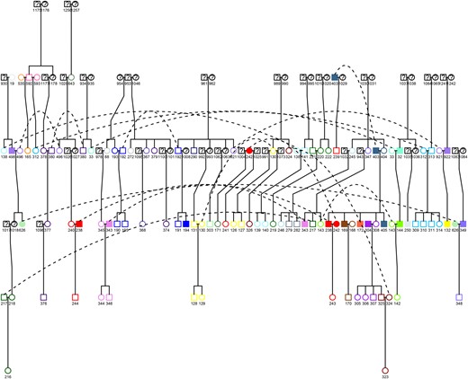
Pedigree tree of a subsample of the largest family. The pedigree tree was obtained using the Kinship2 R Package. Similar colors indicate the inhabitants living in the same house. Filled symbols denote infected individuals, empty symbols denote uninfected individuals, and question marks denote unknown status. Squares denote males, and circles denote females. Dotted lines indicate the same individual linking different regions of the pedigree.
Spatial Clustering Analysis
The study sample extended over 234 households for which GPS data were available (29 were missing georeferencing data, accounting for 62 individuals). For the total, adult, male, and female populations, the Moran index ranged from 0.008 to 0.037, and no values were statistically significant (P > .05). Similar results were found with the SPODT and SaTScan approaches (Table 2). Actually, only a marginally significant clustering was found in the population of children, with a Moran index of 0.132 (P < .001), a SPODT R2 at 0.309 (P = .040), and 1 cluster identified with SaTScan (P = .017). The position of this cluster (Figure 1) showed that very few children were concerned (5 cases for a total of 16 children in the significant SaTScan cluster). Therefore, the disease seems to be randomly distributed across the village.
Results of the Spatial Clustering Analysis
| Variable | Households or Residents, No.a | Moran Index | P (Moran) | R2 (SpODT) | P (SpODT) | SatScan | P (SatScan) |
|---|---|---|---|---|---|---|---|
| Total | 234 | 0.034 | NS | 0.043 | NS | 0 | NS |
| Adults | 234 | 0.037 | NS | 0.148 | NS | 0 | NS |
| Male | 195 | 0.009 | NS | 0.150 | NS | 0 | NS |
| Female | 211 | 0.008 | NS | 0.127 | NS | 0 | NS |
| Children | 147 | 0.132 | <.001 | 0.309 | .040 | 1 | .017 |
Abbreviation: NS, not significant.
a Global positioning system–available coordinates.
Familial Aggregation Analysis
The patterns of phenotypic correlations among different types of relative pairs, referred to as patterns of familial correlations, were examined for the 4 traits investigated (Table 3). Significant negative correlations were not observed for any of the traits. Both ICT positivity and ICT intensity did not show any significant correlation among relatives, whatever the degree of relationship. By contrast, for both MF positivity and MF density, we found strong significant correlations for many relative pairs. For both phenotypes, a significant positive correlation was found among parent-offspring pairs (ρparent–offspring = 0.45 and 0.44, respectively; both P < .05), while correlations between siblings were not significant. Interestingly, we noted a progressive decrease in the correlation coefficients with the genetic distance between relatives: correlation was highest among first-degree relatives (0.43 [P < .01]; and 0.37 [P < .05] for MF positivity and MF density, respectively), lower but still significant among second-degree relatives (0.12 [P < .05]; and 0.23 [P < .001], respectively), and not significant between more-distant relatives. Finally, when we focused on the subtypes pairs, we observed that, for both MF positivity and density, the statistically significant parent-offspring relationships ranged from 0.46 to 0.93. Interestingly, the correlations were significant when there was a male in the relationship, while correlations between mothers and daughters were not statistically significant.
Adjusted Intrafamilial Correlation Coefficients From the Familial Aggregation Analysis
| Variable | ICT Positivity | ICT Intensity | Microfilaremia Positivity | Microfilarial Density | ||
|---|---|---|---|---|---|---|
| Value | P Value | Value | P Value | |||
| 1st degree | 0.03 | −0.09 | 0.43 | <.01 | 0.37 | <.05 |
| Parent:offspring | −0.08 ± 0.36 | −0.23 ± 0.36 | 0.45 ± 0.15 | <.05 | 0.44 ± 0.17 | <.05 |
| Father:son | −0.09 ± 0.84 | −0.38 ± 0.69 | 0.46 ± 0.19 | <.05 | 0.68 ± 0.15 | <.01 |
| Father:daughter | −0.18 ± 0.41 | −0.30 ± 0.53 | 0.93 ± 0.09 | <.001 | 0.81 ± 0.25 | <.05 |
| Mother:son | 0.00 ± 0.47 | −0.09 ± 0.64 | 0.78 ± 0.23 | <.05 | 0.74 ± 0.22 | <.05 |
| Mother:daughter | −0.07 ± 0.89 | −0.07 ± 0.97 | 0.20 ± 0.40 | 0.19 ± 0.40 | ||
| Sibling | 0.18 ± 0.39 | 0.21 ± 0.46 | −0.18 ± 0.77 | 0.30 ± 0.17 | ||
| 2nd degree | −0.11 | −0.15 | 0.12 | <.05 | 0.23 | <.001 |
| Avuncular | −0.13 ± 0.19 | −0.16 ± 0.23 | 0.13 ± 0.03 | <.001 | 0.23 ± 0.03 | <.001 |
| Grandparent | −0.04 ± 0.38 | −0.15 ± 0.33 | 0.21 ± 0.17 | 0.29 ± 0.16 | ||
| 3rd degree | −0.04 | −0.03 | −0.16 | −0.17 | ||
| 4th degree | −0.12 | −0.04 | 0.30 | 0.20 | ||
Data are correlation coefficient ± standard error. The asymptotic standard error of a given correlation was estimated by using a second-order Taylor series expansion and replacing all correlation parameters with their respective estimates. Correlations were assessed for all available pair types. Results from saturated models and adjustments were individual risk factors (bed net, hunting, night in the bush, age, sex, and latrine) and environmental variables (road, main river, stream, dry creek, holes, and slate), with a household random effect.
Abbreviation: ICT, immunochromatographic test.
Heritability
Table 4 shows all adjusted heritability estimates derived from the variance components analysis. In the total population, heritability estimates were moderate for the infection status (0.23 [P = .06] for ICT positivity and 0.18 [P < .01] for ICT intensity) and very high and highly significant for the microfilaremia phenotypes (0.74 for MF positivity and 0.85 for MF density; both P < .001). A stratified analysis by age revealed similar results only in the adult population, with h2 estimates much lower and nonsignificant in children. Similarly, h2 values were lower and no more significant when they were estimated separately in males and females. Last, we found a significant household effect only for the ICT positivity and intensity traits and only in the female population (0.12 for both; P < .05).
Adjusted Heritability Estimates of Wuchereria bancrofti
| Variable | Total | Adults | Children | Male | Female | |||||
|---|---|---|---|---|---|---|---|---|---|---|
| h2 ± SE | c2 | h2 ± SE | c2 | h2 ± SE | c2 | h2 ± SE | c2 | h2 ± SE | c2 | |
| ICT ± | 0.23 ± 0.16 | 0 | 0.28 ± 0.24 | 0 | 0.08 ± 0.18 | 0.04 | 0.11 ± 0.30 | 0 | 0.13 ± 0.16 | 0.12a |
| ICT intensity | 0.18 ± 0.06b | 0 | 0.31 ± 0.14b | 0.01 | 0.13 ± 0.16 | 0.01 | 0.09 ± 0.15 | 0 | 0.04 ± 0.15 | 0.12a |
| MF ± | 0.74 ± 0.22c | 0 | 0.93 ± 0.27b | 0 | 0 | 0 | 0.24 ± 0.33 | 0 | 0.46 ± 0.36 | 0 |
| MF density | 0.85 ± 0.19c | 0 | 0.98 ± 0.10c | 0 | 0 | 0 | 0.62 ± 0.33a | 0 | 0.23 ± 0.40 | 0 |
Results from models using the following explanatory variables: individual risk factors (bed net, hunting, night in the bush, age, sex, latrine), environmental variables (road, main river, stream, dry creek, holes, and slate), with a household random effect.
Abbreviations: c2, variance component parameter accounting for shared environmental effects; h2, additive genetic component of variance (ratio of additive genetic variance to total phenotypic variance unexplained by covariates); ICT, immunochromatographic test; MF, microfilariae; SE, standard error.
aP < .05.
bP < .01.
cP < .001.
DISCUSSION
This study clearly evidenced a major role of genetics in the MF production trait considered both qualitatively (MF positivity) and quantitatively (MF density). Conversely, we did not find an important role of genetic factors in explaining the presence (ICT positivity) or the intensity (ICT score) of infection with W. bancrofti.
Despite our efforts to check all familial relationships composing the pedigrees, we cannot exclude that some links were false, especially some father-children links resulting from extraconjugal relations. The few studies conducted so far to assess paternity discrepancy showed that nonpaternity rates are generally low (between 1.7% and 3.7%) [23, 24]. In addition, as nonpaternity errors would dilute estimates of genetic linkage [25], we are confident in the robustness of our results: should a small proportion of false relationships be present in the pedigrees, the significance of the linkage would be underestimated.
Adjusted correlation coefficients for ICT traits were very low (none were statistically significant), indicating that familial susceptibility to infection is unlikely. However, a slight heritability for ICT intensity in the total population suggests that polygenic factors may be involved in the development of W. bancrofti infective larvae to adult worms and may thus explain the adult worm burden in an individual. However, this effect is likely to be marginal compared to the individual risk factors associated with exposure to mosquitoes. Thus, our results suggest that the acquisition of infection (ie, the presence of adult worms) in Séké Pembé is likely to be mainly driven by environmental factors and individual habits. This could mean either that the coevolution between host and parasite is relatively recent, or, more likely, that the cost to the host would be too deleterious to establish a defense system dedicated to adult worm acquisition. Age-, sex-, and activity-dependent exposure to mosquitoes were shown to be important risk factors for infection with W. bancrofti in our study population, which is consistent with previous epidemiological findings [16]. However, our results contrast with the study conducted in a Pacific island, where genetic factors were shown to play a major role in the acquisition of infection, with a heritability estimate of 0.46 [13]. Actually, heritability corresponds to the phenotype variability explained by genetic factors and is specific to a population in a given environment [14], and it could be interpreted as a balance between the environmental pressure and the role of genetic factors. Therefore, we could either imagine that the population in the island studied may have less genetic diversity than the Séké Pembé population, that environmental factors were not taken enough into account in the former study, or that environmental factors did not really discriminate between the inhabitants. Indeed, in contrast to Cuenco et al, we included age, sex, but also previously identified individual risk factors and several environmental variables in our models.
Interestingly, heritability was higher in the adult population than in children for both ICT positivity and ICT score and was significant in the adults for ICT score. This may reflect the fact that children did not have time to develop their infection. This may also reflect a differential implication of genetics according to age, and consequently, could be indicative of the involvement of adaptive immunity rather than innate immunity. This result may support the existence of herd immunity [26], this regulation depending on the burden of adult worms. Furthermore, it is noteworthy that h2 estimates were similar between males and females for both ICT traits, suggesting that the classical but not universal sex difference mainly depends on habits-related exposure differences rather than genetic factors.
Conversely, MF traits were found to be strongly influenced by genetic factors in our population, with high and significant correlation coefficients among close relatives (first-degree and, at a lesser extent, second-degree relatives). Genetic factors explained >70% of the phenotypic variance for the MF producers. This is consistent with the results obtained by Cuenco et al [13] and with the statement that a maximum of 50% of ICT-positive individuals are microfilaremic around the world [27]. Moreover, our familial aggregation analysis strengthened this last statement, since we found an intrafamilial correlation coefficient of 0.43 for the parents of first degree. This result also highlights a recent study showing that the transforming growth factor β1 Leu10Pro variant is involved in the status regarding microfilaremia (positivity and density) [11]. Interestingly, we observed that the correlations were only significant when a male was involved in the relationship, the mother-daughter correlation being low and not significant. Since we adjusted on individual habits (ie, hunting especially in males), this result should show a real genetic effect. We have no explanation for this result, which deserves further investigations.
Similarly to ICT traits, a differential heritability between adults and children was observed for MF status, with a major role of genetic factors being evidenced only in the adults. This suggests that an adaptive immunity response is likely to be involved in the regulation of MF production. An elevated adapted immune response is known to be associated with latent infections and has been shown to especially involve interleukin 5 [4]. This is particularly interesting in view of the recent finding that interleukin 5 levels mainly depend on heritable influence [28]. Finally, we observed that heritability regarding MF density was much higher in males than in females and significant only in this subpopulation (0.62; P < .05). This result, together with the findings of the familial aggregation study, strengthen the idea that the genetic factors involved in the MF production could be related to specific male factors.
In conclusion, the acquisition of W. bancrofti infection seems to be mainly influenced by environmental factors, although an adaptive immunity may exist in adults, especially for the regulation of the number of adult worms. By contrast, the MF production is strongly mediated by additive genetic factors. A study aiming to better understand the possible specific male factors underlying the high heritability observed in this sex could be interesting.
Notes
Acknowledgments. We thank the residents of Séké Pembé, for their active participation; the secretaries (especially Paul Bakala); the chiefs (Bernard Mvoula and Maurice Boukouma), for their help with the pedigree construction; and the staff of the Ministry of Health and Population of the Republic of Congo who participated in the study.
Disclaimer. The funders had no role in study design, data collection and analysis, decision to publish, or preparation of the manuscript. The findings and conclusions contained within are those of the authors and do not necessarily reflect positions or policies of the Bill and Melinda Gates Foundation.
Financial support. This work was supported by the Bill and Melinda Gates Foundation, as part of the Death to Onchocerciasis and Lymphatic Filariasis project (Dr Gary J. Weil, principal investigator).
Potential conflicts of interest. All authors: No reported conflicts. All authors have submitted the ICMJE Form for Disclosure of Potential Conflicts of Interest. Conflicts that the editors consider relevant to the content of the manuscript have been disclosed.
References
Author notes
Presented in part: 64th Annual Meeting of the American Society of Tropical Medicine and Hygiene, Philadelphia, Pennsylvania, 25–29 October 2015. Poster 459.

