


Abstract
Over the last 70 years, many advanced countries have experienced growing real house prices and an increasing housing wealth-to-income ratio. To explain these long-run patterns, this paper introduces a novel multi-sector growth model where housing services are produced using non-reproducible land and reproducible structures. Land is also employed in the non-housing sector. First, we identify two fundamental mechanisms driving the long-run increase in the real house price: (i) technological progress in the construction sector lags behind the technological progress of the rest of the economy and (ii) housing production is more land-intensive than non-housing production. Second, we study transitional dynamics for the US, UK, France, and Germany. Our calibrated model explains most of the observed increase in the housing wealth-to-income ratio since 1950. Counterfactual experiments identify initially low stocks of residential structures and non-residential capital as key exogenous drivers for this increase. The associated investment incentives led to a long-lasting construction boom and steadily increasing land scarcity, boosting residential land prices.
1. Introduction
Housing wealth is the largest private wealth component. Figure 1 displays its size, scaled by aggregate income, over time for the US, UK, France, and Germany since 1950. Housing wealth has grown considerably faster than income. In 1950, the aggregate housing stock was on average worth 1 year of aggregate income; by the end of our sample period, this value had risen to almost 4 years of aggregate income. Housing wealth also grew faster than non-housing wealth, serving as a primary factor in the overall wealth increase. The decomposition of housing wealth into residential land and residential structure wealth reveals that residential land wealth has increased enormously in all four economies, being responsible for most of the increase in housing wealth.
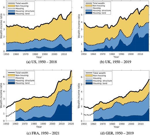
Wealth-to-income ratio: the relevance of housing. The housing wealth-to-income ratio is the sum of the aggregate value of residential structures and the aggregate value of residential land, both relative to income. Data on residential structure wealth and land wealth in Germany and France start in 1960, as indicated by the white space before 1960 in Figures 1c and 1d. The data sources are described in Online Appendix A.
Housing wealth is the product of house price and house quantity. Knoll, Schularick, and Steger (2017) examine the evolution of real house prices in 14 advanced economies since 1950 and find that, on average, they have tripled. The non-reproducible factor land, once again, seems to be the main driver behind this upward trend. While the real price of structure increased annually by an average of 0.9% in the US, UK, France, and Germany since 1950, the real price of residential land grew by almost 5% annually.1
Why have house prices and the housing wealth-to-income ratio been increasing in the US, UK, France, and Germany since 1950? In this paper, we provide a novel long-run theory to answer this question. We employ a Ramsey growth model with two main sectors, a numeraire sector and a housing sector. The numeraire sector employs labor, physical capital, and non-residential land to produce a consumption–investment good. The novel part of our model is the supply side of the housing sector. This sector comprises three types of firms. Land development firms purchase land and transform it into residential land by utilizing labor. Construction firms manufacture structures by employing materials and labor. Property management firms combine residential land and residential structures to produce houses they rent out to households. The latter follows the empirical work by Davis and Heathcote (2007), who “[...] conceptualize a house as a bundle comprising a reproducible tangible structure and a non-reproducible plot of land”. This decomposition is further substantiated by a set of stylized facts we provide. Accordingly, the real price of residential land has been growing at a considerably higher rate than the real price of residential structures, while the quantity of residential land has been growing by less than that of residential structures in the US, UK, France, and Germany since 1950. To understand this mirror-like pattern, it is essential that reproducible structure and non-reproducible land are modeled as two distinct endogenous stocks and that the overall land supply is fixed in the long run. Another feature of the model that turns out to be crucial is differential technological progress. We allow technological growth to differ between the numeraire and residential construction sectors.
Why is the increase in the house price and the housing wealth-to-income ratio relevant for the macroeconomy? First, rising house prices and rents have raised concerns about the affordability of housing (Quigley and Raphael 2004; Albouy, Ehrlich, and Liu 2016). Because the representative household must devote a higher multiple of income to purchase the existing housing stock, the increase in the aggregate housing wealth-to-income ratio points to a potential affordability issue. Second, Gennaioli, Shleifer, and Vishny (2014) argue that the long-run increase in the share of financial sector income in GDP is driven by a rising total wealth-to-income ratio. Figure 1 shows that this increase is mainly driven by housing wealth. Similarly, based on historical data for 17 advanced economies, Jordà, Schularick, and Taylor (2016) document a pronounced increase in the credit-to-GDP ratio in the 20th century. Namely, they argue that rising mortgages and housing wealth are mainly responsible for this increase.2 Lastly, the long-run increase in the total wealth-to-income ratio contributes to a change in the functional income distribution to the advantage of capital income recipients (Piketty and Zucman 2014). These distributional implications resonate with the view presented in Karl Marx’s “Das Kapital” (Marx 1867), elucidating the analogy in our title. The housing sector seems especially important in this context, as stressed by Rognlie (2015). He argues that the increase in the aggregate capital income share in the G7 economies over 1950–2010 is driven exclusively by the housing sector. Because the yield component of the rate of return on housing has been reasonably stable (Jordà et al. 2019), the increase in the housing component of the capital income share has to be driven by an increase in the housing wealth-to-income ratio.3 Understanding, why the house price and housing wealth-to-income ratio have been increasing, is crucial for these three debates.
We proceed in two steps to explain why, based on our theory, the house price and the housing wealth-to-income ratio increased since the 1950s. First, the tractability of the model allows us to obtain closed-form steady-state solutions. Thus, we show under what conditions the house price grows in the long run. Second, a rising wealth-to-income ratio cannot be explained in a steady state.4 Thus, we bring our model to the data by studying transitional dynamics for the US, UK, France, and Germany.
Two mechanisms explain an increasing real house price in a steady state. First, the more land-intensive the housing sector is compared with the numeraire sector, the higher the long-run growth rate of the house price. Thus, the crucial aspect is not merely the fixed nature of the production factor land. It is rather the relative intensity with which land is used in both sectors. Second, if technological growth in the numeraire sector outpaces that in the construction sector, the house price will grow at a higher rate in the long run. Empirical evidence and our model calibration validate both mechanisms. Our calibration attributes one-third of the steady state growth rate in the house price to differences in land intensities and two-thirds to differential technological growth.
To study the evolution of the housing wealth-to-income ratio since 1950, we calculate transitions for the US, UK, France, and Germany. We calibrate the model by matching a set of moments along the transition separately for each of the four economies. In doing so, we abstain from matching the increase in the housing wealth-income ratio or the house price and let the model speak to the evolution of these variables. We also feed in exogenous series for population, the employment-to-population ratio, and construction sector productivity. For the UK, France, and Germany, the calibrated model explains 84%, 70%, and 63% of the increase in the housing wealth-to-income ratio since 1950, respectively. In the US, the model’s prediction exceeds the actual increase in the housing wealth-to-income ratio since 1950 by 20 percentage points. We show that the calibrated model is also consistent with the observed post-war construction boom in the US, that is, a fast accumulation of structures,5 the observed near-constancy of structure prices over time, and the observed surge in land prices.
To understand what exogenous drivers—through the lens of our model—are responsible for the observed increase in house prices and the housing wealth-to-income ratio, we conduct counterfactual experiments. We first asses the role played by the exogenous dynamics in population size, the employment-to-population ratio, and construction productivity growth by holding all of them constant at their 1950 level. The observed rise in the house price can, to some degree, be attributed to rising population size because it raises housing demand and thus prices of land and houses. However, the dynamics of all three exogenous state variables explain little of the increase in the housing wealth-to-income ratio. Our analysis suggests that neoclassical convergence forces explain the evolution of the housing wealth-to-income ratio: initial values of physical capital and residential structures—exogenous model variables in the initial period—were considerably below their steady-state values in all considered economies. Intuitively, a low stock of residential structures implies a high marginal productivity of structures in producing housing services, leading to high residential investment at the start of the transition. An initially low and subsequently growing capital stock results in rising housing demand and a declining interest rate, pushing the house price up. We interpret low levels of capital and residential structures in 1950 as a result of underinvestment pre-1950 due to low savings after the Great Depression, redirection of investment to support the war, and destruction of capital and residential structure in the case of Continental Europe.
The rest of the paper is organized as follows. In Section 2, we discuss our contribution to the related literature before presenting five stylized facts on the housing wealth-to-income ratio and its decomposition into quantities and prices in Section 3. Section 4 sets up the model and defines an equilibrium. The main sections are Section 5, where we present our steady-state results on house price growth, and Section 6, where we explain the growth in the housing wealth-to-income ratio since 1950. In Section 7, we discuss additional channels and observations before concluding in Section 8.
2. Related Literature
In exploring the long-run rise in housing wealth and house prices, this paper contributes to the growing literature on housing and macroeconomics. We organize the subsequent discussion into three blocks: empirical literature, theoretical literature focused on short-run phenomena, and theoretical literature dedicated to long-run phenomena.
The first branch of this literature is primarily concerned with the measurement of aggregate housing wealth and house prices. Davis and Heathcote (2007) are among the first to estimate residential land wealth and prices for the US. Piketty and Zucman (2014) document the evolution of the aggregate wealth-to-income ratio for eight developed economies from 1700 to 2010, showing that it has risen since the 1970s. Relatedly, Rognlie (2015) argues that the housing sector has driven the surge in the net capital income share since 1948. Turning to house prices, Knoll, Schularick, and Steger (2017) provide annual house prices for 14 advanced economies since 1870. They show that real house prices started to rise in the second half of the twentieth century, driven mainly by a pronounced increase in land prices, not construction costs.
We base our stylized facts on the existing empirical literature, emphasizing that most of the increase in housing wealth comes from the rise in residential land wealth. Our primary contribution, however, is in offering a theory to explain the documented growth in house prices and housing wealth.
Second, since the US housing bust and the subsequent Great Recession, many studies contributed to a better understanding of the relationship between housing and the macroeconomy over the short run. One of the earlier papers in this field is by Davis and Heathcote (2005), who set up a neoclassical multisector stochastic growth model to investigate the cyclical dynamics of residential investment and other business cycle facts. The housing supply side of their model forms the basis for many subsequent models. For instance, Favilukis, Ludvigson, and Nieuwerburgh (2017), employing a quantitative heterogeneous agent model, find that the relaxation of financing constraints and its subsequent reversal was the driving force behind the recent US-housing boom and bust. Kaplan, Mitman, and Violante (2020) come to a different conclusion. Accordingly, it is not the relaxation of financing constraints that drives house prices in the short run but rather changes in beliefs about the likelihood of future housing demand shifts. Whether credit conditions were responsible for the boom and bust in house prices is an ongoing debate. Greenwald and Guren (2019) provide a reconciliation by showing that the segmentation of housing markets matters for the transmission of credit supply shocks.
We do not study short-run fluctuations in housing wealth but focus on the long run. Moreover, the housing supply side of our model differs from these existing models for two reasons. First, existing macro models with housing assume that each period one unit of land becomes available and is incorporated into the housing stock by the construction sector. When explaining the evolution of housing wealth, we decompose it into price and quantity components of residential land and structures. Assuming that the quantity of residential land is exogenous would restrict the analysis of the long-run evolution of residential land with strong implications for the residential land price. Second, existing models assume that land is not productive in the numeraire sector. This assumption places a strong restriction on differential land intensities of the numeraire and the housing sector. Our analysis shows that differential land intensities play an important role in the determination of long-run rent and house price growth.
Lastly, we share our focus on housing over the long run with a smaller branch of the literature on housing and macroeconomics. Hansen and Prescott (2002) employ a one-good, two-sector overlapping generations (OLG) model where land is in fixed supply.6 They argue that the transition from constant to growing living standards is inevitable given positive rates of total factor productivity growth. In particular, the transition from stagnant to growing living standards occurs when profit-maximizing firms, in response to technological progress, begin employing a less land-intensive production process that, although available throughout history, was not previously profitable to operate. Martin (2005) presents a dynamic two-sector general equilibrium model based on the Lucas asset price framework but without capital accumulation and production. He investigates demographic shifts, demonstrating that the US baby boom can account for certain trends in US house prices and interest rates since the 1960s. Herkenhoff, Ohanian, and Prescott (2018) construct a general equilibrium spatial growth model of the US to analyze how state-level land-use restrictions have impacted regional and aggregate economic activity between 1950 and 2014. Tightened land use restrictions, they argue, have increasingly limited the availability of land for housing and commercial use, which have raised land prices, slowed interstate migration, reduced factor reallocation, and depressed output and productivity growth relative to historical trends. Borri and Reichlin (2018) employ a two-sector OLG model with housing services and bequests to show that a rising labor efficiency in the general economy relative to the construction sector pushes the house price, the housing wealth-to-income ratio, and wealth inequality upwards. Due to inelastic housing demand, an increase in relative labor efficiency triggers not only a strong house price appreciation but also a reallocation of resources to the housing sector. Miles and Sefton (2021) employ a spatial Ramsey growth model with two sectors. Residential land is endogenous and depends on the state of transport technology. They derive a condition under which the speed at which transport technology improves relative to the growth in aggregate incomes is such as to generate flat house prices in a growing economy. The model can explain the constancy of the real house price before 1950 and the surge thereafter.
While we share the focus on housing over the long run with this literature, our model differs as it explicitly differentiates between (i) the stock of residential land and residential structures, (ii) differential technological progress, and (iii) differences in land intensities between the housing and non-housing sectors. The latter allows us to assess the relevance of each of the two mechanisms in driving house prices in the long run. Furthermore, our main focus lies in explaining not only the house price evolution but also the rising housing wealth-to-income ratio.
3. Stylized Facts
This section provides a list of stylized facts related to housing and macroeconomics. While the data underlying these facts is not new, the compilation of five housing-related macroeconomic facts presents a novel perspective. The data sources are described in Online Appendix A. This set of empirical data is instrumental in better understanding the long-run evolution of house prices and housing wealth. Additionally, it serves to discipline a theory aiming to explain these variables.
Before discussing the data, we introduce a minimal set of concepts essential for understanding the first three facts. Following Davis and Heathcote (2007), we decompose housing wealth into the sum of the value of structures and the value of residential land,
Moreover, each wealth component can be decomposed into a price and a quantity component according to
where |$P^{\text{housing}}$| denotes a house price index, |$Q^{\text{housing}}$| is a quantity index for the housing stock, and the notation for structure and land is similar.
We study data for France, Germany, the UK, and the US from various sources for the period 1950 up until 2021. For some variables and countries, observations are only available from 1960 or only until 2012. Table 1 puts numbers on each stylized fact. We elaborate on each of the five stylized facts in the following.
Average growth in housing-related variables since 1950.
| Fact | Average annual growth of | US | UK | FR | DE |
|---|---|---|---|---|---|
| 1 | wealth-to-income ratio (in %) | 0.9 | 0.7 | 1.9 | 1.6 |
| housing wealth-to-income ratio (in %) | 0.7 | 1.8 | 2.8 | 2.2 | |
| non-housing wealth-to-income ratio (in %) | 0.5 | -0.2 | 0.7 | 0.7 | |
| 2 | house price (in %) | 1.1 | 2.3 | 4.5 | 1.4 |
| residential land price (in %) | 3.5 | 3.7 | 9.7 | 1.7 | |
| residential structure price (in %) | 0.3 | 1.2 | 0.7 | 1.2 | |
| 3 | house quantity (in %) | 2.3 | 1.9 | 1.2 | 2.9 |
| residential land quantity (in %) | 1.6 | 1.3 | 1.2 | 2.5 | |
| residential structure quantity (in %) | 2.7 | 2.5 | 3.7 | 3.1 | |
| 4 | housing rent (in %) | 0.9 | 1.6 | 3.1 | 0.8 |
| 5 | land share in housing wealth (in pp) | 0.3 | 0.4 | 0.7 | 0.6 |
The values are average annual growth rates in percent, except for the land share, where the values are average annual differences in percentage points. The period starts in 1950 and ends around 2020 with the following exceptions: House price data for Germany, including residential land and residential structure prices, from 1962 onwards. Residential land prices ended in 2012 for the UK, France, and Germany. Data on residential structure wealth and land wealth for Germany and France start in 1960. The data sources and covered periods are described in Online Appendix A.
(Wealth). The wealth-to-income ratio has increased, as depicted in Figure 1, a trend highlighted by Piketty and Zucman (2014). When breaking down this ratio into housing and non-housing components, it is evident that the housing wealth-to-income ratio has surged more prominently than its non-housing counterpart, as also illustrated in Figure 1.7 This observation is consistent across all four economies, with the disparity being notably marked in the UK and France, as detailed in Table 1.
(Prices). Real house prices, real construction costs, and real land prices have increased in all four countries. The increases have already been documented for the US by Davis and Heathcote (2007) and for a group of 14 advanced economies by Knoll, Schularick, and Steger (2017).8 According to Table 1, real house prices have roughly doubled since 1950 in the US, as implied by an average growth rate of 1.1% over almost 70 years. Average growth rates are even higher in the UK, Germany, and France, with 2.3%, 1.4%, and 4.5%, respectively. Comparing residential structure price changes with residential land price changes reveals a striking pattern. Residential land prices exhibited strong growth, while the prices of residential structures rose only modestly. Given Figure 1, showing that structure wealth remained relatively stable relative to income, this suggests that the increase in residential land prices is responsible for much of the increase in the housing wealth-to-income ratio.
(Quantities). We compute quantity indices by using the value indices and price indices for overall housing, residential land, and residential structures. The quantity index of residential structures has been steadily increasing, while the quantity index of residential land increased modestly. Taken together, facts 2 and 3 point to a mirror-like pattern. While the quantity of structure increased strongly, its price increased only moderately. For residential land, the reverse holds; the price increased much stronger than the quantity. This observation points to an essential role of the economy’s supply side. Residential structure is reproducible, implying a higher price elasticity of supply, while residential land is nonreproducible in the long run, implying a lower price elasticity of supply. This observed mirror-like pattern guides our modeling choice, and we will return to it frequently.
(Rents). The housing rent—the price of the service flow derived from the stock of housing—has grown at a positive rate but more slowly than the house price—the price of the stock of housing. The average annual growth rate ranges between 0.8% in Germany and 3.1% in France, as shown in Table 1. Fact 4 has been stressed by Knoll (2017) and Jordà et al. (2019).
(Land). Finally, it is helpful to decompose the housing wealth-to-income ratio into a residential structure and residential land component as defined in equation (1) to understand why it has been increasing. A variable that compactly summarizes the contribution of these two factors is the share of land wealth in total housing wealth.9 As can be inferred from Figure 1 and seen in Table 1, this share increased considerably, averaging 0.3–0.7 percentage points per year. A plausible theory replicating the increase in the housing wealth-to-income ratio—Fact 1—shall also align with facts 2–5. We will come back to all the facts below.
4. The Model
Consider a perfectly competitive closed economy. Time is continuous and indexed by |$t \in \mathbb {R}$|. Infinitely-lived households earn labor and capital income, save, and consume two goods: housing services and a non-housing good. The two consumption goods are produced by two different sectors, a numeraire sector and a housing sector.10 The numeraire sector combines physical capital, labor, and land to produce an output good. The output of this sector can be consumed, invested into physical capital, or used as an input in the construction sector. The innovative part of our model concerns the housing sector. This sector comprises three types of firms. First, property management firms purchase residential land and residential structures to produce houses, generating revenues from renting to households. Second, construction firms manufacture structures by employing materials and labor. Third, land development firms develop residential land by purchasing non-developed land and employing labor. The overall land supply is fixed, and the intersectoral land allocation is endogenous. In steady-state equilibrium, economic growth is driven by exogenous technological change.
4.1. Households
The economy is inhabited by mass one of households. A household consists of |$S_t \gt 0$| homogeneous members. Total population is hence equal to |$S_t$|. We allow |$S_t$| to grow over time. Households consume two goods, housing services, |$D_t$|, and a non-housing good, |$C_t$|. We denote all prices in units of the latter. The representative household derives utility from consumption streams |$\left\lbrace C_t, D_t \right\rbrace _{t=0}^\infty$| according to
where |$\rho \gt 0$| is the time preference rate and |$u\left( C_t/S_t, D_t/S_t \right)$| the period utility function with per-capita consumption of the numeraire and per-capita housing services as arguments. Household utility at t is the product of household size, |$S_t$|, and per-capita utility, |$u\left( C_t/S_t, D_t/S_t \right)$|. The period utility function has the following form11:
such that |$\sigma \gt 0$| is the inverse of the intertemporal elasticity of substitution (IES) and |$\theta \in (0,1)$| the housing expenditure share.
We allow total population and total labor supply to differ because—as will be shown further below—the two evolve differently in the data, exerting different effects on the house price.12 Each household supplies |$N_t$| units of time inelastically to the labor market. Aggregate labor supply then equals |$N_t$|, while per-capita labor supply equals |$N_t / S_t$|. A household’s total wealth is given by W, generating a flow return of |$r W$|. The budget constraint reads
where q is the price of housing services, w is the wage, and |$\Pi ^L$| are profits of firms that develop land, as specified below.13 Saving, |$\dot{W}$|, and total consumption expenditures equal total income, including wealth income, earnings, and profits.
4.2. Numeraire Production
Mass one of firms produce the numeraire good, Y, with inputs capital, K, labor, |$N^Y$|, and land, |$L^Y$|, according to
where |$\alpha ,\beta \in (0,1)$| and |$\alpha +\beta \lt 1$|. Changes in variable |$B^Y$| capture exogenous labor-augmenting technological progress. In the long run, |$B^Y$| grows at the constant rate |$g^Y \in \mathbb {R}$|. Throughout the paper, we will primarily employ Cobb–Douglas production functions. If we used more general CES functions with an elasticity of substitution (EoS) unequal to unity, a steady state with differential technological growth would not exist.
The representative firm solves the following problem:
where |$\delta ^K \ge 0$| is the capital depreciation rate and |$R^{LY}$| the rental rate of non-residential land.
4.3. Housing Sector
A house is a bundle of two conceptually different stocks: underlying land, |$L^H$|, and the residential structure, X, erected upon it. This distinction follows the empirical contribution by Davis and Heathcote (2007), who provide price and quantity indices for housing, land, and structures for the US and show that this distinction is key for understanding aggregate housing market dynamics. This distinction is also necessary for mapping model outcomes to the stylized facts presented in Section 3. The main difference between |$L^H$| and X is that the former is not reproducible in the long run, while the latter is. Increasing housing demand over time implies that X can be accumulated, while |$L^H$| cannot. Consequently, prices for X will increase less than prices for |$L^H$|.
The housing sector consists of three different subsectors.14 First, property management firms demand residential structures and residential land to build houses rented out to households. Second, construction firms demand labor and materials to produce new structures that are sold to property management firms. Lastly, land development firms demand labor and non-developed land to produce residential land and sell it to property management firms. We now go through each of these activities in turn.
4.3.1. Property Management
Property management firms combine residential structures, X, and residential land, |$L^H$|, to produce houses, H, according to
where |$\gamma \in [0,1)$|. The stock of houses H generates a proportional flow of housing services equal to H.15 Housing services are sold to households at the rental rate q. Property management firms manage the existing housing stock and invest in additional houses. They commission construction firms to produce |$I^X$| new units of structure at a price |$P^X$| and land developers to produce |$I^L$| new units of residential land at the price |$P^{LH}$|. The representative property management firm solves the following dynamic problem:
where
are the firms’ cash flow and cumulative discount rate. The cash flow consists of revenues from renting out the existing housing stock, |$q H$|, minus investment expenditures. The laws of motion of structures and land reflect that structures depreciate at the rate |$\delta ^X \in [0,1],$| while land does not. This difference in depreciation is a plausible assumption because maintaining a constant housing stock necessitates replacement investment into structures. However, it is unnecessary to produce additional land to keep the housing stock constant.
The property management firm’s assets can (i) either be expressed as the value of residential structures plus the value of residential land, |$P^{LH} L^H + P^X X$|, or (ii) as the value of houses, |$P^H H$|, where |$P^H$| is the house price. This equivalence reflects that houses are bundles of structure and land. Since the two have to be equal, |$P^{LH} L^H + P^X X = P^H H$|, the resulting house price reads
The house price is a weighted sum of the prices of residential land and residential structures. The weights are the land and structure intensity in housing, respectively.
Households own the property management firms. The aggregate valuation of property management firms is given by the value of its assets, |$P^H H$|. Without loss of generality, we set the number of shares equal to H such that the share price equals |$P^H$|. This normalization implies that the price of a house and the value of a share is equal to |$P^H$|, and households effectively trade houses, which they ultimately own. Owning one share entitles the owner to a yield of |$R^H = q - \delta ^X P^X X / H$|. The yield is rental income minus depreciation per unit of housing.
4.3.2. Construction
The representative construction firm employs materials, M, and labor, |$N^X$|, to produce new structures according to
where |$\eta \in [0,1)$|. A change in variable |$B^X$| captures the exogenous technological change in the construction sector. In the long run, |$B^X$| grows at the constant rate of |$g^X \in \mathbb {R}$|. The representative firm chooses labor and materials to maximize profits according to
where |$P^X$| is the price of residential structures. Materials are intermediate goods produced with the same technology with which the numeraire good is produced. Therefore, their price is equal to 1.
4.3.3. Land Development
The economy’s land endowment is denoted by L. It is allocated between the housing and numeraire sectors such that |$L = L^H_t + L^Y_t$| holds in equilibrium. In order to make land suitable for housing, it has to be developed by land development firms. These firms purchase (or sell) |$\dot{L}^Y$| units of non-developed land in order to increase (or decrease) the stock of developed land by |$\dot{L}^H$| units. We use the terms residential land and developed land interchangeably. Total land L is constant such that the total amount of land that can be used economically is fixed. For a long-run exploration of the macroeconomics of housing, this seems more plausible than the opposite—ever-growing land supply.16 Reallocating land from one sector to the other is costly. The representative land development firm chooses investment into residential land |$I^L \gtreqless 0$| to maximize profits according to
where |$P^{LH}$| and |$P^{LY}$| are prices of developed land and non-developed land, respectively, and |$N^L = \mathcal {N}^L (I^L)$| is the labor input associated with the reallocation of land. We assume that this cost function takes the form
where |$\xi \ge 0$| captures the importance of adjustment cost. These cost arise from activities like pulling down an existing building, leveling the surface off, and installing utilities like sewage, water, electricity, or roads.
If |$\xi =0$|, the reallocation of land is costless. The land allocation would be a jump variable as |$L^H$| and |$L^Y$| adjust immediately until |$P^{LH} = P^{LY}$| is restored at each instant.17 Although the model allows for this immediate rededication of land, we show in the calibration section that this is empirically implausible.
If |$\xi \gt 0$|, the reallocation of land is costly, and firms will choose an interior optimum. In this case, land reallocation is stretched over time, and |$L^Y$| and |$L^H$| are state variables. The first-order condition (FOC) for equation (16) reads
In equilibrium, the adjustment cost are |$w N^{L} = \left( P^{LH} - P^{LY} \right)^2 / \left(2 \xi w \right)$|, and profits can be expressed as |$\Pi ^{L} = w N^{L}$|. The price difference between residential and non-residential land, |$P^{LH}-P^{LY}$|, determines whether firms develop residential land and how much they develop. First, if residential land is more valuable than non-residential land, firms engage in land development and |$I^{L}$| > 0. Profits, which are strictly positive, are distributed to households who own land development firms. Second, firms do not reallocate land if land prices are equal and profits and adjustment cost are zero. Lastly, land development firms not only develop residential land but also conduct reverse activity when the price of non-residential land is higher than the residential land price. In this case, |$I^{L}$| is negative, and land is reallocated from the housing to the numeraire sector. Profits and adjustment cost are also positive in this case.18
The land development sector becomes inactive in the long run. Since total land endowment is fixed, there will be no land reallocation, and therefore land prices will equalize such that |$N^{L} = I^{L} = \Pi ^{L} = 0$|. Hence, the land development sector matters only for transitional dynamics.
4.4. Assets
The assets in this economy are (i) capital, K, (ii) non-residential land, |$L^Y$|, and (iii) houses, H. All assets are ultimately owned by households, as can be seen in the decomposition of total household wealth
Total wealth consists of housing wealth and non-housing wealth, where the latter is the sum of capital and non-residential land. Because markets are complete and the economy is deterministic, all assets yield the same rate of return, r, in equilibrium19
The return to housing H consists of capital gains, |$ \dot{P}^X X / H + \dot{P}^{LH} L^H / H$|, and rental income, |$R^H$|. Capital gains are the weighted sum of the underlying structure and land price changes.
Households are indifferent about the allocation of total wealth, W, across the different assets and care only about total wealth W and the rate of return r. It is, therefore, sufficient to consider only total wealth, W, and r instead of all assets in the household problem.
4.5. Equilibrium
We define the competitive equilibrium next.
(Competitive equilibrium). A competitive equilibrium of the model are sequences |$\big \lbrace C_t$|, |$D_t$|, |$W_t$|, |$q_t$|, |$w_t$|, |$r_t$|, |$\Pi ^{L}_t$|, |$Y_t$|, |$K_t$|, |$N^Y_t$|, |$L^Y_t$|, |$R^{LY}_t$|, |$H_t$|, |$R^H_t$|, |$X_t$|, |$L^H_t$|, |$P^X_t$|, |$CF_t$|, |$I^{L}_t$|, |$N^{L}_t$|, |$P^{LH}_t$|, |$P^{LY}_t$|, |$P^H_t$|, |$I^X_t$|, |$M_t$|, |$N^X_t \big \rbrace _{t=0}^\infty$| for given initial capital, residential land, and residential structures |$\lbrace K_0, L^H_0, X_0\rbrace$| and exogenous population, labor supply, and technology sequences |$\left\lbrace S_t, N_t, B^Y_t, B^X_t \right\rbrace _{t=0}^\infty$| such that
households maximize equation (3) given equation (4) subject to equation (5) and a no-Ponzi game condition;
firms in the construction sector and the numeraire sector, land developers, and property management firms maximize profits as given by equations (7), (9), (15) and (16), taking equation (17) and prices as given;
rental market clears: |$H_t = D_t$|;
labor market clears: |$N^X_t + N^Y_t+ N^{L}_t = N_t$|;
land market clears: |$ L^H_t + L^Y_t = L$|;
asset markets clear equation (19);
the house price is given by equation (13);
there are no arbitrage opportunities between assets, as described by eqaution (20).
The market for the numeraire good clears by Walras’ law.
4.6. Housing Wealth-to-Income Ratio
In order to express the housing wealth-to-income ratio, we need first to define the economy’s income consistently with the empirical convention of using the net national product (Piketty and Zucman 2014; Rognlie 2015). It is denoted by net national income |$(NNP)$| and given by
Since the economy comprises four production sectors, GDP equals the sum of the value-added of these sectors. In order to avoid double accounting, materials M have to be subtracted from construction output because they are intermediate goods. Value added from the land development sector is always positive because |$I^{L}$| has the same sign as the land price difference |$P^{LH}-P^{LY}$| such that |$I^{L} \times \left( P^{LH}-P^{LY} \right) \ge 0$|. Rededicating land from the numeraire sector to the housing sector enables land developers to create value added. This value added equals the value of newly developed land, |$P^{LH} I^{L}$|, reduced by the costs for the purchase of non-developed land, |$P^{LY} I^{L}$|. Subtracting depreciation from GDP yields net domestic product. Net domestic product is equal to NNP because the model economy is closed. Using equation (13), the housing wealth-to-income ratio is—in line with the empirical measurement of Section 3—given by
The total wealth-to-income ratio and the non-housing wealth-to-income ratio are defined similarly. Equation (23) shows that the housing wealth-to-income ratio can be decomposed into the residential land wealth-to-income ratio and the residential structure wealth-to-income ratio. The model directly maps total wealth, prices, and quantities of houses, residential land, and residential structures into the data.
4.7. Relation to Existing Theories
How does the model differ from existing macroeconomic models with a housing sector? First, the model distinguishes two endogenous stocks, namely, residential land and residential structures. Both stocks are essential input factors in the production of housing services and both stocks represent the two components of housing wealth. Existing macro models with housing assume that each period one unit of land becomes available and is incorporated into the housing stock by the construction sector.20 We depart from this model structure because it would be ill-suited to investigate the evolution of housing wealth and its components over the long run. Recall that we decompose housing wealth into four components: the price and quantity components of residential land and the price and quantity components of structures. Assuming that the quantity of residential land is exogenous would restrict the analysis of the long-run evolution of residential land with strong implications for the residential land price.
Second, most existing macro models with housing assume that the numeraire sector does not employ land. In the context of our research question, this would be a further restrictive assumption. Below we show that long-run growth in rents and house prices is driven by differential technological change and differential long-run land intensities. Assuming land is not productive in the numeraire sector implies a strong and restrictive assumption with regard to relative long-run land intensities. This assumption would impose an important constraint on the numerical analysis.
Third, the existing macro model with housing would be ill-suited for a long-run analysis of housing wealth. Even in an economy without long-run economic growth, the stock of accumulated residential land would tend to infinity as time approaches infinity. The reason is that existing macro models with housing assume that replacement investment of structures requires land.
5. Steady-State Analysis
Can a rising housing wealth-to-income ratio and other stylized facts be explained as steady-state phenomena? To answer this question, we study the economy’s steady state analytically in Section 5.1 and discuss the empirical support for conditions leading to a growing house price in the steady state in Section 5.2.
5.1. House Prices and Rents in the Long Run
We define a steady state as a competitive equilibrium according to Definition 1 where all variables grow at constant and possibly different rates. From now on, we assume that population and labor supply, described by the sequences |$\left\lbrace S_t, N_t \right\rbrace _{t=0}^\infty$|, converge to a finite upper bound as time approaches infinity.
(Steady state). A unique steady-state equilibrium exists, and variables grow at the constant rates shown in Table 2.
All proofs are relegated to the Online Appendix, where we also derive a closed-form solution of the stationary steady state in detrended variables. The source of steady-state growth in this economy is exogenous technological progress in the numeraire and the construction sector as described by the growth rates |$g^Y$| and |$g^X$|, respectively. The growth rates of the model’s variables are, therefore, functions of |$g^Y$|, |$g^X$|, and other parameters, as shown in Table 2. We first study the growth rate of house prices and rents before we turn to other variables further below. Why are house prices and rents growing in the long run? The answer is provided by
Steady-state growth rates.
| Variables | Growth rate |
|---|---|
| |$r, \frac{P^H H}{NNP}, \frac{W}{NNP}, \frac{P^{LH} L^H}{P^H H}, L^Y, L^H, N^X, N^Y, N^{L}$| | 0 |
| |$Y, K, M, w, R^{LY}, P^{LY}, P^{LH}, C, NNP, W$| | |$ \frac{\beta }{1-\alpha } g^Y$| |
| |$X, I^X$| | |$ \eta \frac{\beta }{1-\alpha } g^Y + (1-\eta ) g^X$| |
| |$P^X$| | |$ (1-\eta ) \left( \frac{\beta }{1-\alpha } g^Y - g^X \right)$| |
| |$D, H$| | |$ \gamma \eta \frac{\beta }{1-\alpha } g^Y + \gamma (1-\eta ) g^X$| |
| |$q, P^H$| | |$ (1-\gamma \eta ) \frac{\beta }{1-\alpha } g^Y - \gamma (1-\eta ) g^X$| |
where |$\psi ^Y \equiv (1-\alpha -\beta )/(1-\alpha ) \in [0,1)$| and |$\psi ^H \equiv \psi ^Y \eta \gamma + 1 - \gamma \in [0,1]$| are the land elasticities in the production of the numeraire good and housing, respectively.
If there is no differential technological progress, |$g^Y=g^X$|, then the growth rate of house prices and rents simplifies to |$\left( \psi ^H - \psi ^Y \right) g^Y$|. Assuming |$g^Y \gt 0$|, the growth rate is positive (negative) iff the land elasticity is larger (smaller) in the housing sector than in the numeraire sector, |$\psi ^H \ge \psi ^Y$| (|$\psi ^H \lt \psi ^Y$|).
If land elasticities are equal, |$\psi ^Y = \psi ^H$|, then the growth rate of house prices and rents simplifies to |$ \mathfrak {g}_{P^H} = \mathfrak {g}_{q} = (1-\eta )\left( 1 - \psi ^Y \right) / \left(1-\eta \psi ^Y \right) \times \left( g^Y - g^X \right)$|. The growth rate is positive (negative) iff technological progress is stronger (weaker) in the numeraire sector than in the construction sector, |$g^Y \gt g^X$| (|$g^Y \lt g^X$|).
In a growing economy, the two drivers for an increasing trend in house prices and rents are differential land elasticities and differential technological progress. The land elasticities of the numeraire and housing sectors are denoted by |$\psi ^Y$| and |$\psi ^H$|, respectively, and are derived in the Online Appendix. The parameter |$\psi ^Y$| measures how much the output of the numeraire, Y, increases in response to an increase in the overall land endowment, L, in steady-state equilibrium. Similarly, |$\psi ^Y$| measures how much the output of the housing sector, H, increases in response to an increase in the overall land endowment, L, in steady-state equilibrium. With a minor abuse of terminology, we often call the sector with the higher elasticity of land as being more land intensive. Each of the two mechanisms—differential technological progress and differential land elasticities—is sufficient to drive house prices in isolation, but they also reinforce each other.
The intuition behind part (i) of Propostion 2 is as follows. Assume that the land elasticity of the housing sector is larger than the land elasticity of the numeraire sector, |$\psi ^H \gt \psi ^Y$|, but technological change is the same in both sectors, |$g^Y = g^X \gt 0$|. Symmetric technological change means effective labor increases in both sectors—holding prices constant and abstracting from labor reallocations—by the same proportion. The assumption |$\psi ^H \gt \psi ^Y$| together with constant returns to scale implies a higher importance of labor in numeraire production. Hence, the direct effect of technological change is that output in the numeraire sector expands more than in the housing sector. The relative price of the numeraire good must fall to restore equilibrium in the goods market. Equivalently, the price of housing services in units of the numeraire good, q, increases.
In part (ii) of Proposition 2, we assume equal land elasticities, |$\psi ^H = \psi ^Y$|, but differential technological change, |$g^Y \gt g^X \gt 0$|.21 The direct effect of differential technological change to the advantage of the numeraire sector—or equivalently, the disadvantage of the housing sector—is a relatively pronounced output expansion of the numeraire sector resulting from the higher increase in efficient units of labor. Again, the relative price of the numeraire good must fall to restore equilibrium in the goods market. The price of housing services expressed in units of the numeraire good, q, increases. Because the house price equals the present discounted value (PDV) of rental yields and noting that the interest rate is constant in equilibrium, the house price also increases.
5.2. Discussion of Conditions for Growing House Prices and Rents in the Long Run
How quantitatively relevant are the two factors contributing to the increase in house prices and rents: differential land intensities and varying rates of technological growth? We discuss this question by focusing on parameter values obtained in our calibration before presenting external evidence for the conditions leading to a growing housing price in the long run.
Employing the calibration parameters provided for each country in Online Appendix B, we find that the steady-state growth rates for house prices and rents are 1.08%, 1.32%, 1.81%, and 2.17% for the US, UK, France, and Germany, respectively. Without any disparities in technological advancement, |$g^Y=g^X$|, these values would be 0.37%, 0.85%, 0.81%, and 0.90%. If land elasticities were uniform, |$\psi ^Y= \psi ^H$|, house prices and rents would exhibit growth rates of 0.92%, 0.86%, 1.73%, and 1.93%, respectively. Assuming the actual house price growth rate is the sum of the two previously mentioned values, we can determine the relative importance of variations in land elasticities to be 28%, 50%, 32%, and 32% for the US, UK, France, and Germany, respectively. The remaining growth can be attributed to differences in technological progress between the construction sector and the rest of the economy. On average, across the four economies studied, differences in land elasticities account for one-third of the growth rate in house prices and rents. At the same time, differential technological advancements are responsible for the remaining two-thirds.
We now turn to external evidence. First, Foerster et al. (2022, Fig. 4) provide evidence on the evolution of sectoral total-factor productivity (TFP) growth rates in the US during 1950–2018. The authors show that TFP trend growth in construction significantly dropped from positive rates in the 1950s and 1960s to negative rates in the past 50 years. For the entire period, the average annual TFP growth rate in the construction sector was |$-0.23\%$|, while the aggregate TFP growth rate was |$0.82\%$|. Overall, the evidence suggests that |$g^{X}\le 0 \lt g^{Y}$|, confirming a differential TFP growth pattern that gives rise to increasing house prices in the long run.
Second, our calibration strategy outlined in Section 6 suggests that also |$\psi ^{H} \gt \psi ^{Y}$| holds for the four countries we study. Using the definitions of land intensities, we see that |$\psi ^{H} \gt \psi ^{Y}$| iff |$\beta \gt (1-\alpha )\gamma (1-\eta )/(1-\gamma \eta )$|. The calibrated capital elasticity of numeraire good production is |$\alpha =0.27$|. This value is similar to the US capital income share in the manufacturing and service sectors of 0.31 and 0.24, respectively, as estimated by Davis and Heathcote (2005). As argued in Online Appendix B, |$\beta$| can be interpreted as the labor income share in the non-housing sector, and the evidence for the US suggests |$\beta =0.61$|. Epple, Gordon, and Sieg (2010) and Combes, Duranton, and Gobillon (2021) estimate housing services production functions of the form |$H=F(X,L^{H})$|, where |$L^{H}$| is land input (as in our model), and X sums up all other inputs (structures in our model). Both argue that the Cobb–Douglas form of the function F, which we assume in Equation (8), is a reasonable approximation. We calibrate the output elasticity of structures in producing housing services, |$\gamma$|, as 0.71 for the US, 0.52 for the UK, 0.11 for France, and 0.59 for Germany, respectively. Thus, |$\psi ^{H} \gt \psi ^{Y}$| is fulfilled in all four countries, irrespective of the elasticity of manufacturing structures concerning construction materials, |$\eta$|.22
5.3. Other Stylized Facts in the Steady State
Can the model replicate the other stylized facts, besides rising house prices and rents, in a steady state? We provide the answer now in
(Stylized facts in the steady state). In the economy’s steady-state equilibrium
the wealth-to-income ratio, the housing wealth-to-income ratio, and the non-housing wealth-to-income ratio are constant,
the price of residential land, the house price, and the price of residential structures grow at strictly positive rates, and the price of residential land grows at a higher rate than the house price, which, in turn, grows at a higher rate than the price of residential structures iff |$g^Y \gt 0$| and |$- \eta / (1-\eta ) \times \left( 1- \psi ^Y \right) g^Y \lt g^X \lt \left( 1 - \psi ^Y \right) g^Y$|,
quantities of residential structures grow at a strictly positive rate, which is larger than the growth rate of residential land iff |$g^X \ge - \eta \left(1-\eta \right) \times \left( 1 - \psi ^Y \right) g^Y$|,
- rents grow at a strictly positive rate if and only if(25)$$\begin{eqnarray} g^X \lt \frac{1-\psi ^Y}{1-\psi ^H} \frac{1-\eta + \eta \left( \psi ^H - \psi ^Y \right)}{1-\eta } g^Y \end{eqnarray}$$
or if |$g^X \lt \left( 1-\psi ^Y \right) g^Y$|, and
the share of land wealth in housing wealth, given by |$P^{LH} L^H / \left( P^H H \right)$|, is constant.
Through the lens of our model, most of the stylized facts can be explained as steady-state phenomena. However, a rising housing wealth-to-income ratio and a rising share of land wealth in housing wealth cannot be explained in a steady state. This result is not an implication specific to our model but a widespread implication of macroeconomic models.23 In Section 6, we study transitions and analyze the main drivers for rising housing wealth-to-income ratios.
The conditions for the other stylized facts being satisfied in the steady state depend crucially on differential land intensities and differential technological progress. First, technological progress in the construction sector must lag behind technological progress in the rest of the economy. Otherwise, the price of residential structures would be declining in the steady state. The observation of modestly rising construction cost, see Section 3, indicates that technological progress in the construction sector was lagging behind technological progress in the rest of the economy. Second, the larger the land elasticity in the housing sector and the smaller the land elasticity in the numeraire sector, the more likely the restrictions in corollary 1 are satisfied. Hence, relatively weak technological progress in the construction sector and a relatively high land elasticity in the housing sector can jointly explain many of the stylized facts already as steady-state phenomena.
6. Transitional Dynamics
6.1. Calibration Approach
We calibrate the model to all four economies—US, UK, France, and Germany—separately at an annual frequency since 1950. While our model inherently converges to a steady state, we avoid assuming that any of the four economies were in a steady state in 1950. Three sources drive the transition toward a steady state: (i) deviations of initial state variables |$K_0$|, |$X_0$|, and |$L^H_0$| from their respective steady states, (ii) exogenous transitory population and employment growth entering through |$S_t$| and |$N_t$|, and (ii) exogenous evolution of productivity in the construction sector, |$B^X$|, over time. We exogenously calibrate a subset of parameters, including the mentioned exogenous time paths, where we use population and labor supply data from UN (2019) separately for the considered economies and data for construction sector productivity for the US from Foerster et al. (2022, Fig. 4). The trajectories of these exogenous state variables are plotted in Figure 4c below. We intentionally do not target the growth rate of the housing wealth-to-income ratio or any other variables highlighted in the stylized facts of Section 3. The remaining six parameters and three initial states, |$K_0$|, |$X_0$|, and |$L^H_0$|, are calibrated endogenously by matching nine moments from the data. Comprehensive calibration details are provided in Online Appendix B.
6.2. Housing Wealth-to-Income Ratio and House Prices: Model versus Data
The main result of our quantitative analysis is illustrated in Figure 2, depicting the housing wealth-to-income ratio’s evolution since 1950 for the US, UK, France, and Germany. By design, our model matches the initial level of the housing wealth-to-income ratio because we target it in the calibration. However, its evolution over time is not targeted in the calibration.
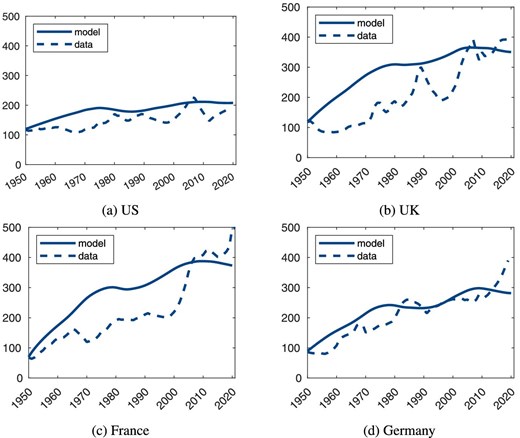
Housing wealth-to-income ratios in US, UK, France, and Germany since 1950 (in %).
The calibrated model captures a significant portion of all four economies’ growth in housing wealth-to-income ratios since the 1950s. Specifically, for the UK, France, and Germany, the model accounts for 84%, 70%, and 63% of the increase in the housing wealth-to-income ratio since 1950, respectively. In the US, the model’s prediction slightly exceeds the actual increase by 20 percentage points toward the end of the observed period.
We intentionally abstract from short-run shocks to keep the model simple and focus on the long run. Despite this intentional abstraction, the model’s predictions align closely with the actual data in the short run, especially for the US and Germany. For the UK and France, the model overestimates the growth of housing wealth in earlier decades, which, especially for the European countries, might be attributed to the absence of specific data like construction sector productivity and other externally calibrated parameters; see Online Appendix B.1.3. For this reason and to streamline the discussion, we will focus on the US for the remaining part of this section.
Figure 3 depicts the evolution of other housing-related variables for the US since 1950, including the house price, rent, residential land price, structure price, and their corresponding quantities. As shown in Figure 3a, the calibrated model closely traces the actual trajectory of the US house price. However, as expected, it does not capture the boom and bust periods related to the financial crisis. Our model also aligns nearly perfectly with the housing rent at the end of the observation period; see Figure 3b. The calibrated model also replicates the mirror-like behavior of residential land and structure prices compared to residential land and structure quantities, as shown in Figures 3c and 3d. Residential land prices grow faster than residential structure prices, and the reverse holds for quantity indices of residential land and structure. Quantitatively, the model tends to underpredict the rise in residential land prices and quantities throughout most of the period. In Section 7.1.2, we demonstrate how a model extension can enhance the quantitative fit for both residential land and structure prices, as well as their respective quantities.
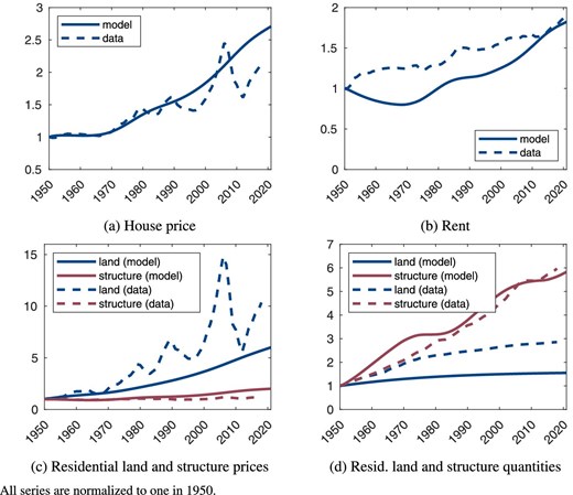
Housing-related prices and quantities since 1950.
6.3. Explaining the Rising Housing Wealth-to-Income Ratio and House Price
Why do the housing wealth-to-income ratio and the house price increase over time? In Section 5, we have identified conditions under which the house price grows in the steady state. However, our analysis reveals that approximately two-thirds of house price growth from 1950 to 2021 is attributable to steady-state growth, while the remaining third stems from additional transitional forces. More importantly, the housing wealth-to-income ratio does not grow in a steady state. This leads us to investigate what exogenous drivers contribute to changes in the house price and housing wealth-to-income ratio during the transition. In technical terms, transitional dynamics arise from initial deviations in capital, developed land, and residential structures—represented by |$K_0$|, |$L^H_0$|, and |$X_0$|—from their respective steady-state values and exogenous changes in population size S, the employment-to-population ratio |$N/S$|, and construction sector productivity |$B^X$|.
Before examining the impact of endogenous state variables, we investigate the influence of exogenous state variables on the housing wealth-to-income ratio and the house price through counterfactual analysis. In this scenario, we hold either S, |$N/S$|, or |$B^X$| constant at their 1950 levels rather than allowing them to evolve according to the baseline calibration depicted in the last panel of Figure 4d. The resulting counterfactual series for the two key outcomes are represented by red lines in the first two panels of Figure 4.24
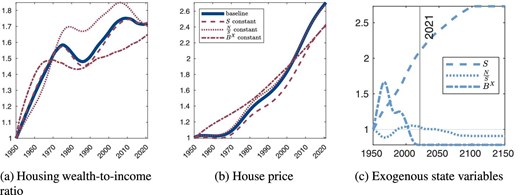
Counterfactual transitions for different exogenous state variables.
Let us first evaluate what happens if population size S counterfactually stays constant instead of increasing as in the baseline scenario. According to Figure 4a, the corresponding red dashed line is very close to the bold blue line. Thus, population growth explains very little of the increase in the housing-wealth-to-income ratio. Intuitively, a rising population size impacts both the numerator—via increased demand for housing—and the denominator—via an expanded labor force—of the housing wealth-to-income ratio, leaving it almost unchanged. In contrast, because of the housing demand effect, the growth in the house price can partly be attributed to an increase in population size, as shown in Figure 4b.
We subsequently investigate the impact of construction sector productivity, which surged in the 1950s and 1960s, declined thereafter, and has recently plateaued. Consequently, both the housing wealth-to-income ratio and the house price would have risen more rapidly early in the transition and more sluggishly later had |$B^X$| remained constant. In summary, both housing metrics would have been marginally lower in recent periods.
Finally, the employment-population ratio first decreased—driven by the increase in female labor force participation and the entrance of baby boomers into the labor market—before starting to decrease from 2010 onward, as is also predicted for the future due to demographic change. The counterfactual scenario of |$N/S$| staying constant leads to a somewhat higher housing wealth-to-income ratio earlier in the transition (by lowering NNP), but overall its development does not explain recent values. It also plays a negligible role for house prices.
Hence, the bulk of the observed increases in the housing wealth-to-income ratio and the house price cannot be attributed to the evolution of the exogenous state variables in the model. Rather, they are driven by the low initial levels of the stock of non-residential capital, |$K_0$|, and residential structure, |$X_0$|, compared to their respective steady-state values, as we explain next.
In Online Appendix D.1, we use impulse response functions to assess the relative contribution of each endogenous state variable to the transitional growth of the two outcome variables. This back-of-the-envelope calculation multiplies the elasticities of a one percent shock to one of the three endogenous state variables with the proportional deviation of the respective state variable from its steady state.
According to our calibration, the initial level of residential structures is below its steady state. This low initial level accounts for 75% of the increase in the housing wealth-to-income ratio.25 A low initial stock of residential structures implies high marginal productivity in housing services production. This leads to substantial residential investment and rapid growth in housing wealth. The low initial level of capital accounts for 16% of the increase in the housing wealth-to-income ratio. This contribution represents a net effect of capital accumulation on the house price and NNP. The low initial level of residential land accounts for the remaining 9%.
We also find that a low initial level of capital implies that the house price increases over time. A low initial level of capital triggers fast capital accumulation, thereby pushing up the house price through rising housing demand and a declining interest rate. Low initial levels of residential structures and land imply that the house price decreases over time. The implied accumulation of residential buildings and residential land dampens house price growth because it is associated with an enlarging housing supply.26
We further corroborate this explanation with two additional observations in the Online Appendix. First, residential investment as a share of GDP has declined in the model and data since 1950, in line with the pronounced US construction boom observed in the 1950s and 1960s. Second, both model and data imply that the aggregate saving rate has declined since 1950.
To summarize, the key driver for the increase in the housing wealth-to-income ratio since 1950 is the accumulation of non-residential capital and residential structures in response to low initial levels of capital and residential structures, relative to their long-run steady state values.27 Our explanation is thus based on both history and the future evolution of exogenous state variables that affect the steady-state level of endogenous state variables.
Thinking beyond the model, the historical component can be thought of as the result of underinvestment during the first half of the 20th century. During WWII, much activity in the US economy was redirected toward the war effort, and investment in residential structures and non-war-related capital was low. Likewise, the Great Depression suppressed private savings and investment. In Continental Europe, the destruction of capital and residential structures during WWII also led to low initial stocks of non-residential capital and residential structures. This interpretation aligns with the observed U-shape in the total wealth-to-income ratio during the 20th century (Piketty and Zucman 2014).28
7. Discussion
In this section, we first discuss further channels that may be important for understanding the surge in house prices and housing wealth: (i) increasing home-ownership rates, (ii) a weak EoS between residential land and structure in housing production, and (iii) declining real interest rates. Second, we comment on two important price relations in our model: between house prices and rents and between residential and non-residential land prices.
7.1. Alternative Explanations for the Surge in House Prices and Housing Wealth
7.1.1. Home-Ownership Revolution
The home-ownership rate has risen over the second half of the 20th century in many countries, including the US, UK, France, and Germany (Kohl 2017). This process is often referred to as home-ownership revolution. A widely held view is that financial liberalization, by relaxing credit constraints, has primarily triggered this evolution (Ortalo-Magne and Rady 2006).29 Provided that the surge in the home-ownership rate, the story goes, pushes the overall demand for housing upwards, this process has contributed to the increase in house prices.30 However, the descriptive empirical picture on the evolution of the aggregate housing expenditure share is ambiguous. Piazzesi and Schneider (2016) argue that the housing expenditure share is fairly stable over time at 19% in the post-war US as implied by data form the US NIPA. Albouy, Ehrlich, and Liu (2016) study also alternative data sources and argue that the housing expenditure share may have increased in the US.
Whether or not the home-ownership revolution has significantly contributed to the surge in house prices appears an open research question. Let us assume that this channel is important. How can this channel be captured by our analysis? Notice that we model all households as renters, but the results do not change if we assume that all households are home owners. We could employ a short-cut to capture an additional demand effect due to the home-ownership revolution by assuming that the expenditure share, which equals |$\theta$| in our model, increases exogenously over time. This would further add to the growing demand for housing and amplify house price growth and the surge in housing wealth. Our supply-side setting, however, is still necessary to generate a plausible increase in house prices and housing wealth such that land prices increase much more than construction cost. Hence, even when studying this potential channel, it is necessary to consider the supply-side features proposed in our model.
7.1.2. CES Technology in Housing Services
A channel that originates from the supply side concerns the role of land in housing services production. Miles and Sefton (2021) argue that the EoS between land and structure is less than one. As the economy grows and the demand for housing increases, the long-run price elasticity of housing supply is relatively low as the fixed factor (land) cannot be easily substituted for by the accumulable factor (structure). The consequence is stronger rent and house price growth compared to the Cobb–Douglas case. We have implicitly assumed an EoS of one in the production function of housing, |$H(X,L^H)$|. We now assume that the production technology for housing services is given by the CES function
where |$\chi \gt 0$| is the EoS between land and structures.
If |$\chi \ne 1$|, a steady-state equilibrium only exists if both X and |$L^H$| grow at the same rates, and it hence has to hold that
This knife-edge restriction implies differential technological progress that is heavily biased toward the non-housing good. We first re-calibrate the model with |$\chi =1$| under this knife-edge condition. To gauge the role of the EoS, we then study how changing |$\chi$| from 1 to a low value of 0.1 in the recalibrated model affects the model outcomes.
The results are shown in Online Appendix Table D.1 in the Online Appendix. To summarize, weaker substitutability of structure and land results in higher growth differences in prices and quantities of land and structure. Hence, the model fits stylized facts 2 and 3 quantitatively better. This modification also generates an increasing land share in housing wealth—stylized Fact 5—which the baseline model cannot. However, this extension requires imposing a knife-edge condition on differential technological growth to restore the existence of a steady state.
7.1.3. Declining Real Interest Rate
Rachel and Summers (2019) show that the real interest rate has been trending downward since the early 1980s.31 Viewing houses as assets suggests that the house price is given by the PDV of future rental yields. A decline in the real interest rate over time then implies that the house price increases as time goes by. This mechanical discounting effect operates as long as the discount factor declines. Miles and Monro (2021) argue that the rise in house prices (relative to incomes) between 1985 and 2018 can be more than accounted for by the substantial decline in the real risk-free interest rate observed over that period.32 Because the interest rate is endogenous in our model, it is impossible to ask how its change affects prices. However, the endogenous dynamics of the interest rate are in line with the empirical observation of declining interest rates. The real interest rates declines because capital starts below its steady state and accumulates over time, reducing the marginal product of capital and hence the interest rate. Our explanation for rising house prices is therefore in line with the empirical trend in the real interest rate.
7.2. Other Relevant Price Variables
7.2.1. Price-to-Rent Ratio
Can the price-to-rent ratio change over time in our model, and if yes, why? The no-arbitrage condition (20), together with an appropriate boundary condition excluding asset price bubbles, implies that the house price, at any point in time, equals the PDV of current and future rents. All the variation of house prices comes from the variation of current or future rents and the discount rate used to price these cash flows. In the steady state, the discount rate is constant, and the house price grows at the same rate as the rent, implying that the price-to-rent ratio is constant; see Table 2. Along the transition, however, the price-to-rent ratio can change over time, even though we abstract from frictions or bubbles. The price-to-rent ratio can change if the discount rate or expected future rents change in a way that does not translate into house-price changes by the same magnitude. To what extent is this implication of the model consistent with the empirical evidence on house prices, rents, and interest rates?
Focusing on short-run volatility, Shiller (2016) argued that the variation of current or future rents and the discount rate could not explain the variation in house prices.33 Campbell et al. (2009) provide a decomposition of expected future returns to housing assets to understand the movement of the rent-price ratio at semi-annual frequencies. They argue that the volatility in price-to-rent ratios is closely related to changes in expected future housing premia. Our model is not designed to investigate the short-run volatility of asset prices.
Since the 1950s, house prices have increased stronger than rents in most industrialized countries (Jordà et al. 2019).34 Our calibrated model produces price-to-rent ratios that are consistent with this empirical observation. Online Appendix Figure D.4 in the Online Appendix shows the price-to-rent ratio and the corresponding empirical series for the US, UK, France, and Germany. In the transition, the price-to-rent ratio increases over time, consistent with empirical evidence. This pattern is largely, although not exclusively, driven by the already discussed decline in the real interest rate that pushes house prices up over time.35 Hence, without resorting to financial frictions or bubbles, our model can plausibly replicate the increase in the price-to-rent ratio over the last seven decades.
7.2.2. Residential and non-Residential Land Prices
What is the relationship between the price of residential land (|$P_t^{LH}$|) and the price of non-residential land (|$P_t^{LY}$|) in our calibrated model? For all economies considered, the initial price of residential land exceeds the initial price of non-residential land (|$P_{1950}^{LH} \ge P_{1950}^{LY}$|). This price difference provides the incentive for a reallocation of land toward housing. Moreover, both prices coincide in the steady state (|$\widetilde{P}_t^{LH}=\widetilde{P}_t^{LY}$|), implying a stationary land allocation. That is, the price of non-residential land grows faster along the transition than the price of residential land. This implication can be expected to carry over to residential house prices and commercial real estate prices.36 Data on the long-term trends of house prices (Knoll, Schularick, and Steger 2017) and commercial real estate prices in the US (Board of Governors of the Federal Reserve System (US) 2023) indicate a pronounced decline of the house price to commercial real estate price ratio. However, our model does not explicitly capture commercial real estate as an asset. Our focus is on private housing wealth that does not comprise real estate property.37
8. Conclusion
The housing wealth-to-income ratio and house prices have increased in the US, the UK, France, and Germany since 1950. Decomposing housing wealth into the value of residential structure and the value of residential land indicates that the land share in housing wealth has significantly grown over time in these economies. Further decomposing the values of land and structure into price and quantity components reveals a mirror-like pattern: The price of residential land increased enormously, while its quantity remained relatively stable. The opposite holds for the reproducible factor—structures. Its quantity increased strongly and its price only modestly.
Motivated by these observations, we propose a novel model for studying the house price and housing wealth-to-income ratio in the long run. The employed Ramsey growth model comprises a numeraire sector and a housing sector. Both sectors experience different technological progress and operate under different land intensities in equilibrium. The overall land supply is fixed and the sectoral land allocation is endogenous. Exogenous drivers of economic growth are technological change, population growth, and a change in the employment-population ratio over time. We also investigate the role of initial values of capital, residential structures, and residential land use.
According to our model, two fundamental forces drive the long-run house price growth. First, the land intensity in the housing sector has to be larger than in the non-housing sector. Under this condition, (symmetric) technological progress leads to rising house prices. Second, house prices grow in the long run if technological progress in the construction sector lags behind technological progress in the rest of the economy. We argue that both conditions are empirically plausible.
While the house price and housing wealth can increase in the steady state and do so in the calibrated model, the housing wealth-to-income ratio is constant in the steady state. Explaining a rising housing wealth-to-income ratio requires studying transitions. The calibrated model replicates most of the observed increase in the housing wealth-to-income ratio since the 1950s in the considered economies. The analysis is also consistent with a significant increase in the number of residential buildings during the latter half of the 20th century, alongside a relatively modest increase in the quantity of residential land. The expansion in the stock of residential structures has directly contributed to the surge in housing wealth. Moreover, and in contrast to the evolution of quantities, our model suggests that land prices grow faster than structure prices, consistent with the empirical evidence. Intuitively, rising housing demand, driven by the exogenous forces of the model, meets an inelastic supply of residential land and an elastic supply of residential structures. Finally, related to an endogenously declining interest rate over time, the model also explains the empirically observed increase in the house price-to-rent ratio.
Acknowledgments
We thank the editor, Guido Lorenzoni, an anonymous reviewer as well as Christian Bayer, Gilles Duranton, Josef Falkinger, Jan Grobovsek, Andreas Irmen, Markus Knell, Winfried Koeniger, Chris Papageorgiou, Michael Peters, Thomas Piketty, Pietro Reichlin, Moritz Schularick, Sjak Smulders, Etienne Wasmer, and seminar participants in Bonn, Göttingen, Linnaeus University, Mainz, Munich (LMU), Münster, at the IMF, Norges Bank, Paris School of Economics, Riksbank, Sciences Po Paris, AMES in Kyoto, DEGIT in Nottingham, ESEM in Geneva, Macroeconomic Council of the VfS Meeting in Munich, VfS Meeting in Augsburg, ESSIM in Tarragona, and SED in Edinburgh for helpful comments and suggestions. We are also grateful to Moritz Schularick, Luis Bauluz, and Filip Novokmet for sharing their data on housing wealth and to Hannah Ventz for excellent research assistance.
Notes
The editor in charge of this paper was Guido Lorenzoni.
Appendix A: Data for Figure 1 and Table 1
Total wealth—to be precise, nominal net private wealth—for France, Germany, the UK, and the US, from 1950 to 2021, is an updated series from Piketty and Zucman (2014) available at www.wid.world. US nominal housing wealth and US nominal residential structure wealth is from the updated online appendix of Davis and Heathcote (2007), available at www.aei.org/historical-land-price-indicators/. The data contain observations from 1950 to 2018. We use the quarterly data from 1975 onward because it has a higher quality and the annual data for earlier periods. Data on nominal housing wealth and nominal residential structure wealth for the other three economies are provided by Moritz Schularick, Luis Bauluz, and Filip Novokmet.38 Nominal residential structure wealth is available from 1950 to 2021 in all three economies, while nominal housing wealth is available from 1950 to 2019 in the UK and Germany and from 1950 to 2021 in France. Non-housing wealth is obtained by subtracting housing wealth from total wealth. Similarly, residential land wealth is obtained by subtracting residential structure wealth from housing wealth.39 For France and Germany, the estimates of the value of residential structures are too large for early years, resulting in negative residential land values. Therefore, we consider residential structure and land wealth for Germany and France from 1960 onwards. We always consider gross housing wealth as opposed to net housing wealth, where mortgage debt is subtracted from gross housing wealth. Nominal NNP is also from www.wid.world for all four economies from 1950 to 2021. Wealth-to-income ratios are obtained by dividing nominal wealth series by NNP. The share of residential land wealth in housing wealth is obtained by dividing residential land wealth by housing wealth.
Data on aggregate nominal house prices, residential land prices, and residential structure prices is based Davis and Heathcote (2007) and obtained at www.aei.org/historical-land-price-indicators/ for the US, from 1950 to 2018. We obtain real prices by dividing nominal prices by the CPI that is the series “CPIAUCNS” as given by https://fred.stlouisfed.org/. House prices for France, UK, and Germany are from Knoll, Schularick, and Steger (2017), obtained in an updated version at http://www.macrohistory.net/. For France and UK, observations are available from 1950 to 2020 and for Germany from 1962 to 2020. Residential land prices and residential structure prices for France, UK, and Germany are from Knoll, Schularick, and Steger (2017), as provided in their online appendix at the journal’s webpage and the respective CPI’s are from http://www.macrohistory.net/. For France and UK, observations are available from 1950 to 2012 and for Germany from 1962 to 2012.
We compute the quantity indices for housing, residential land, and residential structures by dividing the respective value index by the respective price index, that is, |$ \text{quantity index } = \frac{ \text{value index} }{ \text{ price index} }$|.
Lastly, the nominal rent as well as the interest rate for all four economies from 1950 to 2020 are from Jordà et al. (2019) and downloaded at http://www.macrohistory.net/. The real rent is obtained by multiplying the housing rental yield with the nominal house price and dividing by the CPI. The real interest rate is the portfolio-weighted rate of return on total wealth.
Appendix B: Calibration
We calibrate the model to all four economies—US, UK, France, and Germany—separately at annual frequency since 1950. Due to better data availability and quality, we focus on the US first, before turning to the other three economies in Appendix B.1.3.
B.1 Calibration for the US
B.1.1. Parameters Calibrated from External Sources
We calibrate the set of parameters |$\lbrace \theta , \sigma , \delta ^K, \delta ^X, \beta , \lbrace S_t, N_t, B_t^X\rbrace _{t=0}^\infty , g^X \rbrace$| without solving the model numerically. Table B.1 summarizes the calibration for the US. The preference parameter |$\theta$| equals the aggregate share of housing expenditures in total consumption expenditures. According to the Consumer Expenditure Survey, this value is relatively stable at an average of 19% since 1950 (U.S. Bureau of Labor Statistics 2016).40 The IES in composite consumption, |$C^{1-\theta }S^\theta$|, is |$1/\sigma$|. In a meta-study, Havránek (2015) shows that mean-estimates based on micro-studies and asset holders are in the range of 0.3–0.4. Best et al. (2020) estimate an aggregate IES of 0.1 using quasi-experimental variation in UK interest rates. We, therefore, set |$\sigma = 10/3$| to match the lower bound of 0.3 from Havránek (2015). The depreciation rates of capital and structures are set to annual values of 5.6% (Davis and Heathcote 2005) and 1.5% (Hornstein 2009, p. 13), respectively.41
Parameter calibration from external sources, US.
| Parameter | Value | Explanation/Target |
|---|---|---|
| |$\theta$| | 0.19 | Housing expenditure share |
| |$\sigma$| | |$10/3$| | IES |
| |$\delta ^K$| | |$\ln (1+0.056)$| | Capital depreciation rate |
| |$\delta ^X$| | |$\ln (1+0.015)$| | Structure depreciation rate |
| |$\beta$| | 0.613 | Labor income share in Y sector |
| |$\lbrace S_t, N_t\rbrace _{t=0}^\infty$| | From UN (2019), medium scenario | Population and labor dynamics |
| |$\lbrace B^X_t\rbrace _{t=0}^\infty$| | From Foerster et al. (2022), 1950–2018, constant thereafter | Construction sector productivity |
The parameter |$\beta$| equals the labor income share of the non-housing sector, |$ ( w L^{Y})/Y$|. We use data from the US Bureau of Economic Analysis (BEA) that is available from 1997 to 2018.42 The non-housing labor share is relatively stable over time, declining only by 1.2 percentage points since 2008. The average is 61.3% and we hence set |$\beta = 0.613$|. The exogenous population and labor supply sequences, |$\lbrace S_{t}, N_{t}\rbrace _{t=0}^{\infty}$|, are constructed from UN (2019), medium scenario, for 1950–2100, assuming initial levels (for 1950), |$S_0=N_0=1$|. We assume that both remain constant after 2100. Following Martin (2005), we are not using total hours worked to calibrate time path |$\lbrace N_t\rbrace _{t=0}^{\infty}$| because (i) this series fluctuates strongly over the business cycle and (ii) predictions up until 2100 are imprecise. Instead, we use the empirical ratio of the working-age population (25–64) to the total population and multiply it by the calibrated value |$S_t$| to obtain |$N_t$|. This value is better predictable than total hours, and we capture the future demographic change to the full extent. Lastly, we obtain |$ \lbrace B_t^X \rbrace _{t=0}^{68}$| from filtered TFP growth rate in the construction sector as calculated by Foerster et al. (2022, Fig. 4, data from journal webpage) for 1950–2018, normalizing |$B_0^X=1$|. (We also normalize |$B_0^Y=1$|.) As trend growth of construction sector productivity has been almost zero for recent years, we assume that |$B_t^X = B_{68}^X$| for |$t \ge 68$| and set the long-run growth rate in the construction sector to zero, |$g^X=0$|. The exogenous, time-variant variables |$S_t, N_t/S_t$|, and |$B^X_t$| are visualized in Figure 4c.
B.1.2. Parameters Calibrated Jointly Inside the Model
The remaining six parameters |$ \alpha , \gamma , \eta , \rho , \xi$|, and |$g^Y$| as well as the three initial states |$K_0, L^H_0$|, and |$X_0$| are calibrated by solving the transition many times for different parameter values until the model matches a set of nine empirical moments. Although all parameters jointly determine the theoretical moments, we explain in the following each parameter in combination with the moment that it most strongly affects.
The time preference rate |$\rho$| is chosen to match the level of the total wealth-to-income ratio of 3.6 (see Section 3) at the beginning of the transition in 1950. Similarly, we set the initial capital stock, |$K_0$|, to match the housing wealth-to-income ratio of 1.2 in 1950. The technology growth rate of the non-housing sector, |$g^Y$|, is set to match the average annual growth rate of 2.6% of US national income between 1950 and 2021. These three moments imply that we match the levels of the total wealth-to-income ratio and the housing wealth-to-income ratio, as well as the growth in their denominator. However, the dynamics in total wealth and housing wealth are not targeted by our calibration. By matching the growth in national income, we rule out that the model replicates wealth-to-income ratio increases by implausible income dynamics.
The parameter |$\gamma$| is the output elasticity of structures in the production of houses. The larger |$\gamma$|, the more relevant structures are, and the less relevant land is for the production of houses. This parameter strongly affects the share of residential land wealth in total housing wealth, the land share. The smaller |$\gamma$| is, the larger the land share. As shown in Figure 1, the land share has increased since 1950. To adequately capture the relevance of land in the production of houses, we choose |$\gamma$| such that the steady-state land share equals the most recent empirical value of 35.2% in 2018. We discuss the land share dynamics in detail in Section 7.1.2.
Similarly, the parameter |$\eta$| is the output elasticity of materials in the construction sector. The smaller |$\eta$| is, the smaller the demand for materials and the larger the demand for labor. We, hence, set |$\eta$| to match the long-run employment share in the residential construction sector of 2.5%.43 We target the long-run value of the employment share in residential construction because data are only available for more recent periods but not for 1950.
The initial stock of residential structures, |$X_0$|, is set to match the share of residential investment in GDP of 5.6% in 1950, as taken from Federal Reserve Economic Data. In the model, residential investment is defined as follows:
We included investment in residential land because the empirical data does not differentiate between investment into land and structures. The output elasticity of capital in the numeraire sector, |$\alpha$|, is set to match the net income share of non-developed land, |$R^{LY} N^Y / NNP$| of 10% in 1950.44 This is related to |$\alpha$| because the income share of non-developed land in output of the numeraire sector is given by |$1-\alpha -\beta$|. The parameter |$\xi$| governs the speed of convergence in developed land, |$L^H$|. We set it such that we match the half-life in the transition of residential land of 20.6 years.45 Lastly, the initial stock of residential land, |$L^H_0$|, is chosen such that we match the average annual growth rate of residential structures relative to residential land of 1.1% between 1950 and 2018, as implied by Table 1. The targeted moments are shown in Table B.2 and the resulting parameter values in Table B.3.
Targeted data and model moments, US.
| Moment | Data | Model |
|---|---|---|
| 1 |$\frac{W}{NNP}$|, in 1950 | 3.6 | 3.6 |
| 2 |$NNP$|, average annual growth rate in % | 2.6 | 2.6 |
| 3 |$\frac{P^H H }{NNP}$|, in 1950 | 1.2 | 1.2 |
| 4 |$\frac{P^{LH} L^H}{P^H H} \times 100$|, long run | 35.2 | 35.2 |
| 5 |$\frac{N^X}{N} \times 100$|, long run | 2.5 | 2.5 |
| 6 |$\frac{I^H}{GDP} \times 100$|, in 1950 | 5.6 | 5.6 |
| 7 |$\frac{R^{LY} L^Y}{NNP} \times 100$|, in 1950 | 10.0 | 10.0 |
| 8 Half-life of |$L^H$|, in years | 20.6 | 20.6 |
| 9 |$\frac{X}{L^H}$|, average annual growth rate in % | 1.1 | 1.1 |
See text for data sources.
Endogenously calibrated parameters, US.
| # | Parameter | Explanation | Value |
|---|---|---|---|
| 1 | |$\rho$| | Time preference rate | 0.051 |
| 2 | |$g^Y$| | Labor efficiency growth in numeraire sector | 0.019 |
| 3 | |$K_0/K^{*}$| | Initial capital stock | 0.321 |
| 4 | |$\gamma$| | Structures’ elasticity in H | 0.709 |
| 5 | |$\eta$| | Materials’ elasticity in |$I^X$| | 0.485 |
| 6 | |$X_0/X^{*}$| | Initial stock of residential structures | 0.279 |
| 7 | |$\alpha$| | Capital elasticity in Y | 0.274 |
| 8 | |$\xi$| | Intensity of convex adjustment cost in land development | 332.15 |
| 9 | |$L^H_0/{L^H}^{*}$| | Initial stock of residential land | 0.626 |
Initial states, |$K_0, L^H_0, X_0$|, are expressed relative to their respective final steady-state values, denoted by superscript |$^{*}$|.
B.1.3. Calibration for UK, France, and Germany
The parameters |$\alpha$|, |$\beta$|, |$\delta ^K$|, |$\delta ^X$|, |$\sigma$|, and |$\xi$| are set to the same values as for the US. Because we lack evidence for the productivity dynamics in the construction sector for UK, France and Germany, we also assume that the time series for |$B_t^X$| is the same as in the US; see Table B.2. We set the housing expenditure share, |$\theta$|, to 17%, 22%, and 27% for the UK, France, and Germany, respectively.46 The exogenous population and employment series are all taken from UN (2019), as for the US. The remaining set of parameters |$\lbrace \rho , \gamma , \eta , g^Y, K_0, L^H_0, X_0\rbrace$| is calibrated by matching a corresponding subset of the moments we target for the US. Most data moments are from the data explained in Section 3 and Appendix A, except for the following. Residential investment, |$I^H$|, is from the UK ONS and the OECD Database for France and Germany. Available data starts in 1962 in the UK and 1970 in France and Germany. To obtain the same time spans across all four economies, we assume that |$I^H / GDP$| was similar in 1950 as in 1962 or 1970, respectively. Alternatively, one could start the simulation in 1962 for the UK and in 1970 for Germany and France. The share of employment in the residential construction sector, |$N^X/N$|, is calculated by multiplying two variables: the employment share in the construction sector and the share of value-added of the residential construction sector in the entire construction sector. The data are obtained from national statistical agencies and Eurostat. The moments we match and the resulting parameter values are shown in Table B.4.
Calibration for UK, France, and Germany.
| (A) Endogenous parameters | |||||||
|---|---|---|---|---|---|---|---|
| Value | |||||||
| # | Parameter | Explanation | UK | FR | DE | ||
| 1 | |$\rho$| | Time preference rate | 0.004 | 0.031 | 0.042 | ||
| 2 | |$g^Y$| | Technical growth in numeraire sector | 0.023 | 0.023 | 0.031 | ||
| 3 | |$K_0/K$| | Initial capital stock (share of final) | 0.315 | 0.152 | 0.376 | ||
| 4 | |$\gamma$| | Structures’ elasticity in H | 0.516 | 0.492 | 0.586 | ||
| 5 | |$\eta$| | Materials’ elasticity in |$I^X$| | 0.593 | 0.104 | 0.306 | ||
| 6 | |$X_0/X$| | Initial stock of residential structures | 0.280 | 0.145 | 0.429 | ||
| 7 | |$L^H_0/L^H$| | Initial stock of residential land | 0.586 | 0.547 | 0.386 | ||
| (B) Targets | |||||||
| UK | FR | DE | |||||
| Moment | Data | Model | Data | Model | Data | Model | |
| 1 | |$\frac{W}{NNP}$|, in 1950 | 3.9 | 3.9 | 1.8 | 1.8 | 2.0 | 2.0 |
| 2 | |$NNP$|, average annual | 2.4 | 2.4 | 2.8 | 2.8 | 3.2 | 3.2 |
| growth rate in % | |||||||
| 3 | |$\frac{P^H H }{NNP}$|, in 1950 | 1.2 | 1.2 | 0.7 | 0.7 | 0.9 | 0.9 |
| 4 | |$\frac{P^{LH} L^H}{P^H H} \times 100$|, long run | 61.6 | 61.6 | 54.9 | 54.9 | 45.7 | 45.7 |
| 5 | |$\frac{N^X}{N} \times 100$|, long run | 2.1 | 2.1 | 3.4 | 3.4 | 4.1 | 4.1 |
| 6 | |$\frac{I^H}{GDP} \times 100$|, in 1950 | 5.0 | 5.0 | 9.4 | 9.4 | 7.3 | 7.3 |
| 7 | |$\frac{X}{L^H}$|, average annual | 1.2 | 1.2 | 2.4 | 2.4 | 0.5 | 0.5 |
| growth rate in % | |||||||
Initial states, |$K_0, L^H_0, X_0$|, are expressed relative to their respective final steady-state values (normalized). Data sources are described in the text.
Footnotes
The data behind these numbers and further stylized facts are presented in Section 3.
The mortgage-to-GDP ratio is given by leverage ratio |$\times$| housing wealth-to-income ratio. A rising housing wealth-to-income ratio raises, given a constant leverage ratio, the mortgage-to-GDP ratio.
The housing capital income share is given by housing yield |$\times$| housing wealth-to-income ratio.
This is not an implication specific to our model but a common implication of macroeconomic models. For instance, in a one-sectoral economy, it intuitively results from the assumption of constant returns to scale in production, which implies that the capital-output ratio is constant. More generally, a time-varying wealth-to-income ratio can either be explained as a sequence of steady states (Piketty and Zucman 2015; Borri and Reichlin 2018) or a transition toward a given steady state (Gennaioli, Shleifer, and Vishny 2014)
The period 1940–1975 is known as the era of mass suburbanization, during which new residential areas evolved at the boundaries of US cities (Nechyba and Walsh 2004).
One of the first economists to be concerned about the long-run consequences of the fixed factor land was Ricardo (1817). He argues that economic growth benefits landlords as the owners of the fixed factor disproportionately; see also Piketty (2014). While Ricardo was mainly concerned with agricultural land and the production of corn to feed a growing population, societies in modern times are confronted with the need for residential investments to meet the increasing demand for housing services under the constraint of a fixed supply of land. Nichols (1970) includes a productive factor, which is in fixed supply (land), into a Solow model. He shows that the land price increases at the same growth rate as output in a steady state.
This predominance of housing wealth growth is emphasized by Bonnet et al. (2019).
These contributions focus on prices and do not discuss quantities and wealth.
Divide both sides of equation (1) by the housing wealth-to-income ratio to obtain |$1 = \text{value of structures} / \text{housing wealth} + \text{value of land} / \text{housing wealth}$|, where the second fraction on the right-hand side is the share of land wealth in total housing wealth.
Throughout, we use the terms numeraire sector and non-housing sector interchangeably.
We suppress the time index t whenever no confusion arises.
Our separate modeling of labor supply and population size to capture an exogenous demographic structure in an infinitely lived household economy follows Martin (2005). We are thankful to an anonymous referee for the suggestion.
We model all households as renters, but the results do not change if we assume owner-occupied housing.
We explain the different economic activities involved in the supply side of the housing sector as undertaken by three different types of firms, but other institutional arrangements are equivalent. For example, one can equivalently assume that one firm sector engages in all three activities simultaneously.
If |$P^{LH}$| were larger than |$P^{LY}$|, firms would transfer as much land as possible from the numeraire to the housing sector, demanding more and more |$L^Y$| and supplying more and more |$L^H$|. The price of land in the numeraire sector would increase, and the price of residential land would decrease until they are equal. The same reasoning applies for |$P^{LH} \lt P^{LY}$|.
Our specification of the adjustment cost function |${{N}}^{L}\,(\cdot )$| has the property that |$N^{L}\, \gt\, {0} $| for |$I^{L} \gtrless {0}$| and therefore, an interior solution also exists for negative investment in residential land.
If the rate of return on an asset deviated from r, households would demand either zero or an infinite amount of the asset and markets would not clear.
See, for instance, Davis and Heathcote (2005), Favilukis, Ludvigson, and Nieuwerburgh (2017), Greenwald and Guren (2019), Kaplan, Mitman, and Violante (2020). A notable exception is Herkenhoff, Ohanian, and Prescott (2018), who assume a fixed supply of land but abstract from differential technological growth, a separate construction sector, and adjustment costs in land reallocation.
This mechanism is related to the Findlay–Grubert theorem that considers the output and price effects of differential technological change.
Combes, Duranton, and Gobillon (2021) focus on newly built single-family homes in France and estimate |$\gamma =0.65$| that is close to our calibrated value of |$\gamma =0.49$| for all buildings. |$\psi ^{H} \gt \psi ^{Y}$| well holds also for |$\gamma =0.65$|. Assuming constant returns to scale, Epple, Gordon, and Sieg (2010) find an output elasticity of land in the US region Allegheny County, Pennsylvania, of 0.14, suggesting |$\gamma =0.86$|. If we take this value for the US as a whole, we see that |$\psi ^{H} \gt \psi ^{Y}$| if |$\eta \gt 0.19$|. Our calibration strategy suggests |$\eta =0.49$|. Although direct estimates of |$\eta$| are not available, to our knowledge, the evidence suggests that the construction sector is the most material-intensive sector in the economy. The residential building sector accounts for 30%–50% of total material consumption in the economy (Marinova et al. 2020). In OECD countries, construction minerals alone (e.g., sand, gravel, crushed natural stone, brick clays, gypsum) accounted for 36% of material consumption in the year 2010 (OECD 2015). This is remarkable, given that, on average, over the period 1950–2018, the construction sector only generated about 5% of total value-added in the US (Foerster et al. 2022, Table 2).
In a one-sectoral economy, it intuitively results from the assumption of a constant returns-to-scale production function, which implies that the capital-output ratio is constant.
The baseline and counterfactual series begin at differing levels in perfect foresight equilibrium. To emphasize changes over time, we normalize both series to unity in 1950.
Recall that the growth in the housing wealth-to-income ratio results entirely from transitional dynamics.
Recall that only one-third of house price growth is attributed to transitional dynamics. The numbers of the decomposition of this transitional growth are the following. Capital accounts for 152%, residential buildings for -38%, and residential land for the remaining -15%.
Incontrast, house price growth can largely be explained by the forces also at play in steady state equilibrium.
The Marshall plan may also have contributed to the post-war reconstruction of European economies. However, as argued by leading economic historians, transfers for housing and capital via the Marshall Plan were only of minor quantitative importance, albeit the Marshall Plan fostered financial stability and market orientation of European economies (Eichengreen and Uzan 1992; DeLong and Eichengreen 1993). See Online Appendix Section D.5 for a brief discussion.
Jordà, Schularick, and Taylor (2016) stress that banks and households have been heavily leveraging up through mortgages in the second half of the 20th century. Mortgage credit on the balance sheets of banks has been the driving force behind the increasing financialization of advanced economies.
It is not clear that an increase in the home-ownership rate raises the aggregate demand for housing since the demand for owner-occupied housing increases, and the demand for rental housing decreases when renters become owners. For the same reason, Kaplan, Mitman, and Violante (2020) find that credit relaxation does not result in a meaningful increase in aggregate demand for housing and, hence, cannot explain the housing boom.
They focus on average yields on long-maturity inflation-protected government securities in the G7, excluding Italy. For alternative measures on the long-term real interest rate and long-term data series; see also Jordà et al. (2019).
They focus on the UK, where the surge in house prices has been especially pronounced. Their main results, they argue, apply to other G7 economies as well.
Shiller (2016) employs data at daily, monthly, quarterly, semi-annual, and annual frequencies.
Miles and Monro (2021) argue that the decline in the real interest rate drives 2/3 of the house price growth in the UK.
The growth rate of house prices differs from the growth rate of residential land only by the growth rate of real construction costs, being low historically, times the share of residential structure in housing value (Knoll, Schularick, and Steger 2017). Furthermore, production cost in residential and commercial construction can be expected to evolve synchronously.
In national wealth accounting, commercial real estate property is part of the value of corporations (Piketty and Zucman, 2014, III.A. Concepts and Definitions).
Housing wealth for Germany is based on Albers, Bartels, and Schularick (2022). Housing wealth for France and the UK is based on Piketty and Zucman (2014) and updated by Bauluz et al. (2023). Data on the value of residential structures and land were collected for Bauluz, Novokmet, and Schularick (2022).
Direct measures of residential land wealth at the aggregate level are very sparse and nonexistent for earlier periods. See Albouy, Ehrlich, and Shin (2018) for a recent paper on this issue. The authors provide the first direct measures of residential land wealth for the US starting in 2005.
See also Piazzesi and Schneider (2016, Section 2.1).
We use the components of value added by industry from https://apps.bea.gov/iTable/iTable.cfm?ReqID=51?step=1, accessed on March 8, 2020.
The employment share in residential construction is obtained by multiplying the employment share in the overall construction sector with the output share of residential construction in total construction. The data is from the National Association of Home Builders at https://www.nahbclassic.org/generic.aspx?sectionID=734&genericContentID=261286 and http://admin.nahb.org/generic.aspx?sectionID=734&genericContentID=178434&channelID=311 and was accessed on Dec 16 2019. It is very stable since 2010 at a value of 2.5%.
The data is taken from Rognlie (2015, Fig. 11).
The data is from each country’s national accounts as documented in our companion paper Grossmann et al. (2021). There we assume non-homothetic preferences and study distributional effects.
