


Abstract
Policymakers ‘imperfect knowledge about firms’ abatement costs leads to inefficient regulation, reducing the welfare gains from carbon markets around the world. We introduce a “smart” cap and trade system that eliminates these costs. This cap responds endogenously to technology or macroeconomic shocks, relying on the market price of certificates to aggregate information. It allows policy makers to modify existing institutions to achieve more efficient emissions reductions. The paper also shows that the slow diffusion of technology innovations typically makes the optimal carbon price a much steeper function of emissions than suggested by the Social Cost of Carbon.
A set of Teaching Slides to accompany this article is available online as Supplementary Data.
1. Introduction
Forty-seven national jurisdictions regulate greenhouse gas (GHG) emissions using either a cap and trade system or a tax (World Bank 2022). Following the Paris Climate Agreement, 88 countries have considered using these instruments.1 At 2022 carbon prices, the European Emissions Trading System (ETS) has an annual market value of around 150 billion USD, more than double its 2021 value. High price fluctuations have plagued most cap and trade systems, leaving major mitigation opportunities on the table at times of low prices and asking firms to mitigate at much higher prices. The high cost of reducing GHG emissions, and the potentially enormous costs of failing to deal with the climate problem, make it important to use efficient policies. We address the inefficiencies triggered by asymmetric information between firms and the regulator: each firm knows its own abatement costs; the regulator does not know even the aggregate abatement costs.2
We propose a “smart” cap that eliminates the welfare costs of asymmetric information. A market for emissions certificates aggregates and reveals information about prevailing abatement technologies. The “smart” nature of the cap ensures that the endogenous equilibrium price corrects the aggregate emissions externality. Under this smart cap, the regulator auctions or gives away certificates at the beginning of each compliance period, and simultaneously announces a “conversion function”. This function specifies the number of allowable units of emissions per certificate as a function of the equilibrium certificate price. We show how to design this conversion function to achieve the first best emissions price, even under asymmetric information. Under a smart cap, the certificate market aggregates the relevant information without the need of tailored incentive schemes or information revelation mechanisms.
In a static setting, the optimal policy steers the certificate price along the marginal damage (MD) curve. In the climate context, these MDs correspond to the discounted future damages from releasing one ton of carbon dioxide (CO|$_2$|) today; they are referred to as the social cost of carbon (SCC). It is generally accepted that this SCC curve, as a function of emissions, is relatively flat. In the static setting, Weitzman (1974) shows that a relatively flat MD curve favors a high price elasticity of optimal emissions. A carbon tax, but not a cap and trade system, produces such a high elasticity of emissions supply. Weitzman (2020) conjectures that “For example in the case of CO|$_2$|, because the [SCC] curve within a regulatory period is very flat [...] the theory strongly advises a fixed price as the optimal regulatory instrument.” We show that the common reasoning that the SCC determines the optimal price elasticity of emissions supply is generally incorrect in a dynamic setting.
We explain the flaw in this reasoning using the important example of technological innovations that reduce firms’ abatement costs. A cost-reducing innovation today also lowers future abatement costs, thereby reducing future CO|$_2$| emissions, future CO|$_2$| concentrations, future damages and, thus, today’s SCC. As a result, an innovation that reduces today’s abatement costs also affects the marginal cost of climate change. Using parallel reasoning, a smaller-than-expected technological innovation implies higher climate costs from a unit of current emissions. As a result, emissions should generally be less responsive to persistent shocks than the SCC would suggest. This insight concerning the emissions response to persistent shocks affects not only optimal policy in general but also affects the choice between the common second-best policy instruments. For example, it is widely believed that, because the slope of the SCC is small, taxes provide a more efficient instrument to control emissions than ordinary cap and trade systems. An accompanying paper shows that our finding also challenges this commonly held belief (Karp and Traeger 2024).
We develop a simple analytically tractable stochastic integrated assessment model to quantify our findings. The model connects stochastic innovation affecting firms’ abatement decisions with the endogenous cost of climate change. We derive the corresponding global smart cap, as well as the corresponding nonlinear tax. We show how the shock-sensitivity of these first-best policy instruments differs from that of the SCC curve. In general, our reasoning applies to all shocks affecting firms’ abatement decisions. Given the importance of the green transition, we focus on the asymmetric information generated by technological innovation, using a tractable model of technology diffusion. We show that efficient mitigation policies are sensitive to the speed of technology diffusion. A regression of emissions on green patents suggests moderately slow diffusion. Slow diffusion increases the slope differences between the SCC (MDs) and the optimal emissions supply curve; optimal emissions and, thus, the first-best smart cap are less responsive to price shocks under slow technology diffusion.
The smart cap is a smooth first-best improvement over hybrid trading systems that add a price floor and ceiling to a standard cap and trade system (Roberts and Spence 1976; Weitzman 1978; Pizer 2002; Hepburn 2006; Fell and Morgenstern 2010; Grüll and Taschini 2011; Fell et al. 2012). In the hybrid system, partly implemented in California, the policy maker commits to buying and selling certificates to keep the abatement cost within a pre-defined price window, making it effectively a tax when the price reaches these boundaries. The smart cap smoothly responds to price changes, eliminating the need for a regulator to buy or sell permits to maintain the price floor or ceiling.
Many papers discuss emissions regulation with asymmetric information for flow pollutants, that is, pollutants that do not cause damages beyond the period in which they are emitted.3 Requate and Unold (2001) explain how the issuance of options on emissions certificates implements a step function approximation to the MD curve. Newell, Pizer, and Zhang (2005) show how a committed agency can manage allowances to use a standard cap for direct price control. Taking this idea a step further, Kollenberg and Taschini (2016) show that an appropriate management of banking reserves can transform a standard cap with banking and borrowing into a hybrid mechanism that continuously interpolates between a standard cap and a standard tax. Pizer and Prest (2020) note that with banking and borrowing, adjustment of the intertemporal exchange rates enables the regulator to achieve the first best, provided that all uncertainty is resolved in the last period.4
It is widely understood that policies should be conditioned on available information (Ellerman and Wing 2003; Jotzo and Pezzey 2007; Newell and Pizer 2008; Doda 2016). Burtraw et al. (2020) note that a policy that conditions the current quota allocation on previous prices increases welfare relative to a standard cap or tax. The absence of such conditioning is less harmful under a smart cap because of its automatic adjustment to the price of certificates. Nevertheless, we still recommend explicit conditioning on observables in order to tailor the smart cap to less well-observed cost shocks.
The closest real-world implementation of a self-adjusting cap is the recently enacted market stability reserve in the EU ETS. This system addresses the prevailing oversupply of allowances and cancels banked permits in a rather complicated fashion. We refer to Perino (2018), Perino and Willner (2016), Kollenberg and Taschini (2016), Fell (2016), Silbye and Birch-Srensen (2019), and Perino et al. (2022b) for detailed discussion and critical assessments. Perino, Ritz, and van Benthem (2022a) and Jarke and Perino (2017) show how interacting climate policies sometimes reinforce and other times offset each other.
An important literature uses mechanism design to address the problem of regulating a pollution externality under asymmetric information about firms’ abatement costs (Kwerel 1977; Dasgupta, Hammond, and Maskin 1980; Montero 2008; Boleslavsky and Kelly 2014). Kwerel (1977) and Montero (2008) introduce mechanisms that enable a regulator to induce firms to report their actual abatement costs schedules, and thereby efficiently regulate pollution. These mechanisms have the following features: (i) The regulator instructs each firm to report its demand function for emissions permits and, thereby, its abatement cost schedule. (ii) The regulator aggregates these individual demand functions and equates the resulting aggregate demand to marginal pollution damages (which is equivalent to the optimal supply function for emissions) to determine the number of emissions permits that are released. (iii) At the outset of the game, the regulator tells firms how their marginal and average cost of emissions permits will depend on the equilibrium price of permits; the mechanism might involve rebates to firms. Their truthful reports of their emissions demand functions is an equilibrium to this game.
Our policy proposal, like some of these mechanism designs, supports the efficient level of regulation. However, our proposal does not treat the problem as one of mechanism design and does not require firms to submit demand schedules. There is no need for a regulator to aggregate information. The regulator’s only job is to choose (prior to the market’s opening) the correct conversion function, which translates certificate units into emissions units. The efficient outcome is then supported as a rational expectations equilibrium in a competitive economy.5 We note that, as a result, our mechanism also works in combination with the “grandfathering” of certificates, which is a free allocation of certificates that is particularly common in young cap and trade markets and still prevails for some sectors even in the European ETS, one of the oldest cap and trade programs for CO|$_2$|.
Both our paper and the literature that we follow (the papers that build on Weitzman 1974 including the mechanism design papers cited above) assume that firms know their own abatement costs but the regulator does not. A distinct literature associated with asymmetric information addresses the problem where agents do not know the valuation of the good they are buying.6 In contrast, firms in our setting know their abatement costs, and thus know their value of an emissions permit. They can therefore take fully informed individually rational decisions. The inefficiency results from the policy maker’s inability to optimally price the emissions externality due to a lack of information about firms’ abatement costs. The fact that firms know their value of an emissions permit enables us to rely on a market to aggregate information and achieve the socially optimal level of emissions.
Our focus is the dynamic problem of efficiently regulating a stock pollutant when there is asymmetric information and shocks are persistent.7 As an important byproduct, we obtain a simple and intuitive criterion for ranking the standard tax and quota, two second-best policies that do not overcome the problem of asymmetric information. Weitzman (1974) provided the criterion for ranking these two policies for flow pollutants; a number of papers have extended his results to stock pollutants.8 We provide a much simpler and more intuitive criterion. Proposition 5 shows that, for a stock pollutant, a standard tax dominates a standard cap if and only if the slope of the marginal abatement cost curve is greater than the slope of the smart tax. In the stock pollution setting, the smart tax replaces the generally less steep SCC or MD curve used in Weitzman’s flow pollution argument. Thus, we obtain an exact and simple analog between the tax-quota ranking criteria for a flow versus a stock pollutant.
Section 2.1 introduces the smart cap in a static context with a representative firm. Section 2.2 shows that the decentralization extends to a model of heterogeneous firms receiving idiosyncratic shocks. Section 2.3 motivates how a dynamic context with persistent shocks to firms’ abatement costs changes the optimal responsiveness of emissions to price changes. Section 2.4 discusses the stability of the decentralized solution, a question we extend to the case of market power in Appendix A. Section 2.5 considers investments that reduce abatement costs. Whereas, Section 2.3 merely illustrates what can happen in a dynamic setting, Section 3.1 develops the full dynamic model formalizing the dynamic interactions. Section 3.2 discusses possible interperiod trading (e.g. banking) of certificates, and Section 3.3 discusses model calibration and presents a quantitative application of a smart tax and a smart cap in a global climate change setting. Section 4 discusses the practical implementation of a smart cap, and Section 5 concludes.
2. Smart Tax and Smart Cap
Regulators usually set policy without knowing firms’ abatement cost. This asymmetry of information arises both because firms have genuinely private information and because they alter emissions decisions more frequently than regulators revise policy. For example, the 2008 recession reduced firms’ incentives to emit, contributing to the low permit prices in the European carbon trading system. Such an asymmetry arises from the asynchronous revision of policy, but can be eliminated by announcing future state-contingent policies that depend on future public information such as common economic indicators or, simply, GDP. In contrast, it is much harder to condition on technological progress or private information. Therefore, we emphasize the asymmetry arising from private information and information that is hard to condition upon.
This section starts with a static pollution model using a representative firm. We review the social optimum and the nonlinear (smart) tax. Such a smart tax is a useful didactic tool, but infeasible to implement in the real world because of informational constraints. We show how to decentralize the social optimum using a smart cap and discuss some of its properties. The subsequent section extends the setting to many firms receiving idiosyncratic shocks and shows its equivalence to our representative firm approach. We then modify the one-period model to provide intuition for the dynamic setting. Finally, we consider the stability of competitive equilibria and endogenous investments that affect the abatement cost function. Appendix A extends this model to examine market power.
2.1. A Static Model
A representative firm emits |${ {E}}$| units of pollution. Its marginal benefits from emitting, |${ {MB}}({ {E}}|\theta )$|, depend on a random variable |$\theta$| representing a technological (or macroeconomic) shock. We note that marginal benefits from emissions are equal to the firm’s marginal abatement cost.9 Society faces the marginal social damages of emissions |${ {MD}}\left( { {E}}\right)$|. We assume that |${ {MD}}\left( { {E}}\right)$| and |$\textit {MB}({ {E}}|\theta )$| are positive, continuously differentiable, and that benefits of emissions are strictly concave: |$\textit {MB}_{E}(E|\theta )\equiv {\partial MB(E|\theta )}/{\partial E} \lt 0$| for all |$\theta$|. We define |$\theta$| so that a larger realization increases the marginal benefit of emissions, thereby raising abatement costs (|${ {MB}}_\theta \equiv {\partial MB({ {E}}|\theta )}/{\partial \theta }\ \gt 0$|); for example, a large |$\theta$| represents lower than expected green technological progress, or higher than expected demand for fossil fuels.
The optimal allocation in this economy requires that the firm’s marginal benefits from emissions equal society’s MDs from emissions
for any realization of |$\theta$|. If we observe aggregate emissions in real time (by which we mean, before the market closes), we can implement the first best allocation using a nonlinear or “smart” tax, a function of aggregate emissions. Imposing the smart tax |$t^E({ {E}})\equiv { {MD}}\left({ {E}}\right)$| on every unit of emissions sends the right price signal to the non-strategic (price-taking) firm, which will choose the socially optimal emissions level for every realization of the shock |$\theta$|. We emphasize that the regulator merely steers the emissions price along the MD curve and does not have to know the realization of the shock. The obvious issue with a smart tax is that we do not observe aggregate emissions in real time. As a result, neither the regulator nor the firm know the correct emissions price at the time of emitting.10
Under a “smart cap”, a regulator distributes Q tradable emissions certificates and announces a conversion function, |$q\left(p\right)$|, where p is the endogenous market price of a certificate. One certificate allows the firm to emit |$q(p)$| units, so the cost to the firm of one unit of emissions is |$p^{{ {E}}} = {p}/{q\left( p\right) }$|. The endogenous smart cap, |$Q q\left(p\right)$|, equals the total level of emissions. Firms choose their level of emissions, |${ {E}}$|, and they trade emissions certificates at price p. We can imitate the smart tax and satisfy condition (1) by equating the implied emissions price under the smart cap to the MD of emissions:
We translate equation (2) into an implicit formula for the optimal conversion function |$q(p)$| using the market clearing condition for emissions certificates, |${ {E}}=Qq\left( p\right)$|, and the smart cap’s relation between the certificate price and the emissions price, |$p^{{ {E}}} = {p}/{q\left( p\right) }$|, delivering
For weakly convex damages, this implicit equation always has a well-defined solution with a strictly increasing conversion function |$q(p)$|.11
Totally differentiating equation (3) gives the conversion function’s slope
If MDs are flat (|${ {MD}}^{\prime }({ {E}})\approx 0$|), the conversion function |$q(p)$| is approximately linear in the certificate price, and the optimal smart tax is approximately constant.12 In this situation, a hybrid cap with a price ceiling and floor might be difficult to implement because the regulator would have to buy or sell many certificates to defend the floor or ceiling. The smart cap, in contrast, expands and contracts smoothly in response to the shocks. A price change in equation (4) results from a shock to firms’ abatement costs. The optimal conversion function is less responsive to such a cost shock if MDs are high and if damages are more convex. In that case, targeting the right emissions level is more important than responding to firms’ abatement costs, making the conversion function more sensitive to the certificate price.
In the classic prices versus quantities setting based on Weitzman (1974) MDs are linear in emissions |${ {MD}}({ {E}})=a+b{ {E}}$|. Figure 1 illustrates this linear setting, depicting the |$\textit {MD}$|-curve as well as different realizations of the firms’ marginal benefits from emissions (|$\textit {MB}$|-curves). The assumption that firms’ marginal benefits are linear plays no role for the construction of the smart cap. The red line in Figure 1 illustrates the smart tax, coinciding with the |${ {MD}}$|-curve. By construction, this red line (the |$\textit {MD}$|-curve) also represents the smart cap in |$(E,p^E)$|-space. However, the conversion function conditions on the certificate price (not the emissions price). Equation (3) becomes a quadratic equation with positive (because |$q\ge 0$|) root and results in the conversion function
where |${ {E}}= Qq (p)$|. Following the discussion above, as the slope of marginal damages |${ {MD}}^{\prime }(E)=b$| approaches zero, we find a linear conversion function: |$q(p) \rightarrow {p}/{a}$|. Then, the expansion of the cap is inversely proportional to the constant MDs a; higher MDs imply a less responsive cap. A positive value of b measures the damage convexity, which further reduces the responsiveness of the optimal cap.
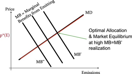
Static setting. The smart tax equals the MD curve. The three downward sloping lines, MB, correspond to the marginal benefit of emissions (the margainal cost of abaement) under different cost shocks. The green arrow identifies the optimal allocation under the high marginal benefits. Under a smart tax (or a smart cap), this point is the market equilibrium where firms equate the marginal benefits from emissions with their private cost of emitting another unit.
Our characterization of the smart cap relies only on the MD curve, not on any information about firms’ technology or shock realizations. We require more information only to pinpoint the particular (first best) equilibrium that arises in the cap and trade market. Using its optimality condition, the representative firm sets marginal benefit from emissions equal to the emissions price
If the marginal benefit is linear, |$\textit {MB}( { {E}}|\theta ) =\theta -f{ {E}}$|, the firm’s optimality condition is13
The conversion function |$q(p)$| depends only on the certificate price; but the equilibrium price, and thus the equilibrium value of the conversion function, depends on the realization of the technology shock. The equilibrium cap is directly proportional to the net benefit |$\theta -a$| of the first unit of emissions, and inversely proportional to the sum of the slopes of marginal costs and damages.
2.2. Heterogenous Firms and the Representative Firm Model
We chose a representative firm formulation for expository purposes, but this assumption is without loss of generality in our setting. We briefly discuss the heterogeneous agent model because the smart cap, unlike the smart tax, introduces a market that aggregates information. This distinction, which is easily overlooked in the representative agent setting, makes the smart cap the superior policy instrument in a real world setting. Here, we show how the smart cap and trade market allows us to aggregate abatement and certificate demand of many firms receiving idiosyncratic (private) shocks, into the decision of a representative firm. Each firm, like the representative firm, operates under the socially optimal price signal. The aggregation result follows immediately from integrating the socially optimal emissions supply into the cap and trade market. Then, the market takes care of optimally decentralizing the abatement decisions; the regulator does not need to know an individual firm’s technology realization. This section formalizes this simple point.
Cap and trade systems, including the smart cap, operate with a market where each firm can buy and sell certificates; these markets are widely established. Here, the market forces lead to a market equilibrium and the market price reflects the marginal abatement cost (of aggregate emissions). Our smart cap is constructed in a way that this market price will equal the social cost of the emissions externality. Crucially, firms’ trades settle their demand for emissions certificates, while the smart cap endogenously regulates the certificate supply to ensure the socially optimal price of emissions. In contrast, under a smart tax, some government entity akin a Walrasian auctioneer would have to solicit demand schedules in order to then fix the correct prices.
We assume a continuum of firms |$i\in I\subset {\mathbb {R}}$| and denote the state of the world by |$s\in S$|, where the set S can be discrete or continuous. For each state of the word, the random variable |$\theta _i:S\rightarrow \Theta$| defines the idiosyncratic shock to firm i, implying firm i’s marginal benefits from emissions |$\textit {MB}_i({ {E}}_i|\theta _i(s))$|. Each firm’s emissions depend on its own technology realization, known only to this firm. As with the representative firm, we assume marginal benefits of emissions to be positive and strictly decreasing in |${ {E}}_i$| for any |$\theta _i(s)$|. Given that the regulator has created a market for emissions, all firms face a common emissions price |$p^E$|. Given any |$\theta _i(s)$|, firm i’s optimal emissions level satisfies
the marginal benefit function is invertible because it is strictly decreasing. The aggregate emissions level is
Because each |$\textit {MB}_i^{-1}( p^E |\theta _i(s) )$| is strictly decreasing in |$p^E$| for all i, given s, so is |$MB^{-1}( p^E |s)$|. Inverting the relation |${ {E}}(\theta _i(s),p^E)= MB^{-1}( p^E |s)$| for a given state of the world s defines the marginal benefits from emissions of the corresponding representative firm |$\textit {MB}({ {E}}|s)$|.14 Following the original description of the smart cap for a representative firm, the smart cap steers the price along the MD curve. As equation (5) demonstrates, each firm optimizes their profits knowing their own technology realization. The firm therefore equates marginal costs from emissions with the social MDs.
For example, in the case of linear-quadratic benefits each firm sets
The aggregate demand for emissions becomes |${ {E}}(\theta (s),p^E)=\int _i {(\theta _i(s)-p^E)}/{f_i} \ di .$| Defining |$f\equiv \left( \int _i {1}/{f_i} \ di \right)^{-1}$| and |$\hat{\theta }(s)\equiv f \int _i {\theta _i(s)}/{f_i} \ di$|, we find a linear-quadratic representative firm with marginal benefits |$\textit {MB}( { {E}}|\hat{\theta })=\hat{\theta }-f{ {E}}$|, where we suppressed the underlying state of the world s, consistent with our earlier notation.
2.3. Dynamic Insights
Climate change is a dynamic problem. As emissions accumulate in the atmosphere, MDs likely increase. Here, optimal policy depends on the shadow cost of the pollution stock, called the SCC in the climate setting. Today’s innovation affects future abatement costs, altering future emissions levels, thus affecting future pollution stocks. Thus, today’s technology shock affects the present discounted stream of future MDs (the SCC). Therefore, we write the SCC as |$\textit {SCC}(E|\theta )$|, a function of emissions, conditional on the shock realization. We assume that |$\textit {SCC}(E|\theta )$| is positive and continuously differentiable in both arguments. Here, to explain the basic insight as simply as possible, we take the function |$\textit {SCC}(E|\theta )$| as exogenous; Section 3 derives this function from primitives.
Social optimality is now characterized by the first order condition
We denote the optimal emissions level satisfying equation (6) as |$E^{*}(\theta )$|, and its inverse as |${E^{*}}^{-1}(E)$|.15 We denote the smart tax by |${ {SCC^{*}\!}}(E)$|. This smart tax, by conditioning on aggregate emissions, satisfies the social optimality condition (6) for all realizations of |$\theta$|. The smart tax is a function of emissions but not the shock:
Under the smart tax the market equilibrium satisfies |${ {MB}}(E|\theta )= { {SCC^{*}\!}}(E)$| by construction, delivering the first best emissions level at the optimal carbon price. Once we have the smart tax, we can decentralize the equilibrium using a smart cap, as in Section 2.1. The smart cap uses the market to provide the price signal required for individual firms to set emissions optimally.
Proposition 1 shows that the optimal price-emissions response no longer traces out MDs: the smart tax |$\textit {SCC}^{*}$| is generally not identical to the |$\textit {SCC}$|. It is easiest to discuss the price-emissions response using the smart tax in emissions space |$(E,p^E)$|, instead of the smart cap in certificate space |$(q,p)$|. We note that Figure 1 simultaneously represents the smart cap translated into |$(E,p^E)$|-space. Proposition 1 evaluates the slope of the smart tax and the slope of the SCC at |$E^{*}(\theta )$| for a given shock realization |$\theta$|. The cases depend on the relative responsiveness of marginal benefits |$\textit {MB}(E|\theta )$| versus MDs (|$\textit {SCC}$|) to a realization of the shock. We introduce the notation |${ {SCC}}_\theta$| for |${\partial \textit {SCC}({ {E}}|\theta )}/{\partial \theta }$|.
|$0 < { {SCC}}_\theta < { {MB}}_\theta \Rightarrow { {SCC^{*}\!}}_E > { {SCC}}_E.$|
|${ {SCC}}_\theta ={ {MB}}_\theta \Rightarrow { {SCC^{*}\!}}_E = + \infty .$|
|${ {MB}}_\theta < { {SCC}}_\theta \Rightarrow { {SCC^{*}\!}}_E < 0 \,\, (< { {SCC}}_E).$|
|${SCC}_\theta =0 \Rightarrow { {SCC^{*}\!}}_E ={ {SCC}}_E \,\, ({as \, in \, the \, static\,setting}).$|
|${ {SCC}}_\theta < 0 \Rightarrow { {SCC^{*}\!}}_E < { {SCC}}_E \,\, ({ { {SCC^{*}\!}}_E\, can\, be\, negative}) .$|
In case (iv), the |$\textit {SCC}$| is unresponsive to the technology shock, |${ {SCC}}_\theta =0$|. Only then does the optimal policy steer carbon prices along the MD curve, as in the static setting of Section 2.1, where no chain of dynamic events correlates future damages from today’s emissions with today’s technological progress. In all other cases, the optimal price-emissions responsiveness differs from the slope of MDs (|$\textit {SCC}$|).
Figure 2 illustrates Proposition 1(i). The solid curves labeled |$\textit {MB}$| and |$\textit {MD}$| show the marginal benefits and the social cost from a unit of emissions (here, the SCC), given the expected technology level |$\theta$|. If the realization of |$\theta$| equals its expected value, the intersection of these curves identifies the optimal emissions level. The dashed curves correspond to a lower realization of |$\theta$|, implying cheaper than expected abatement, for example, due to an unexpected innovation in green technology. The figure assumes that the shock to current abatement costs also reduces future abatement costs, thereby reducing future emissions, Given convex damages, the lower future emissions reduce the future MDs associated with today’s emissions, causing the SCC to shift down to the dashed curve.
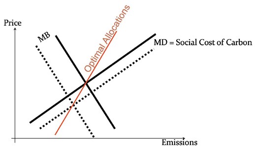
Dynamic setting. The optimal carbon tax (smart tax, red) as a function of the emissions level. The MD curve depicts the marginal damages from emissions, here the social cost of carbon. Black solid lines depict the expected MD and MB curves. Dashed lines depict the case of a better than expected technological innovation. As in the static setting, the innovation shifts down the marginal benefits from emissions curve (abatement cost). In contrast to the static setting, the technological innovation now also shifts down the MD curve: better technology in the future reduces future emissions and, thereby, reduces the MD caused by today’s emissions. The smart tax no longer coincides with (any of) the MD curve.
In Figure 2, the |$\textit {MB}$|-curve responds more strongly to the technology shock than the |$\textit {MD}$|-curve (SCC-curve), corresponding to case i of Proposition 1 (|$0\ \lt { {SCC}}_\theta \ \lt { {MB}}_\theta$|). As a result, the optimal allocation for the depicted low realization of |$\theta$|, shown as the intersection of the dashed lines, lies to the lower left of the expected allocation. Shifting both curves for all possible realizations of the shock, and marking their intersections, results in the set of optimal |$(E,p^E)$| combinations. In the linear quadratic case, all curves—including the set of optimal allocations—are straight lines and we obtain the optimal policy by connecting the two intersections in Figure 2 (one for the expected realization, and one for the actual realization). The corresponding red line is the smart tax. Its slope is positive and larger than the slope of MDs (SCC), illustrating Proposition 1(i). The optimal emissions level is less responsive to a change in the emissions price than the slope of the MD curve would suggest.
Figure 3 represents cases (ii) and (iii) of Proposition 1. If the technological innovation shifts the |$\textit {MD}$| curve and the |$\textit {MB}$| curve by the same amount (|${ {MB}}_\theta ={ {SCC}}_\theta$|), then the smart tax is vertical (left graph). In this case, a standard cap and trade system is optimal regardless of the relative slopes of the |$\textit {MB}$| and the |$\textit {MD}$| curves. If the technological innovation shifts the |$\textit {MD}$| curve more than it shifts the |$\textit {MB}$| curve (|${ {MB}}_\theta \ \lt { {SCC}}_\theta$|), then the slope of the smart tax is negative. In this case, it is optimal to emit more under a lower tax despite the lower abatement costs, because the improved technology makes the climate problem less severe.
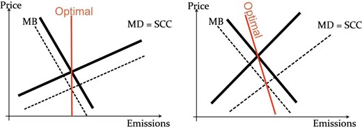
Dynamic setting, analogous to Figure 2. The optimal carbon tax (smart tax, red) as a function of the emissions level. If the MD curves shifts down as much as the MB curve, the smart tax is vertical and a standard cap and trade system is first best (left). If the MD curves shifts more that the MB curve, the smart tax falls with emissions (right). Here, a low emissions price signals sufficiently large falls in future abatement costs that it is optimal to increase current emissions.
We already mentioned that the fourth case in Proposition 1 is analogous to the static case. Here, the |$\textit {SCC}$| curve does not respond to the technological innovation, and it directly gives the smart tax. The fifth case describes the scenario where a shock increases abatement costs but reduces MDs. Here, the slope of the smart tax is smaller than the slope of the |$\textit {MD}$| curve (and possibly negative). Our quantitative analysis in Section 3 identifies case (i) of Proposition 1 and Figure 2 as the most likely (or at least “base”) scenario in the case of climate change. It also gives examples of cases (ii) and (iii). Case (iv) would arise if we neglect the dynamic nature of the climate change problem, or if climate damage are not convex. Our dynamic model in Section 3 does not give rise to case (v).
To translate the results in Proposition 1 from |$(E,p^E)$|-space into the |$(q,p)$|-space for certificates, we replace |$\textit {MD}$| by |${ {SCC^{*}\!}}$| in equation (4) of Section 2.1:
The right side uses the definition of the conversion function’s elasticity w.r.t. the certificate price,
In cases (i) and (iv) of Proposition 1, the shock response of MDs is non-negative but smaller in magnitude than that of the abatement cost curve. Then, the slope of the smart tax is positive, that is, the tax increases in emissions; equivalently, optimal emissions increase with the price of an emissions unit. In these cases, the left side of equivalence (8) shows that the smart cap, and thus emissions, also increase as a function of the certificate price. In case (ii) the shock response of MDs equals that of marginal abatement costs (Figure 3 on the left). Here, where the slope of the smart tax is infinite, the smart cap corresponds to a standard cap, which does not respond to the price.
In case (iii) MDs are more sensitive than abatement costs to the shock, and in case (v) the MD response has the opposite sign of the marginal abatement response. In both cases, the slope of the smart tax is negative. The left side of equivalence (8) shows that the slope of the conversion function |$q(p)$| is generally ambiguous. The right side of the equivalence (8) shows that the smart tax is negatively sloped if either the smart cap has a positive slope and is elastic with respect to the certificate price (|$\epsilon _{q,p}(p)\ \gt 1$|) or if the smart cap has a negative slope (|$\epsilon _{q,p}(p)\ \lt 0$|). The next section shows that the relation between the signs of the slopes of the two functions is unambiguous when the equilibrium is stable.
2.4. Stability
This section analyzes market stability when regulating emissions using a smart tax or smart cap. Here, we assume existence of a well-defined smart tax function or a smart cap’s conversion function; Section 3 shows existence constructively for a particular model.16 We use the standard definition of Walrasian stability: the equilibrium price is locally stable if and only if the excess demand slopes down at the equilibrium price (Mas-Colell, Whinston, and Green 1995). Global stability requires that excess demand is positive whenever the price is below the equilibrium price and negative whenever the price is above the equilibrium price. Our stability analysis restricts attention to the price domains of the smart tax or cap that can support a social optimum under some feasible technology realization |$\theta$|, that is, prices that are part of our construction of the smart tax or cap on the relevant policy domain. In addition to existence and our assumptions at the beginning of Sections 2.1 and 2.3,17 this section also adopts
The inequalities (i) |$\textit {SCC}_E(E|\theta ) \ge 0$| and (ii) |$\textit {SCC}_{\theta }(E|\theta ) \ge 0$| hold with complementary slackness. The interval of possible technology realization |$\theta$| is closed and connected.
Inequality (i) assumes that damages are weakly convex and slightly weakens our assumption in Proposition 1 to allow for a completely flat |$\textit {SCC}$|. In exchange, inequality (ii) focuses our attention on the case of interest where an abatement-cost reducing technology innovation today reduces the SCC by reducing current and future abatement costs. We assume that these weak inequalities hold with complementary slackness: the SCC strictly increases in either the pollution stock or the technology shock, or both. Lemma C.1 in the Online Appendix shows that, as a result, |${ {SCC^{*}\!}}_E\ne 0$| even if the SCC is flat.
The following result maintains our previous assumptions summarized in footnote 17, existence, and Assumption 1. It employs the elasticity of the socially optimal emission response to a change in the emission price |$\epsilon _{E,p^E}$|, which coincides with the implicit emission supply response resulting from a smart tax. A tax regime does not actually introduce a market. When we discuss stability, we assume a hypothetical market implementation of the smart tax where firms submit their demand schedules and the regulator offers emissions allowances according to the smart tax schedule.
The equilibrium under a smart tax is globally stable.
The equilibrium under the smart cap is globally stable if and only if any of the following equivalent statements hold:
The slopes of the smart cap’s conversion function and of the smart tax have the same sign.
The smart tax’s emission supply elasticity to price changes satisfies |$\epsilon _{E,p^E}\ \gt -1$|.
The conversion function’s elasticity to changes in the certificate price satisfies |$\epsilon _{q,p}\ \lt 1$|.
The smart cap is always stable if the smart tax is increasing in emissions, and it is always stable if the smart cap is decreasing in the certificate price.
Under a positively sloped smart tax, the equilibria under both a smart tax and a smart cap are stable. The smart cap’s market equilibrium remains stable if it’s conversion function slopes down. However, if the smart tax is negatively sloped but the smart cap’s conversion function is upward sloping, then the market equilibrium is unstable under a smart cap. This happens if either of the (equivalent) elasticity conditions (b) or (c) are violated. The proof of Proposition 2 also shows the condition in terms of the model fundamentals. This slightly more cumbersome expression shows that convexity of damages and concavity of emission benefits work against instability, but suggests that instability can arise if the SCC is large and responds much more strongly to the technology innovation than marginal abatement costs (|$\textit {SCC}_\theta \ \gt \ \gt \textit {MB}_\theta$|).
2.5. Endogenous Abatement Costs
For the most part we assume that the abatement cost function depends on only emissions and the exogenous shock, |$\theta$|. In reality, firms choose other inputs, for example, abatement capital, that alter their abatement costs. The fact that the smart cap delivers the first best abatement level for every realization of the cost shock means that the regulator has no need for additional policies that target investment or other inputs.18 A two-stage example illustrates this claim.
In the first stage, the representative non-strategic firm chooses investment before observing the cost shock. In the second stage, after observing the shock, the firm chooses the level of pollution. Thus, the second stage reproduces our representative firm model in Section 2.1, apart from the fact that the second stage equilibrium now depends on the first stage choice of capital. This difference is not important; the equilibrium typically depends on many parameters that are exogenous or predetermined at the emissions stage. Here, we make the dependence on capital explicit. Under the smart cap, the firm faces a stochastic future price of emissions. This price arises from the market equilibrium, given a technology realization |$\theta$| and given capital investment k. We denote this emissions price by |$\tilde{p}^E(\theta ;k)$|. The non-strategic firm, under a smart cap, chooses the same capital investment in the first stage as a social planner who has the same information as the firm and incorporates the externality.
The firm’s decision problem is19
At the investment stage, the firm treats the cost shock, |$\theta$|, and the resulting permit price, |$\tilde{p}^E$|, as random variables. The firm incurs investment costs |$c(k)$|. The function |$B(\cdot )$| specifies the benefit of emitting E, given the cost shock |$\theta$| and the level of capital k (Footnote 9). By equation (9), the firm’s second-stage optimality condition is |$B_E(E,k|\theta )=\tilde{p}^E(\theta ;k)$|. We denote the emissions solution by |$\tilde{E}(k|\theta )$|, which is again conditional on k and |$\theta$|.
The planner’s problem is
The planner’s second-stage optimality condition is |$B_E(E,k|\theta ) = D^{\prime }(E)$| for all k and |$\theta$|. Section 2.1 shows that the smart cap induces the optimal level of emissions for every realization of |$\theta$| (given k). The argument in that section therefore establishes that the second-stage price under a smart cap satisfies |$\tilde{p}^E(\theta ;k)=D^{\prime }(E)$| for all k and |$\theta$|. Consequently, the individual firm and the social planner chose the same equilibrium level of pollution, |$\tilde{E}(k|\theta )$|, given k and |$\theta$|. Therefore, the firm and planner have the same first order condition for investment, |$c^{\prime }(k) = {\mathbb {E}}_{\theta } B_k(\tilde{E}(k|\theta ),k|\theta )$|. A firm’s investment into green capital under a smart cap coincides with the socially optimal investment.
3. The Dynamic Model
This section uses a dynamic version of Weitzman’s (1974) static linear-quadratic model. The smart tax implements the full-information (first best) level of emissions as a unique stable competitive equilibrium. The full-information |$\textit {SCC}$| increases with emissions, but the smart tax might either increase or decrease in emissions. We use the smart tax to construct the conversion function for the smart cap, as in Section 2.1. The smart tax provides an extremely simple way of expressing the welfare ranking of the standard tax and quota, one that exactly parallels Weitzman’s ranking for the static model. We also examine certificate trading across periods and quantify the smart cap and smart tax.
3.1. Model and Analytic Results
We measure the pollution stock |$S_{t}$| at the beginning of period t by its deviation from the zero-cost level (e.g. the pre-industrial level of GHG). The stock of pollution at the end of the period is
where the parameter |$\delta$|, |$0\ \lt \delta \le 1$|, measures the pollutant’s persistence.
At the beginning of period t, the policy maker and firms know the value of the random variable |$\theta _{t-1}$|. In our primary example, this variable characterizes—apart from a deterministic trend |$h_t$|—the innovated technology in the economy; a negative shock corresponds to higher than expected progress. Firms, but not the policy maker, then observe the innovation |$\varepsilon _{t}\sim iid\left( 0,\sigma ^{2}\right)$|.20 Firms solve a succession of static problems. In each period, the market for certificates aggregates heterogeneous firms’ individual shocks. Therefore, we can apply the procedure developed Section 2.2 to replace the heterogeneous agent model with a representative agent. Thus, we have the equation of motion
with shock (or technology) persistence |$0\ \lt \rho \le 1$|.21 The realization of |$\varepsilon _{t}$| alters the marginal benefit of emissions, via a change in technology affecting emissions intensity, or a change in economic activity affecting emissions demand.
Only a fraction, |$0\ \lt \alpha \le 1$|, of this innovation is adopted in the current period, so firms in period t operate with technology level
We can interpret |$\alpha$| as a share of firms adopting the new technology in the current period, as in the literature on technology diffusion (Rogers 1995). More generally, a higher |$\alpha$| represents a quicker response of firms to the shock.22
The benefits from emissions (or abatement costs) are quadratic; the linear contribution depends on the technology level |$h_{t}+\hat{\theta }$|, where |$h_t$| denotes the deterministic trend:
Marginal benefits of emissions are then |${\partial B}/{\partial E}=h_{t}+\hat{\theta }_{t}-fE_t$|, with |$f\ \gt 0$|. Hereafter, we assume that the marginal benefits at zero emissions, |$h_{t}+\hat{\theta }_{t}$|, and the full-information (first best) level of emissions are both positive with probability one. Flow damages are quadratic in the pollution stock
with |$b\ \gt 0$|. The policy maker with discount factor |$0\ \lt \beta \ \lt 1$| maximizes
The policy maker is aware that future optimal emissions policies depend on the future realizations of the state variables.23
In the static model (Section 2), the smart tax or cap adjusts automatically to support the optimal level of emissions. There, the regulator learns the state of the world, |$\theta$|, by observing the market outcome, but has no need for more information. In the dynamic setting, the regulator begins the period knowing |$\theta _{t-1}$|. The automatic adjustment in the smart tax or cap again supports the first best emissions level, and enables the regulator to learn the current innovation, |$\varepsilon _t$|. The regulator uses that information and equation (10) to update |$\theta _t$|.
We now explain the derivation of the smart tax. In Section 2.3, we took the function |$\textit {SCC}(E|\theta )$| as exogenous. Here, we recognize that the social cost of carbon, |$\textit {SCC}(S_t, \theta _{t-1}, \varepsilon _t)$| is an endogenous function. We therefore first solve the full information optimum to obtain both |$\textit {SCC}(S_t, \theta _{t-1}, \varepsilon _t)$| and the full information emissions policy, which is also a function of |$(S_t, \theta _{t-1}, \varepsilon _t)$|. We then obtain the smart tax much as in Section 2.3. By construction, the non-strategic representative firm facing this smart tax emits at the socially optimal level. Online Appendix D provides details.
- The smart tax is(11)$$\begin{eqnarray} \textit {SCC}_{t}^{\ast }=A_{0}S_{t}+A_{1}\theta _{t-1}+\gamma E_{t}+a_{t}. \end{eqnarray}$$
- The smart tax’s emissions’ slope, |$\gamma$|, can take either sign. There exists |$\alpha ^{*}\in (0,\beta )$| such that for |$\alpha \ \gt \alpha ^{*}$|and for |$\alpha \ \lt \alpha ^{*}$|(12)$$\begin{eqnarray} \gamma = \frac{\partial \textit {SCC}_{t}^{\ast }}{\partial E_{t}}\ \gt \frac{\partial \textit {SCC}_{t}}{\partial E_{t}} \ \gt 0 \end{eqnarray}$$For |$\alpha =\alpha ^{*}$|, the slope of the smart tax is infinite, and a conventional cap and trade achieves the first best emissions allocation. As |$\alpha$| passes through |$\alpha ^{\ast }$| (from below), the slope of the smart tax switches from |$-\infty$| to |$+\infty$|, and for |$\alpha \ \gt \alpha ^{\ast }$| the slope of the smart tax decreases continuously in |$\alpha$|.(13)$$\begin{eqnarray} \gamma = \frac{\partial \textit {SCC}_{t}^{\ast }}{\partial E_{t}}\ \lt 0 \mbox{ and } \frac{\partial \textit {SCC}_{t}}{\partial E_{t}} \ \gt 0 . \end{eqnarray}$$
The smart tax supports the optimal level of emissions as a globally stable competitive equilibrium for all |$\alpha \in (0,1]$|, that is, for both positive and negative |$\gamma$|.
Proposition 3 shows that our dynamic model can produce cases (i)–(iii) of Proposition 1.24 The smart tax provides a stepping stone to derive the smart cap, and it shows the role of the speed of technology adoption. It also leads to a simple criterion for welfare-ranking a standard tax and cap, and relating that criterion to Weitzman’s (1974) result for a flow pollutant (see Proposition 5).
For quick technology diffusion, |$\alpha \approx 1$|, a positive shock |$\varepsilon _t$| causes a larger increase in the marginal benefit of emissions than in the SCC (|$\textit {MB}_{\varepsilon }\ \gt \textit {SCC}_{\varepsilon }$|) and the smart tax is steeper than the |$\textit {SCC}$| (case (i) in Proposition 1). In this case, for example, lower than expected technological progress increases the optimal emissions, partly offsetting firms’ higher than expected abatement costs. For |$\alpha$| small, a shock has little effect on the present period’s marginal benefit of emissions, but has a non-negligible effect on the |$\textit {SCC}$|. In this case, the smart tax has a negative slope (case (iii) in Proposition 1). Here, lower than expected technological progress reduces the optimal emissions level because it increases future climate damages without substantially affecting firms’ emissions costs in the current compliance period. Finally, if |$\alpha =\alpha ^{*}$|, the shock equally affects marginal benefits and damages from emissions, and a conventional cap and trade-system achieves the first best emissions allocation (case (ii) in Proposition 1). Here, the shock realization’s impact on firms’ abatement costs and the SCC balance each other in a way that preserves a fixed optimal emissions level.
The proposition also shows that a negatively sloped smart tax requires |$\alpha \ \lt 1$|; here the technological innovation is observed but not fully implemented in the current period. Under such slow diffusion, the long-term impact of the new information determining the SCC dominates the short-term impact determining firms’ abatement costs. Regardless of the value of |$\alpha$|, the smart tax implements the social optimum as a stable competitive equilibrium.
We now consider the smart cap. To simplify notation, we define |$\hat{A}_{t}\equiv A_{0}S_{t}+A_{1}\theta _{t-1}+a_{t}$|, which collects all of the time-dependent variables in the formula for the smart tax apart from the current emissions level |$E_t$|. With this definition, the smart tax is |$\textit {SCC}_{t}^{\ast }=\hat{A}_{t}+\gamma E_{t}$|. We follow the same logic as in Section 2.1. The firm’s price of a unit of emissions is |$p^{E}_t={p_t}/{q_{t}\left( p_t\right) }$|. We construct the smart cap so that it implements the optimal level of emissions, for example, we set |${p_t}/{q_{t}\left( p_t\right) }=\hat{A}_{t}+\gamma E_t$|. The subscript on |$q_{t}$| serves as a reminder that the conversion function depends on time via the function |$\hat{A}_{t}$|.
Proposition 4 gives the precise form of the optimal smart cap for the linear-quadratic dynamic model. It shows, consistent with Proposition 2(iii), that the slopes of the smart tax and cap have the same sign. Using Proposition 3, we know that a slower speed of technology adoption increases the parameter set for which these slopes are negative.
Figures 4–6 in our quantitative Section 3.3 illustrate the smart tax and the corresponding smart cap. Consistent with Proposition 2 for the general case, the smart cap in our dynamic model is stable and increases with the certificate price when the smart tax increases (|$\gamma \ \gt 0$|). Here, the smart cap expands when the certificate price increases and it contracts when the certificate price falls. For |$\gamma \ \lt 0$|, where the smart tax falls with emissions, the smart cap shrinks as the certificate price rises.25
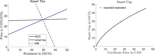
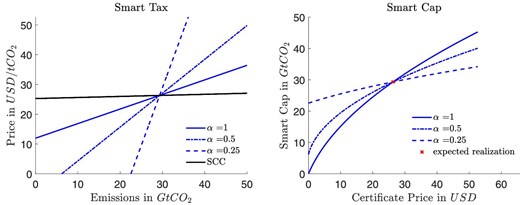
Calibrated smart tax and cap. Left: SCC and marginal benefits of emissions (MB) under the expected technology realization as well as smart tax (independent of technology realization). Right: Smart Cap, which is the conversion function times expected emissions.
Variations of speed of technology adoption. Immediate full adoption (|$\alpha =1$|), half of firms adopt during a 5-year compliance period (|$\alpha =.5$|), one quarter of firms adopts during a 5-year committeemen period (|$\alpha =.25$|). Left: Smart tax. Depicted SCC assumes expected technology realization. Right: Smart Cap.
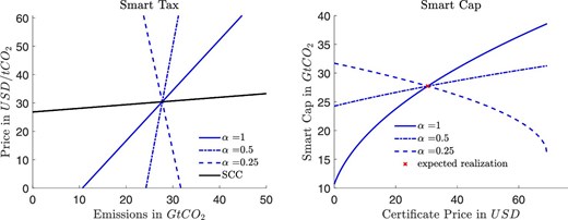
Concerned scenario. Smart tax (left) and smart cap (right) assuming a higher damage convexity. The different curves correspond to immediate full adoption (|$\alpha =1$|), half of firms adopting (|$\alpha =.5$|), and one quarter of firms adopting during a 5-year compliance period (|$\alpha =.25$|).
The market response to either the smart tax or the smart cap enables the regulator to recover one piece of hidden information. Optimal policy depends on the persistence |$\rho$| and the speed at which firms respond to the shock, measured by |$\alpha$|. We can interpret the shock as being related either to technology or to the business cycle. A technology shock tends to be genuinely asymmetric information. Firms’ response to the policy reveals the hidden technology shock. The macro shock is unknown when the regulator announces the smart tax or smart cap, but observed by both firms and the regulator during the compliance period. Therefore, the policy can be conditioned on the macro shock. If the macro shock is i.i.d., we do not need to modify the model presented above. More plausibly, if expectations of the macro shock depend on information such as current and lagged macro conditions, those variables become part of the information set. The full information |$\textit {SCC}$| and both the smart tax and the smart cap then depend on those variables, but the structure of the policy does not change.
A famous result, due to Weitzman (1974), states that in the linear-quadratic model with additive shocks and a flow pollutant, the standard tax welfare-dominates the standard quota if and only if the slope of MDs is less than the slope of marginal abatement costs (equal to the slope of marginal benefit of emissions). The literature cited in footnote 8 studies the more complicated welfare comparison between the standard tax and quota for a stock pollutant. The smart tax provides a novel and intuitive link between the models with flow and stock pollutants. Section 2.1 notes that the MD function coincides with the smart tax for a flow pollutant. Thus, for a flow pollutant, we can restate Weitzman’s result as “For a flow pollutant, taxes welfare-dominate quotas if and only if the slope of the smart tax is less than the slope of marginal abatement costs”. In this formulation, Weitzman’s classical result extends to the more policy-relevant setting of stock pollutants:
With stock pollutants, (standard) taxes welfare-dominate (standard) quotas if and only if the slope of the smart tax, |$\gamma$|, is less than the slope of the marginal abatement cost, f.
3.2. Inter-Period Trading and Optimality
At least eight cap and trade programs, including California’s Low emissions Vehicle Program, the EPA’s SO2 and NOX programs, and the EU’s Emissions Trading Scheme, allow intertemporal banking of permits Holland and Moore (2013). Intertermporal trading can smooth carbon price fluctuations triggered by shocks, potentially increasing welfare. A smart cap does not require intertemporal trading, because emissions respond to shocks optimally by construction. Intertemporal trading may nevertheless be relevant if the compliance phase is long or if the institutional framework does not permit conditioning the smart cap on macroeconomic indices.
As in our base setting, a conversion function |$q_t(p_t)$| characterizes the price–quantity relation within a period. We now assume that the regulator allows interperiod trading within a compliance phase lasting T periods. Firms can trade certificates across the T periods; the certificate cap, Q, applies to the entire compliance phase. Later compliance phases might have a different number of periods, but we assume that policy is set optimally in the future; the horizon is infinite; and the certificates of the current compliance phase cannot be used in later compliance phases. Firms in previous sections do not have to make intertemporal decisions. Keeping with this setting, we assume the existence of a risk neutral arbitrageur that makes firms indifferent about the timing of certificate purchases. Our setting allows for two interpretations: firstly, it examines the implications of introducing multiple trading periods within a 1-year compliance phase; secondly, it explores a scenario analogous to banking and borrowing, where firms are permitted to utilize certificates across different years—for instance, with a period length of 1 year and a compliance phase spanning 5 years.
To avoid the need for double-subscripts, we consider the case of the first T-period compliance phase, with the initial period set at |$t=1$|. The smart cap’s conversion function in period t, |$q_{t}(p_t)$|, determines the exchange ratio |$q_{t}$| between certificates and CO|$_2$| emitted in period t. For |$E_t$| emissions in period t, the representative firm has to deliver |${E_t}/{q_t}$| certificates at the end of the compliance phase. Market clearing requires |$\sum _{t=1}^T {E_t}/{q_t} = Q$|, where Q is the total number of certificates for this compliance phase. Focusing on the fundamental issues of inter-period trading, we assume that innovations are immediately adopted: |$\alpha =1 \Rightarrow \hat{\theta }_{t}=\theta _{t}$|.
There exists a sequence of conversion functions |$q_t^{p_1,\ldots ,p_{t-1}}(p_t)$|, |$t \in \lbrace 1,\ldots ,T\rbrace$|, and an allocation of certificates |$Q(p_1,\ldots ,p_{T-1})$| supporting the optimal emissions trajectory as a decentralized intertemporal equilibrium.
The aggregate number of certificates for this compliance phase depends on the sequence of certificate prices within that phase. If the aggregate number Q was fixed, the certificates remaining at the beginning of period T would be stochastic. However, a given conversion function |$q_T$| achieves the first best allocation only for a specific number of certificates. Therefore, the aggregate number of certificates has to depend on the earlier prices to guarantee that the number of certificates remaining in period T, together with the conversion function in that period, support the optimal emissions level.
Under banking and borrowing—in both a standard and a smart cap—intertemporal arbitrage implies that the price of certificates has to rise at the rate of interest. An emissions price growing at the rate of interest is generally not optimal, which is an issue for standard emissions trading schemes. Proposition 6’s period-dependence of the conversion function, that is, the exchange ratio between emissions and certificates, decouples the price increase of emissions from the intertemporal arbitrage condition to achieve first best.26
Proposition 6 conditions the conversion functions on the certificate price in earlier periods. Such conditioning allows the mechanism to incorporate the carbon stock fluctuations resulting from the sequence of technology shocks over the course of a compliance phase. Over a fairly short compliance phase, for example, a decade, the stock of carbon is likely to vary much less than the technology variable. Then, it seems reasonable to neglect a conditioning of the conversion functions on the earlier period’s price realizations.
3.3. Quantification
We use our results to study global climate change. As the introduction notes, many countries are either planning to use or currently using taxes or cap and trade systems to reduce their CO|$_2$| emissions. We quantify the smart tax and cap when there is global cooperation.
Output, Abatement, and Emissions.
Global annual world output in 2020 is 130 trillion USD using purchasing power parity weights (IMF 2020). We use Nordhaus and Sztorc’s (2013) DICE model to estimate the 2020 marginal abatement cost slope as |$f = 2.5\times 10^{-9}\, {{\rm {USD}}}/{{t {\rm {CO}}_2}^2}$|. Much of our analysis depends only on the slopes of the marginal abatement cost and MD curves. The absolute levels of the SCC also depends on |$h = 101\, { {\rm {USD}}}/{{t {\rm {CO}}_2}}$|, the intercept of marginal abatement costs. We assume that this intercept falls exogenously by 1% per year.27 This calibration implies a business as usual emissions level of |$E^{ {\rm {BAU}}}=40{ {Gt {\rm {CO}}_2}}$| per year, implying that we have been abating a few percent of business as usual emissions in 2020.
Technology Diffusion.
We obtain an estimate (or guesstimate) of the technology diffusion parameter |$\alpha$| by regressing US CO|$_2$| emissions in 1995–2010 against (stocks and flows of) green patents. We assume 5-year compliance periods and |$\rho =1$|, that is, no decay of innovations (patents).28 We restrict attention to “major” green patents, those registered in all three major patent offices, United States, Europe, and Japan. We summarize details in the Online Appendix F.29 Our preferred estimate lies slightly above |$\alpha \approx 0.25$|; about one quarter of the long-run impact of the innovation shocks occur within the current compliance phase. Other relevant innovations, which are not being patented, might be adopted faster leading to a somewhat higher overall adoption share |$\alpha$|. We present results for |$\alpha \in \lbrace 0.25,0.5,1\rbrace$|.
Climate.
We use the model of transient climate response to cumulative emissions (TCRE) to calibrate climate dynamics. Recent climate modeling shows that average global atmospheric temperature can be well-approximated as a linear function of cumulative historic emissions. The consensus report IPCC (2021) states that the proportionality factor between cumulative emissions and temperature, TCRE, is likely in the range between |$1^\circ {\rm C}$| and |$2.3^\circ {\rm C}$| for each 1000 GtC (|$10^{12}$| tons of carbon). We use the reports best estimate of |$1.65*10^{-15}{^\circ {\rm C}}/{GtC}$|.30 Online Appendix G illustrates the corresponding temperature response to emissions and compares it with Nordhaus’s (2017) DICE model and a complex scientific climate model. Our state variable, |$S_t$|, is cumulative historic emissions, which are proportional to temperature; the persistence factor is therefore |$\delta =1$|.
We briefly comment on the intuition of the TCRE model. In the actual climate system, most CO|$_2$| emissions are eventually removed from the atmosphere, but each emissions unit has a cumulative impact on temperature over time through its greenhouse effect. Scientific models of climate change find that the removal of carbon from the atmosphere and the delayed warming response to an increase in carbon concentrations approximately cancel each other, making cumulative historic emissions a good proxy for temperature.
Damages.
DICE assumes no damages at the pre-industrial temperature level and global damages of approximately 1% of world output at a 2|$^\circ {\rm C}$| warming (Nordhaus and Sztorc 2013). Our baseline calibration of the damage function uses this assumptions, producing |$b_{base}=1.3*10^{-13}\, { {\rm {USD}}}/{{t {\rm {CO}}_2^2}}$|. We also introduce a “concerned” scenario that assumes today’s damage from global warming is zero, but a |$3^{\circ }$|C warming causes a loss of 5% of world output. This scenario implies a more convex damage function with |$b_{\textit {concerned}}=6.6*10^{-13}\, { {\rm {USD}}}/{{t {\rm {CO}}_2}^2}$|. We can also interpret this scenario as reflecting concern about tipping points.
Expected Optimal SCC.
We test our calibration by calculating the implied optimal carbon tax under the expected technology realization. At the optimal emissions allocation, the smart tax equals the SCC by construction. For an annual rate of pure time preference (rptp) of |$1.5\%$| (|$\beta =0.985$|) we obtain an optimal carbon tax of |$26{\rm \ USD}/{t {\rm {CO}}_2}$|. This tax is a little higher than in DICE, which has recently been discovered to exaggerate the temperature delay in warming (a feature we avoid by using the TCRE model). Reducing the rptp to |$0.5\%$| (|$\beta =0.995$|), the median response of Drupp et al.’s (2018) expert survey, approximately doubles this tax (|$55{\ \rm USD}/{t {\rm {CO}}_2}$|). These values suggest that the model calibration is reasonable. The corresponding optimal emissions levels are |$E^{\textit {opt}}=29{ {Gt {\rm {CO}}_2}}$| for |$\beta =0.985$|, and |$E^{\textit {opt}}=18{ {Gt {\rm {CO}}_2}}$| for |$\beta =0.995$|. Under the |$1.5\%$| rptp, the concerned scenario using the more convex damage function increases the tax only mildly to |$30{\rm \ USD}/{t {\rm {CO}}_2}$|.31
Results Base Calibration
Figure 4 presents the smart tax and cap assuming a 5-year compliance period and immediate adoption of the new innovation (|$\alpha =1$|). The left panel graphs the smart tax as well as the SCC and the marginal benefits from emissions under the expected technology realization. By construction, all the lines intersect at the expected price and emissions levels. For other realizations of technology, the equilibrium moves along the smart tax. We observe that (i) the smart tax is substantially steeper than the SCC curve and (ii) the (absolute of the) MB-curve’s slope is greater than the slope of the smart tax. Thus, by Proposition 5, if forced to choose between either a standard tax or a standard cap, then taxes are preferred over quantities in this baseline scenario with |$\alpha =1$|.
The smart cap shown on the right of Figure 4 eliminates the welfare loss of a tax. To make it easy to compare the smart tax and the smart cap, we depict the overall (global) cap in |$Gt {\rm {CO}}_2$|. We set the number of certificates, Q, equal to the optimal emissions level under the expected technology realization. With this choice, the certificate price under the expected technology realization coincides with the smart tax of |$26{\rm \ USD}/{t {\rm {CO}}_2}$|. Greener than expected technological progress, causing a downward shift in the demand for emissions (the MB curve), leads to a lower certificate price and a contraction of the smart cap. Similarly, less green technological progress increases the certificate price and expands the smart cap. The conversion function’s graph is identical to that of the smart cap once we change the scale on the vertical axis from aggregate emissions to the emissions level per certificate.
Figure 5 varies the speed of firms’ technology adoption, with the solid graphs replicating those of Figure 4, where |$\alpha = 1$|. The dashed graph uses our preferred estimate |$\alpha \approx 0.25$|, where only one quarter of firms adopt the new technology innovations within the 5-year compliance period. The reduced speed of adoption substantially increases the slope of the smart tax and flattens the slope of the smart cap, which graphs emissions over price rather than price over emissions.We note that the slope of the dashed smart tax exceeds that of the MB-curve (depicted in Figure 4); by Proposition 5, if forced to choose between standard instruments, quantities dominate taxes for |$\alpha =0.25$|. The dashed–dotted line assumes that half of the firms adopt the new innovation during the 5-year compliance period (|$\alpha =0.5$|). This value represents that less fundamental non-patented innovations might also be adopted more quickly, increasing |$\alpha$|. For |$\alpha =0.5$|, the smart tax and the MB-curve have almost the same slope; here, the welfare difference between a tax and a standard cap is close to zero.
Concerned Scenario.
Figure 6 presents the results for the concerned scenario, where damages are more convex (initially lower and then higher).The smart tax and the SCC under the expected technology realization are higher than in the baseline. Both increase faster for lower than expected technological progress; the resulting higher future emissions increase damages more strongly with more convex damages. Similarly, higher than expected green progress reduces the equilibrium prices more strongly; here, a reduction in the future CO|$_2$| stock implies a stronger reduction of future damages than in the baseline. The smart cap, a function of the certificate price, shows the same qualitative features as a function of the certificate price. Reducing the speed of technology adoption, |$\alpha$|, rotates the smart tax graph counter-clockwise (making it steeper) and the smart cap graph clockwise (making it less steep). Reducing the speed of adoption makes the shock relatively less relevant for firms’ current abatement costs as compared to its sustained impact on long-term damages. For |$\alpha \lessapprox 0.4$|, the smart tax and cap have negative slopes (see as well right graph in Figure 7).
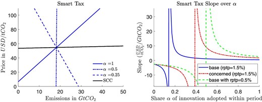
Left: Smart tax under the baseline calibration but with a reduced rate of pure time preference (0.5% instead of 1.5%). The share |$\alpha$| of immediate adopters varies in three discrete steps from one to one quarter. Right: Slope of the smart tax. The share |$\alpha$| of immediate technology adopters varies continuously along the horizontal axis and the three curves correspond to the different scenarios.
In particular, our estimate |$\alpha \approx 0.25$| implies a decreasing smart tax and cap. Here, a higher than expected green technological progress not only lowers the cost of abatement, but also reduces long-term damages sufficiently that it is optimal to respond with both a price reduction and an emissions increase (moving down on the smart tax graph and up on the smart cap graph). The planner knows that most of the improved technology will be adopted in the next period, lowering future emissions and the MD associated with current emissions. Similarly, less green progress increases the emissions price and, given the damage convexity, urges us to cut more emissions.
Given the novelty of this finding, it is worth discussing a variation of the intuition. Lower than expected green progress is bad news for both firms and the environment. In the baseline scenario (or, here, for |$\alpha \ge 0.4$|), the optimal policy uses the environment to smooth shocks to the firms; if abatement turns out to be very expensive, then we allow firms to emit more. However, if damages are sufficiently convex and |$\alpha$| is low, the future environmental damage implied by the lack of green progress is too costly to tolerate such smoothing at the expense of the environment. Instead of using costs to the environment as a substitute for costs to the firms, the policy maker now treats them as complements. Under bad news we increase the unit price and cut emissions. Conversely, under good news, we lower the price and permit firms to emit more.
Reduction of Time Preference.
The left graph in Figure 7 reduces the rptp from an annual |$1.5\%$| to |$0.5\%$| in the base scenario. The implications are qualitatively similar to those observed in the previous variation with more convex damages. Here, the policy maker pays more attention to future damages. As a result, the SCC under the expected realization increases substantially and the smart tax rotates counter-clockwise for any speed of technology adoption. An adoption share of |$\alpha =0.5$| during the 5-year compliance period makes the smart tax vertical and the smart cap horizontal (not shown). Under these assumptions, the smart cap corresponds to the classical cap; the ordinary cap and trade system reaches first best.
Slope over Adoption Share.
The right panel of Figure 7 plots the slopes of the smart tax over the “speed of adoption”, that is, the share |$\alpha$| of firms that adopt the new innovation within the 5-year compliance period. Starting from the right, we observe that the smart tax is most sensitive to emissions under the reduced discount rate and more sensitive in the concerned scenario than in the baseline. This difference in slope (sensitivity) increases as we reduce the share |$\alpha$|. The vertical lines identify the values of |$\alpha$| at which the slope of the smart cap flips sign: |$\alpha \approx 0.5$| for the rptp of |$0.5\%$| (green dashed), |$\alpha$| just below |$0.4\%$| for the concerned scenario (red dash-dotted), and in the base scenario the adoption share within the compliance period would have to fall all the way to |$\alpha =0.14$| (half or our preferred estimate) to turn a standard cap first best.
4. Practical Implementation of a Smart Cap
This section discusses the practical implementation of the smart cap and some easily implemented compromises to improve efficiency in pre-existing cap and trade systems. In the real world, (i) business cycles have a major impact on emissions and certificate prices, (ii) information is revealed continuously over the course of a compliance phase and certificates are traded continuously, and (iii) political institutions tend to favor simplicity and minimal change. While the smart cap can help with point (i), we repeat that it is better to deal with this issue by explicitly conditioning the (smart or standard) cap on GDP or alternative business cycle indicators. Thus, this section is mostly concerned with points (ii) and (iii). That said, much of this discussion also applies to cost shocks generated by business cycles or other sources of price shocks.
Regarding period length, Section 3.2 explains how a sequence of announced conversion functions can achieve or improve efficiency when shocks and trading occur repeatedly during a compliance period. For example, we can choose annual (or monthly) compliance periods, or we can choose annual (or monthly) conversion functions while using a 5-year compliance period, where firms use and trade the same certificates over the 5-year period. Proposition 6 would motivate a dense sequence of conversion functions that respond directly to preceding price realizations. Such conditioning enables the smart cap to respond to the small fluctuations of the CO|$_2$| stock during a compliance period, but these are of minor quantitative relevance during a 5-year commitment period. Therefore, we simply recommend an annual conversion function using a weighted average of carbon prices over the course of the year. Certificates will be traded throughout the year, and beyond. 32 The annual conversion functions can be announced for a 5-year compliance period, changing primarily to reflect expected technological progress and economic growth.
The smart cap offers several practical advantages over prevailing approaches to improving market efficiency and theoretic alternatives. As compared to mechanism-design-based approaches, the smart cap does not require auctioning and demand schedule submissions, and certificates can be sold, auctioned, or grandfathered. As compared to the European ETS’ market stability reserve, the price–quantity relation is simple and announced for the full compliance period. The European ETS’ market stability reserve is a set of complicated rules whose impact on the price–quantity relationship is hard to forecast. As importantly, the need to dampen shocks through banking generally complicates price predictions in standard cap and trade systems such as in the EU because the long-term boundary conditions required to determine today’s price are generally subject to political uncertainty and speculation.
A distinct feature of the smart cap is that its certificates are not in units of the underlying commodity, CO|$_2$|. In this respect, the smart cap is similar to individual transferable quotas (ITQs), common in fishery regulation. Individual transferable quotas, suggested by Christy (1973), give permit owners title to a share of aggregate harvest. ITQs have spread widely and are now the “most common form of catch share management in the developed world” (Costello et al. 2010). Like the smart cap, ITQs separate the allocation of permits from the decision of total resource use. Both market-based forms of regulation involve trade in shares of a pie of varying size. In regulating fisheries, the regulator sets the total allowable catch period by period. In the smart cap, the total emissions level is determined endogenously to address the asymmetric information problem.
Trading pieces of a changing pie increases the firm’s burden in forming expectations about the actual emissions price. We believe having clearly defined response functions and boundary conditions outweighs this burden. Moreover, we assume that professional traders will quickly offer derivatives promising the delivery of allowances in tons of CO|$_2$|. If a market for flexible certificates is not politically acceptable, more conservative approaches can incorporate much of the smart cap’s efficiency gain, while keeping certificates labeled in units of CO|$_2$|. In a simplified alternative, the regulator makes the current period’s cap a function of last period’s closing (or average) price. That function should be chosen to mimic the conversion function in our smart cap, expanding or contracting aggregate emissions with a short delay. Banking and/or borrowing—perhaps with some discounting of previous period’s certificates—could help to incorporate future adjustments into the present period’s expectations and actions.
A second alternative, using an even smaller change to existing markets, makes the number of certificates auctioned at a given date depend on the price of the previous auction(s). Then, auctions would provide fixed quantities. However, expectations would already respond immediately to the (slightly) lagged quantity response; that is, auctions in the European ETS usually take place every two weeks. We emphasize that such offer curves or delayed response functions should rely on the smart tax rather than the MDs or the SCC curve. The disadvantage of this approach is that previously sold certificates do not respond to price signals, requiring that new auctions respond more strongly and possibly limiting their leverage.
A third alternative is informationally and administrationally more demanding, but would also trade tons of CO|$_2$| directly. Here, the regulator would modify existing auction schemes to explicitly solicit the firms (true) demand schedules and, thus, abatement costs. The auctioneer would then construct aggregate demand and explicitly equilibrate the market following the smart tax—not merely a MD curve or the SCC. Such a setting would be close to Montero’s (2008) setting. Montero (2008) develops a mechanism for truthful demand revelation that requires refunds to the firms. Under plausible conditions, firms with higher market shares will pay less per unit of emissions, raising potential equity concerns. Given the large number of participants in the major CO|$_2$| markets, these strategic incentives are likely negligible. This final alternative also requires careful adjustments in the case that not all certificates are auctioned. Free allocation to selected sectors is still common in many cap and trade systems, including the EU ETS. Any of these approaches can provide substantial efficiency improvements, while keeping the system as close as possible to existing institutions. Moreover, all of these suggestions are quantity-based regulations, and thus can be implemented and changed by simple majority in the EU. In contrast, a carbon tax (price instrument) requires unanimous approval.
Policy groups and lobbyists strongly influence policy. Environmental organizations and citizen groups that favor strong climate policy dislike the much lower-than-expected carbon prices that emerged in many carbon trading systems during the past decade. Firms are afraid that unforeseen shocks can cause certificate prices to be much higher than expected. Here, the smart cap provides a natural compromise—at least under the assumption of an increasing conversion function. If abatement turns out to be cheaper, the policy instrument automatically ramps up reduction efforts and prevents the price from falling too much. If the certificate price threatens to “go through the roof” in a standard cap, the smart cap would expand, lowering the pressure on firms. Hence, a smart cap is not only a more efficient policy instrument, but it also promises to ease political compromises across different interest groups.
Outside of the economic discipline, cap and trade and hybrid systems are criticized for eliminating the moral incentive to reduce emissions: if an environmentally conscientious actor were to reduce emissions for ethical reasons, then cost-minimizing actors would crowd out those reductions, eliminating the ethical incentive.33 In contrast, the smart cap rewards morally motivated emissions reductions by increasing the emissions price and reducing aggregate emissions. The same reasoning holds when integrating other abatement policies into a cap and trade market. These additional policies reduce the abatement costs of unregulated actors by reducing the scarcity of certificates. Under a positively sloped smart cap, the drop in the certificate price also reduces emissions.
To focus on the uncertainty that creates persistent asymmetric information between the regulator and firms, we abstract from many other types of uncertainty, including those related to climate damages (e.g. tipping points). The impact of these uncertainties on the SCC is an active and important field of research. By altering the SCC, these uncertainties will also affect the smart tax and the smart cap. At the same time, these uncertainties are not closely related to the asymmetric information problem that the smart cap is designed to solve.
5. Discussion
We introduce a new cap and trade system that efficiently controls stock pollution when firms know their abatement cost functions but the regulator does not. The prime application is the mitigation of climate change. To date, cap and trade-systems are the main market-based approach for the regulation of GHG emissions. Recent years have exposed major inefficiencies in standard cap and trade systems’ response to cost shocks. The smart cap’s ability to endogenously respond to shocks by optimally relaxing or tightening the cap reduces the cost of GHG mitigation. The smart cap is also more efficient than a standard tax, while building on existing institutions and maintaining the political advantages of established cap and trade systems.
Climate change is a stock pollution problem. The literature has repeatedly pointed out that the SCC as a function of emissions is relatively flat. In many settings, the SCC curve is the stock analogue of the MD curve for a flow pollutant. Therefore, building on Weitzman’s (1974) reasoning for a flow pollutant, a common conjecture is that optimal emissions prices should respond relatively little to shocks, whereas CO|$_2$| emissions should be very responsive. If this conjecture were correct, the optimal smart cap would be very elastic. It would be similar to a standard tax, which would unambiguously welfare-dominate the standard cap and trade. We explain why this intuitive argument is wrong for the case of climate change. The SCC’s slope with respect to emissions does not represent the optimal equilibrium price change. A shock to the abatement technology has a persistent impact on the emissions flow, thereby changing the future emissions stock and future MDs. As a result, lower than expected green technological progress implies not only higher current marginal abatement costs for firms, but also a higher SCC. Permitting firms to increase emissions under an unfavorable realization of the technology shock also comes at an increased cost to the environment. As a result, optimal emissions (the smart cap) should be less elastic than the slope of the SCC suggests.
We present a simple general model as well as a linear-quadratic quantitative dynamic (stylized) integrated assessment model of climate change. We show that the share of firms adopting technological innovations within a given compliance period crucially determines the optimal responsiveness of emissions to changes in the market price of certificates. If a smaller share of firms adopts new innovations immediately, then observed shocks in the certificate market have stronger persistent implications for future adopted technology, emissions, and for social costs. A smaller share of adoption within a compliance period flattens the smart cap and steepens the optimal price response to emissions. We call that price response to emissions the smart tax. It is the optimal nonlinear emissions tax, that is, it is society’s inverse supply function for emissions. We show that this smart tax, rather than the SCC, permits extending Weitzman’s (1974) intuitive reasoning from a flow pollutant to a stock pollutant. A standard tax welfare-dominates a standard cap and trade if and only if marginal abatement costs are steeper than the smart tax curve.
In most circumstances, including our baseline calibration, a policy maker uses emissions levels to smooth the cost shocks to firms, resulting in an upward sloping relation between emissions price and emissions level, that is, upward sloping smart tax and cap. We characterize stability of equilibria and show that, whenever the smart tax is upward sloping, a monopsony would use its market power to reduce emissions. However, the smart tax and cap might slope downward if, for example, damages are more convex or we reduce the pure rate of time preference from 1.5% to a recent (median) expert suggestion of 0.5%. Then, an unfavorable technology realization increases the SCC sufficiently that emissions have to be reduced even under a higher marginal abatement cost; the optimal price–emissions relationship turns negative.
Current mitigation levels are rarely optimal. However, the smart cap enables society to abate more at a lower cost. In addition, a smart cap allows the regulator to balance carbon price and emissions targets. Several sectors argue that the risk of a high carbon price hurts their economic competitiveness. Consumers and environmental interest groups fear that a low carbon price leaves cheap abatement options on the table. The smart cap equips the regulator with a compromise: if abatement turns out to be cheap, then we abate more, but if it turns out to be expensive, then we abate less. Thus, we believe that the smart cap is not only more efficient as a policy instrument, but also helpful in reaching a compromise across different lobbies. The smart cap’s ability to endogenously contract also addresses a criticism that non-economists frequently raise against the classical cap. If an individual or a firm reduces their emissions out of a moral obligation in a classical cap, these reductions would be perfectly crowded out by other emissions sources. With a positively sloped smart cap, those actions would still be rewarded, even if not to the full extent.
The time horizon of setting and revising caps or taxes is historically long, around 5–10 years. Often these adjustments track international negotiations, which have proven even more inert. On these time horizons, uncertainties about green technological progress, economic growth, and global convergence become even more important. To date, climate negotiations have focused entirely on quantity targets. Our paper’s insights also emphasize the relevance of a “smart cap” negotiation, that is, policy makers should agree to do more if mitigation turns out cheaper than expected, and less if it turns out more expensive. This approach to negotiations is more efficient, and also likely politically more palatable.
A large literature discusses distributional impacts and political economy aspects of pollution regulation. In many aspects, the smart cap is a combination of a standard cap and trade system and a tax. As with a standard cap, many of the arguments favoring the auctioning of certificates as compared to their grandfathering also apply to the smart cap. We leave a detailed discussion of these interesting and important aspects to future research.
Acknowledgments
We are grateful for feedback from Grischa Perino, Christian Gollier, Severin Borenstein, Gaute Hjerpaasen, Paolo Piacquadio, Hiroaki Sakamoto, Robert Stavins, Jean Tirole, Marty Weitzman, Karen Pittel, Till Requate, Wilfried Rickels, Alex Schmidt, Lint Barrage, Inge van Den Bijgaart, Rolf Golombek, Bard Harstad, Michael Hoel, Eric Naevdal, Armon Rezai, our RA Kristen Vamsaeter, and participants at the ASSA 2016, SEEM 2016, EAERE 2017, CESifo 2017, EEA 2018, and the CEPR 2020 Climate Change Workshop. We thank the INNOPROD project for providing us with access to the PATSTAT data. We thank three referees and Editor Vasiliki Skreta for comments and suggestions that led to a major improvement of the manuscript’s exposition. Larry Karp gratefully acknowledges support by AES grant CA-B-AEC-0265-H on Economic analysis of decision-making for dynamic problems related to climate economics. Christian Traeger gratefully acknowledges support by the Research Council of Norway (grant 315878) and the National Science Foundations (SCRiM network on Sustainable Climate Risk Management GEO-1240507).
Notes
The editor in charge of this paper was Vasiliki Skreta.
Appendix A: Market Power
This appendix considers the smart cap (and tax) under market power. If the smart cap/tax applies to a single sector, then firms might be able to exercise market power. We consider the extreme case of a monopsony facing a smart cap as the simplest illustration of the implications of market power.34
For the next proposition, we define
the elasticity of emissions in tons of carbon w.r.t. the emissions price; this elasticity is distinct from the elasticity |$\epsilon _{q,p}$| of the conversion function defined earlier.
- Consider a monopsonist that faces a smart cap |$q(p)$|. If this monopsony problem is concave with an interior solution, then the monopsonist’s marginal benefits from emissions satisfy(A.1)$$\begin{eqnarray} MB(E|\theta )=\frac{p^E}{\epsilon _{q,p}}=p^E\frac{1+\epsilon _{E,p^E}}{\epsilon _{E,p^E}}. \end{eqnarray}$$
Facing the smart cap designed to support the optimal (interior) outcome under competition, a monopsonist increases profits by emitting (weakly) less than the optimal (competitive) amount if |$\textit {SCC}_{E}^{\ast } \ge 0$|, and by emitting more than the optimal amount if |$\textit {SCC}_{E}^{\ast } \ \lt 0$|.
- The policy maker can induce the monopsony to emit at the optimal level using a smart cap |$q^{m}(p)$| that solves the following ordinary differential equation (ODE)provided that this ODE has a solution that generates a strictly concave optimization problem. The monopsony’s second order condition is locally satisfied in any equilibrium if and only if |$\textit {MB}_{E}(E^{*}(\theta )|\theta )\ \lt \textit {SCC}_{E}^{*}(E^{*}(\theta ))$| for all |$\theta$|.(A.2)$$\begin{eqnarray} {q^m}^{\prime }(p) =\frac{1}{{ {SCC^{*}\!}}\left( Qq^{m}\left( p\right) \right) }\ \gt 0, \end{eqnarray}$$
Equation (A.1) is a familiar result. It states that a monopsony chooses the optimal level of an input, here emissions, by setting the marginal benefit of the input equal to the marginal outlay. If the smart cap was designed for a competitive market, the monopsony emits less than the competitive level if and only if the slope of the smart tax is positive. In this case, the slope of the smart cap is also positive (equation 8).
We can compare the optimal conversion functions under monopsony and competition by comparing the ODEs that the two function satisfy, equations (8) and (A.2). We illustrate this procedure using the case |$\textit {SCC}_{E}^{\ast }\ge 0$|. Here, the conversion function designed to counter market power is steeper than the conversion function under competition. For a given change in the price of certificates, the smart cap expands and contracts more strongly to offset market power. Why? Here, the monopsony exercises market power by reducing emissions in order to lower the certificate price. The regulator discourages this behavior by making it more expensive, in terms of reduced emissions, for the monopsony to achieve a given reduction in the certificate price.
For example, suppose that the range of optimal emissions is |$[E^L , E^H]$|, with corresponding domain of the competitive certificate price |$[p^L , p^H]$|. If we choose the boundary condition for the monopsony conversion function to satisfy |$q^{-1}({E^L}/{Q}) \le p^L$|, then the conversion function under monopsony lies below and is flatter, in the |$(E,p)$| plane, than the conversion function under competition. For every realization of the shock, the monopsony emits at the optimal level but pays a lower price.
Appendix B: Sketches of the Proofs
Due to space constraints, we relegate detailed proofs as well as our estimation of the technology diffusion guesstimate |$\alpha$| to an online appendix. Here, we provide an overview and reference some equations in the online appendices.
Online Appendix C proves the propositions in Section 2. The proof of Proposition 1 begins by totally differentiating the identity |${ {SCC}}(E|\theta ) ={ {MB}}(E|\theta )$| to obtain an expression for |${dE}/{d \theta }$|. Substituting this derivative into the total derivative of |$\textit {SCC}^{*}(E)\equiv { {SCC}}(E|{E^{*}}^{-1}(E))$| produces an expression for |$\textit {SCC}^{*}_E(E)$| (equation C.2 in the Online Appendix). We then evaluate the slope of this derivative to confirm each of the five cases listed in the Proposition.
We prove Proposition 2 based on two lemmas. The first establishes that the domains of the prices and the emissions levels supporting the different equilibria (as a result of the different technology realizations) are closed and connected and that emission supply under a smart tax is continuously differentiable and that its derivative is non-zero and the inverse of the smart tax’s slope. Using the first lemma, the second lemma establishes that, for or every |$\theta$|, there is a unique price–quantity pair |$(p^E,E)$| at which emissions supply equals demand. Using the fact that the smart tax is constructed to trace out the optimal allocations, we show that the existence of two distinct market-clearing allocations contradicts our assumption that marginal benefits from emissions are strictly increasing in |$\theta$|.
Part (i) of the proof of Proposition 2 constructs the differentiable excess demand function. It shows that its derivative is always negative at equilibrium, establishing local stability. We obtain global stability by showing that the continuous excess demand function cannot cross zero again outside the equilibrium.
Proving part (ii) of Proposition 2, the smart cap implementation fixes the supply of certificates to Q. Thus, local stability requires that certificate demand slopes down at the equilibrium points. We derive the firm’s demand for certificates as a function of the demand and supply functions for real emissions, which we already characterized in the first part of the proof. We show that this certificate demand function is negative at the equilibrium points if and only if |${d}/{dp} \left( {p}/{q(p)} \right)\ \lt 0$|. We show that this condition is equivalent to the three statements (a), (b), and (c) of Proposition 2 and that it is always satisfied if either the smart tax slopes upward or the smart cap’s conversion function slopes downward. We also show that, in terms of the fundamentals, the condition is equivalent to |$\textit {MB}_{\theta } ( {SCC}/{E} + \textit {SCC}_E ) \ \gt \textit {SCC}_\theta ({SCC}/{E} + \textit {MB}_E ).$| The second order condition for the social optimum imply that |$\textit {SCC}_E \ \gt \textit {MB}_E$|. Yet, if |${\textit {SCC}}/{E} \ \gt - \textit {MB}_E$| and |$\textit {SCC}_\theta \ \gt \ \gt \textit {MB}_{\theta }$|, the inequality might be violated.
The proof that local stability translates into global stability relies on the corresponding proof in part (i). It establishes that excess demand cannot cross zero outside of the equilibrium; otherwise, also the smart tax based market would give rise to second market clearing allocation equilibrium distinct from the socially optimal allocation, which we have already ruled out above.
The left version of equation (8) implies that if the smart tax is increasing, so is the smart cap’s conversion function, establishing by stability criterion (a) the first of the final two statements of Proposition 2. If the smart cap’s conversion function is falling, then |$\epsilon _{q,p}\ \lt 0$| and the final statement holds as a consequence of the stability criterion (c).
Online Appendix D collects the proofs for the propositions in Section 3 and Appendix A. We first provide (in Lemma D.1) the formula for the full information SCC, denoted |$\textit {SCC}_t(S_t, \theta _{t-1}, \epsilon _t)$|, and the full information optimal emissions rule (equation D.6 in the Online Appendix). This step requires solving a standard linear quadratic control problem with additive errors.
To establish Proposition 3, we first invert the full information emissions rule (a linear function) to write the current shock, |$\epsilon _t$|, as a function of the optimal level of emissions and the observable state variables, |$S_t$| and |$\theta _{t-1}$| (equation D.13 in the Online Appendix). We then specify the smart tax as a linear function of |$S_t, \theta _{t-1}, E_t$| with unknown coefficients and an additive (unknown) function of time. The firm’s first order condition equates its marginal benefit of emissions and the smart tax. This step produces a linear equation in |$\theta _{t-1}, \epsilon _t, E_t, S_t$| (equation D.14 in the Online Appendix). We then use equation (D.13) in the Online Appendix to eliminate |$\epsilon _t$|, yielding a linear equation in |$\theta _{t-1}, E_t, S_t$| (equation D.15 in the Online Appendix). At the optimum, this expression holds identically in |$\theta _{t-1}, E_t, S_t$|. Using the method of undetermined coefficients, this identity enables us to recover the unknown coefficients and the unknown function of time in the smart tax, summarized in equation (D.16) in the Online Appendix. These steps establish part (i) of the proposition. Part (ii) uses the formula for |$\gamma$| together with the formulae for the full information |$\textit {SCC}$| and the smart tax (|$\textit {SCC}^{*}$|). The proof of Part (iii) parallels the proof of Proposition 2.
To establish Proposition 4, we use the fact that the firm’s price of a unit of emissions is |$p^{E}={p}/{q_{t}\left( p\right) }$|. Equating this price to the smart cap and then using the market clearing condition, |$E=Qq_{t}\left( p\right)$|, gives a quadratic in |$q_t(p)$| (equation D.17 in the Online Appendix). We show that the correct root of this quadratic depends on the sign of |$\gamma$| (the slope of the smart tax with respect to emissions). Analysis of these two roots, using previous results, establishes the proposition.
The proof of Proposition 5 uses a result from Karp and Traeger (2024). That paper shows that that taxes welfare-dominate quotas if and only if a particular inequality is satisfied (inequality D.19). Using this inequality and the formula for the slope of the smart tax, |$\gamma$|, from Proposition 3 (equation D.16 in the Online Appendix), we establish the claims in Proposition 5.
The proof of Proposition 6 proceeds in 4 steps. In step 1, we establish that (a) we can rescale the certificate price without changing the physical emissions allocation, and (b) there is a unique relation between the technology realization and the certificate price. Step 2 constructs conversion functions that satisfy a no-arbitrage condition for the two-period case. Step 3 uses the two-period case as the basis for an inductive proof extending the construction to an arbitrary number of periods. Steps 2 and 3 construct certificate allocations in each period that achieve optimal emissions in all periods and states of the world. Step 4 defines the aggregate certificate supply and shows that the constructed market allocations indeed form an equilibrium.
Online Appendix E proves Proposition A.1 in Appendix A. It relies on the monopsony maximizing net benefits over the emissions price. We express its first order condition in terms of the certificate’s price elasticity and the emissions’ price elasticity, using the market’s equilibrium condition. We first show that, facing the competitive market’s smart cap, the monopsony benefits from raising the certificate price above the competitive level if and only if the certificate’s price elasticity satisfies |$\epsilon _{q^c,p^c} \ge 1$|. We then derive that this condition is equivalent to |$\textit {SCC}_{E}^{\ast } \le 0$|. Second, we state the conditions defining a smart cap that allocates emissions socially optimal whenever the monopsony maximizes its net benefits. We derive the basic expression using the monopsony’s first order conditions and then show that the monopsony’s second order conditions are locally satisfied.
Online Appendix F explains how we estimate our calibration of |$\alpha$| and Online Appendix G illustrates the temperature response to emissions in our TCRE climate models.
Footnotes
Creating a market for pollution certificates requires the definition of property rights, some amount of emissions monitoring, and an official agency issuing the certificates that can be traded at a stock exchange (after being auctioned or grandfathered). Such markets date back to the Acid Rain Program in Title IV of the 1990 Clean Air Act for sulfur and nitrogen oxides. Both the US (RGGI) and the EU introduced certificate markets for the regulation of CO|$_2$| in 2005.
Weitzman (1974) labeled the problem as one of regulation under uncertainty. The subsequent literature uses the terms “uncertainty”, “asymmetric information”, or “imperfect information”. We consider “uncertainty” too generic to be informative and think “asymmetric information” captures better the idea that firms (collectively) have information that the policy maker requires for efficient regulation. Moreover, in the representative agent model that we use for most of the analysis, the representative agent knows the industry marginal abatement cost and the regulator does not; here the term “asymmetric information” is unambiguous.
Gerlagh and Heijmans (2020) discuss a mechanism that achieves almost the first best for a stock pollutant where (unlike climate change) damages arise only in the final period.
The intertemporal exchange rate is the number of permits in period t that can be exchanged for one permit in period |$t+1$|. Pizer and Prest also consider a climate application in which marginal flow damages (and, thus, the SCC) are independent of the stock of atmospheric carbon, thereby eliminating by assumption the interaction between stock pollutants and technology shocks.
The mechanism designs work for any number of firms. Our primary treatment assumes that firms are price takers. Appendix A notes that our proposal can be modified to accommodate a monopoly.
Akerlof’s (1970) lemon market is a prime example. Cantillon and Slechten (2018) discuss a related issue in emissions markets. They show that markets may fail to efficiently aggregate information if firms know neither their own emissions nor their own abatement costs at the time they purchase these permits. Here, firms, much like consumers in the lemons market, do not know the true value of the object they purchase. In both of these examples, the individual agents cannot take fully informed individually rational decisions. We emphasize that the informational structure and the market failure in this “lemons-style” literature differs starkly from those in our paper and in the literature that we follow.
An extensive literature in macroecnomics considers dynamic public finance problems (Golosov & Tsyvinski 2015). However, the setting there typically involves both efficiency and distributional goals, and the information-constrained policy does not achieve the full-information first best. In contrast, in our setting where efficiency is the only goal, the smart cap and the smart tax achieve the first best.
These papers include Hoel and Karp (2001), Newell and Pizer (2003), and Karp and Zhang (2005). Fischer and Springborn (2011) and Heutel (2012) use stochastic general equilibrium frameworks to compare tax versus quantity regulation, emphasizing the effect of business cycles. Our companion paper Karp and Traeger (2024) discusses further implications for taxes versus quantities when these are the only feasible policy options. It also relates our findings to Weitzman’s (1974) and Stavins’s (1996) (static) insights on the role of correlated shocks. Stavins (2020) reviews tax and quantity regulation in theory and practice.
Abatement A is the difference between business as usual emissions, |${ {E}}^{ {\rm {BAU}}}$|, and actual emissions |${ {E}}$|. Abatement costs are |$C(A|\theta )=C({ {E}}^{ {\rm {BAU}}}-{ {E}}|\theta )=B({ {E}}^{ {\rm {BAU}}}|\theta )-B(E|\theta )$|, where |$B({ {E}}|\theta )$| is the benefit of emitting |${ {E}}$| units of the emissions. Differentiating this identity with respect to emissions implies |$MC(A|\theta )=MB({ {E}}|\theta )$|.
This fact is somewhat concealed in the representative firm setting; we return to it in discussing a model with heterogeneous firms (Section 2.2).
Solving first for the price as a function of q we have the condition |$p= q { {MD}}\left( Q\cdot q\right)$|. If damages are weakly convex (and MD positive), then the function |$f(q)\equiv q { {MD}}\left( Q\cdot q\right)$| is strictly increasing and, thus, invertible, delivering the strictly increasing conversion function as |$q(p)=f^{-1}(q)$|.
More generally, the conversion function |$q(p)$| is linear in the certificate price if and only if the damage function satisfies |$a_0 + aE + c\ln E$|, implying marginal damages |${{\it {MD}}}(E) = a + {c}/{E}$|. Damages are increasing and concave for |$c\ \gt 0$|. For |$c\ \lt 0$| damages are convex; in this case, MDs are negative for small E and positive only for |$E \ \gt - {c}/{a}$|.
The firm’s first order condition implies |$fQ q^2-\theta q +p=0$|. The smart cap satisfies |$bQ q^2 + a q - p=0$|. For |$p\ \gt 0$|, these two equations imply |$qQ= (\theta -a)/(b+f)$|.
All that matters for the representative firm is the state of the world |$s\in S$|, not the distribution of the shocks |$(\theta _i(s))_{i\in I}$|. Recovering |$(\theta _i(s))_{i\in I}$| from s is generally not possible, but also not necessary.
For now, we simply assume that such a function |${E^{*}}^{-1}(E)$| exists to keep things simple. A sufficient condition is that marginal benefits from emissions are weakly increasing and |$\textit {MB}_\theta \ \gt \textit {SCC}_\theta$|, that is, the technological innovation has a stronger impact on marginal abatement costs than on the SCC. In this case, |${E^{*}}^{\prime }(\theta )={(\textit {MB}_\theta - \textit {SCC}_\theta )}/{(\textit {SCC}_E - \textit {MB}_E)}$| exists and is strictly positive.
In particular, we rule out a vertical smart tax, which is not a proper function; a tax implementation of such a vertical tax does not seem reasonable.
Our relevant assumption of Section 2.1 is that |$\textit {MB}({ {E}}|\theta )$| is positive, continuously differentiable in both arguments, and strictly falling in emissions. Our relevant assumption of Section 2.3 is that |$\textit {SCC}(E|\theta )$| is positive and continuously differentiable in both arguments. Moreover, we defined |$\theta$| such that a larger realization increases the marginal benefit of emissions (|${ {MB}}_\theta \ \gt 0$|).
The smart cap fully internalizes the emissions externality. If there were other market failures, for example, related to learning-by-doing, then additional policy instruments would be needed.
The non-strategic representative firm does not attempt to influence the emissions price either when choosing k or emissions.
The precise distribution of the periodic shock is arbitrary in our model.
For |$\rho =0$| the SCC is independent of |$\theta _{t-1}$|, and the separation implies similar results as in the static model. We ignore the empirically less relevant case |$\rho \ \lt 0$|.
This model of delayed technology adoption turns our AR(1) model for innovated technology (|$\theta$|) into an ARMA(1,1) structure for adopted technology (|$\hat{\theta }$|).
We solve the problem recursively using the Bellman equation. Thus, all choice variables are functions of historic realizations.
The proof gives the formula for |$\alpha ^{\ast }$| and for the functions |$A_0$|, |$A_1$|, |$\gamma$| and |$a_t$|; |$a_t$| depends on time because of the trend |$h_t$|. The functions |$A_0$| and |$A_1$|, like |$\gamma$|, switch signs at |$\alpha ^{\ast }$|.
For |$\gamma \ \lt 0$|, the maximum level of emissions levels supported by the smart cap equals the level at which the |$\textit {SCC}^{*}$| equals zero. However, as Proposition 4 states (and Figure 6 illustrates), when |$\gamma \ \lt 0$| the minimum level of emissions supported by the smart cap is bounded above zero; there is no lower bound for the smart tax. Thus, for |$\gamma \ \lt 0$|, the smart tax is defined for a larger range of emissions, compared with the smart cap.
In a standard cap and trade system with deterministic technological change (Kling and Rubin 1997) or uncertainty about abatement costs (Yates and Cronshaw 2001), it is not optimal that the emissions prices grows at the consumption discount factor. The stock pollutant creates additional reasons for the optimal expected marginal abatement cost to vary over time. In these circumstances, the literature suggests using certificate discount factors. Our conversion function |$q_t(p_t)$| already decouples certificate prices from absolute emissions and incorporates such discount factors.
These values derive from the optimized DICE 2013 run for the year 2020. We set the expected value of the technology shock in the present period to zero, thereby making the calibration results independent of |$\alpha$| and |$\rho$|.
New (green or brown) innovations can make earlier innovations redundant, but we consider that possibility part of the stochastic process rather than a decay of the innovation.
Depending on the precise range of our estimation period, the coefficient |$\alpha$| varies between 0.27 and 0.32 in our preferred model specification.
The TCRE is usually expressed w.r.t. tons of carbon (C), which is how we cite it here. However, our other values follow the convention expressing the SCC in USD per ton of |$CO_2$|.
The concerned scenario reduces current damages but increases the damages resulting from a higher level of global warming. The optimal expected carbon tax assumes optimal future mitigation policy and, thus, temperature is unlikely to reach high levels.
That is, if the compliance period is 5 years, the same certificates are valid through the 5-year period. However, even if the compliance period is annual, certificates will continued to be traded after the year end because compliance is usually evaluated a few months after the end of the period. Given the slightly more sophisticated market clearing conditions, one could consider convex fines, increasing nonlinearly in the certificate gap. In case market clearing fails, one could permit firms to submit next period certificates, which can be discounted, resembling a fine. And one could permit firms to carry over a potential surplus at a discount. As in the standard cap, non-compliance is subject to monitoring and fines.
Jarke and Perino (2017) explain that under incomplete coverage of the cap, inter-sectoral leakage can translate individual effort into an overall emissions reduction. However, they also show that it can lead to an overall emissions increase under different circumstances.
We do not consider a monopsony who faces a smart tax because this case is standard: the smart tax is the inverse supply of emissions.
