


Abstract
We compare men and women who are displaced from similar jobs by applying an event study design combined with propensity score matching and reweighting to administrative data from Germany. After a mass layoff, women’s earnings losses are about 35% higher than men’s, with the gap persisting 5 years after displacement. This is partly explained by women taking up more part-time employment, but even women’s full-time wage losses are almost 50% higher than men’s. Parenthood magnifies the gender gap sharply. Finally, displaced women spend less time on job search and apply for lower-paid jobs, highlighting the importance of labor supply decisions.
1. Introduction
A large literature in Economics has documented the high costs to workers who are displaced from stable jobs. Following a mass layoff, job losers face large earnings losses that last for many years (e.g. Jacobson, LaLonde, and Sullivan 1993; Couch and Placzek 2010; Davis and von Wachter 2011; Lachowska, Mas, and Woodbury 2020; Schmieder, von Wachter, and Heining 2023; Bertheau et al. 2023). A striking feature of this literature is that it has mostly focused on the experience of men, with women often not being studied at all or only as a side note. In particular, very few papers explore explicitly how the experience of women may differ from the experience of men after a job loss.
This is surprising in light of the large interest among labor economists in the gender pay gap and differences in careers between men and women, take for example, the literature on how women respond differently than men to other “shocks” such as childbirth or marriage (e.g. Angelov, Johansson, and Lindahl 2016; Kuziemko et al. 2018; Kleven, Landais, and Søgaard 2019b; Kleven et al. 2019a). Perhaps most strikingly, there appear to be more papers on the “added worker effect” that study how women respond to job loss of their husbands (e.g. Lundberg 1985; Stephens 2002; Bredtmann, Otten, and Rulff 2018; Halla, Schmieder, and Weber 2020) than papers that study how women’s responses to a job loss of their own differ from men’s (a few exceptions are Maxwell and D’Amico 1986; Crossley, Jones, and Kuhn 1994; Kunze and Troske 2015; Meekes and Hassink 2022). Understanding how men’s and women’ s labor market outcomes evolve in response to job displacement is not only important given the large economic and personal costs of job loss, but can also be helpful to understand reasons for differences in labor market experiences of men and women more broadly.
In this paper, we study labor market outcomes of displaced men and women using administrative data from Germany.1 Following the seminal event study design of Jacobson, LaLonde, and Sullivan (1993), we document earnings losses of workers who lost their jobs during a mass layoff or plant closing, separately by gender. Men and women differ along many dimensions, such as pre-displacement earnings, occupations, or industry, which on their own affect the recovery path after job displacement. To better understand the underlying reasons for the different experiences of men and women, we distinguish between the raw (or unadjusted) gender gap in post-displacement outcomes and the adjusted gender gap, that compares women to men who are displaced from similar jobs and with similar labor market histories. The raw gap is arguably the correct measure for understanding how the typical cost of job loss differs by gender and whether, given the distribution of jobs, men or women are more negatively affected. The adjusted gap, however, can shed more light on the mechanisms behind different experiences by gender, as it isolates the part that is not easily explained by pre-displacement characteristics.2
In a first step, we show that both men and women have large and lasting earnings losses of about 25% relative to pre-displacement earnings (over a 4-year horizon). These similar raw losses mask, however, that displaced women look very different from displaced men. In particular, women who, on average, have much lower earnings, are much more likely to work part-time, and work in lower-paying industries before displacement, which are all characteristics typically associated with smaller earnings losses. Once we use reweighting to generate the composition-adjusted gender gap in earnings losses, we find that women experience about 35% larger earnings losses than men.
The fact that the gender gap in earnings losses increases when we compare men and women with very similar labor market characteristics suggests that a labor market shock, such as job displacement, is significantly more harmful to women’s careers. Comparing the raw gap to the composition-adjusted gap thus shows that women’s labor market trajectories are much more fragile: For those who managed to reach comparable job positions as men, a labor market shock sets them back much more severely, and they do not recover for a long time. In the remainder of the paper, we focus on the composition-adjusted differences between men and women, while continuing to report the raw gap for comparison as well.
In a second step, we investigate the main drivers that underly these persistent earnings losses. In particular, we show the relative importance of time spent in unemployment after a job loss, wage losses, and the incidence of working part-time in shaping earnings losses. Similarly to men, the short-term earnings losses for women are to a large degree driven by losses in days worked. In the longer term, daily wages become a more important factor, as they show no recovery as time passes. Furthermore, the composition-adjusted gender gap is large both for employment and wages, with larger losses and slower recovery for women. While men’s daily wages fall by around 20 log points, women’s wages fall by close to 33 log points. The different wage losses are in large part due to the much higher propensity of women to work part-time and in marginal “mini-jobs” after displacement.3 While mini-jobs and part-time explain some of the wage loss differences, even full-time wages fall more dramatically for women than for men. For example, 5 years after job loss, men’s full-time wages are around 7 log points lower relative to non-displaced men, while for similar women, full-time wages fall by around 15 log points.
In a third step, we document how job characteristics after job loss such as employer size, occupations, industry, and commuting distance can explain the large differences in wage losses between men and women. Most of these characteristics only have a small impact. However, one factor that does turn out to be important for full-time wage losses is the establishment pay premium, estimated using the two-way fixed effects model of Abowd, Kramarz, and Margolis (1999) (hereafter AKM), which explains about 18% of full-time wage losses.4 Thus, while men and women both fall down the job ladder (with little sign of climbing back up), women fall further and recover more slowly.5
What can explain the large differences in post-displacement outcomes for men and women who are displaced from similar jobs? One possibility could be that for married job losers, labor supply decisions are interdependent.6 We, therefore, turn to the household level to better understand the experience of men and women after job loss. Here, we find striking differences between men and women: while fathers of young children have substantially smaller earnings losses, mothers of young children have much larger earnings losses.7 Thus, parenthood sharply widens the gender gap in earnings losses, as well as wage and employment losses. We further investigate the household dimension analyzing whether the displaced worker’s share in household income (prior to job loss) affects earnings losses.
In a final step, we provide a partial answer to whether gender differences are due to labor supply differences, for example, women wanting to work fewer hours, or labor demand differences, such as discrimination. Using stated job search preferences (from the unemployment insurance system) and novel survey data on job search, we provide evidence that at least part of the difference is likely explained by labor supply. In particular, we show that displaced women (mothers) are on average 11 (27) percentage points less likely to look for full-time work. In addition, women have a somewhat narrower geographic scope in job search, apply to lower-paying jobs, and report a lower search effort.
The paper makes several key empirical contributions to the existing literature. First, while some papers estimate earnings losses separately for men and women (e.g. Maxwell and D’Amico 1986; Crossley, Jones, and Kuhn 1994; Kunze and Troske 2015; Meekes and Hassink 2022), there is usually no or very little attempt to control for the large differences in pre-displacement job and worker characteristics. Our paper is the first to systematically account for such pre-displacement differences and to focus on a set of similar men and women in the comparison. In contrast to these previous papers on the gender gap, we systematically investigate sources behind the earnings losses, such as wage versus employment losses as well as a broad range of job characteristics and their ability to explain the gender gap in earnings and wage losses. Another important difference is the ability to investigate the household dimension in the same context, such as the role of children, the relative share in household income, and the added worker effect. Finally, in contrast to previous work, we examine whether differences in labor supply can explain part of the differences in the cost of job loss.
On the methodological side, we use propensity score matching (dating back to Heckman, Ichimura, and Todd 1997, and popularized in the displacement literature by Couch and Placzek 2010) to find a comparable non-displaced worker for each displaced worker. This provides for a clean counterfactual that easily passes visual inspections of the parallel trends assumption. We then use a reweighting technique in the spirit of DiNardo, Fortin, and Lemieux (1996) (hereafter DFL), to reweight displaced women (and their matched controls) to match the characteristics of displaced men.8 This matching-cum-reweighting method allows us to directly study the different post-displacement earnings losses for men and women using event study figures that show outcomes for men and comparable women.
Our analysis also combines the reweighting approach with the matched difference-in-difference design in Schmieder, von Wachter, and Heining (2023). This design creates an individual-level difference-in-difference estimate of earnings losses by comparing the earnings changes of an individual before and after displacement with earnings changes of the matched control worker. The advantage of this design is that it is then straightforward to regress this individual-level estimate of the earnings losses on explanatory variables such as gender, but also on possible sources of earnings losses such as changes in job characteristics.
Another methodological contribution is that this paper is part of a research project at the Institute for Employment Research (IAB) to link married spouses to each other in the German social security data.9 We created a dataset of matched married couples for each year from 2001 to 2014, building on Goldschmidt, Klosterhuber, and Schmieder (2017). This linkage gives us access to key variables typically not available in administrative datasets that have been used to study job loss. Most crucially, we can observe spousal income and labor market status and we can infer children and births for both partners, which otherwise would only be available for women.
Our paper is closely related to several strands in the literature exploring the reasons for differences in the labor market experience of men and women and the sources of the gender pay gap. First, it ties into the literature investigating differences in job preferences. For example, Goldin (2014) finds that a significant part of the gender wage gap is due to employers rewarding men’s relatively longer working hours. Moreover, it relates directly to papers documenting gender differences in the job search and application process. Le Barbanchon, Rathelot, and Roulet (2021) show that women trade off shorter commutes against wages, and Cortes et al. (2022) show that women tend to accept jobs earlier on in the search process which also tend to be lower paid. In addition, Fluchtmann et al. (2021) and Lochner and Merkl (2022) provide evidence that women are more likely to apply for different, lower-paying jobs. We document that gender differences in job search occur among involuntarily laid-off workers with similar pre-unemployment characteristics, and that these differences are largest for mothers with young children.10 While Card, Cardoso, and Kline (2016) document the importance of gender-specific firm sorting for the gender pay gap, we document how such sorting can occur for mid-career workers working in similar jobs after facing a labor market shock.
Our paper complements the recent “child penalty” literature (e.g. Kleven, Landais, and Søgaard 2019b) by showing that women are also more adversely affected by the exogenous shock of job displacement. In addition, we document that having children sharply increases the gender gap in earnings losses after displacement.
The paper proceeds as follows: In Section 2, we describe the data sources and our methodology of combining a matched event study analysis and matched difference-in-difference design with reweighting. In Section 3, we document the gender gap in earnings, employment, and wage losses, both for a broad sample of men and women and when comparing men and women displaced from similar jobs. In Section 4, we explore potential mechanisms with a focus on changes in job characteristics, the role of children, within-household earnings inequality, and gender differences in job preferences and job search. Section 5 discusses the robustness of our results and Section 6 concludes.
2. Data and Methods
2.1. German Administrative Data
For our empirical analysis, we combine worker-level data from the German social security system (provided by the IAB) with a newly created couple identifier, which enables us to link the employment history of workers to that of their spouses. The worker-level data covers the universe of German workers subject to social security contributions.11 It contains day-to-day information on earnings and time worked in each employment spell, as well as spell information on unemployment duration and benefit receipts. In addition, the data comprises basic demographic characteristics, such as education and nationality, as well as occupation and industry. We use the couple identifier to generate a dataset with information on workers and their spouses; we complement it with information on the age of children, using the algorithm provided by Müller et al. (2017).12
From the universe of workers, we select all workers in an identified mixed-sex couple, where at least one partner was displaced from a mass layoff in 2002–2012 after they are observed in a couple.13 We combine this with a sample of couples where no partner experienced a displacement. After matching, our sample has 80,655 displaced workers (48,849 men and 31,806 women). All workers in our sample are born in 1950 or later. After applying the imputation method for the education variable suggested by Fitzenberger et al. (2006), and following Dauth and Eppelsheimer (2020), we construct a yearly panel spanning 1997 through 2017. Information on couples is available from 2001 through 2014. The couples we identify are a somewhat selected group, where both partners are in the labor force and covered by social security.14 In particular, partners can be in marginal employment or receive unemployment benefits, but they cannot be self-employed or civil servants. We only identify couples if one partner changes their name at marriage. While this is still very common in Germany, we are more likely to identify older, more conservative couples. Our algorithm is moreover more likely to pick up couples in smaller homes (e.g. single-family) and with less common names.
2.2. Measuring Job Displacement
In our definition of job displacement, we follow Schmieder, von Wachter, and Heining (2023). Thus, we define a worker as displaced if she leaves her main employer in the course of a mass layoff event, thus focusing on workers who likely lost their job involuntarily. We also focus on workers with at least two years of tenure prior to displacement, since stable workers are less likely to move voluntarily.
We define a mass layoff as a workforce decline of more than 30% between June 30 of 2 consecutive years. In addition, we consider permanent establishment closings. We exclude establishments with less than 30 employees in the year before the mass layoff, and we exclude establishments with large employment fluctuations prior to displacement. Our focus is on mass layoffs occurring in 2002–2012; thus, we can observe each worker at least 5 years before and 5 years after displacement.
We follow Hethey-Maier and Schmieder (2013) to make sure we exclude events such as mergers, takeovers, or changes in employer identification numbers from our mass layoff data. For this purpose, we construct a complete cross-flow matrix of worker flows between establishments using the universe of the German social security data. We consider only displacements where no more than 30% of the laid-off workers go to a single establishment.
2.3. Constructing a Sample of Displaced and Non-Displaced Workers
We construct our main analysis sample in two steps: First, we select a sample of workers who fulfill our baseline restrictions. Second, we use propensity score matching to create a control group for our displaced workers.
To make our study comparable to the existing literature, we again follow Schmieder, von Wachter, and Heining (2023) in our baseline restrictions. One difference to the previous literature is that our restrictions allow for part-time employment before displacement, which makes the baseline sample more representative of women in Germany where in recent years almost 50% of women work part-time (Fitzenberger and Seidlitz 2020). We denote the year prior to displacement the baseline year c − 1. For each baseline year c − 1, we consider all workers that satisfy the following on June 30 for that year: the individual is aged 24–50, works in an establishment with at least 30 employees, has at least 2 years of tenure, and was not in marginal employment in the 4 years preceding displacement.15 The tenure and establishment size restriction is somewhat more restrictive for women (excluding around 53% of women versus 45% of men). In the robustness section, we will show results with a shorter tenure restriction.
Another important requirement for our main analysis sample is that workers have to be identified as part of a couple in the baseline year. The nature of the couple matching is that there are many missings (e.g. if a person is not in the labor force in a given year or her address is not recorded). Therefore if a person is not observed in the couple links data in the baseline year (that is also not matched to another person), we iteratively go back in time up to 5 years before the baseline year. Around 70% of the couples are observed in the baseline year. Focusing on couples allows us to observe a large set of household variables (e.g. children and relative income) for these workers. We moreover exclude workers (displaced and control) who left the displacing establishment for reasons such as death, sick leave, parental leave, or conscription in the baseline year. We do this to make sure we do not falsely identify workers as displaced who in reality took up, for example, parental leave. Within this sample, a worker is displaced between years t = c − 1 and t = c if she fulfills the following two conditions: First, she leaves the establishment between t = c − 1 and t = c and is not employed at the year c − 1 establishment in any of the following 10 years. Second, the establishment she works at has a mass layoff between years t = c − 1 and t = c. We exclude potential comparison workers who move establishments between t = c − 1 and t = c. Note, however, that control workers can be displaced in future years.
To create a control group of non-displaced workers that closely resembles the displaced workers, we use a matching approach. We match exactly within cells of year, 1-digit industries, gender, and location in East or West Germany. We then use propensity score matching, where the p-score is estimated from a probit regression of displacement on worker’s log wage in t = c − 3 and t = c − 4, full-time employment status in t = c − 3, and age, years of education, tenure, and log establishment size in t = c − 1. Each displaced worker is assigned the non-displaced worker with the closest propensity score without replacement. Observable characteristics of displaced and matched non-displaced workers prior to displacement are very similar as shown in Online Appendix Table C.2.
Table 1 shows summary statistics for the displaced women and men in our sample. As a reference point, table C.1 in the Online Appendix also includes characteristics for a random sample of all women and men during our sample period. Table 1 Column (1) shows the characteristics of displaced women in our sample. Compared to the overall sample of women Appendix Table C.1, displaced women are positively selected in terms of labor force attachment and earnings due to our baseline restrictions on tenure and establishment size (and ruling out workers working only in mini-jobs). For example, prior to displacement women in our sample earn about 26,600 Euro per year as opposed to only around 15,300 in the overall population. Similarly, displaced men in our sample (column 3) are also positively selected compared to all male workers.
Summary table of displaced workers in the year before displacement.
| (1) | (2) | (3) | |
|---|---|---|---|
| Baseline sample | Reweighted | Baseline sample | |
| women | women | men | |
| Panel A: Individual characteristics | |||
| Earnings in t = c−2 | 26,623.3 | 38,498.4 | 36,677.8 |
| [11,881.2] | [13,403.6] | [12,881.5] | |
| Days per year working full-time | 226.9 | 325.0 | 335.5 |
| [162.0] | [82.9] | [64.4] | |
| Days per year working part-time | 114.8 | 16.7 | 8.23 |
| [160.7] | [69.9] | [50.2] | |
| Years of education* | 11.4 | 11.4 | 11.3 |
| [1.45] | [1.63] | [1.58] | |
| Tenure* | 7.54 | 7.32 | 7.74 |
| [4.06] | [4.12] | [4.45] | |
| Age* | 41.7 | 40.4 | 41.0 |
| [5.87] | [6.33] | [5.93] | |
| Commuting distance | 29.4 | 36.3 | 39.4 |
| [71.8] | [89.0] | [88.4] | |
| Has child under 7 | 0.031 | 0.038 | 0.119 |
| [0.173] | [0.192] | [0.324] | |
| Has child aged 7 or older | 0.214 | 0.126 | 0.245 |
| [0.410] | [0.332] | [0.430] | |
| Panel B: Establishment and household characteristics | |||
| Log firmsize* | 5.19 | 4.70 | 4.77 |
| [1.37] | [1.07] | [1.10] | |
| AKM Estab FE, 2003–2010 | −0.265 | −0.164 | −0.193 |
| [0.222] | [0.210] | [0.230] | |
| Total yearly household earnings | 59,643.2 | 74,520.4 | 53,010.1 |
| [20,984.2] | [24,918.2] | [20,340.1] | |
| Total yearly earnings-partner | 33841.9 | 37,823.7 | 17,738.8 |
| [15,270.6] | [16,265.1] | [13,950.2] | |
| Share of household income | 44.3 | 50.2 | 69.1 |
| [17.2] | [14.9] | [18.5] | |
| Number of individuals | 31,806 | 31,806 | 48,849 |
Notes: This table summarizes the characteristics of different samples of (displaced) men and women. Columns (1) and (3) represent all displaced workers in the couple dataset fulfilling our baseline restrictions. We measure characteristics in t = c-1. We exclude individuals working in the construction and mining sectors. Column (2) contains women in the couple dataset reweighted to men. In Panel B, partner earnings are missing if the partner is not working. Variables with * are used in reweighting. Additional reweighting variables are the following: Log wage in t = c-4 and full-time employment on June 30 in t = c-3. Standard deviations in brackets.
While both our sample of displaced men and women is positively selected with comparatively high levels of earnings and labor force attachment, there are also large differences when comparing the sample of displaced women (column 1) to displaced men (column 3). For example, 2 years before displacement displaced men have earnings of around 36,700 Euro compared to women’s 26,600 Euro. Similarly, log daily wages are around 36 log points higher for men. One key driver for these differences is that while men rarely work part-time in this sample (on average only 8 days per year), for women around 1/3 of total time worked is part-time (on average 115 days per year). In contrast, traditional measures of human capital, such as education, tenure, or experience are quite similar for men and women. Strikingly, our baseline sample contains substantially fewer women with a child of kindergarten age or younger (3%) compared to men (12%), reflecting the low labor force attachment of women with young children. Women also work for larger establishments that pay lower wage premiums (as measured by the AKM establishment effect). For example, women in our baseline sample work at establishments where the average establishment effect is −0.265 (−0.164 after reweighting); for men it is −0.193.
2.4. Comparing Men and Women Displaced from Similar Jobs: Reweighting
Our goal is to compare earnings losses after job displacement (the “treatment effect”) for men and women. The complication is that there may be differences in treatment effects either because of gender per se or because of other pre-displacement characteristics that determine earnings losses. As the previous discussion showed, displaced men and women, who satisfy the same baseline restrictions, nevertheless show important differences in labor market variables prior to displacement. For example, workers displaced from high-paying jobs may have relatively larger losses than workers from low-paying jobs.
To define precisely what we are striving to estimate, consider the following potential outcomes framework (loosely inspired by Hotz, Imbens, and Mortimer 2005). Let earnings in the case of job loss be denoted by Y1 and in the absence of job loss be denoted by Y0. The earnings loss on the individual level is then simply the difference between these two potential outcomes: Δ ≡ Y1 − Y0. Let gender be denoted by D ∈ {m, f}. We can then define the unconditional gender gap in earnings losses as
Now, consider a vector of covariates |$X\in {\mathcal X}$| for each individual, which are potentially determinants of individual earnings losses, that is, Y1 and Y0 are functions of X. Earnings losses for women E[Δ|D = f] may then differ from the earnings losses for men E[Δ|D = m] either because of differences in X or because of gender itself.
We can write the earnings loss conditional on gender and the covariates as E[Δ|D, X] and express the expected earnings loss for women adjusted to the male characteristics as
where |$F_{X}^{m}(x)$| denotes the distribution of covariates for men. Since we cannot observe the state as described in equation (2), we follow DiNardo, Fortin, and Lemieux (1996) and use a reweighting function ϕx(x) to map the distribution of women’s characteristics to the distribution of men’s characteristics, all measured before displacement. Formally, we express this as follows:
Thus, women who are more similar to men before the job displacement (e.g. in terms of working hours), receive a higher weight in the regression estimation. We can implement this strategy as long as |${\mathcal X}^{m}\subseteq {\mathcal X}^{f}$|, that is as long as there is sufficient overlap in the observables between the two groups. We can then define the composition-adjusted gender gap:
The composition-adjusted gender gap thus amounts to a test for the hypothesis that earnings losses are independent of gender, conditioning on the covariates: Δ ⊥ D|X. This means that after netting out the part of the gap driven by differences in pre-displacement characteristics, we can attribute the remaining adjusted gap to the effect of gender per se (e.g. labor supply versus labor demand mechanisms).
To calculate the composition-adjusted gender gap, we follow the non-parametric approach in DFL and use a weighting procedure to reweight displaced women to displaced men. To do this, we estimate a probit regression, where the dependent variable is a dummy for being male. We include the same individual and establishment characteristics as controls which we used in the propensity score matching. These are: log wage in t = c − 3 and t = c − 4, full-time employment in t = c − 3, and age, years of education, tenure, log establishment size, 1-digit industry dummies, and location in East or West Germany in t = c − 1. We obtain the predicted propensity score from this regression |$\hat{p}$| and use |$\hat{\phi }(x)=\hat{p}/(1-\hat{p})$| to reweight women in our sample to match their male counterparts.
Table 1, column (2) shows the sample of displaced women reweighted using the weights described above. After reweighting, displaced women now look very similar to displaced men along most dimensions, even along characteristics that we did not match on such as earnings. Not shown here is that there are also substantial industry differences between men and women and now we are upweighting women in the industries where they are underrepresented (Online Appendix Table C.3). Compared with the overall sample of displaced women, the reweighted women have much higher earnings, work mostly full-time, commute longer, and work in smaller establishments that pay higher wage premiums.
2.5. Estimation Strategies: Event Study and Matched Difference-in-Difference Design
Event Study.
To estimate the dynamic impact of displacement effects for men and women, we use an event study analysis. Let yitc be the outcome of interest for worker i, with baseline year c − 1 (“cohort” c), observed in year t. Furthermore, let Dispi be a dummy variable for whether worker i is a displaced worker. We estimate the following regression model separately by gender:
The main coefficients of interest are δk, which measure the change in the outcomes of displaced workers relative to the evolution of the outcomes of non-displaced workers (with δ0 being the first year post-displacement). To avoid perfect collinearity, we omit k = c − 3 from the regression.
Like Schmieder, von Wachter, and Heining (2023), we control for “year relative to baseline year” fixed effects (coefficients γk).16 In addition, we include year fixed effects πt, worker fixed effects αi, and time-varying control variables Xitβ (age polynomials). Abadie and Spiess (2022) suggest that in order to obtain consistent standard errors in this situation (p-score matching to create sample, followed by weighted or unweighted regressions), it is sufficient to cluster standard errors on the level of the matched pair in the regression stage and that this correctly accounts for the variance from the matching stage. We are somewhat more conservative than that and cluster standard errors on the mass-layoff event level (where we consider the matched control workers to be part of the same mass-layoff event as their matched counterparts), which is a strict superset of the matched pair level.
Matched Difference-in-Difference Design.
The reweighted event study design traces out the time path of labor market effects of job displacement, and the reweighting makes it straightforward to compare men and women with similar characteristics. We complement this analysis with a matched difference-in-difference design that allows us to obtain an individual-level estimate of the displacement effect. This makes it straightforward to investigate heterogeneity in the displacement effect and to what extent various factors (such as changing job characteristics) can explain the direct displacement effects and gender differences in these effects.
To do so, we use the fact that for each job loser, we have a matched control worker. We then calculate an individual-level estimate of the earnings loss after displacement
where Δdyic is the individual change in earnings from before (−5 to −2 years) to after (0–3 years) job displacement for a displaced worker i with baseline year c − 1, while Δndyic is the earnings change for the matched non-displaced worker. The difference between the two, Δddyic, is an estimate of the individual treatment effect from job displacement.
The unconditional gender gap in the cost of job loss |$\textit{Gap}_{unc}$| is then given as E[Δddyic|D = f] − E[Δddyic|D = m], which we can obtain by running the simple univariate regression
The coefficient estimate |$\hat{\beta }$| will be an estimate of |$\textit{Gap}_{unc}$|. To estimate the composition-adjusted gender gap |$\textit{Gap}_{adj}$|, we estimate equation (6) using the |$\hat{\phi }(x)$| weights to reweight women to the sample of men.
With the matched difference-in-difference approach, it is also straightforward to investigate whether changes in job characteristics Zic explain the earnings and wage losses. For this, we compute difference-in-difference estimates of changes in these characteristics on the individual level, for example, establishment size or the establishment wage premium. We then estimate regressions of the form:
To the extent that women have large wage losses because they are more likely to move to low-paying firms or change industry or occupations, adding these controls for changes in job characteristics should reduce the magnitude of the coefficient estimate |$\hat{\beta }$|.
3. Earnings and Employment Losses after Job Displacement of Men and Women
3.1. Comparing Raw Earnings Losses for Men and Women
Figure 1 provides first evidence of how earnings losses between female and male workers differ. Results are presented relative to the displacement year, such that 0 corresponds to t = c, the first year after displacement. Panels (a) and (b) show the raw means of total annual earnings from 5 years before to 5 years after job loss for the displaced workers as well as their matched control workers. Pre-trends for the treatment and control groups line up very well up to t = c − 1, the baseline year, which is not surprising given the matching algorithm. In year t = c − 1 a small gap opens up driven by the fact that displacement occurs at some point between June 30 of t = c − 1 and t = c. In the displacement year t = c, earnings drop sharply for men and women, and only recover slowly in subsequent years. Comparing Panels (a) and (b) highlights that while the overall pattern is very similar for men and women, women have much lower pre-displacement earnings.
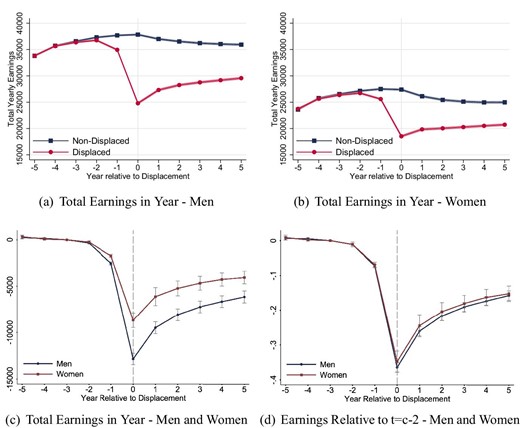
The gender gap in earnings losses after displacement without controlling for pre-displacement characteristics. The figures show earnings losses for displaced and non-displaced workers. Panels (a) and (b) show total yearly earnings for displaced and non-displaced men (a) and women (b). The red line corresponds to workers who are displaced from year t = c-1 to t = c, while the blue line corresponds to the matched control group that is constructed of non-displaced workers via propensity score matching. Each point represents the average value in the respective worker group. Panels (c) and (d) show event study coefficients, controlling for person FE, year FE, years since separation, and age polynomials. Panel (c) shows event study coefficients for total yearly earnings as outcome. Panel (d) shows event study coefficients for earnings relative to t = c−2 as outcome. The red line corresponds to women, the blue line corresponds to men. Workers are displaced in 2002–2012, and they are observed from 1997 to 2017.
Panel (c) plots the event study coefficients from equation (5) for annual earnings in levels. Given the matching design, the additional controls make virtually no difference and the event study coefficients are very close to the simple difference in the means of the two lines in Panels (a) and (b). This figure shows that in levels, women have substantially smaller losses of around 9,000 Euro in the first post-displacement year, while men lose around 13,000 Euro. The recovery path looks similar, but even 5 years out women’s losses are smaller. The higher losses in levels stem largely from the fact that men have more to lose given their higher baseline earnings. Panel (d) thus shows the earnings losses using as an outcome earnings in the respective year divided by each individual’s earnings in year t = c − 2, that is, the year before the baseline year, we denote this as |$\tilde{y}_{i,t}\equiv y_{i,t}/y_{i,c-2}$|. This outcome variable has the distinct advantage that it expresses the effect in percentage terms, allows the inclusion of 0 earnings, and is straightforward to interpret.
Figure 1(d) reveals that in percentage terms men and women in this unweighted sample experience virtually identical relative earnings losses and recovery paths. Furthermore, the magnitudes are large: In the first year, earnings decline by almost 40% relative to pre-displacement earnings. In the following years, there is some recovery, but 5 years out earnings are still about 20% lower relative to the pre-displacement year.
Table 2 shows the corresponding estimates from our matched difference-in-difference design, that is estimates of equation (6). The unit of observation in this regression is displaced workers, where for each displaced worker we calculated Δddyic for various outcomes. Each row corresponds to a different outcome variable. Column (1) shows the mean change in the outcome variable for men and column (2) shows the unadjusted gender gap from estimating equation (6).
The gender gap in earnings losses and other characteristics after displacement.
| (1) | (2) | (3) | (4) | ||||
| Mean change | Unadjusted | Composition | Number of | ||||
| in outcome variable | gender | adjusted gender | observations | ||||
| for men | gap | gap reweighted | |||||
| Change | Std. err. | Gap | Std. err. | Gap | Std. err. | ||
| Panel A: Earnings, wages, and employment | |||||||
| Total yearly earnings | −9418.0 | [313.8] | 3214.6 | [371.2] | −2491.1 | [339.6] | 80,655 |
| Earnings r.t. t = c−2 | −0.258 | [0.0066] | 0.014 | [0.012] | −0.092 | [0.012] | 80,655 |
| Log earnings | −0.405 | [0.0077] | −0.030 | [0.020] | −0.128 | [0.017] | 76,321 |
| Log wage loss | −0.201 | [0.0053] | −0.066 | [0.013] | −0.133 | [0.013] | 73,598 |
| Fulltime log wage | −0.094 | [0.0029] | 0.013 | [0.0085] | −0.039 | [0.0084] | 52,996 |
| Days worked | −67.7 | [2.01] | 9.04 | [2.97] | −7.05 | [2.13] | 80,655 |
| Days worked fulltime | −75.5 | [2.11] | 31.4 | [3.24] | −23.1 | [2.84] | 80,655 |
| Days worked parttime | −0.154 | [0.380] | −33.8 | [1.72] | 11.3 | [1.66] | 80,655 |
| Days worked in minijob | 1.09 | [0.516] | 14.3 | [1.10] | 4.88 | [1.51] | 80,655 |
| Panel B: Job characteristics | |||||||
| Commuting distance | 2.59 | [1.54] | −8.76 | [1.62] | −0.321 | [2.11] | 73,027 |
| Log establishment size | −0.740 | [0.029] | −0.571 | [0.077] | −0.041 | [0.036] | 72,811 |
| Industry change | 0.536 | [0.0066] | −0.061 | [0.020] | 0.046 | [0.011] | 73,564 |
| Occ. change | 0.417 | [0.0067] | −0.105 | [0.015] | −0.043 | [0.012] | 73,598 |
| Estab share women | 0.019 | [0.0024] | 0.019 | [0.0032] | 0.042 | [0.0049] | 72,370 |
| Temp work | 0.034 | [0.0014] | −0.012 | [0.0018] | −0.0087 | [0.0026] | 72,811 |
| Business service estab | 0.064 | [0.0023] | −0.019 | [0.0032] | −0.028 | [0.0040] | 72,811 |
| New estab | 0.195 | [0.0067] | 0.085 | [0.018] | 0.0063 | [0.0087] | 72,811 |
| AKM estab FE | −0.086 | [0.0063] | 0.011 | [0.0066] | −0.0097 | [0.0054] | 63,452 |
Notes: Each row represents a separate regression of the mean change in the outcome variable over a 5-year period after job loss on a constant and a dummy for female. The first column shows the constant, representing the mean effect for men. The second column presents the coefficient on a female dummy without any controls. The third column presents the coefficient on the female dummy controlling for all covariates. The fourth column uses reweighting. We cluster standard errors at the displacement establishment level (constant within matched worker pairs). Sinh(Earnings) refers to the inverse hyperbolic sine transformation of earnings. We measure commuting distance as the kilometer distance between two municipality centroids. Industry and occupation changes are defined on the 2-digit and 3-digit levels, respectively. “Temp Work”, “Business Service Estab.”, and “New Estab.” are variables indicating whether workers changed their job to temporary work, to a business service establishment, or to a new establishment (5 years old or younger), respectively. Workers in our sample are displaced in 2002–2012, and they are observed from 1996 to 2017. Coefficients in bold are statistically significant at the 5%-level.
The results in columns (1) and (2) confirm the impression from Figure 1. Men experience large earnings losses both in levels (around 9,400 Euro per year) and relative to the baseline (around 26%). For women, the earnings losses are smaller in levels (a loss of about 6,200 Euro per year), but very similar in relative earnings or when using log earnings.
Overall, there are large earnings losses that are comparable to estimates for Germany (Schmieder, von Wachter, and Heining 2023) or the U.S. (e.g. Jacobson, LaLonde, and Sullivan 1993; Couch and Placzek 2010; or Lachowska, Mas, and Woodbury 2020). Bertheau et al. (2023) estimate displacement effects for a range of countries and show in their Appendix Figure A.2 earnings losses separately by gender (in this case without adjusting for pre-displacement job differences between men and women). The figures look very similar to our Figure 1(d) with large but very similar losses for men and women. There is also substantial heterogeneity in the overall losses by country with Germany looking similar to Austria and somewhat in the middle between the large losses in Southern Europe and the much smaller losses in Northern Europe and France.
3.2. The Gender Gap in Earnings Losses for Men and Women Displaced from Comparable Jobs
We now turn to estimating the gender gap in earnings losses when we compare women who are displaced from comparable jobs as men using the reweighting technique described in Section 2.4.
Figure 2 shows event study graphs for various outcomes with and without reweighting. Each panel shows three lines: the event study estimates for men (solid blue line), for women without reweighting (solid red line), and for women reweighted to the job characteristics of men. Figure 2(a) shows a striking result: while earnings losses for our broad sample of women were very similar than for men, once we reweight women to closely match the men, their earnings losses become much larger: Women lose about 5 percentage points more earnings immediately after job loss and the gap grows over time to around 15 percentage points 5 years after job loss. Online Appendix Table C.10 shows how the gender gap in earnings losses changes as we include reweighting variables one by one. The full-time employment dummy and the establishment characteristics play a particularly important role.
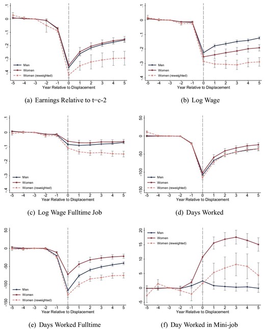
The gender gap in earnings, wages and employment losses after displacement, controlling for pre-displacement characteristics. This figure shows how earnings losses, wage losses and losses in days worked from displacement differ for men and women. Panels (a)–(f) show event study coefficients for log wage, log wage from full-time jobs, earnings relative to 2 years before displacement, days worked, days worked in full-time job, and days worked in minijob. The three lines correspond to three event study regressions: Men only, women only, and women reweighted with individual and establishment characteristics. All regressions include controls for person FE, year FE, years since separation, and age polynomials. Vertical bars indicate the estimated 95% confidence interval based on standard errors clustered at the individual level. Workers are displaced in 2002–2012, and they are observed from 1997 to 2017.
Table 2, column (3) shows regression estimates of the gender gap when accounting for differences in job characteristics between women and men. The first row shows that when controlling for observables, women lose around 2500 Euro more in annual earnings, which amounts to a relative earnings loss that is 9.2 percentage points larger for women than for men (row 2), closely in line with the reweighted event study results from Figure 2(b). We find similarly large gender gaps when looking at log earnings.
3.3. The Role of Wage and Employment Losses after Job Displacement
Earnings losses after job loss occur partly due to workers being unemployed or leaving the labor force, and partly due to losses in wages and hours worked. While the German social security data does not contain information on hours worked, it has detailed information on annual days worked and it provides an indicator for whether workers are working full-time, part-time, or in a mini-job. There is no information on hourly wages, but we can compute daily wages and daily wages conditional on working in a full-time job.
Figure 2 Panel (b) shows that log daily wages decline dramatically after job loss for both men and women. Even unweighted, women have larger losses in daily wages but this gap becomes much larger when reweighting women to their male counterparts and women lose around an extra 8 log points immediately after displacement, a gap that grows to around 20 log points 5 years out. Turning to full-time log wages in Panel (c), we find that men and women experience similar losses without weighting, but there is again a very substantial gender gap once we reweight women to match the men. Overall women lose about an extra 5 log points conditional on working full-time.
Panel (d) shows that women have similar employment losses to men when measured as annual days worked. This, however, masks a large composition-adjusted gap in days worked full-time (Panel e) when comparing similar men and women, where women work around 30 days less full-time per year.17 This implies that women are much more likely to take on part-time jobs than men and indeed even women who worked full-time before often switch to working part-time afterward, something rarely observed for men (for results on part-time employment, see Online Appendix Figure C.5(e)).
This is also supported by Panel (f), which shows the number of days worked in a mini-job. While a part-time job is any job with less than 25 hours of work per week, mini-jobs are a special type of marginal employment in the German labor market. For most of our observation period, mini-jobs can pay at most 400 Euros per month.18 They are exempt from social security contributions and are particularly common among female workers, partly because they make it easy to combine work and family life. Note that given our baseline restrictions, we exclude workers working only in mini-jobs pre-displacement, though they can work a mini-job on the side. Following job loss, there is essentially no uptake of mini-jobs for men, however, there is a big increase for the broad sample of women of around 15 days, and about an 8 day increase after reweighting. In fact, the large increase in part-time and mini-jobs for women after displacement is an important factor behind the large daily wage losses for women in Panel (b) compared to men.
The visual results from Figure 2 are also confirmed in Table 2. Overall, holding pre-displacement characteristics constant, women experience much larger employment losses than men, are more likely to switch to part-time work or mini-jobs, and have larger wage losses, even when conditioning on working full-time. All factors together produce the large and lasting earnings losses that we documented in Section 3.2.
4. Understanding the Gender Gap in Wage Losses
4.1. Changes in Job and Establishment Characteristics after Job Displacement
The previous section showed that there is a large gender gap in earnings and wage losses for displaced women compared to men. Yet, how does the nature of jobs change after displacement?
Figure 3(a) and (b) show the probability of switching industry or occupation, which previous papers have highlighted as an important channel for wage losses after displacement since they are usually correlated with losses in human capital (e.g. Topel 1990; Neal 1995). Approximately 30% of job losers switch industries and about 40%–50% switch occupations immediately after job loss. Gender differences here are pretty modest, especially after reweighting. In fact, women are slightly less likely to switch occupations. We do however find that if we use average occupation wages as an outcome, women lose slightly more than men (Online Appendix Figure C.5(f)).
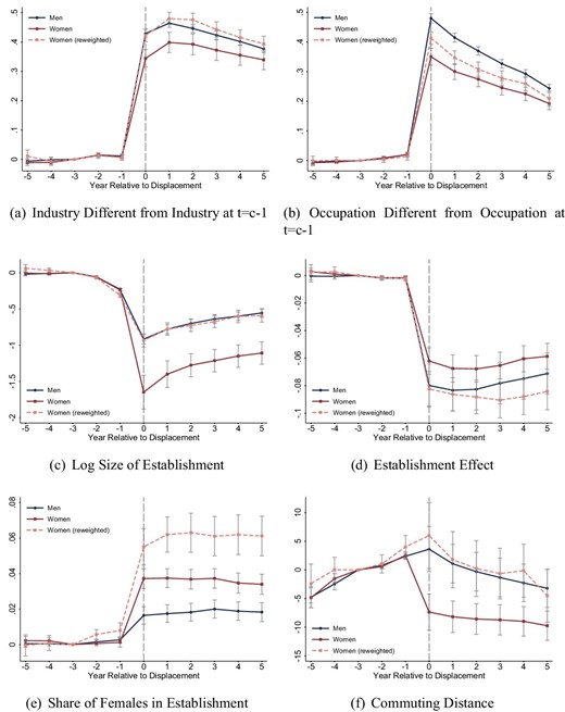
Changes in job characteristics after displacement. This figure shows how job characteristics for men and women evolve before and after displacement. Panels (a)–(f) show event study coefficients for industry switches (2-digits), occupation switches (3-digits), log establishment size, AKM establishment effects, the share of female workers in the establishment (leave-one-out mean), and commuting distance (in km). The three lines correspond to three event study regressions: Men only, women only, and women reweighted with individual and establishment characteristics. All regressions include controls for person FE, year FE, years since separation, and age polynomials. Vertical bars indicate the estimated 95% confidence interval based on standard errors clustered at the individual level. Commuting distance is measured on the municipality level, and is recorded on December 31 each year. Workers are displaced in 2002–2012, and they are observed from 1997 to 2017.
As one measure of employer quality, we show log establishment size in Figure 3(c). Recall from Table 1 that women tend to work at larger establishments before reweighting. In this broad sample, women move to much smaller establishments post-displacement. However, after reweighting the difference disappears.
A more direct measure of employer quality are estimated establishment fixed effects from an AKM model (Abowd, Kramarz, and Margolis 1999). A recent version of the AKM model for our time period was estimated by Lochner, Wolter, and Seth (2023), who generously made their estimates available to us. Figure 3(d) shows the evolution of the estimated establishment effect after job loss. The estimated establishment effect drops by around 8 log points for men. This corresponds almost exactly to the drop in log full-time wages for men, confirming the result in Schmieder, von Wachter, and Heining (2023) that the change in establishment effects fully accounts for the change in log wages for displaced men for a slightly earlier time period. For women, the unweighted loss in the establishment effect is slightly smaller than for men, with around 6 log points losses, while after reweighting the loss is larger, around 9 log points in year 5. These establishment effect losses mirror the losses in log full-time wages for women in Figure 2(b) and suggest that at least part of the gender gap in log full-time wages (and thus earnings) is due to women moving to worse-paying firms relative to men after job loss.
As another measure of establishment characteristics, we show the share of women working in an establishment as an outcome variable in Panel (e). The figure shows that while the share of female coworkers remains similar for men after displacement, women move to establishments with much more female coworkers. Unweighted, women move to establishments with a female share that is 4 percentage points higher, while after weighting this increases to around 6 percentage points. Strikingly, this suggests that even women with similar careers as men fall back to more typical female employers. This complements the evidence on the establishment wage premiums, and is consistent with the evidence from Card, Cardoso, and Kline (2016) that women tend to be concentrated in low-paying establishments.19
Finally, Figure 3(f) shows how commuting distances are affected by job loss. Our measure of commuting distance (in km) is the straight line distance between the geographic center of the municipality of residence and the municipality of work. The result on the broad sample of women is in line with Le Barbanchon, Rathelot, and Roulet (2021), showing that women substantially reduce commuting distance after job loss, by almost 8 km (relative to a 30 km commute prior to displacement), while men’s commuting distance is essentially unchanged. However, when we reweight women to match men, the gap in commuting disappears completely and women’s commutes remain unchanged relative to their pre-displacement job.
4.2. Sources Underlying the Gender Gap in Wage Losses
Given the changes in job characteristics shown above, we turn to whether these observable post-displacement job characteristics can explain the losses in wages and the gender gap in particular. For this, we estimate equation (7), including changes in job characteristics ΔddZic as explanatory variables. Table 3 shows these estimates both for overall daily wages (Panel A) and full-time wages (Panel B). All regressions are weighted so that women match their male counterparts. Column (1) reproduces the benchmark results from Table 2, column (3) for the two outcomes.
Explaining the gender gap in wage losses after displacement.
| (1) | (2) | (3) | (4) | |
|---|---|---|---|---|
| OLS | Kitagawa–Oaxaca–Blinder decomp. | |||
| Endowments | % Explained | |||
| Panel A: All workers: Log wage | ||||
| Female | −0.13 | −0.096 | ||
| (0.013)** | (0.011)** | |||
| Part-time job | −0.17 | −0.0084 | 6.31 | |
| (0.018)** | (0.0012)** | (0.90)** | ||
| Mini-job | −0.70 | −0.0079 | 5.91 | |
| (0.026)** | (0.0024)** | (1.81)** | ||
| Industry change | −0.090 | −0.0033 | 2.49 | |
| (0.010)** | (0.00083)** | (0.62)** | ||
| Occ. change | −0.082 | 0.0028 | −2.12 | |
| (0.0084)** | (0.00081)** | (0.61)** | ||
| Log estab size | 0.036 | −0.0013 | 0.96 | |
| (0.0032)** | (0.0012) | (0.93) | ||
| Estab share women | −0.22 | −0.0089 | 6.71 | |
| (0.027)** | (0.0012)** | (0.94)** | ||
| Commut. distance | −0.000069 | −0.0000017 | 0.0013 | |
| (0.000060) | (0.000016) | (0.012) | ||
| AKM estab FE | 0.83 | −0.0066 | 4.94 | |
| (0.057)** | (0.0039) | (2.90) | ||
| Observations | 73598 | 73598 | ||
| R2 | 0.010 | 0.319 | ||
| Mean dep. var men | −.201 | −.201 | ||
| (.003) | (.003) | |||
| Total gap | −0.13 | 100.0 | ||
| (0.016)** | (11.8)** | |||
| Explained gap | −.035 | 26.258 | ||
| Panel B: Full-time workers: Full-time log wage | ||||
| Female | −0.039 | −0.030 | ||
| (0.0084)** | (0.0076)** | |||
| Industry change | −0.031 | −0.0011 | 2.86 | |
| (0.0067)** | (0.00040)** | (1.02)** | ||
| Occ. change | −0.0096 | 0.00059 | −1.51 | |
| (0.0054) | (0.00021)** | (0.53)** | ||
| Log estab size | 0.012 | 0.000018 | −0.045 | |
| (0.0018)** | (0.00040) | (1.03) | ||
| Estab share women | −0.056 | −0.0012 | 3.18 | |
| (0.016)** | (0.00032)** | (0.81)** | ||
| Commut. distance | 0.000054 | 0.000028 | −0.072 | |
| (0.000040) | (0.00015) | (0.39) | ||
| AKM estab FE | 0.70 | −0.0072 | 18.2 | |
| (0.055)** | (0.0035)* | (9.01)* | ||
| Observations | 52,996 | 52,996 | ||
| R2 | 0.003 | 0.228 | ||
| Mean dep. var men | −.094 | −.094 | ||
| (.002) | (.002) | |||
| Total gap | −0.039 | 100.0 | ||
| (0.014)** | (35.4)** | |||
| Explained gap | −.009 | 22.492 | ||
Notes: This table shows to what extent changes in contract type, industry, occupation, and establishment characteristics can explain the effect of being female on wages after displacement. All outcome variables are based on the individual difference-in-differences estimate. In all columns, we reweight women to men using individual and establishment characteristics pre-displacement. The coefficients in columns (1)–(3) are estimated from OLS regressions. In column (3), the coefficient on the AKM establishment effect is forced to be equal to 1. Column (4) shows the explained part, or endowment effects, from a Kitagawa–Oaxaca–Blinder decomposition, corresponding to |$(E(X|\textit{female})-E(X|\textit{male}))\beta _{\textit{male}}$|. Column (5) shows the % of the total wage gap explained by each variable. Workers in our sample are displaced in 2002–2012, and they are observed from 1996 to 2017. Standard errors (in brackets) are clustered at the displacement establishment level (constant within matched worker pairs). * and ** correspond to 5% and 1% significance levels, respectively.
Column (2) shows how the gender gap decreases when controlling for changing job characteristics. These include changes in industry and occupation, differences in employment size, the establishment share of women, commuting distance, and changes in the AKM establishment fixed effect. In addition, we also include switches to part-time and mini-jobs in Panel (A). The various job characteristics show the expected signs: switching to part-time (mini-job) is associated with a 17 (70) log point loss in wages, industry and occupation changes are associated with a loss of 8–9 log points in wages, and going to establishments that are smaller or have a larger share of female workers reduces wages. The AKM effect also has a clear negative effect, close to the theoretically expected value of 1.20 The inclusion of these controls reduces the gender gap in wage losses from 13 to 9.6 log points or by about 25%.
Based on Le Barbanchon, Rathelot, and Roulet (2021), we might expect that women trade-off a higher wage for a shorter commute after job loss and that this would explain some of the gender gap, however, we find no clear evidence of this either for wage losses.
To better understand how much each of the job characteristics explains the gender gap in earnings losses, we turn to a Kitagawa–Oaxaca–Blinder decomposition in columns (3) and (4). For this, we estimate the wage loss model separately by gender and then compute the part of the wage loss that is explained by gender as |$(\bar{X}_{\textit{female}}-\bar{X}_{\textit{male}})\beta _{\textit{male}}$|. Column (3) shows these endowment contributions for each variable, while column (4) expresses the contribution in percent of the total gender gap in earnings losses. Interestingly the most important factor is the share of women at the employing establishment, which explains almost 7% of the gender gap. Part-time and mini-job status explain just a little bit less (around 6%) and occupation goes in the opposite direction (women are less likely to switch occupations). The AKM effect explains about 5% of the gap but is imprecisely estimated.
Panel B does the same analysis but restricting observations to workers working full-time (before and after job loss). We can explain 22.5% of the gender gap with the observables. Interestingly, by far the most important job characteristic is the AKM establishment effect of the employer, which explains about 18% of the gap. Given that the AKM model is geared toward capturing the establishment wage premia for full-time workers, it is not surprising that its explanatory power is much larger for log wages of workers remaining in full-time employment.
4.3. The Role of Children
Are the earnings losses after displacement affected by whether young children are in the household? Ex-ante one can imagine different channels for why children may matter. On the one hand, holding income constant, the presence of children may increase the marginal value of consumption since household income is spread thinner. This may increase search effort during spells of unemployment following job loss or increased hours worked once a job is found. On the other hand, the presence of children may increase the opportunity cost of working. Especially if there is a permanent loss in wage prospects for job losers, as we showed in Section 3.3, this may make it relatively more attractive to focus on childcare instead of labor market participation.
To estimate the effect of job displacement separately by the age of the youngest child in the household, we extend the model in equation (6):
where |$\textit{KidAge}_{i}$| is the age of the youngest child of the displaced worker (or an indicator if there is no child) and a indicates the possible age of the youngest child. The covariates Xi are demeaned, so that the estimated αa provide estimates of the cost of job loss for men with a child aged a (or no child), while the estimated βa provide the respective gender age gap.21
Figure 4 plots the estimated effects for men αa and for women (αa + βa). We plot the estimates for men and women without children on the far right of the graph. Panel (a) shows our main outcome: earnings relative to t = c − 2. For men and women without young children, the results confirm those in Section 3.3: women have significantly larger earnings losses than men when holding pre-displacement characteristics constant. A striking result emerges, however, when comparing these with parents: displaced men who have a child at home have smaller earnings losses than men without young children. In stark contrast, mothers of very young children have much larger earnings losses in the order of 60% of pre-displacement earnings. Mothers with older children (around 3 years and older) have comparatively much smaller earnings losses, albeit still larger than men. We observe a similar pattern for log wages in Panel (b). A plausible explanation for the trend break at age 3 might be that this is when children typically enter kindergarten and then elementary school, in effect reducing the opportunity cost of working.
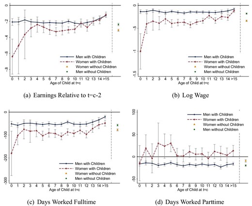
The gender gap and children. This figure shows how labor market outcomes before and after displacement differ for men and women by age of the youngest child at the time of displacement. All outcome variables are the respective difference-in-difference estimate. Panels (a)–(d) show event study coefficients for earnings relative to t = c−2, log wage, days worked in a full-time job, and days worked in a part-time job. The dark blue line corresponds to men with children, the dashed red line corresponds to women with children. The green diamond and orange triangle report coefficients for men without children and women without children, correspondingly. All regressions control for individual and establishment characteristics. Individual characteristics are a worker’s log wage in t = c−3 and t = c−4, full-time employment in t = c−3, and age, years of education, tenure, and location in East or West Germany in t = c−1. Establishment characteristics are 1-digit industry dummies and log establishment size in t = c−1. Vertical bars indicate the estimated 95% confidence interval based on standard errors clustered at the displacement establishment level. Workers are displaced in 2002–2012, and they are observed from 1997 to 2017.
Panels (c) and (d) show that women with very young children also have huge losses in days working full-time without a parallel increase in working part-time. However, once children are 3 or older, there appears to be more of a substitution effect from full-time to part-time rather than dropping out of the labor force.
Interestingly, for mothers with teenage children, the gap largely disappears. Note, that we can only observe children who are born while the mother is employed so that the ‘without children’ group likely also contains some mothers whom we misclassify. Thus one possibility might be that the gender gap for childless job losers is in fact 0 (as the figure suggests for parents with children older than 15), and that the gender gap is entirely driven by mothers.22
Table 4 shows comparable results from a regression model, where we estimate equation (7) but include dummies for children younger than 16, both interacted with gender. The omitted category is men without children. The results suggest that for job losers without children, there is still a gender gap but only 3.9 percentage points, and thus less than the overall gender gap. The coefficient on the dummy for child (0.0096) and its interaction with a female dummy (−0.021) show that the presence of young children substantially reduces the earnings losses for men, but sharply increases earnings losses for women.
The gender gap in labor market outcomes by household characteristics.
| (1) | (2) | (3) | (4) | (5) | (6) | |
|---|---|---|---|---|---|---|
| Earnings | Log | Days | Commuting | Estab FE | Partner’s | |
| rel. to | wage | worked | distance | earn. rel. to | ||
| t = −2 | job loser’s | |||||
| Panel A: Regression adjusted gender wage gap—adding family controls | ||||||
| Female | −0.039 | −0.14 | 0.65 | −3.46 | −0.018 | −0.034 |
| (0.0080)** | (0.011)** | (1.83) | (1.46)* | (0.0048)** | (0.0091)** | |
| Child | 0.0096 | 0.015 | 2.55 | −0.77 | 0.0088 | 0.011 |
| (0.0039)* | (0.0047)** | (1.05)* | (0.85) | (0.0023)** | (0.0036)** | |
| Female*Child | −0.021 | −0.020 | −2.86 | 0.67 | −0.011 | −0.013 |
| (0.0078)** | (0.0091)* | (1.95) | (1.33) | (0.0037)** | (0.015) | |
| Observations | 161,310 | 147,196 | 161,310 | 146,054 | 126,904 | 161,310 |
| R2 | 0.030 | 0.034 | 0.025 | 0.027 | 0.057 | 0.002 |
| Mean dep. var men | −.258 | −.201 | −67.66 | 2.59 | −.086 | −.02 |
| (.002) | (.002) | (.414) | (.312) | (.001) | (.003) | |
| Panel B: Regression adjusted gender wage gap—adding household income controls | ||||||
| Female | −0.055 | −0.15 | −3.21 | −3.32 | −0.024 | −0.035 |
| (0.0077)** | (0.011)** | (1.81) | (1.47)* | (0.0049)** | (0.011)** | |
| Earn. share in HH Inc. | −0.029 | −0.036 | −6.93 | −0.44 | −0.0050 | 0.052 |
| (0.013)* | (0.014)** | (2.90)* | (3.26) | (0.0078) | (0.015)** | |
| Female*Earn. share | −0.0013 | 0.015 | −6.92 | −0.64 | −0.0055 | 0.0030 |
| (0.019) | (0.022) | (4.29) | (3.65) | (0.010) | (0.039) | |
| Observations | 126,151 | 115,338 | 126,151 | 114,466 | 98,161 | 126,151 |
| R2 | 0.034 | 0.036 | 0.028 | 0.026 | 0.057 | 0.002 |
| Mean dep. var men | −.258 | −.201 | −67.66 | 2.59 | −.086 | −.02 |
| (.002) | (.002) | (.414) | (.312) | (.001) | (.003) | |
Notes: This table shows the role of children and household dynamics in explaining gender-specific labor market outcomes after displacement. All outcome variables are based on the individual difference-in-differences estimate. Panel (A) shows the regression-adjusted gender gap controlling for having children younger than 16. In Germany, children enter school aged 6–7. Panel (B) adds shows the regression-adjusted gender gap controlling for the job loser’s earnings share in household income measured in t = c−1. The share in household income is set to missing if the partner is not working. We cluster standard errors at the displacement establishment level (constant within matched worker pairs). Workers in our sample are displaced in 2002–2012, and they are observed from 1996 to 2017. * and ** correspond to 5% and 1% significance levels, respectively.
The remaining columns of Table 4, as well as the other panels of Figure 4, complete the story: The presence of children has a positive effect on men’s post-displacement trajectories: they work more, have lower wage losses, show a higher probability of working full-time. For women, the effects are reversed with larger losses in days worked and wages. Women also move to lower-paying employers if they have young children. Interestingly, mothers of young children also have a pretty large (though statistically insignificant) decline in commuting distances after displacement, potentially to be able to better reconcile childcare with work.
A question that we cannot answer well in the IAB data (where births are only observed for working mothers) is whether women decide to have children in response to a layoff and whether this could lead to larger earnings losses for women. However, the existing evidence from other countries would speak against the hypothesis that women have children in response to being laid off. For example, Del Bono, Weber, and Winter-Ebmer (2012) and Huttunen and Kellokumpu (2016) both find negative fertility effects for women (and small or no effects for men).
4.4. The Role of Within-Household Earnings Inequality
Ex-ante it seems plausible that whether the job loser was the main breadwinner (that is, contributing more than 50% of household income) or just a small contributor, may affect post-displacement outcomes. For example, the higher the within-household income share of the displaced worker the larger the shock to the household finances.23 Moreover, gender identity norms, as in Bertrand, Kamenica, and Pan (2015), could make it undesirable for either or both partners that the wife makes more money than the husband. In this case, the pre-displacement within-household income distribution may be an important determinant for post-displacement outcomes.
In Table 4, Panel B, we show estimates of our main regression equation (6) where we add the share of household income of the job loser both by itself and interacted with the female dummy. A simple interpretation of Bertrand, Kamenica, and Pan (2015) would be that having a higher share of household income is associated with higher earnings losses for women relative to men (and thus a negative coefficient on the interaction term in column (1)). However, while earnings losses become larger with a larger earnings share of the displaced worker, the effect is very small (an increase in the earnings share by 0.1 implying a 0.3 percentage point larger earnings loss) and the effect seems virtually identical for men and women. Similar patterns hold for wages and employment.
A more nuanced view of Bertrand, Kamenica, and Pan (2015) would, however, suggest that the effect may be nonlinear: if women (or their spouses) have a strict preference to make less money than their husbands, then losses should be highest for women who make significantly more than their husband and who may actually move to a less than 50% household share post-displacement. However, for everyone close to 50% pre-displacement earnings no such motivation exists and the household share should not affect earnings losses through the gender identity channel.
To capture this nonlinearity, Online Appendix Figure C.4 shows the effects of displacement on earnings losses by bins of pre-displacement household income share. In this figure, male earnings losses are not much affected by their share of household earnings, but female earnings losses show some non-linearity and resemble an inverse U-shape with the lowest earnings losses close to earnings parity between both spouses, and a slight decline if women have a higher household income share (though note that we have few observations where women have a substantially larger than 50% share of household income). Interestingly, for low income shares, women’s earnings losses also become larger. This might be because their income is relatively less important to the financial situation of the household, making dropping out of the labor force or working part-time to look after children potentially more appealing. This impression is even stronger when looking at days worked full-time and part-time. Overall, this may be viewed as weak evidence in support of the identity model in Bertrand, Kamenica, and Pan (2015).
An additional question related to the household level is whether the losses on the household level are larger when the husband or the wife loses their job. Given the literature on the added worker effect (Lundberg 1985; Halla, Schmieder, and Weber 2020), it seems possible that the losses of a male job loser are more likely to be compensated to some extent by additional labor supply of his wife, compared to the other way around. Our context is not ideal for studying the added worker effect due to the restriction that we can only observe couples where both partners are in the labor force, but we provide some analysis of this in column (6), where we show the effect on partner earnings. Note that partner earnings decline for men and women. In Online Appendix Tables C.5 and C.6, we present results that the absence of an added worker effect is likely due to correlated economic shocks since many spouses work in the same industry or firm. Furthermore, declines in total household earnings are similar for male and female job losers after adjusting for observables, where the larger earnings losses for women are weighed against higher household income shares for men.
4.5. Labor Supply or Labor Demand? Gender Differences in Job Preferences and Job Search Behavior after Job Loss
The gender differences in labor market outcomes after job loss beg the question of whether they are due to differences in labor supply or labor demand. For example, the labor supply channel may operate through women searching less for a job (e.g. because of increased childcare duties at home) or wanting to work fewer hours after a job loss, in comparison to men. On the other hand, the labor demand channel may operate through women facing discrimination by potential employers; thus, having a harder time than men recovering from job loss.
Job Seekers in Baseline Displaced Worker Sample.
While we cannot fully disentangle these two channels, we leverage two additional data sources to shed some light on what is arguably the labor supply side. First, we use self-reported job search preferences for workers in our sample, which we obtained from the UI system (so-called “ASU” data). Workers who are displaced typically have contact with the UI system soon after being notified of the upcoming layoff (the employer has to notify the UI agency in advance of a mass layoff). If they are assigned a caseworker to assist with job search, the worker fills out several questions regarding what type of employment he or she is looking for and what the scope of the search is. In our sample, about 70% of displaced workers register as job searchers in the year of the mass layoff and we have valid information on job preferences for about 53,000 individuals in our sample.24Online Appendix Table C.7 shows that along observable characteristics workers with ASU information look very similar to the full sample of workers, with the main difference being that earnings are about 6% lower.
The key variables we focus on are whether a worker is looking only for a full-time job (as opposed to part-time or full- or part-time); whether or not a worker is looking broadly in terms of geography (i.e. willing to commute significantly or move); and whether a worker is looking for a permanent (i.e. open-ended) contract as opposed to a fixed-term contract.
Table 5 presents this information in the same format as Table 2 with the difference that in this table, we only use post-displacement outcomes for displaced workers, since these outcomes are naturally not available for non-displaced workers and prior to job loss. Panel A shows quite strikingly that 98% of men are looking only for a full-time job (column 1), in contrast to women where less than 70% are only looking to work full-time in the overall sample (column 2). After controlling for observables (column 3), the gender gap shrinks but women are still about 11 percentage points less likely to look for a full-time job, despite the fact that in this reweighted sample almost all women were working full-time before. Looking at the geographic dimension of job search, we see that women are about 4 percentage points less likely to search broadly (40% compared with 44%), which shrinks to around 2 percentage points after adjusting for observables. The table also shows that women are somewhat less likely to look for permanent contracts.
Gender differences in job preferences and search behavior after job loss.
| (1) | (2) | (3) | (4) | (5) | ||||
| Mean outcome | Unadjusted | Composition | Number of | Data | ||||
| men | gender gap | adjusted gender | observations | source | ||||
| gap reweighted | ||||||||
| Change | Std. err. | Gap | Std. err. | Gap | Std. err. | |||
| Panel A: All | ||||||||
| Searching f. full-time job | 0.979 | [0.0016] | −0.314 | [0.0061] | −0.113 | [0.0060] | 45,087 | ASU |
| Broad geographic search | 0.439 | [0.0051] | −0.040 | [0.0073] | −0.019 | [0.012] | 31,349 | ASU |
| Permanent contract | 0.745 | [0.0075] | −0.035 | [0.0091] | −0.0066 | [0.010] | 45,131 | ASU |
| Minutes job search | 94.0 | [1.62] | −18.0 | [2.09] | −9.18 | [2.68] | 116,159 | SMS |
| Target wage ratio | 1.17 | [0.016] | 0.077 | [0.023] | −0.054 | [0.027] | 5,541 | SMS |
| Life satisfaction (Scale 1–5) | 2.99 | [0.022] | 0.117 | [0.031] | 0.154 | [0.039] | 14,158 | SMS |
| Panel B: Age Youngest Child ≤15 | ||||||||
| Searching f. full-time job | 0.980 | [0.0018] | −0.557 | [0.011] | −0.258 | [0.018] | 13,292 | ASU |
| Broad geographic search | 0.444 | [0.0072] | −0.048 | [0.013] | −0.069 | [0.028] | 8,938 | ASU |
| Permanent contract | 0.739 | [0.0086] | −0.083 | [0.013] | −0.100 | [0.024] | 13,223 | ASU |
| Minutes job search | 91.5 | [3.37] | −22.2 | [3.94] | −14.8 | [4.91] | 30,582 | SMS |
| Target Wage Ratio | 1.20 | [0.031] | 0.132 | [0.044] | −0.037 | [0.064] | 1,607 | SMS |
| Life Satisfaction (Scale 1–5) | 3.08 | [0.050] | 0.142 | [0.062] | 0.166 | [0.079] | 3,663 | SMS |
Notes: Each row represents a separate regression of the outcome variable on a constant and a dummy for female for a sample of displaced workers, only. In Panels B and C, we restrict the sample to individuals with young children ≤ the age of 15 and above the age of 15, respectively. Data source ASU refers to the job-search preference data collected by the caseworkers at the local UI agency and is based on the subset of about 70% of workers in the baseline job-loss sample for whom this information is available. SMS refers to the high-frequency job-search data among unemployed workers between 2017 and 2019 as collected and described in DellaVigna et al. (2022), with the number of observations referring to the person × survey-date level. The first column shows the constant, representing the mean effect for men. The second column shows the coefficient on a female dummy without any controls. The third column shows the coefficient on the female dummy controlling for all covariates. The fourth column uses reweighting. We cluster standard errors at the displacement establishment level (constant within matched worker pairs). Workers in our sample are displaced in 2002–2012, and they are observed from 1996 to 2017. Coefficients in bold are statistically significant at the 5%-level.
UI Recipients Survey Data.
As a second data source, we use a survey of UI recipients by DellaVigna et al. (2022). The survey followed a sample of around 7,800 UI recipients over a period of 18 weeks and asked them regularly via text message (SMS) about the job search process. We focus on two questions: time spent on job search on the previous day in minutes (asked twice a week for the full survey length) and the approximate wage of the last job the person applied to, which we refer to as “target wage” (asked once every 4 weeks). The sample of the SMS survey does not overlap with our sample of job losers (the SMS survey was conducted between 2017 and 2019, while our job loss sample is restricted to job losses between 2002 and 2012). Online Appendix Table C.8 shows summary statistics for the SMS sample, highlighting that this group is of a similar age and gender composition as our main sample, but with about 1 year less education, lower wages, and shorter tenure duration. Despite these demographic differences (explained by the sampling frame of the SMS data), the individuals come from a similar context (German job losers) who lost somewhat stable jobs involuntarily.25 We restrict the sample to responses from individuals who were still unemployed on the date of their response, which yields a total of 116,159 valid responses to the time spent on job search question and 5,541 for the target wage. Table 5 shows that men spend on average 94 minutes on job search, while strikingly women only spend 76 minutes, or almost 20% less. After controlling for observables, the gap between men and women shrinks somewhat to around 9 minutes per day, still a 10% difference. In order to use the target wage as a measure for what type of jobs workers apply to, we divide it by the pre-unemployment wage. Our results show a target wage ratio of 1.17 for men, thus job seekers on average apply to jobs paying 17% more than their previous job. The target wage ratio for the average women in the sample is on average even higher, which appears to be due to the higher incidence of working part-time among women. However, after adjusting for observables, the target wage ratio falls significantly and is now about 5% lower than for men.
These results suggest that labor supply plays a significant role both for the raw and the composition-adjusted gender gap in post-displacement outcomes. For the raw gap, women are much less interested in full-time employment and show a narrower scope of job search (geographic and type of contract), they also spend much less time searching for a job, though they do report a slightly higher target wage ratio. For the composition-adjusted gap, women are still substantially less likely to look for a full-time job, have a narrower geographic scope, spend less time on search, and apply to lower-paying jobs (relative to pre-displacement).26 Of course, it should be noted, that while job search effort and scope is behavior on the supply side, this behavior itself may be driven by demand side factors. In particular women may face fewer suitable job options, for example, due to discrimination, which reduces the returns to job search or a broader scope of search.
The Role of Children for Job Preferences.
As discussed above, a driver for differences in labor supply could be the division of labor in households with children. In Panel B, we therefore show the analysis for workers with children (younger than 15). Men with children are very similar in terms of job preferences and job search behavior (column 1). In contrast, for women, the differences are quite stark. For the raw comparison, women with children are much less likely to search for a full-time job (compared to men but also to women without young children) and similarly have a narrower geographic scope of job search, and spend less time on job search. For the composition-adjusted gap, the differences are somewhat more muted, but women with children are still much less likely to look for full-time jobs, have a narrower scope of job search, and a lower target wage ratio. This further supports that the gender gap is at least in part driven by labor supply differences between men and women, possibly stemming from women being more likely to substitute child care for work in the labor market. It also highlights the importance of the job search process itself for shaping gender differences in labor market outcomes and is broadly consistent with the results in Le Barbanchon, Rathelot, and Roulet (2021) on commuting/wage trade-offs and the results in Cortes et al. (2022) on risk aversion and overconfidence. Again, it should be noted that these differences in labor supply behavior, may in part be driven by mothers facing fewer and worse job options, for example, because employers prefer hiring men or childless women to mothers.
5. Robustness of Main Results
Table 6 provides a range of robustness checks for our main results. For comparison, column (1) replicates the baseline estimates for the composition-adjusted gender gap for three key outcomes.
The gender gap in earnings losses—Robustness checks.
| (1) | (2) | (3) | (4) | (5) | (6) | (7) | |
|---|---|---|---|---|---|---|---|
| 10 years | Shorter | Reweight. | Displ. | Reweight. | Couples | ||
| Baseline | post displ. | tenure | with | estab. | men to | + | |
| restr. | occupations | FE | momen | non-couples | |||
| Panel A: Earnings rel. to year-2 | |||||||
| Female | −0.092 | −0.093 | −0.11 | −0.12 | −0.086 | −0.068 | −0.048 |
| (0.012)** | (0.018)** | (0.014)** | (0.025)** | (0.0089)** | (0.020)** | (0.013)** | |
| Observations | 80,655 | 55,107 | 93,755 | 80,423 | 77,144 | 78,695 | 96,158 |
| R2 | 0.007 | 0.006 | 0.008 | 0.013 | 0.352 | 0.003 | 0.002 |
| Mean dep. var men | −.258 | −.203 | −.268 | −.258 | −.258 | −.259 | −.287 |
| (.002) | (.003) | (.002) | (.002) | (.002) | (.002) | (.002) | |
| Panel B: Log wages | |||||||
| Female | −0.13 | −0.14 | −0.16 | −0.22 | −0.16 | −0.16 | −0.075 |
| (0.013)** | (0.017)** | (0.013)** | (0.036)** | (0.013)** | (0.017)** | (0.015)** | |
| Observations | 73,598 | 51,670 | 85,092 | 73,369 | 70,058 | 71,758 | 87,342 |
| R2 | 0.010 | 0.009 | 0.013 | 0.025 | 0.347 | 0.014 | 0.003 |
| Mean dep. var men | −.201 | −.187 | −.205 | −.201 | −.201 | −.202 | −.203 |
| (.003) | (.004) | (.003) | (.003) | (.003) | (.003) | (.003) | |
| Panel C: Days worked full-time | |||||||
| Female | −23.1 | −32.5 | −30.4 | −31.9 | −22.3 | −25.4 | −14.4 |
| (2.84)** | (3.73)** | (2.73)** | (6.66)** | (2.87)** | (4.64)** | (4.07)** | |
| Observations | 80,655 | 55,107 | 93,755 | 80,423 | 77,144 | 78,695 | 96,158 |
| R2 | 0.005 | 0.009 | 0.008 | 0.009 | 0.335 | 0.004 | 0.002 |
| Mean dep. var men | −75.47 | −56.298 | −77.46 | −75.471 | −75.47 | −75.664 | −84.705 |
| (.766) | (.976) | (.717) | (.766) | (.766) | (.765) | (.716) | |
Notes: Each column in this table represents a different robustness check. All specifications are estimated using weights. Column (1) reports the baseline coefficients. Column (2) reports results for a longer post-displacement time window (10 years). Column (3) reports results for shorter tenure workers (1 year at the time of displacement). Column (4) reports results when reweighting with 1-digit occupations in addition to industries and individual characteristics. Column (5) reports regression coefficients controlling for pre-displacement establishment fixed effects. Column (6) reports results when reweighting men to women. Trimmed at 99%. Column (7) reports regression coefficients for a combined dataset of couples and non-couples in our sample. We cluster standard errors at the displacement establishment level (constant within matched worker pairs). Workers in our sample are displaced in 2002–2012, and they are observed from 1996 to 2017. * and ** correspond to 5% and 1% significance levels, respectively.
Sample Construction.
While our baseline specification estimates the cost of job loss over a 5-year-horizon after displacement, Table 6, column (2) presents a result for a 10-year post-displacement horizon. Since we have to drop displacement events after 2007 to observe the full time horizon, we lose about 30% of our observations. Even over this longer time horizon results are very similar to before, suggesting that wage and earnings losses are highly persistent (see also Online Appendix Figure C.7 for event-study figures).
Our main estimates impose a 2-year tenure restriction in the baseline year. Column (3) shows that relaxing this restriction to only 1 year does not substantially alter the result. On the other hand, we show in Online Appendix Table C.14, column (6) that imposing the stricter restrictions (3 years tenure, baseline establishment size larger than 50) from Schmieder, von Wachter, and Heining (2023) leads to a larger gender gap.
Alternative Matching Algorithm.
In Online Appendix Table C.11, we provide a range of alternative specifications to create a matched control group, such as using Mahalanobis distance (instead of pscore) matching, using multiple control observations for each displaced worker, matching on more detailed industry and occupations, matching on county, AKM effects, and even just a simple random control group (without matching). The results are very similar across all specifications.
Alternative Reweighting Algorithm.
A key contribution of our approach is to hold pre-displacement characteristics constant when comparing men and women. Online Appendix Table C.17 shows that displaced women hold different pre-displacement occupations than men. For example, before the layoff displaced men often have blue-collar jobs, such as Trucker, Warehouseman, or Bricklayer and the broad white-collar occupation “Qualified Office Employee” only accounts for about 7.3% of job losers. Women on the other hand are much more likely to be in white-collar jobs with almost 40% being “Qualified Office Employees” or Salesperson. Table 6, column (5) shows that when we also reweight on 1-digit occupations, the gender gap becomes even larger, especially for wages. A downside of reweighting by occupation is that a small number of women then has to be upweighted to create a counterfactual for the many men in male-dominated occupations, which leads to larger standard errors. This becomes even more pronounced if we reweight using 2 digit occupations (see Online Appendix Table C.12, column 3, which shows even larger gaps but also much larger standard errors). We thus chose not to reweight by occupations as a conservative estimate of the gender gap. Similar results hold when reweighting by more detailed industry.
Another way to ensure that we compare men and women who experience similar shocks is to compare men and women displaced in the same mass layoff event. Table 1 showed that women tend to work at different establishments than men (larger, lower-paying, and different industries). While these differences become substantially smaller after reweighting (Table 1), this may not capture all the relevant differences. It could be, for example, that women are still, on average, laid off during mass layoff events that are more destructive, for example, particularly large, or in particularly depressed regions. To account for this, we estimate the gender gap by comparing men and women displaced from the same establishment by adding pre-displacement establishment fixed effects to the regression. The results are shown in Table 6, column (5). Earnings losses in this specification are still substantially larger for women (8.6 percentage points) and the gender gap in wage losses is increased relative to the baseline.
So far, we compared men and women displaced from similar jobs by reweighting women to the characteristics of displaced men. An obvious alternative is to reweight men to the characteristics of women. One practical issue is that there are very few men working part-time in our sample (and in general), so that in some cells we have almost no men to reweight leading to very large standard errors (since some individuals get a huge weight). To deal with this, we drop observations with a propensity score greater than 0.99 (that is observations that based on observables have a more than 99% probability of being women). The resulting estimates in Table 6, column (6) show a similar pattern as the baseline results. While the gender gap in relative earnings losses is slightly smaller, it is larger for wage losses and days worked full-time.
Finally, in the presence of a gender wage gap in the economy, by conditioning on pre-displacement wages, we may pick up women who were either particularly lucky or particularly successful in landing a good job relative to a man with the same wage. In that case, conditioning on the pre-displacement wage may lead to women showing more mean reversion than men. Online Appendix Tables C.12 and C.13, column (10) show that when we implement the reweighting algorithm without matching on pre-displacement wages we get almost the same results.
Evidence on Non-Couples.
Our main analysis focuses on individuals whom we identified as married as described above. While this is an important sample in itself and the relevant sample when looking at job displacement in the household context, it is also somewhat restrictive. Therefore, we replicate our baseline analysis on a combined sample of couples and non-couples. Table 6, column (7) shows that the gender gap is somewhat smaller for non-couples, though the basic pattern is still very similar.27 The results show similar patterns as the baseline, but with smaller gender gaps, which suggests that factors such as the presence of children and the division of labor within-households are indeed key drivers of the gender gap.
Anticipation Effects.
As Grindaker, Kostl, and Merkle (2023) and others have highlighted, workers may anticipate mass layoffs and start looking for alternative jobs beforehand. This could impact the gender gap in earnings losses if men and women exhibit differential anticipation responses, for example, with high-skilled men more likely to leave in advance than high-skilled women, thus leading to different selection by gender regarding who is observed in our analysis sample. Online Appendix Figure C.12 compares the evolution of employment and worker outflows for establishments with a mass layoff relative to matched establishments without a mass layoff. As can be seen, employment changes for men and women are virtually identical, both in the displacement year (from −1 to 0—our sample) as well as in the years before and after, irrespective of skill level. Online Appendix Figure C.13 (and Online Appendix Table C.14, column 7) further shows that including workers who leave in the year prior to the mass layoff has virtually no impact on our results.
Complete Closure versus Mass Layoff.
Another worry could be that the gender gap differs between workers displaced from a complete establishment closure versus a mass layoff. Workers displaced from a mass layoff could constitute a negative selection, because firms may lay off low-productivity workers first (Gibbons and Katz 1991). As columns (4) and (5) of Online Appendix Table C.14 show the gender gap is remarkably stable for these two groups of workers.
Controling for Heterogeneity in Age Effects.
Finally, when assessing the heterogeneity by child status and household characteristics, one potential concern could be that the observed heterogeneity reflects heterogeneity by age rather than differences in child- and household characteristics. To address this concern, Online Appendix Table C.19 replicates Table 4 controlling for a full set of age- and age × gender-fixed effects. The results are robust to the inclusion of these controls.
6. Discussion and Conclusion
In this paper, we used administrative employer–employee data from Germany to investigate how the costs of job loss differ between men and women. Whereas, existing research from both the U.S. and Germany has shown that displaced men suffer large and persistent earnings losses, evidence for women is scarce. A key contribution of this paper is to compare men and women who are displaced from comparable jobs with similar pre-displacement careers. This distinction is crucial for understanding the impact of job loss since the costs of job loss are heterogeneous along many dimensions that would otherwise confound the gender differences.
We showed that when taking these differences in pre-displacement characteristics into account through a reweighting approach, women’s earnings losses are much higher than men’s, with the difference persisting and, in fact growing, 5 years after job displacement. This difference is due to a gender gap in both wage and employment losses. One important reason for women’s higher earnings losses is their much higher propensity to take up part-time or mini-job employment after displacement. Another explanation for the large gender gap in earnings losses is the presence of children in a household: women with young children at the time of displacement face the largest earnings, wage, and employment losses. In contrast, men with young children have the smallest losses.
It is interesting to compare these experiences with estimates of the child penalty for Germany. For example, Figure 3 in Kleven et al. (2019a) shows that 5 years after childbirth, women in Germany have around 60% lower earnings than before (and no loss for men). In our reweighted sample, we essentially look at mothers who returned to work full-time after childbirth. After job loss, mothers’ earnings decline by 30% (compared to 20% for fathers). Therefore, while the gap is large, these mothers also do not revert to the level of the average mother who drastically reduced labor supply after the birth of her child.
An obvious and important question is whether the gender gap is due to men and women facing different labor demand or whether it is due to differences in labor supply. Disentangling the role of demand from supply in this context is very challenging. The fact that mothers of young children have by far the largest earnings losses and are often moving to part-time employment seems consistent with a labor supply effect where women decide to stay at home to look after children. However, another possible explanation is that mothers of young children face discrimination in the labor market, making it harder for them to find any or at least a full-time job. We provided some evidence based on stated job preferences and time spent on job search that at least part of the gap is due to labor supply, but we cannot rule out that there is also substantial scope for a labor demand channel, for example, in the form of discrimination against displaced women or mothers. Fully disentangling the role of demand and supply will surely be an important area for future research.
Acknowledgments
We would like to thank the Research Data Center of the Institute for Employment Research (IAB) for generously providing the data and support with the data processing, as well as Stefan Bender, Deborah Goldschmidt, and Wolfram Klosterhuber for facilitating the linkage of couples in the IAB data. We also would like to thank Stefan Bender, Thomas Dohmen, Kevin Lang, Jordy Meekes, Dana Mueller, Steffen Mueller, Michael Oberfichtner, Daniele Paserman, and Gesine Stephan, as well as seminar participants at BU, Utrecht University, IAB, IZA, the 17th IWH/IAB Workshop, the 30th BGPE Research Workshop, the SOLE 2021 Meeting, the IAB-ZEW Conference of the DFG Priority Program 1764, and the Gender Gaps Conference 2021 for many helpful comments and suggestions. Funding by the Deutsche Forschungsgemeinschaft (DFG, German Research Foundation) through CRC TR 224 (Project A05) and by the DFG under Germany’s Excellence Strategy—EXC 2126/1-390838866 is gratefully acknowledged. This work was supported by IAME and the Open Access Publication Fund of the University of Bonn. All errors are our own.
Notes
The editor in charge of this paper was Imran Rasul.
Footnotes
As discussed below, our main analysis focuses on married men and women, but our results also hold when we include singles.
The relationship between the raw and adjusted gender gap in the costs of job loss is thus similar to the relationship between the raw and composition-adjusted gender pay gap.
Mini-jobs are an unusual feature of the German labor market in that they are jobs that are exempt from payroll and income taxes, subject to an income threshold (450 Euro per month since 2013) and thus very low income (Tazhitdinova 2020; Gudgeon and Trenkle forthcoming).
This is in line with the results in Card, Cardoso, and Kline (2016), showing that the distribution of men and women across establishments with different wage premiums plays an important role in explaining the gender wage gap.
In particular, husbands and wives face a joint decision with respect to allocating time between participating in the labor market and home production/child care. Depending on each individual’s potential for earning wages, cost and availability of childcare, as well as preferences and norms it may either be optimal for both spouses to work or for one spouse to specialize in market work, while the other spouse focuses on home production. A shock such as job loss and the subsequent (often permanent) loss in expected wages will change the optimal allocation of household time. In particular, women might find home production comparatively more attractive, either due to their often lower earnings potential (e.g. because of being married to older and higher income partners or because of the gender pay gap) or due to different preferences/norms for childcare. This would explain why women’s labor supply may drop in response to job displacement relative to men’s.
This is consistent with the evidence in Frodermann and Müller (2019) that for women, motherhood negatively affects job outcomes after displacement. It is also in line with Bertrand, Goldin, and Katz (2010) who show, for a sample of MBA graduates, that mothers work shorter hours and face greater career disruptions.
Alternatively, one could use matching on 2 dimensions (displaced to non-displaced and men to women) in a single step as in Blundell et al. (2004). We prefer the 2 steps approach simply for expositional reasons.
This paper here together with the data documentation in Bächmann et al. (2021) are the first papers that directly come out of this cooperation and use the newly linked couples’ data.
Relatedly, Kunze and Troske (2012) document gender differences in life-cycle patterns of job search, which they hypothesize to stem from child-related constraints, a hypothesis the authors can’t test due to data limitations.
We use the Integrated Employment Biographies (IEB), Version 14.00. The IEB data does not include self-employed and civil servants, however, transitions into civil service directly after job displacement are very unlikely due to institutional obstacles. Transitions to self-employment or business ownership—such as creating a 1 person cleaning business—seem possible. Drechsel-Grau et al. (2022) show that while men and women are similarly likely to be self-employed, men are much more likely to be business owners including of very small businesses (with 10–50,000 Euro revenue per year). Since we are therefore likely missing more post-displacement income for men, our estimates would understate the gap in earnings losses between men and women that we report below.
Since the algorithm relies on maternity leave being observed in the social security data before they give birth, it is most reliable in identifying the first child, though the age of the most recent child is likely most relevant. We use the age of the most recently observed child but to the extent that we miss very recent children if the mother was not working beforehand, this likely creates a lower bound of the impact of children. Using the age of the oldest child leads to qualitatively similar results.
We drop individuals who appear in multiple couples over this time period.
Online Appendix A.1 provides a brief description of the identification algorithm developed by Goldschmidt, Klosterhuber, and Schmieder (2017) and the recent data update by Bächmann et al. (2021).
We also exclude individuals working in the construction and mining sectors. Very few women work in these sectors so it is essentially impossible to compare displaced men from these sectors to similar women. To keep our sample constant throughout the analysis below, we impose this restriction from the beginning, though it makes little difference for the raw gender gap (before reweighting).
The reason for this is that due to our baseline restrictions (e.g. 2 years tenure), workers in both the treatment and control group are on an upward earnings profile before treatment. This means that even in the control group, which does not experience job loss, earnings may decrease once we lift these restrictions. See Schmieder, von Wachter, and Heining (2023), Online Appendix.
The unweighted gap for days full-time goes in the other direction, but this is mainly because women work so much less full-time to begin with and thus have less to lose.
Prior to 2003, the threshold on monthly earnings was 325 Euros, with an additional limit of 15 working hours per week. Since 2013, the income threshold is 450 Euro per month (Gudgeon and Trenkle forthcoming; Tazhitdinova 2020).
Online Appendix Figure C.1 shows that the share of women in an establishment is strongly negatively correlated with the establishment wage premium. In turn, an establishment’s size is positively correlated with the establishment wage premium.
If the AKM model is not misspecified, the true coefficient should in principle be 1, but due to measurement error in the estimates of the AKM model, we would expect the coefficient to be downward biased (Bonhomme, Lamadon, and Manresa 2019; Kline, Saggio, and Sølvsten 2020). Indeed, Schmieder, von Wachter, and Heining (2023) show that using a two-sample IV leads to a coefficient close to 1 in this type of regression. Online Appendix Table C.15 shows results using establishment effects estimated from AKM models estimated separately by gender and using the k-means hybrid approach proposed in Schmieder, von Wachter, and Heining (2023). The gender-specific AKM establishment effects have somewhat more explanatory power and explain about 40% of the full-time wage loss. The k-means hybrid effects have somewhat less explanatory power for the gender gap, likely because a lot of within group variation is lost.
We use regression adjustment here rather than reweighting as this is intuitively easier to understand in the presence of interaction terms. In practice, this makes little difference.
We also explored whether these large losses for mothers of young children are transitory by replicating our baseline event-study analysis. Figure C.2 in the Online Appendix shows that at least over a 5-year horizon, the larger losses for mothers of young children are very persistent. Similarly, the smaller losses for fathers of young children compared to other men also seem to be persistent and are still apparent 5 years after job loss.
In addition, the amount of spousal income can affect the amont of transfers workers can receive after running out of regular UI benefits.
This information comes from the Job-Seeker History Panel, in particular, we use “ASU” version V06.11.00 and “XASU” version V02.03.00-201904.
While in Germany voluntary quits qualify for UI, they are sanctioned with an off time that reduces the potential benefit duration. Since the survey selects only individuals that have not been sanctioned, we view these as involuntary separations.
Online Appendix Table C.9 shows results that are similar to Table 3, but control for the observed job search preferences. The table shows that differences in stated job search preferences explain some of the gender gap in wage losses and especially of the gap in full-time log wages, though a smaller part than that explained by job differences in Table 3. Given that stated job search preferences are noisy measures of differences in labor supply this analysis only provides a lower bound for the importance of the labor supply channel.
Note that for practical reasons, we use a random sample of non-couples and the universe of displaced workers in couples and then reweight both groups to correspond to a random sample of the overall population.
