


Abstract
We present two new databases we have constructed to explore the electoral consequences of structural economic policy reforms. One database measures reforms in domestic finance, external finance, trade, product, and labor markets covering 90 advanced and developing economies from 1973 to 2014. The other chronicles the timing and results of national elections. We find that liberalizing reforms are associated with economic benefits that accrue only gradually over time. Because of this delay, liberalizing reforms are costly to democratic incumbents when they are implemented close to elections. Electoral outcomes also depend on the state of the economy: Reforms are penalized during contractions but are often rewarded in expansions.
“It ought to be remembered that there is nothing more difficult to take in hand, more perilous to conduct, or more uncertain in its success, than to take the lead in the introduction of a new order of things. Because the innovator has for enemies all those who have done well under the old conditions, and lukewarm defenders in those who may do well under the new.”
Niccolò Machiavelli, 1505
1. Introduction
This paper has two main goals: to provide a new comprehensive dataset of structural reforms for a large set of advanced and developing economies; and to examine the electoral consequences of such reforms. Our Structural Reform Database (SRD) assembles and describes the most comprehensive data available on economic reforms for 90 countries for the period 1973–2014. This dataset is unique not only in terms of country-time coverage, but also in the breadth of the sectoral areas, than similar databases. The indicators cover both the financial (domestic finance, financial current account, and capital) and real (trade, product, and labor) sectors.1 All indicators are scaled to vary from 0 (less liberalization) to 1 (more liberalization). Differences in indicator values across countries and time provide information on the variation in the absolute degree of reform within each sector. Liberalizations are coded as reforms, and moves in the index in the opposite direction constitute a tightening of regulation. The dataset also identifies, documents, and provides the implementation date of major reforms or tightenings (large moves in the index). To our knowledge, this is the first database to provide such information for a large set of countries.
To examine the electoral effects of reforms, we combine our SRD database with a new electoral dataset of our creation on the timing and results of elections for 66 democracies from 1973 to 2018. Voters’ electoral responses to policy or economic changes have been found in prior to vary with electoral systems, and our data provides institutional information on countries’ electoral systems.
What can we say following these data gathering efforts? First, since the late 1980s, there has been a broad tendency toward liberalization across advanced and developing economies, but the pace has declined since the Global Financial Crisis. The pattern and pace of reforms varies across regions (the strongest reform efforts are in Europe) and indicators (the largest liberalizations are in trade). Reforms have been followed by an increase in economic activity, which gathers momentum over time. In addition, while reforms and tightenings have been associated with similar changes in economic activity, the decline in economic activity following tightening is more immediate and larger when tightenings are implemented during periods of weak activity.
Second, the electoral effects of liberalization vary based on when the reforms are introduced in relation to the electoral and business cycles. Voters generally punish a liberalization implemented in the year before an election. On average, the political costs diminish when reforms are implemented earlier in an incumbent coalition's term. In addition, voters react negatively to liberalizations, regardless of the electoral timing, when the economy is in contraction. Reforms undertaken during an expansion are generally not punished and are sometimes even rewarded.
Since decisions regarding when to implement a reform—and how—are endogenous to the state of the economy, the electoral cycle, and other considerations, we consider four possible sources of endogeneity. The first is related to the timing of the reform with respect to the economic cycle. The second source of endogeneity is related to omitted variable bias. The third is that reforms might be implemented or postponed for strategic reasons due to a government's popularity or, since some governments have discretion over when to call elections, they could strategically determine the timing of both reforms and elections.
We confront these sources of endogeneity in multiple ways to get closer to a causal interpretation of our results. We add control variables for economic conditions and related macroeconomic policies at the time of the reforms. We examine the role of government popularity at the time of the reform and distinguish between reforms undertaken by popular and unpopular governments. We also consider the subsample of countries in which the timing of elections is exogenous—that is, countries in which the government has no control over when elections are held. Finally, we use an instrumental variable (IV) approach; the instrument is based on improvements in the democracy scores of trading partners as in Giuliano et al. (2013) and Acemoglu et al. (2019). In addition, we demonstrate that various types of endogeneity are likely to cause the electoral costs of reform to be underestimated.
The paper also explores several extensions to gauge the impact of the political system, the level of development, and the type of reform. We find that single-party governments are punished more than the party leader of a coalition government for election-year reforms. We find somewhat larger adverse electoral effects in developing countries, though the differences are not always statistically significant. Across types of reforms, we find that election-year financial reforms are particularly costly to incumbents, probably due to their larger distributional impacts.
The paper is organized as follows. Section 2 provides a brief review of the literature on the economic and political effects of structural reforms. Section 3 describes our structural reform indicators and electoral outcome dataset. Section 4 presents several stylized facts on reforms. Section 5 explores the electoral impacts of reforms. Section 6 discusses endogeneity issues and our approaches to tackle them. Section 7 presents the extensions, and Section 8 concludes.
2. Review of the Literature
This section presents a selected literature review on the relationship between reforms and economic and electoral outcomes. More extensive surveys can be found in Haggard and Webb (1994), Sturtzenegger and Tommasi (1998), Abiad and Mody (2005), Bekaert et al. (2005), Ostry et al. (2009), and Giuliano et al. (2013).
2.1. Reforms and Economic Outcomes
There are four main takeaways from the literature on reforms and economic outcomes, which are also relevant for the channels through which reforms can affect electoral outcomes.2 First, there is overarching evidence, mostly focusing on specific types of reforms, that suggests economic benefits from liberalization. For example, Djankov et al. (2002) find that lower entry barriers are associated with lower corruption. Alesina et al. (2005) establish that product market reforms—especially entry liberalization—are associated with an increase in investment. Botero et al. (2004) show that higher levels of employment regulation are associated with reduced employment and labor force participation. Prati et al. (2013) find that trade and financial sector reforms boost growth, while Christiansen et al. (2013) demonstrate that simultaneous financial and trade reforms robustly boost growth only in middle-income countries. Tressel and Detragiache (2008) show that domestic financial reforms are associated with growth in countries with good institutions, and Quinn and Toyoda (2008) show that capital account liberalization is positively associated with medium-term growth.
Second, the effects of reforms may take time to materialize. For example, Duval and Furceri (2018) show that reforms in product and labor markets raise output in advanced economies, although with significant lags. Third, some reforms are associated with short-term economic costs. Blanchard and Giavazzi (2003) detect short-term decreases in wages and employment following labor and product market liberalizations. Bassinini and Cingano (2018) find that liberalizations cause transitory increases in unemployment, especially in recessionary periods. Cacciatore et al. (2016a) show that employment protection legislation (EPL) reforms can lead to a short-term increase in unemployment. Fourth, the favorable effects of some reforms may be dampened during periods of weak economic activity (Cacciatore et al. 2016b; Duval and Furceri 2018) or liquidity traps (Eggertsson et al. 2014).
We contribute to this literature by reassessing these four key findings using a broader set of reforms and country and time coverage. In addition, we provide novel analyses on whether the effects of reforms are similar to those of reversals, and whether there are potential complementarities across areas of reform.
2.2. Electoral Effects
From a theoretical point of view, the effects of reforms on electoral outcomes could go both ways: governments face both potential benefits and costs of reforms. On the one hand, implementing reform may signal competence and be rewarded by well-informed voters (Rogoff 1990). Given that economic conditions are expected to improve following a reform, incumbents who have implemented successful reforms might enhance their re-election prospects. In addition, improvements in the quality of democratic institutions often go hand in hand with economic reforms (Haggard and Webb 1994; Giuliano et al. 2013). In such cases, the electorate may place less weight on economic reforms—even when they are unpopular—and reward the government for enacting them.
Under other conditions, reforms may face political opposition and impose a post-election penalty if they cause uneven gains across the population. Even if reforms are known to produce a net benefit for the society as a whole, losses may be concentrated and gains may be diffused (Rodrik 1994). The opponents of reforms may be highly motivated to organize resistance to reform, facing lower costs to structure themselves into an organized pressure group and be politically “strong” (Olson 1971). Such pressures might lead to an under provision of reforms. Bonfiglioli and Gancia (2013) use a model in which voters hold elected officials accountable for their past actions and show that under informational frictions and uncertainty, incumbents exhibit political myopia by underinvesting in potentially costly policies that are expected to produce returns only in the future.
The empirical literature has examined the electoral effects of reforms associated with growth3, globalization,4 or fiscal policy.5 In contrast, evidence on the direct electoral costs of reforms is typically scant, based on a limited set of countries and with mixed results. For instance, Pacek (1994) observes that post-communist reform governments were generally penalized at the polls. Weyland (1998) similarly describes mixed electoral fates for reforming governments in Latin America. Buti et al. (2010) find that changes in an Organization for Economic Co-operation and Development (OECD) measure of market rigidities have no electoral effect on incumbents. Haggard and Webb (1994) examine multiple country case studies and conclude that incumbents rarely initiate politically costly reforms just before an election; we return to this point in the empirical section.
We contribute to this literature in two ways. First, we provide, to the best of our knowledge, the most comprehensive analysis of reforms and electoral outcomes to date. Second, we propose several empirical approaches to mitigate endogeneity in the relationship between reforms and election outcomes.
3. Data on Reforms and Elections
3.1 Reforms
Since the 1990s, leading international policy institutions and academic scholars have devoted considerable attention to measuring market regulation and reforms. We build on these reform efforts and, to the best of our knowledge, provide the most comprehensive dataset of economic regulation to date (see Table 1).6 The indicators of regulation cover both financial and real sector reforms. The former includes domestic finance, as well as financial current account and capital account reforms. Real sector reforms are divided into trade (tariff), product, and labor market reforms.
Structural Reform Database and comparisons with previous studies.
| Database/study | Measure of regulation | Country coverage | Time coverage |
|---|---|---|---|
| Current paper | Domestic finance; external finance (capital and current account); trade; product market; labor market (employment protection legislation) | 90 advanced and developing economies | 1973–2014 |
| Ostry et al. (2009) | Domestic finance; external finance (capital and current account); trade; product market; agriculture | Up to 90 advanced and developing economies (unbalanced) | 1973–2006 |
| Djankov et al. (2002) | Regulation of entry | 85 advanced and developing economies | 1999 |
| Botero et al. (2004) | Labor market | 85 advanced and developing economies | 1997 |
| OECD | Product market and labor market policies | Up to 38 OECD economies (unbalanced) | Maximum coverage 1970–2018 |
| Duval et al. (2018) | Major reforms in product and labor market | 26 advanced economies | 1970–2013 |
| ILO | Labor market (employment protection legislation) | 116 advanced and developing economies | 2007–2019 |
| Abiad et al. (2010) | Domestic finance | Up to 91 advanced and developing economies (unbalanced) | 1973–2005 |
| Quinn and Toyoda (2008) | External finance (capital and current account) | Up to 94 advanced and developing economies (unbalanced) | 1950–2004 |
All indicators are scaled from 0 (low liberalization) to 1 (high liberalization).7 Differences across countries and over time indicate the variation in the absolute degree of economic reform within each sector. The SRD also identifies, documents, and dates major reforms and reversals in the relevant policy areas.
We treat reform as a continuous (not binary) variable, since individual reforms are best described as lying on a continuum rather than as dichotomic events of similar intensity. Treating a continuous variable as discrete introduces measurement error because a small error in accuracy when evaluating an observation can cause a large change in the value assigned to it. The dataset was compiled through a systematic reading and coding of implemented policy actions documented in various sources, including national laws and regulations, as well as International Monetary Fund (IMF) country reports.8 To ensure the accuracy, reliability, and consistency of our dataset, we evaluated the indicators in three steps. First, we compared our indicators to those used in prior studies, which are typically available for a smaller set of economies and time periods. Second, we demonstrated that our indicators are consistent with the relevant de facto measures (such as financial depth, trade, and financial openness). Third, we cross-checked that major changes in the reform indicators are associated with major legislative reform events.
Our database contains a balanced sample of 90 countries over the period 1973–2014 (see Table 2).9 It includes 29 advanced economies, 50 emerging markets, and 21 low-income countries, with a broad geographical representation. The countries in the sample comprised 96% of the world's GDP in 2017. The period chosen reflects data availability for all six indicators.
Reform dataset country coverage.
| Advanced economies | Emerging markets | Low-income countries | |
|---|---|---|---|
| Australia | Albania | Namibia | Bangladesh |
| Austria | Algeria | Pakistan | Bolivia |
| Belgium | Argentina | Paraguay | Burkina Faso |
| Canada | Azerbaijan | Peru | Cameroon |
| Czech Republic | Belarus | Philippines | Côte d'Ivoire |
| Denmark | Botswana | Poland | Ethiopia |
| Estonia | Brazil | Romania | Ghana |
| Finland | Bulgaria | Russia | Kenya |
| France | Chile | South Africa | Kyrgyz Republic |
| Germany | China | Sri Lanka | Lesotho |
| Greece | Colombia | Swaziland | Madagascar |
| Hong Kong SAR | Costa Rica | Thailand | Malawi |
| Ireland | Dominican Republic | Tunisia | Mozambique |
| Israel | Ecuador | Turkey | Nepal |
| Italy | Egypt | Ukraine | Nicaragua |
| Japan | El Salvador | Uruguay | Nigeria |
| Korea | Georgia | Venezuela | Senegal |
| Latvia | Guatemala | Tanzania | |
| Netherlands | Hungary | Uganda | |
| New Zealand | India | Uzbekistan | |
| Norway | Indonesia | Vietnam | |
| Portugal | Jamaica | Zambia | |
| Singapore | Jordan | Zimbabwe | |
| Spain | Kazakhstan | ||
| Sweden | Lithuania | ||
| Switzerland | Malaysia | ||
| United Kingdom | Mexico | ||
| United States | Morocco | ||
Domestic Financial Sector.
This indicator considers six dimensions: credit controls, interest rate controls, bank entry barriers, banking supervision, privatization, and security market development. Along each dimension except banking supervision, a country is scored from 0 (highest degree of repression) to 1 (full liberalization).
Current and Capital Account.
These indicators are based on the laws and regulations described in the IMF's Annual Report on Exchange Arrangements and Exchange Restrictions. They contain information about policy in six areas: payment for imports, receipts from exports, payment for invisibles, receipts from invisibles, capital flows from residents, and capital flows from nonresidents.
Trade.
This indicator measures product-level trade tariffs, which are aggregated by calculating simple and weighted averages; weights are based on each product's import share.
Product Market.
It covers liberalization in the two network sectors for which reliable data is available over time: telecommunications and electricity. Four dimensions of regulation are considered for telecommunications and five for electricity. For telecommunications, these are competition, state ownership, the presence or absence of an independent regulatory agency, and the degree of government intervention in access to telecommunications. For electricity markets, the measures are the bundling or unbundling of generation, transmission distribution, state ownership, the presence or absence of an independent regulatory agency, and the degree of liberalization in the wholesale market.
Labor Market (Employment Protection Legislation).
This indicator constitutes a novel measure of EPL related to the termination of full-time indefinite contracts for objective reasons. The measure consists of three dimensions: (i) procedural requirements, such as third-party approval, (ii) firing costs, including severance payments and note requirements, and (iii) grounds for dismissal with the possibility (or not) of redress.10
3.2 Electoral Data
The electoral dataset contains information on every election held in democratic countries (those with a POLITY5 score of 6 or higher)11 covered in the SRD since 1960. The most relevant details include: (i) the election date; (ii) the name of the incumbent leader (prime minister or president) and his/her party affiliation; (iii) the name of the new leader and their party affiliation; (iv) the date on which the incumbent leader took office; and (v) the vote share of the (coalition of) party (parties) supporting the incumbent in the current, last, and second-to-last elections. The dataset also contains information on the type of political system (presidential vs. parliamentary), the electoral system (majoritarian versus proportional), and the number of parties in the coalition. We describe the dataset below and in more detail in Online Appendix A.12
We use an unbalanced sample of elections from the beginning of our reform data—1977 (or the first year the country was characterized as a democracy)—to 2014 for 59 countries (Table 3). The dataset contains information on a total of 495 elections; in the empirical analysis, we use the 327 elections in the countries that meet the democracy threshold.
Elections used in the analysis.
| Country name | Years covered | No. of elections | Leg. elections | Pres. elections | Dev. economy | Maj |
|---|---|---|---|---|---|---|
| Albania | 2005–2013 | 3 | x | |||
| Argentina | 1995–2011 | 5 | x | |||
| Australia | 1977–2013 | 14 | x | x | ||
| Austria | 1983–2013 | 10 | x | x | ||
| Belgium | 1995–2014 | 6 | x | x | ||
| Bolivia | 1985–2014 | 7 | x | |||
| Brazil | 1998–2014 | 5 | x | |||
| Bulgaria | 2009 | 1 | x | |||
| Canada | 1997–2011 | 6 | x | x | x | |
| Chile | 1999–2013 | 4 | x | x | ||
| Colombia | 1982–2014 | 7 | x | |||
| Costa Rica | 1994–2014 | 6 | x | |||
| Czech Republic | 2002–2006 | 2 | x | x | ||
| Denmark | 1977–2011 | 12 | x | x | ||
| Dominican Rep. | 2004–2012 | 3 | x | |||
| Ecuador | 1988–2013 | 3 | x | |||
| El Salvador | 1993–2014 | 5 | x | |||
| Estonia | 2003–2015 | 5 | x | x | x | |
| Finland | 1979–2011 | 9 | x | x | ||
| France | 1988–2012 | 5 | x | x | x | |
| Georgia | 2013 | 1 | x | x | ||
| Germany | 1980–2013 | 10 | x | |||
| Ghana | 2000–2012 | 4 | x | x | ||
| Greece | 1981–2014 | 10 | x | x | ||
| Guatemala | 1999–2003 | 2 | x | |||
| Hungary | 2002–2014 | 3 | x | |||
| India | 1996–2014 | 6 | x | |||
| Ireland | 1981–2011 | 8 | x | x | ||
| Israel | 1981–2015 | 10 | x | x | ||
| Italy | 1979–2008 | 6 | x | x | ||
| Jamaica | 1983–2011 | 6 | x | x | ||
| Japan | 1983–2014 | 11 | x | x | ||
| Kenya | 2007 | 1 | x | x | ||
| Latvia | 1998–2014 | 5 | x | x | ||
| Malaysia | 1983–2013 | 8 | x | x | ||
| Mexico | 1994–2012 | 4 | x | |||
| Mozambique | 2004–2014 | 3 | x | |||
| Nepal | 1998–2008 | 2 | x | x | ||
| Netherlands | 1982–2012 | 9 | x | x | ||
| New Zealand | 1978–2014 | 13 | x | x | x | |
| Nicaragua | 2006–2011 | 2 | x | |||
| Nigeria | 2007–2015 | 3 | x | x | ||
| Norway | 1981–2013 | 9 | x | x | ||
| Paraguay | 1998–2013 | 4 | x | |||
| Peru | 1990 | 1 | x | |||
| Philippines | 2004–2010 | 2 | x | x | ||
| Poland | 2000 | 1 | x | |||
| Portugal | 1995–2011 | 6 | x | x | ||
| Romania | 1996–2012 | 4 | x | |||
| Senegal | 2012 | 1 | x | |||
| South Korea | 2007–2012 | 2 | x | x | ||
| Spain | 1993–2011 | 6 | x | x | ||
| Sri Lanka | 1994–2015 | 5 | x | |||
| Sweden | 1983–2014 | 10 | x | x | ||
| Turkey | 1991–2011 | 5 | x | |||
| United Kingdom | 1979–2010 | 8 | x | x | x | |
| United States | 1984–2012 | 8 | x | x | x | |
| Uruguay | 1989–2014 | 6 | x | |||
| Venezuela | 1983–2006 | 4 | x |
The start and end dates in office, as well as the party affiliation of the head of government in each country, are taken from the Database on World Political Leaders created by Roberto Ortiz de Zárate (2019). The head of government (parliamentary systems) or president (presidential systems) preceding the election is recorded as the incumbent. The party with which the incumbent is affiliated is recorded as the incumbent's party. The parties running on the same ticket as the incumbent's party are recorded as part of the coalition government. We account for changes in party names, mergers, and separations to accurately calculate the length of tenure for leaders and parties in office.
Our dependent variable in the empirical analysis is the change in vote share of the incumbent's party or coalition. The main data sources are the official records of each country's electoral authority. As a cross check, we complement this information with the vote shares reported in the Global Elections Database (Brancati 2013) and Adam Carr's Election Archive (Carr 2019). Where voting data for each party in a coalition is not disaggregated, the incumbent party vote share is recorded as missing, and coalition vote shares are recorded for the incumbent.
The main explanatory variables used in the empirical analysis are: (i) the reform in the election year and (ii) the reform in the rest of the term. The former is measured by the change in the structural reform indicator (R) in an election year. When elections take place in the first three months of the year, the reforms are coded as belonging to the previous year. The “reform in the rest of the term” variable denotes the change in the indicator between the beginning of the incumbent's term and the year prior to the election. To make these two variables comparable, we divide this variable by the number of years remaining in the term.
4. Stylized Facts on Reforms
4.1 Patterns of Reforms
In this section, we present four broad patterns of structural reforms across time and country groups; Online Appendix A reports the descriptive statistics and discusses empirical regularities of the data. First, advanced and developing economies have broadly pursued liberalization since the late 1980s (Figure 1, top-left panel). However, the pace of liberalization has typically slowed since the Global Financial Crisis, particularly in domestic finance, as well as financial current and capital account regulation.
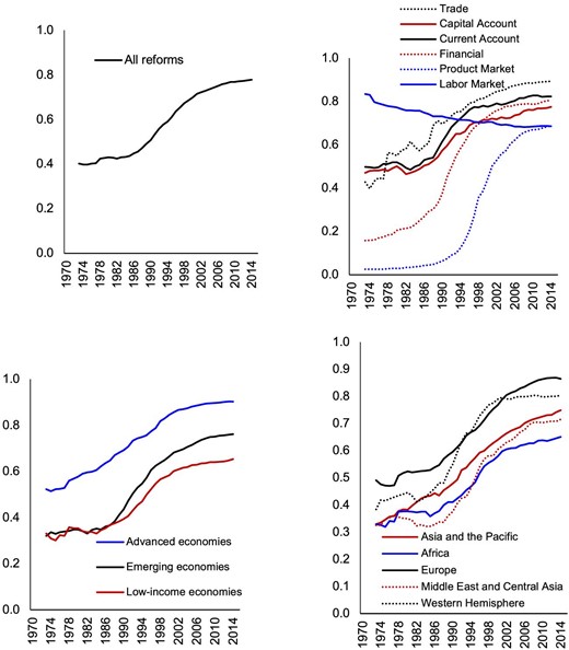
Stylized facts on structural reform. The indicators range from 0 (less liberalization) to 1 (more liberalization).
Second, the reform process has proceeded unevenly across sectors (top right): reforms are more prevalent in domestic finance, trade, capital, and current account than in product and labor markets. The major liberalizations in trade occurred in the 1970s and 1980s, in domestic and external finance in the early 1990s, and in the product market in the late 1990s. We find no reform trend for labor market regulation (EPL), and even some regulatory tightening in recent years.
The third pattern we observe is that advanced economies are more liberalized than emerging markets and low-income counties (bottom left). Furthermore, while emerging markets and low-income countries had a similar degree of regulation until the 1990s, reform liberalization has been stronger in emerging markets since then. Again, EPL is an exception: no systematic differences emerge across countries at different levels of development.
Fourth, liberalization has been the strongest in Europe, and more modest in the Middle East/Central Asia and sub-Saharan Africa (bottom right). Examples of major reform reversals include the capital and current accounts regulatory tightening in Argentina after the collapse of its currency board in the early 2000s; the significant increase in tariffs in Thailand in the late 1990s; the increase in domestic financial regulation in Ecuador in the mid-2000s; the reversal of the privatization of Jordan's electricity sector in 2011; and the tightening of labor market reforms in Portugal in the mid-1970s.
4.2 Reforms and the Electoral Cycle
Table 4 reports reform liberalization and reform reversal—the annual change in the reform indicator—during the incumbent leader's electoral term. Three patterns are evident from the SRD data. First, liberalizing reforms are nearly three times more common than tightening reforms in both election and non-election years (1,772 and 620, respectively, in the SRD).13 Second, liberalization reforms are less frequent in election years than in non-election years. The opposite is true for tightening reforms, the intensity of which is relatively large during election years compared to non-election years. Third, liberalizations are more frequent and larger in magnitude when economic conditions are weak. This might suggest that reforms are often imposed during a crisis when the timing is not politically optimal. By contrast, tightening reforms, while still rare, are more frequent when the economy is expanding.
Change in the reform indicator in the electoral cycle (normalized by one standard deviation).
| All | Weak economic conditions | Strong economic conditions | |
|---|---|---|---|
| Reform_ey | 0.410 | 0.432 | 0.381 |
| Reform_ey (+) | 0.491 | 0.503 | 0.474 |
| Reversal_ey (−) | −0.072 | −0.065 | −0.081 |
| Reform_term | 0.628 | 0.687 | 0.555 |
| Reform_term (+) | 0.680 | 0.729 | 0.620 |
| Reversal_term (−) | −0.043 | −0.037 | −0.049 |
Notes: Reform_ey and Reform_term denote reforms in the election year and in the rest of the incumbent leader's term, respectively. Reform (+) and Reversal (−) denote liberalization and tightening reforms, respectively. Weak and strong economic conditions are defined as in equation (2).
4.3 Reforms and the Economy
To trace the output dynamic following reforms, we follow Jordà’s (2005) local projection method, which several other studies have employed, including Auerbach and Gorodnichenko (2013), Ramey and Zubairy (2018), and Alesina et al. (2019). This procedure does not impose dynamic restrictions embedded in vector autoregression specifications and is particularly suited to estimating nonlinearities in the dynamic response. The first regression we estimate is
in which y is the log of output; |${\alpha }_i$| are country fixed effects, included to account for differences in countries’ average growth rates; |${\gamma }_t$| are time fixed effects, included to take into account global shocks such as shifts in oil prices or the global business cycle; |$\Delta $|R denotes the change in the regulation indicator—that is, a reform. Note that R, the regulation index, increases with the degree of liberalization, thus a liberalizing reform implies a positive value of |$\Delta {R}_{i,t}\ $|and a tightening is a negative value. X is a set of control variables, including two lags of the dependent variable, two lags of the change in the reform indicator, and country-specific time trends (to account for country-specific regulation patterns before the reform).14
A second specification allows the response of output to vary with business cycle conditions (a continuum of states between extreme recessions and booms) at the time of the reform:
with |$F( {{z}_{it}} ) = \exp^{ - \gamma {z}_{it}}/( {\exp^{ - \gamma {z}_{it}}} ),{\rm{\ }}\gamma > 0$|, where z is an indicator of the state of the economy normalized to have zero mean and a unit variance. The indicator of the state of the economy considered in the analysis is GDP growth.15 The weights assigned to each regime vary between 0 and 1 according to the weighting function|${\rm{\ }}F$|, so that F can be interpreted as the probability of being in a given state of the economy. The coefficients |$\beta _k^L$| and |$\beta _k^H$| capture the impact of reforms at horizon k in cases of extreme recessions (|$F( {{z}_{it}} ) \approx 1$| when z goes to minus infinity) or booms (|$1 - F( {{z}_{it}} ) \approx 1$| when z goes to plus infinity), respectively.16 Following Auerbach and Gorodnichenko (2012, 5), we choose |$\gamma = 1.5$| so that the economy spends about 20% of the time in a recessionary regime (defined as |$F( {{z}_{it}} ) > 0.8$|), which broadly matches business cycle patterns in advanced and emerging markets.17 Qit is the same set of control variables used in equation (1) but now includes F(zit) to control for the cyclical position at the time of reforms.
This approach is equivalent to the smooth transition autoregressive model developed by Granger and Teräsvirta (1993) but has two advantages over their approach. First, our method permits a direct test of whether the effect of reforms varies across different regimes such as recessions and expansions. Second, compared with estimating structural vector autoregressions for each regime, it allows the effect of reforms to change smoothly between recessions and expansions by considering a continuum of states to compute the impulse response functions, thus making the response more stable and precise.
Equations (1) and (2) are estimated for each k = 0,…,5. Impulse response functions are computed using the estimated coefficients|${\rm{\ }}{\beta }_k$|, and the confidence bands associated with the estimated impulse response functions are obtained using the estimated standard errors of the coefficients |${\beta }_k$|, based on robust standard errors clustered at the country level.
Figure 2 shows the estimated dynamic evolution of GDP following a major reform—identified as a 1-standard-deviation change in the aggregate reform indicator—over the 5-year period, together with the 90% confidence interval around the point estimate. Major deregulation episodes have been associated with a positive and statistically significant increase in output of about 1% that occurs 5 years after the reform.
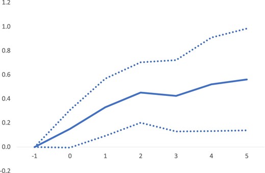
Macroeconomic effects of reform—output effect (%). Output effects estimated using equation (1). t = 0 is the year of the reform; solid lines denote the output resulting from a major reform event, defined as a 1-standard-deviation change in the reform indicator. Dotted lines denote 90% confidence bands.
An important concern is that reforms are likely to be endogenous to economic activity—that is, that reforms are correlated with the error term in equation (1)—which would prevent consistent estimates of the economic effect of reforms. We try to mitigate this issue by expanding the set of controls in equation (1) to include four observable variables that are related to both reforms and the error term.
First, we expand the set of controls to include income group fixed effects (advanced versus developing economies, measured at the beginning of the sample). This allows us to control for differential impacts of common shocks (including common reform waves) across countries at different stages of development. Second, since reforms are often part of stabilization packages designed to reduce public deficits and inflation, we include contemporaneous and lagged deficits and inflation as control variables. Third, to account for the possibility that reforms are implemented because of concerns regarding future weak economic growth, we follow Duval and Furceri (2018) and Furceri et al. (2019) by controlling for the expected values in t−1 of future GDP growth rates over periods t to t + k.18 Finally, we follow Ciminelli et al. (2022) and modify equation (1) to include forward reform variables (|$\mathop \sum \nolimits_{j = 1}^k \Delta {R}_{i,t + j}).$| This allows us to control for reforms that may occur during the impulse response function (IRF) horizon that the term |$\Delta {R}_{i,t}$| does not capture. As shown by Teulings and Zubanov (2014), not doing so would leave the model potentially mis-specified and bias our estimates. In our context, this is particularly important since reforms are sometimes either adopted in sequence or reversed after some years. The results presented in Online Appendix Figures A.1–A.4 are similar to, and not statistically different from, those obtained in the baseline.
We also directly tackle endogeneity by using the IV approach that we adopt for the election outcomes analysis; the instrument is based on improvements in the democracy scores of “neighboring” countries as in Giuliano et al. (2013) and Acemoglu et al. (2019). We consider alternative approaches to identifying neighbors based on trade and geographical proximity, common law origins, and military alliances. The results of these exercises are generally not satisfying; only one instrument (based on common legal origins) is relatively strong: the Kleibergen‒Paap rk Wald F statistic—equivalent to the F-effective statistic for non-homoskedastic error where there is one endogenous variable and one instrument (Andrews et al. 2019)—is higher than 10 but below the associated Stock–Yogo 10% critical value of 16.38. Figure A.5 reports the results obtained using the instrument. The increase in output following a major reform is slightly higher than that obtained using ordinary least squares (OLS), but the results should be treated with caution given the relative weakness of the instrument. Another consideration is that the instrument is unlikely to satisfy the exclusion restriction criteria since reforms in neighboring countries may directly affect domestic output through exports and imports. Indeed, when we control for net exports (or exports and imports separately) in the regression, the strength of the instrument significantly declines.
The dynamic evolution of output following reforms varies between liberalizing reforms and tightening reforms (Figure 3). The former are associated with a medium-term increase in output—with the effect being statistically significant only four years after the reform—while tightening reforms are associated with a contraction in output in the short term (the effect is less precisely estimated in the medium term). The difference in the absolute value of the effect between liberalizing and tightening reforms, however, is not statistically significant.
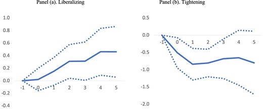
Macroeconomic effects of reform—output effect of liberalizing and tightening reforms (%). Output effects estimated using equation (1). t = 0 is the year of the reform; solid lines denote the output resulting from a major reform event, defined as a 1-standard-deviation change in the reform indicator. Dotted lines denote 90% confidence bands.
Prior work establishes that the change in output in response to reforms may mask different effects that vary with overall business conditions (Eggertsson et al. 2014; Cacciatore et al. 2016b; Duval and Furceri 2018; Furceri et al. 2018). In particular, we find that tightening reforms are associated with more limited short-term output losses when carried out in expansions than during recessions (Figure 4).19
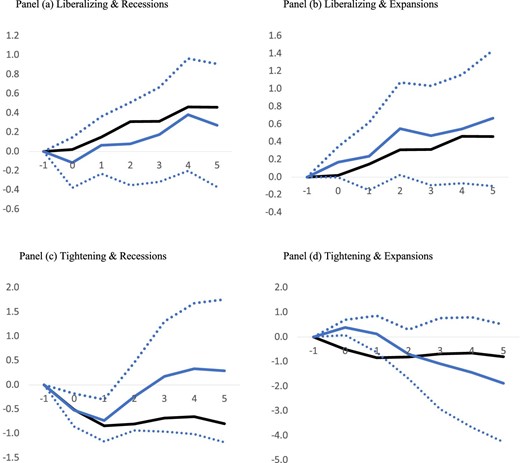
Macroeconomic effects of reform—output effect of liberalizing and tightening reforms depending on economic conditions (%). Output effects estimated using equation (1). t = 0 is the year of the reform; solid blue lines denote the output resulting from major reform tightening and liberalization events during recessions and expansions; solid black lines denote the unconditional response of output to major reform tightening and liberalization events shown in Figure 3; dotted lines denote 90% confidence bands.
We expand the analysis to examine whether the evolution of output varies across types of reforms. The results reported in Online Appendix Figure A.6 do not point to statistically significant differences between and among the types of reforms and their impact on growth, but the increase in output is larger and more precisely estimated for capital account reforms.
We also tested the possibility of complementarity (substitutability) between types of reforms using two alternative approaches. In the first, we expand equation (1) by including an interaction term between reforms in a given area h (|$\Delta R_{i,t}^h$|) and the average reform indicator in other areas (|$\Delta R_{i,t}^{ - h}$|), as well as these terms not interacted. In the second approach, we include an interaction term between a pair of reforms (|$\Delta R_{i,t}^{h1}$|*|$\Delta R_{i,t}^{h2}$|), as well as these terms not interacted. Online Appendix Figures A.7 and A.8 report the medium-term output effects for those combinations of reforms; the results are statistically significant and point to only two complementarities. First, labor market reforms are associated with larger output effects when reforms in other areas are also implemented (Online Appendix Figure A.7),20 especially in trade and capital accounts (Online Appendix Figure A.8). Second, trade (domestic finance) reforms are associated with stronger medium-term output gains when implemented together with domestic finance (trade) reforms.
Overall, this section presents some interesting, stylized facts about the association between reforms and economic outcomes, which are relevant to the electoral effects of reforms. First, it takes up to 4 years for outputs to increase following major liberalizing reforms. Tightening reforms, by contrast, are associated with a more immediate contraction of the economy. Second, tightening reforms tend to be associated with larger (smaller) output contractions during a downturn (upturn) in the business cycle.
5. Electoral Impact of Economic Reforms
5.1. Reforms and Elections
Our baseline specification is as follows:
where i denotes the country and t the election year. We examine changes in the reform index in the election year using Reform_eyi,t, which is the change in the unweighted average of all reform indicators in the election year. When elections take place in the first 3 months of the year, we code reforms as the change in the indicator in the previous year. We also examine Reform_term_resti,t, which is the change in the aggregate reform index during the rest of the incumbent coalition's term, plus the initial level of the reform indicator (Initial Regulationi,t−1) at the start of the term. In the benchmark specification, we control for three binary indicators (see Table 3): a developed-country dummy (1 = countries defined as advanced economies according to the IMF classification, and 0 otherwise), a dummy variable for new democracies (1 = countries for the first four elections after a year with a negative Polity score, and 0 otherwise), and a dummy variable for a majoritarian political system (1 = countries with an electoral system that awards seats in “winner-take-all” geographically based districts according to the Database of Political Institutions, and 0 otherwise) (Cruz, Keefer, and Scartascini 2016). To address potential endogeneity concerns resulting from the correlation between the timing of reforms and the business cycle, we control for GDP growth during the electoral year and during the rest of the incumbent's term.21 Finally, we use the incumbent's prior vote share in the election immediately preceding vote share (Incumbent Party Vote) to control for the government's popularity at the beginning of the term (Powell and Whitten 1993).22
A positive value of the reform indicator captures a move toward liberalization, while a negative value signals a move away from it. Thus, a positive coefficient on the reform variable implies an increase in the incumbent's vote share due to liberalization. All the results are scaled to denote the electoral effect of a major reform—identified as a change in the aggregate reform indicator equal to one standard deviation of the average change in the indicator. Equation (3) is estimated using OLS.
We begin by presenting the results in Table 5 with reforms during the election year (omitting reforms during the rest of the term) and find that election year reforms are associated with a statistically significant decrease in the vote share. A major reform (such as was implemented in Spain in 1986) is associated with a 1.4-percentage-point decrease in the vote share (column I).
The effect of reforms on electoral outcomes—election year.
| (I) | (II) | (III) | (IX) | (X) | |
|---|---|---|---|---|---|
| Reform_ey | −1.385*** | −1.594** | −1.748** | −1.361** | −1.391** |
| (0.457) | (0.632) | (0.661) | (0.639) | (0.641) | |
| Initial level regulation | −2.548 | 0.781 | 11.687 | 13.669 | −2.596 |
| (2.955) | (5.280) | (16.705) | (17.134) | (3.368) | |
| Growth_ey | 0.516** | 0.373 | 0.260 | 0.171 | |
| (0.206) | (0.267) | (0.410) | (0.429) | ||
| Growth_term | 0.411 | 0.692* | 0.834* | 0.748 | |
| (0.320) | (0.394) | (0.487) | (0.497) | ||
| Advanced economy | 3.409*** | 2.748** | |||
| (1.235) | (1.237) | ||||
| New democracies | 0.837 | 0.146 | 0.310 | −0.033 | 0.484 |
| (1.117) | (2.240) | (3.990) | (4.018) | (1.234) | |
| Majoritarian system | 2.314** | 4.763 | 10.350** | 11.147*** | 2.225** |
| (0.940) | (4.141) | (4.021) | (4.113) | (0.934) | |
| Lagged vote share | −0.146 | −0.242** | −0.265* | −0.265* | −0.136 |
| (0.093) | (0.103) | (0.137) | (0.135) | (0.088) | |
| Budget | 0.153 | ||||
| (0.267) | |||||
| Inflation | −0.006* | ||||
| (0.003) | |||||
| Country fixed effects | No | Yes | Yes | Yes | No |
| Country-specific time trends | No | No | Yes | Yes | No |
| R2 | 0.100 | 0.266 | 0.470 | 0.476 | 0.059 |
| Observations | 327 | 327 | 327 | 327 | 328 |
Notes: The dependent variable is the change in the incumbent party's vote share. Reform_ey denotes reforms in the election year. Estimates are based on equation (3). Standard deviations based on robust standard errors are in parentheses. *p < 0.1, **p < 0.05, ***p < 0.01.
Better economic conditions during either the election year or the incumbent's term are associated with more favorable political outcomes. In addition, we find that the changes in vote shares are typically larger in advanced economies and in majoritarian systems. The results are robust to including country fixed effects (column II), country-specific time trends (column III), and extending the set of controls to include changes in the budget balance and inflation during the electoral term (column IV). The magnitude of the effect of reforms on the vote share is almost identical to, albeit larger than, the one obtained in the baseline, although it is less precisely estimated.
In Table 6, we repeat the exercise for reforms implemented during the rest of the government's term—measured as the change in the indicator between the beginning of the term and the year prior to an election—omitting the election year reform indicator. There is no negative effect on the incumbent's vote share. The other coefficients remain stable relative to those in Table 5. When we introduce both reforms in the election year and in the rest of the term in the same model (Table 7), the election-year regressor maintains the same negative and highly statistically significant effect as in Table 5 and the “rest-of-the-term” regressor remains insignificant as in Table 6. Finally, these results are almost unchanged when we exclude GDP growth during the election year and the rest of the incumbent's term (Table 7, column V). This is consistent with the evidence presented in Section 4 that the economic effects of reforms take time to materialize and are often not observable until the next term of office (an incumbent leader's average tenure is about 3.5 years). The results also suggest that endogeneity due to the correlation between the timing of the reform and the business cycle does not obviously affect the estimates.
The effect of reforms on electoral outcomes—rest of term.
| (I) | (II) | (III) | (IV) | (V) | |
|---|---|---|---|---|---|
| Reform_term | −0.200 | −0.206 | 0.413 | −0.030 | −0.062 |
| (0.544) | (0.587) | (0.716) | (0.871) | (0.608) | |
| Initial level regulation | −0.548 | 2.922 | 16.310 | 14.677 | −0.282 |
| (3.105) | (5.021) | (17.715) | (18.675) | (3.415) | |
| Growth_ey | 0.468** | 0.299 | 0.167 | 0.081 | |
| (0.201) | (0.255) | (0.417) | (0.423) | ||
| Growth_term | 0.488 | 0.784* | 0.878* | 0.781 | |
| (0.327) | (0.406) | (0.484) | (0.506) | ||
| Advanced economy | 3.275** | 2.554** | |||
| (1.243) | (1.266) | ||||
| New democracies | 0.766 | 0.248 | 1.331 | 0.437 | 0.449 |
| (1.176) | (2.243) | (3.889) | (3.883) | (1.288) | |
| Majoritarian system | 2.303** | 4.396 | 10.057** | 10.067** | 2.209** |
| (0.992) | (3.977) | (4.430) | (4.810) | (0.978) | |
| Lagged vote share | −0.149 | −0.229** | −0.249* | −0.255* | −0.139 |
| (0.092) | (0.104) | (0.138) | (0.133) | (0.087) | |
| Budget | 0.163 | ||||
| (0.251) | |||||
| Inflation | 0.008*** | ||||
| (0.003) | |||||
| Country fixed effects | No | Yes | Yes | Yes | No |
| Country-specific time trends | No | No | Yes | Yes | No |
| R2 | 0.084 | 0.250 | 0.456 | 0.468 | 0.042 |
| Observations | 327 | 327 | 327 | 327 | 328 |
Notes: The dependent variable is the change in the incumbent party's vote share. Reform_ey denotes reforms in the election year. Estimates are based on equation (3). Standard deviations based on robust standard errors are in parentheses. *p < 0.1, **p < 0.05, ***p < 0.01.
The effect of reforms on electoral outcomes—election year versus rest of term.
| (I) | (II) | (III) | (IV) | (V) | |
|---|---|---|---|---|---|
| Reform_ey | −1.410*** | −1.615** | −1.730** | −1.362** | −1.409** |
| (0.473) | (0.647) | (0.664) | (0.640) | (0.646) | |
| Reform_term | −0.336 | −0.328 | 0.177 | −0.068 | −0.218 |
| (0.520) | (0.585) | (0.699) | (0.844) | (0.544) | |
| Initial level regulation | −3.399 | −0.491 | 13.450 | 13.017 | −3.157 |
| (3.005) | (5.188) | (17.792) | (18.302) | (3.288) | |
| Growth_ey | 0.512** | 0.362 | 0.260 | 0.171 | |
| (0.206) | (0.265) | (0.410) | (0.431) | ||
| Growth_term | 0.425 | 0.699* | 0.826* | 0.751 | |
| (0.323) | (0.398) | (0.486) | (0.495) | ||
| Advanced economy | 3.474*** | 2.782** | |||
| (1.245) | (1.253) | ||||
| New democracies | 0.804 | −0.036 | 0.380 | −0.063 | 0.461 |
| (1.109) | (2.187) | (3.950) | (3.981) | (1.231) | |
| Majoritarian system | 2.293** | 4.376 | 10.865** | 10.944** | 2.209** |
| (0.923) | (4.164) | (4.585) | (4.811) | (0.923) | |
| Lagged vote share | −0.146 | −0.243** | −0.264* | −0.265* | −0.136 |
| (0.093) | (0.103) | (0.137) | (0.134) | (0.088) | |
| Budget | 0.152 | ||||
| (0.266) | |||||
| Inflation | −0.006* | ||||
| (0.003) | |||||
| Country fixed effects | No | Yes | Yes | Yes | No |
| Country-specific time trends | No | No | Yes | Yes | No |
| R2 | 0.101 | 0.266 | 0.470 | 0.476 | 0.060 |
| Observations | 327 | 327 | 327 | 327 | 328 |
Notes: The dependent variable is the change in the incumbent party's vote share. Reform_ey and Reform_term denote reforms in the election year and in the rest of the incumbent leader's term, respectively. Estimates are based on equation (3). Standard deviations based on robust standard errors are in parentheses., *p < 0.1, **p < 0.05, ***p < 0.01.
5.2 Economic Conditions at the Time of Reform
We use the smooth transition function from equation (2) to allow the electoral effects of reforms to vary with business cycle conditions at the time of the reform in the election year and in the rest of the electoral term:
where i denotes the country and t the election year. As before, the coefficients, |$\beta _{1,2}^L$| and |$\beta _{1,2}^H$|, capture the electoral impact of a major reform in cases of extreme recessions (|$F( {{z}_{it}} ) \approx 1$| when z goes to minus infinity) and booms (|$1 - F( {{z}_{it}} ) \approx 1$| when z goes to plus infinity), respectively.
The results suggest a marked difference between the effects of reforms when the economy is strong versus weak in the election year and in the rest of the electoral term. The negative effect of reforms is concentrated solely among those enacted in election years with weak economic activity (Table 8). During periods of poor economic performance, a major reform—identified as a change in the aggregate reform indicator above one standard deviation of the average change in the indicator—is associated with a 2-percentage-point decline in the vote share. Note that we are still controlling for growth in the election year and in the rest of the electoral term.
The effect of reforms on electoral outcomes—recessions versus expansions.
| (I) | (II) | (III) | |
|---|---|---|---|
| Reform_ey (recessions) | −2.046** | −2.125** | |
| (0.782) | (0.799) | ||
| Reform_ey (expansions) | −0.601 | −0.669 | |
| (0.935) | (0.959) | ||
| Reform_term (recessions) | −0.005 | −0.791 | |
| (1.260) | (0.992) | ||
| Reform_term (expansions) | −0.386 | 0.075 | |
| (1.285) | (1.172) | ||
| Initial level regulation | −2.380 | −0.545 | −3.354 |
| (3.018) | (3.110) | (2.996) | |
| Growth_ey | 0.474** | 0.465** | 0.478** |
| (0.214) | (0.201) | (0.215) | |
| Growth_term | 0.415 | 0.503 | 0.391 |
| (0.321) | (0.365) | (0.352) | |
| Advanced economy | 3.341*** | 3.281** | 3.400*** |
| (1.227) | (1.249) | (1.229) | |
| New democracies | 0.821 | 0.785 | 0.746 |
| (1.124) | (1.156) | (1.107) | |
| Majoritarian system | 2.210** | 2.294** | 2.208** |
| (0.960) | (0.994) | (0.930) | |
| Lagged vote share | −0.144 | −0.149 | −0.144 |
| (0.094) | (0.092) | (0.094) | |
| Total effect recessions | −2.046 | −0.005 | −2.916 |
| Total effect expansions | −0.601 | −0.386 | −0.594 |
| F-test difference | 0.91 | 0.03 | 1.02 |
| R2 | 0.10 | 0.08 | 0.10 |
| Observations | 327 | 327 | 327 |
Notes: The dependent variable is the change in the incumbent party's vote share. Reform_ey and Reform_term denote reforms in the election year and in the rest of the incumbent leader's term, respectively. Estimates are based on equation (4). Standard deviations based on robust standard errors are in parentheses. *p < 0.1, **p < 0.05, ***p < 0.01.
In Table 9, we investigate whether liberalizing and tightening reforms produce different electoral effects if the policy change is a regulatory tightening or liberalization. Note that when the reform indicator has a negative value (tightening reforms), a positive coefficient implies that the reform leads to a loss of votes, and vice versa.23 The results in column I suggest that while liberalizing reforms have a negative and significant electoral cost when implemented during an election year, tightening reforms tend to increase the incumbent coalition's vote share, but not significantly. When we allow the effect of reforms to vary between good and bad economic times (column II), we continue to find that election year reforms during recessions decrease incumbent vote shares. A striking result is that incumbents are punished for reforms and reversals during the rest of their term when the reform change occurs in recession years. However, they are rewarded for reforms and reversals in non-election years when the reform change occurs during expansions—recall that we are still controlling for the rate of economic growth.24
The effect of reforms on electoral outcomes—reforms versus reversals.
| (I) | (II) | |
|---|---|---|
| Baseline | Recessions versus expansions | |
| Reform_ey (+) | −1.465** | |
| (0.579) | ||
| Reversal_ey (−) | 1.288 | |
| (1.513) | ||
| Reform_term (+) | −0.199 | |
| (0.531) | ||
| Reversal_term (−) | 1.123 | |
| (2.036) | ||
| Reform_ey (+) (recessions) | −2.098** | |
| (0.832) | ||
| Reversal_ey (−) (recessions) | 0.309 | |
| (1.345) | ||
| Reform_term (+) (recessions) | −2.329** | |
| (1.175) | ||
| Reversal_term (−) (recessions) | −6.322*** | |
| (1.936) | ||
| Reform_ey (+) (expansions) | −0.143 | |
| (0.997) | ||
| Reversal_ey (−) (expansions) | 3.643 | |
| (5.478) | ||
| Reform_term (+) (expansions) | 1.707* | |
| (0.923) | ||
| Reversal_term (−) (expansions) | 10.221*** | |
| (3.140) | ||
| F-test: Reform_ey (+) versus (−) | 0.01 | 14.84*** |
| Total effect recessions | −10.440 | |
| Total effect expansions | 15.428 | |
| F-test difference | 11.95*** | |
| R2 | 0.10 | 0.13 |
| Observations | 327 | 327 |
Notes: The dependent variable is the change in the incumbent party's vote share. Reform_ey and Reform_term denote reforms in the election year and in the rest of the incumbent leader's term, respectively. Reform (+) and Reversal (−) denote liberalization and tightening reforms, respectively. Estimates are based on equation (4). Additional controls in the baseline specifications are included but not reported. Standard deviations based on robust standard errors are in parentheses. *p < 0.1, **p < 0.05, ***p < 0.01.
5.3 Summing Up and Relation to Theoretical Work
We demonstrate the importance of the timing of a reform relative to both the electoral and business cycles. We find that the vote share of the main governing party (or coalition) declines when liberalizing reforms are implemented in an election year. This electoral cost disappears when reforms are implemented at the beginning of an incumbent's term, and thus have time to generate positive economic effects. This result may suggest that voters are short-sighted and/or do not appreciate how long it takes a reform to generate benefits (Bonfiglioli and Gancia 2013). Another interpretation, which is consistent with the theoretical literature on the concentration of losses to incumbents from reform, is that reforms generate concentrated economic losses, and the losers are inclined to retaliate by opposing reforming governments if a reform occurs close to an election. Retaliation for losses is itself a rational response in a repeated interaction between elected officials and different constituencies.
The state of the business cycle also influences how reforms shape electoral results. We show that when economies are in contraction, voters penalize both liberalizing and tightening reforms at the ballot box. Yet, they do not appear to punish (and sometimes even reward) incumbents for reforms undertaken during a growth expansion.
Voters therefore seem to be unable to accurately distinguish between the effects of the business cycle and those of the reform. They appear to attribute the state of the economy to recent reforms without allowing for delays in the transmission of reforms’ effects on the economy. This interpretation is consistent with the literature on the signal extraction problem facing voters (Ferejohn 1986; Wolfers 2002; Achen and Bartels 2016). According to this strand of research, voters struggle to determine how much of a downturn is due to the policymaker, how much is due to luck, and whether challengers will credibly commit to policies that enhance economic performance. In some ways, undertaking reforms, which can have a clear negative impact on those who benefited from the prior regulatory regime, pushes the signal extraction problem in the direction of blaming reformers.
6. Endogeneity
6.1 Endogeneity Issues
Many sources of potential endogeneity could bias our results, but two are particularly important: (i) reforms are often implemented as part of stabilization packages designed to reduce the budget deficit and inflation and (ii) the economic cycle might affect the timing of the reform. We show that the results are substantively unchanged when we control for macroeconomic policies and outcomes: see column IV in Tables 5–7, which include inflation and budget deficit terms; the reform coefficient estimates are largely unchanged. In column V in Tables 5–7, we omit the economic growth terms, and again the coefficient estimates are largely unchanged.
Another important potential source of endogeneity is the fact that governments can sometimes choose when to implement reforms.25 The popularity of the government, for example, can affect its choice of the timing and direction of the reform decision. To examine whether government popularity moderates the electoral effects of reforms, we first regress our reform variable against the level of government popularity at the beginning of the year of the reform as well as country fixed effects. To measure government popularity, we use the Index of popular support, a standardized variable based on public opinion polls provided by the International Country Risk Guide (ICRG) for over 130 countries since 2001 (see Herrera et al. 2020). The results establish that the index of popular support is positively and significantly associated with an increase in the reform index.26 Since popularity in an election year is closely related to the vote share at the time of election, not controlling for popularity might lead to a potential underestimate of the political costs of reforms.27
In Table 10, we estimate a baseline model (cf. Table 7.I), and two models including government popularity as a regressor. The data availability for government popularity shrinks the sample by nearly 50% (327 observations versus 164). The coefficient estimates on reform in an election year change little (−1.41*** versus −1.31**) despite the sample shrinkage (Table 10.I). Government popularity, when added to the model (10.II), has a positive and highly statistically significant coefficient estimate, and the estimated coefficient of reform in an election year increases by nearly 40% and is estimated more precisely (−1.81***). Government popularity thus appears to affect the estimated effect of election reforms on incumbent vote shares.
The effect of reforms on electoral outcomes—election year versus rest of term controlling for government popularity.
| (I) | (II) | (III) | |||
|---|---|---|---|---|---|
| Reform_ey | −1.311** | −1.810*** | |||
| (0.626) | (0.625) | ||||
| Reform_term | −0.169 | −0.511 | −0.596 | ||
| (0.978) | (0.912) | (0.875) | |||
| Reform_ey-Low popular support | −1.953** | ||||
| (0.794) | |||||
| Reform_ey_High popular support | −1.156 | ||||
| (1.132) | |||||
| Initial level regulation | 3.614 | −2.122 | −2.316 | ||
| (6.279) | (6.373) | (6.352) | |||
| Growth_ey | 0.462** | 0.336 | 0.334 | ||
| (0.234) | (0.219) | (0.219) | |||
| Growth_term | 0.480 | 0.161 | 0.168 | ||
| (0.340) | (0.331) | (0.333) | |||
| Advanced economy | 1.527 | 2.427 | 2.409 | ||
| (1.602) | (1.645) | (1.640) | |||
| New democracies | 0.403 | 1.396 | 1.470 | ||
| (1.562) | (1.602) | (1.573) | |||
| Majoritarian system | 0.355 | 0.678 | 0.709 | ||
| (1.211) | (1.141) | (1.134) | |||
| Lagged vote share | −0.229** | −0.231*** | −0.231*** | ||
| (0.092) | (0.085) | (0.085) | |||
| Popular support | 5.826*** | 5.536*** | |||
| (1.287) | (1.476) | ||||
| R2 | 0.11 | 0.17 | 0.17 | ||
| Observations | 164 | 164 | 164 |
Notes: The dependent variable is the change in the incumbent party's vote share. Standard deviations based on robust standard errors in are parentheses. Reform_ey and Reform_term denote reforms in the election year and in the rest of the incumbent leader's term, respectively. Estimates in column I are based on equation (3). Estimates in column II are based on equation (3) with the addition of political support as a control variable. Estimates in column III are based on the following equation: |$\Delta \textit{Incumbent}\ \textit{Vote}\ \textit{Share}_{i,t} = {\beta }_0 + \beta _1^A\ D*\textit{Reform}_{e{y}_{i,t}} + \beta _2^A\ D*\textit{Reform}_{ter{m}_{i,t}} + \beta _1^C\ ( {1 - D} )* \textit{Reform}_{e{y}_{i,t}} \\ + \beta _2^{}\textit{Reform}_{ter{m}_{i,t}} + {\beta }_3\textit{Growth}_{e{y}_{i,t}} + {\beta }_4\textit{Growth}_{ter{m}_{i,t}} + {\beta }_4\textit{Developed}\ \textit{Country}_i + {\beta }_5\textit{NewDemocracy}_{i,t} + {\beta }_6\textit{Majoritarian}\ \textit{system}_{i,t} + {\beta }_7\textit{Initial}\ \textit{Regulation}_{i,t - 1} + {\beta }_8\textit{Incumbent}\ \textit{Vote}\ \textit{Share}_{i,t - 1} + {\beta }_9{\textit{Political}}\ {\textit{support}}_{i,t} + \ {\varepsilon }_{i,t}$| where |${\textit{Political}}\ \textit{support}$| is the ICRG indicator in the election year, and D is a dummy variable that equals 1 when political support is above average and 0 otherwise. *p < 0.1, **p < 0.05, ***p < 0.01.
In Table 10.III, we partition reform election year effects by the popularity of governments. Less popular governments might suffer greater electoral losses from election year reforms than more popular governments, although the difference between the coefficient estimates is not statistically significant.
Another important endogeneity issue relates to the timing of elections. In some countries, elections may be called early, while exogenous elections correspond to about 40% (127 out of 327) of the elections in our sample. It is also possible that an election's timing could be correlated with economic conditions or the incumbent's popularity, which would bias our estimates. We address this issue by focusing on countries/time periods with exogenous elections—that is, those for which the head of government does not have the power to dissolve parliament and call new elections.
Next, we evaluate reforms that are externally mandated and not solely the choice of a national government. Clearly, a country entering into an IMF-supported program is endogenous and such programs are often associated with policies to reduce domestic imbalances, which can have direct electoral implications (Dreher 2004; Rickard and Caraway 2014; Kosmidis 2018).28 To address this issue, equation (3) controls for a dummy that takes a value of 1 during an IMF program, and 0 otherwise, and for the change in the budget balance and inflation during the electoral term. Finally, this approach assumes that reforms implemented outside an IMF program do not have political costs. As a result, this identification strategy could introduce an “attenuation” bias and underestimate the impact of IMF-mandated reforms on the vote share.
Finally, we use an IV proposed by Giuliano et al. (2013) and applied in a different context by Acemoglu et al. (2019) to how democracy affects economic growth.29 The instrument is the weighted average of the change in the democracy indicator in trading partners over the last 2 years; the weights are determined by the strength of trade linkages with other countries.30 The first-stage estimates suggest that this instrument is “strong” and statistically significant. The Kleibergen‒Paap rk Wald F statistic—which is equivalent to the F-effective statistic for non-homoscedastic error if there is one endogenous variable and one instrument (Andrews et al. 2019)—is higher than the associated Stock–Yogo critical value (see also Table A.3, Online Appendix A).
In addition, we believe the instrument to be plausibly exogenous, since changes in democratic institutions in trading-partner countries are unlikely to affect re-election—that is, be correlated with the error term of equation (3)—once we control for domestic economic growth in the electoral term and therefore potential effects on electoral outcomes through this channel.31 We provide several tests to support this claim.
First, we regress the residuals from equation (3) against the instrument. The results of this exercise suggest that the instrument is not statistically significantly correlated with the residuals.32 Second, following Bonfiglioli et al. (2022), we expand the set of controls in equation (3) to include four spillover variables that capture the potential effects of economic characteristics in trading partners that may affect electoral outcomes and be correlated with our instrument: (i) reform progress, (ii) real per capita GDP, (iii) inflation, and (iv) interest rates (namely, the 10-year government bond rates). The resulting second-stage estimates (Table A.4) are extremely close to those obtained in Table 10. Following Bonfiglioli et al. (2022), we also consider the possibility that countries experiencing comparable changes in certain observable characteristics may be hit by similar unobservable shocks that influence the electoral outcomes. In particular, we divide countries into four bins corresponding to the quartile of certain characteristics (reform progress, GDP growth, inflation, and budget deficit) during the election year and interact a dummy for each bin with year dummies. Adding these interactions to the baseline specification does not alter our findings (Online Appendix Table A.5).33 Finally, we analyze how violations of the exclusion restrictions would affect our key parameter of interest, |${\beta }_1$|. Using the approach proposed by Conley et al. (2012) and developed by Bonfiglioli et al. (2022), we estimate the following specification using the IV approach:
where the parameter |$\mu $| denotes the extent to which the exclusion restriction is violated, and |$\mu = 0$| represents the case in which the exclusion restriction is satisfied. We estimate equation (5) for different values of |$\mu $| and compare the resulting inference of |${\beta }_1$|. We set the parameter |$\mu $| as a function of parameter |$\delta $|, which we progressively raise to generate increasingly stronger violations of the exclusion restriction: |$\mu = - 3.836*\delta /3$|, where |$- 3.836$| is our baseline IV estimate of |${\beta }_1$| and 3 is the ratio of the standard deviation of our instrument to the standard deviation of |$Refor{m}_{e{y}_{i,t}}$|. |$\delta > 0$| corresponds to a violation of the exclusion restriction such that the direct electoral effect of one standard deviation increase in the instrument has the same effect of |$\delta $| standard deviations increase in our reform indicator. Online Appendix Table A.6 presents the IV estimates for at various values of |$\delta $|. The estimates remain statistically significant for |$\delta $| up to 0.85 and become statistically insignificant at |$\delta = 1$|. In other words, for our parameter of interest to become statistically insignificant, and thus uninformative about the causal impact of reforms on election, the direct effect of our instrument on electoral outcomes would have to be almost as much as the effect of domestic reforms, which is highly implausible.
6.2 Results Addressing Endogeneity
Tables 11–13 report our results addressing endogeneity. The patterns of the OLS regression results reported in Tables 5–9 are confirmed in these three specifications. Table 11 shows that the estimated effects of reforms on vote shares in where the timing of elections is exogenously fixed (11.III), or limited to the case of IMF-imposed reforms (11.IV), or using the IV approach (11.V), are much larger than those obtained with OLS (column I, which repeats the OLS results in column I of Table 7) and fixed effects (column II) in Table 11. This finding confirms that politicians may decide not to implement reforms because they are aware of the possible political costs—which in our framework implies a downward bias in the OLS coefficient estimates. The coefficients on the other control variables remain stable.
The effect of reforms on electoral outcomes—exogeneity checks.
| (I) | (II) | (III) | (IV) | (V) | |
|---|---|---|---|---|---|
| OLS | OLS w/FE | Ex. elections | IMF | IV | |
| Reform_ey | −1.410*** | −1.615*** | −1.983*** | −2.554** | −3.836*** |
| (0.473) | (0.585) | (0.522) | (1.071) | (0.792) | |
| Reform_term | −0.336 | −0.328 | −0.298 | −0.624 | −0.570 |
| (0.520) | (0.529) | (1.048) | (1.224) | (0.523) | |
| Initial level regulation | −3.399 | −0.491 | −2.200 | −0.741 | −8.305** |
| (3.005) | (4.691) | (7.307) | (2.977) | (3.743) | |
| Growth_ey | 0.512** | 0.362 | 0.502* | 0.502** | 0.586*** |
| (0.206) | (0.240) | (0.269) | (0.208) | (0.222) | |
| Growth_term | 0.425 | 0.699* | 1.191** | 0.445 | 0.316 |
| (0.323) | (0.360) | (0.568) | (0.313) | (0.341) | |
| Advanced economy | 3.474*** | 4.948 | 2.776** | 3.815*** | |
| (1.245) | (2.985) | (1.321) | (1.281) | ||
| New democracies | 0.804 | −0.036 | 1.713 | 1.114 | 0.870 |
| (1.109) | (1.977) | (2.253) | (1.127) | (1.039) | |
| Majoritarian system | 2.293** | 4.376 | 0.536 | 2.131** | 2.275*** |
| (0.923) | (3.765) | (2.480) | (0.999) | (0.856) | |
| Lagged vote share | −0.146 | −0.243** | −0.009 | −0.135 | −0.141 |
| (0.093) | (0.094) | (0.121) | (0.094) | (0.093) | |
| Kleibergen–Paap rk Wald F statistic | 25.92 | ||||
| Stock–Yogo 10% critical value | 16.38 | ||||
| (Uncentered) R2 | 0.10 | 0.10 | 0.14 | 0.09 | 0.23 |
| Observations | 327 | 327 | 127 | 327 | 327 |
Notes: The dependent variable is the change in the incumbent party's vote share. Reform_ey and Reform_term denote reforms in the election year and in the rest of the incumbent leader's term, respectively. Estimates are based on equation (3). Standard deviations based on robust standard errors are in parentheses. *p < 0.1, **p < 0.05, ***p < 0.01.
The effect of reforms on electoral outcomes—recessions versus expansions, exogeneity checks.
| (I) | (II) | (III) | (IV) | (V) | |
|---|---|---|---|---|---|
| OLS | OLS w/FE | Ex. elections | IMF | IV | |
| Reform_ey (recessions) | −2.125** | −1.923* | −2.681*** | −0.943 | −3.679*** |
| (0.799) | (1.003) | (0.407) | (5.907) | (0.597) | |
| Reform_ey (expansions) | −0.669 | −0.993 | −0.720 | −3.447 | −0.046 |
| (0.959) | (1.104) | (2.100) | (2.405) | (0.845) | |
| Reform_term (recessions) | −0.791 | 0.965 | −1.233 | −1.146 | −1.096 |
| (0.992) | (1.395) | (1.712) | (1.834) | (0.977) | |
| Reform_term (expansions) | 0.075 | −1.479 | 0.521 | −0.237 | 0.237 |
| (1.172) | (1.415) | (2.265) | (2.676) | (1.135) | |
| Initial level regulation | −3.354 | 0.235 | −2.001 | −0.789 | −4.263 |
| (2.996) | (4.595) | (7.412) | (2.987) | (3.031) | |
| Growth_ey | 0.478** | 0.319 | 0.451 | 0.510** | 0.436* |
| (0.215) | (0.239) | (0.295) | (0.208) | (0.225) | |
| Growth_term | 0.391 | 0.833** | 1.145* | 0.428 | 0.354 |
| (0.352) | (0.415) | (0.572) | (0.311) | (0.353) | |
| Advanced economy | 3.400*** | 4.899 | 2.744** | 3.370*** | |
| (1.229) | (2.981) | (1.327) | (1.209) | ||
| New democracies | 0.746 | 0.157 | 1.519 | 1.090 | 0.712 |
| (1.107) | (1.901) | (2.433) | (1.143) | (1.074) | |
| Majoritarian system | 2.208** | 4.746 | 0.595 | 2.135** | 2.057** |
| (0.930) | (3.743) | (2.459) | (0.994) | (0.912) | |
| Lagged vote share | −0.144 | −0.244** | −0.002 | −0.137 | −0.139 |
| (0.094) | (0.093) | (0.123) | (0.094) | (0.091) | |
| Total effect recessions | −2.916 | −0.958 | −3.914 | −2.089 | −4.775 |
| Total effect expansions | −0.594 | −2.472 | −0.199 | −3.684 | 0.191 |
| F-test difference | 1.02 | 0.23 | 0.96 | 0.03 | 4.51** |
| Kleibergen–Paap rk Wald F statistic | 184.4 | ||||
| Stock–Yogo 10% critical value | 16.38 | ||||
| (Uncentered) R2 | 0.10 | 0.10 | 0.14 | 0.09 | 0.26 |
| Observations | 327 | 327 | 127 | 327 | 327 |
Notes: The dependent variable is the change in the incumbent party's vote share. Reform_ey and Reform_term denote reforms in the election year and in the rest of the incumbent leader's term, respectively. Estimates are based on equation (4). Standard deviations based on robust standard errors are in parentheses. *p < 0.1, **p < 0.05, ***p < 0.01.
The effect of reforms on electoral outcomes—reforms versus reversals with exogeneity checks.
| (I) | (II) | (III) | (IV) | |
|---|---|---|---|---|
| OLS | OLS w/FE | Ex. elections | IV | |
| Reform_ey (+) (recessions) | −2.098** | −1.367 | −2.810*** | −3.311*** |
| (0.832) | (1.007) | (0.940) | (0.595) | |
| Reversal_ey (−) (recessions) | 0.309 | 3.096 | 0.839 | −0.194 |
| (1.345) | (1.987) | (1.978) | (1.429) | |
| Reform_term (+) (recessions) | −2.329* | −0.513 | −2.350 | −2.430** |
| (1.175) | (1.535) | (2.947) | (1.117) | |
| Reversal_term (−) (recessions) | −6.322*** | −9.731*** | −2.837 | −5.481*** |
| (1.936) | (2.326) | (3.417) | (1.492) | |
| Reform_ey (+) (expansions) | −0.143 | −0.436 | 0.850 | 0.292 |
| (0.997) | (1.203) | (2.413) | (0.828) | |
| Reversal_ey (−) (expansions) | 3.643 | 4.307 | 6.840 | 3.967 |
| (5.478) | (5.703) | (9.496) | (5.261) | |
| Reform_term (+) (expansions) | 1.707* | 0.566 | 2.765 | 1.730** |
| (0.923) | (1.218) | (1.915) | (0.882) | |
| Reversal_term (−) (expansions) | 10.221*** | 15.001*** | 8.671*** | 9.856*** |
| (3.140) | (2.889) | (3.079) | (2.875) | |
| Initial level regulation | −3.049 | 0.963 | −0.880 | −3.859 |
| (3.247) | (4.759) | (7.333) | (3.262) | |
| Growth_ey | 0.457* | 0.372 | 0.299 | 0.377 |
| (0.246) | (0.315) | (0.354) | (0.234) | |
| Growth_term | 0.091 | 0.369 | 0.869 | 0.078 |
| (0.365) | (0.466) | (0.751) | (0.354) | |
| Advanced economy | 3.466*** | 5.237* | 3.417*** | |
| (1.287) | (2.881) | (1.248) | ||
| New democracies | 1.310 | 1.198 | 2.427 | 1.285 |
| (1.109) | (1.971) | (2.492) | (1.081) | |
| Majoritarian system | 2.175** | 3.076 | 0.774 | 2.034** |
| (0.963) | (4.371) | (2.392) | (0.937) | |
| Lagged vote share | −0.160* | −0.263*** | −0.031 | −0.154* |
| (0.093) | (0.093) | (0.129) | (0.089) | |
| Total effect recessions | −10.440 | −8.515 | −7.158 | −11.416 |
| Total effect expansions | 15.428 | 19.438 | 19.126 | 15.845 |
| F-test: difference | 11.95*** | 9.71*** | 4.77** | 14.18*** |
| Kleibergen–Paap rk Wald F statistic | 293.32 | |||
| Stock–Yogo 10% critical value | 16.38 | |||
| (Uncentered) R2 | 0.13 | 0.14 | 0.18 | 0.29 |
| Observations | 327 | 327 | 127 | 327 |
Notes: The dependent variable is the change in the incumbent party's vote share. Reform_ey and Reform_term denote reforms in the election year and in the rest of the incumbent leader's term, respectively. Reform (+) and Reversal (−) denote liberalization and tightening reforms. Estimates based on equation (4). Standard deviations based on robust standard errors are in parentheses. *p < 0.1, **p < 0.05, ***p < 0.01.
Table 12 adds the business cycle variables and otherwise repeats the OLS (I), OLS with country fixed effects (II), exogenous elections (III), IMF reforms (IV), and IV method (V) pattern. The results regarding the electoral cost of election year reforms occurring mostly when the election year is in a recession are confirmed. The distinction between reforms implemented in recessions and in expansions is not precisely estimated for IMF-imposed reforms, however. The reason is that most IMF-imposed reforms occur during recessions—that is, countries are more likely to request IMF support when they are in a difficult economic situation (see Online Appendix Table A.1).
Table 9 (II) establishes that incumbents are punished for reforms and reversals during the rest of their term when reforms occur in recession years. Incumbents, in contrast, tend to be rewarded for reforms and reversals in non-election years when these occur in expansions. Table 13 confirms these results when distinguishing between liberalizing and tightening reforms and their timing relative to the business cycle.34
7. Extensions
7.1 Extended Empirical Framework
In this section, we explore several extensions. We examine whether the effect of reforms on electoral outcomes varies: (i) across types of reforms, (ii) between coalition and single-party governments, (iii) between advanced and developing economies, (iv) between majoritarian and proportional systems, and (v) between old and new democracies. The cases (ii)–(v) are tested by extending the baseline specification as follows:
where D is a dummy variable as described below for each analysis. Equation (6) is also estimated using OLS for the three strategies we use to mitigate endogeneity concerns. We further extend equation (5) to examine the electoral effect of reforms for cases (i)–(v) during periods of recession and expansions.35
7.2 Results
7.2.1 Types of Reforms
We estimate equation (3) to differentiate the effect of financial sector reforms (Domestic Finance, Capital, and Financial Current) from other domestic sector reforms (Trade, Product, and Labor markets).36 The results show that, while the effect of financial sector reforms on the vote share is large and statistically significant, the effect of real sector reform is not statistically significantly different from zero (Table 14). Similar results are obtained when estimating each reform separately (Online Appendix Table A.8). Online Appendix Table A.9 extends the financial versus real sector analysis to reversals and liberalizations, and demonstrates that only financial reforms enacted in election years harm incumbents’ electoral prospects. One potential explanation for this result is that financial sector reforms may be especially prone to engender increased income inequality (see, e.g. de Han and Sturm 2017; Furceri and Loungani 2018; Furceri et al. 2019; Ostry et al. 2021).37 In addition, we find some evidence that in bad times, financial reforms are associated with lower incumbent vote shares (Online Appendix Table A.10). Yet in good times, real sector reforms tend to have a positive effect, but the coefficients are rarely statistically significant.38 In other words, real sector reforms enacted in good times may help governments get re-elected. Overall, these results are consistent with voters being unable to distinguish between the expected long-run growth effects of financial sector reforms and the performance of the economy due to the underlying economic conditions at the time of the reform.
The effect of reforms on electoral outcomes—financial versus real reforms.
| (I) | (II) | (III) | (IV) | (V) | (VI) | (VII) | (VIII) | (IX) | (X) | |
|---|---|---|---|---|---|---|---|---|---|---|
| OLS | OLS w/FE | Exogenous elections | IMF | IV | ||||||
| Finance | Real | Finance | Real | Finance | Real | Finance | Real | Finance | Real | |
| Reform_ey | −3.673*** | 0.856 | −4.110** | 0.327 | −4.545*** | 3.888 | −10.306*** | 5.993 | −8.343*** | 0.148 |
| (1.181) | (1.077) | (1.584) | (1.191) | (1.245) | (3.645) | (3.371) | (7.344) | (1.875) | (8.310) | |
| Reform_term | 0.009 | −0.628 | −0.068 | −0.674 | 2.214 | −1.063 | −0.943 | −5.992* | −0.277 | −0.587 |
| (1.278) | (0.893) | (1.315) | (0.928) | (1.925) | (2.048) | (1.899) | (3.060) | (1.232) | (0.997) | |
| Initial level regulation | −1.525 | −0.353 | 0.108 | 2.380 | 2.293 | 1.114 | −0.777 | −0.394 | −3.827 | −0.686 |
| (2.461) | (3.113) | (3.628) | (4.161) | (4.451) | (7.397) | (2.184) | (3.075) | (2.638) | (5.092) | |
| Growth_ey | 0.287 | 0.467** | 0.258 | 0.298 | 0.442* | 0.414 | 0.319 | 0.493** | 0.299 | 0.473** |
| (0.256) | (0.199) | (0.286) | (0.233) | (0.258) | (0.249) | (0.253) | (0.200) | (0.262) | (0.205) | |
| Growth_term | 0.673** | 0.484 | 0.880*** | 0.774** | 0.987** | 1.343** | 0.679** | 0.419 | 0.609* | 0.483 |
| (0.311) | (0.326) | (0.324) | (0.370) | (0.454) | (0.528) | (0.314) | (0.318) | (0.314) | (0.324) | |
| Advanced economy | 3.298*** | 3.189*** | 4.124* | 5.290* | 2.519** | 2.603** | 3.698*** | 3.211*** | ||
| (1.217) | (1.173) | (2.232) | (2.826) | (1.237) | (1.153) | (1.230) | (1.108) | |||
| New democracies | 0.739 | 0.668 | 0.126 | 0.020 | 1.188 | 1.385 | 1.163 | 1.022 | 0.742 | 0.708 |
| (1.125) | (1.162) | (1.966) | (1.930) | (1.917) | (2.507) | (1.137) | (1.184) | (1.086) | (1.112) | |
| Majoritarian system | 1.536 | 2.264** | 4.656 | 3.855 | 0.252 | 0.409 | 1.293 | 1.926* | 1.528 | 2.280** |
| (1.042) | (1.015) | (3.513) | (3.728) | (2.158) | (2.797) | (1.030) | (1.006) | (1.062) | (0.981) | |
| Lagged vote share | −0.182** | −0.150 | 0.245*** | 0.228** | −0.027 | −0.019 | −0.176** | −0.158* | −0.177** | −0.149* |
| (0.082) | (0.091) | (0.079) | (0.096) | (0.112) | (0.113) | (0.081) | (0.085) | (0.081) | (0.090) | |
| Kleibergen–Paap rk Wald F statistic | 31.37 | 9.03 | ||||||||
| Stock–Yogo 10% critical value | 16.38 | 16.38 | ||||||||
| (Uncentered) R2 | 0.11 | 0.09 | 0.11 | 0.08 | 0.15 | 0.12 | 0.11 | 0.1 | 0.08 | 0.08 |
| Observations | 363 | 327 | 363 | 327 | 140 | 127 | 363 | 327 | 363 | 327 |
Notes: The dependent variable is the change in the incumbent party's vote share. Reform_ey and Reform_term denote reforms in the election year and in the rest of the incumbent leader's term, respectively. Estimates based on equation (3). Standard deviations based on robust standard errors are in parentheses. *p < 0.1, **p < 0.05, ***p < 0.01.
7.2.2 Coalition versus Single-Party Government
We expect the electoral penalty for reforms to fall largely on either the party governing alone or the majority party in a coalition. To test this prediction, we estimate a specification analogous to equation (6), in which D is a dummy variable that takes a value of 1 when the government is governing alone, and 0 otherwise. The results suggest that the effect of reforms on the incumbent majority party's vote share is three times larger when the party is governing alone than when it governs in a coalition (Table 15 (I)), particularly during recessions (Online Appendix Table A.11 (I)).39 This is consistent with prior findings in the literature on the clarity of responsibility (Powel and Whitten 1993).
The effect of reforms on electoral outcomes—governing alone versus coalition.
| (I) | (II) | (III) | (IV) | (V) | |
|---|---|---|---|---|---|
| OLS | OLS w/FE | Ex. elections | IMF | IV | |
| Reform_ey (Gov. alone) | −1.566*** | −1.902*** | −1.028*** | −1.568*** | −1.844*** |
| (0.517) | (0.677) | (0.254) | (0.556) | (0.385) | |
| Reform_term (Gov. alone) | −0.056 | −0.142 | −0.186 | 0.062 | −0.120 |
| (0.701) | (0.802) | (0.511) | (0.523) | (0.335) | |
| Reform_ey (Gov. in coalition) | −0.501 | −0.362 | 1.269 | 2.332 | −0.426 |
| (0.612) | (0.722) | (4.588) | (1.960) | (0.322) | |
| Reform_term (Gov. in coalition) | −0.862 | −0.782 | 0.991 | −9.081*** | −0.626 |
| (0.740) | (0.591) | (3.894) | (2.718) | (0.387) | |
| Initial level regulation | −3.307 | −0.591 | −2.224 | −0.139 | −7.224** |
| (2.970) | (4.594) | (7.411) | (2.937) | (3.483) | |
| Growth_ey | 0.514** | 0.379 | 0.490* | 0.613*** | 0.573*** |
| (0.205) | (0.246) | (0.267) | (0.194) | (0.218) | |
| Growth_term | 0.437 | 0.716** | 1.214** | 0.446 | 0.359 |
| (0.318) | (0.354) | (0.564) | (0.296) | (0.319) | |
| Advanced economy | 3.509*** | 5.136 | 3.020** | 3.716*** | |
| (1.241) | (3.105) | (1.296) | (1.264) | ||
| New democracies | 0.729 | −0.042 | 1.766 | 0.993 | 0.814 |
| (1.143) | (1.982) | (2.243) | (1.096) | (1.057) | |
| Majoritarian system | 2.248** | 4.446 | 0.209 | 1.901* | 2.344*** |
| (0.961) | (3.609) | (2.470) | (1.004) | (0.889) | |
| Lagged vote share | −0.146 | −0.248** | −0.015 | −0.110 | −0.141 |
| (0.093) | (0.094) | (0.118) | (0.092) | (0.093) | |
| Total effect (Gov. alone) | −1.622 | −2.044 | −1.214 | −1.506 | −1.964 |
| Total effect (Gov. in coalition) | −1.363 | −1.144 | 2.260 | −6.749 | −1.052 |
| F-test: difference | 0.06 | 0.43 | 0.17 | 8.07*** | 3.00* |
| Kleibergen–Paap rk Wald F statistic | 25.85 | ||||
| Stock–Yogo 10% critical value | 16.38 | ||||
| (Uncentered) R2 | 0.10 | 0.10 | 0.15 | 0.13 | 0.07 |
| Observations | 327 | 327 | 128 | 327 | 327 |
Notes: The dependent variable is the change in the incumbent party's vote share. Reform_ey and Reform_term denote reforms in the election year and in the rest of the incumbent leader's term, respectively. Estimates based on equation (6). Standard deviations based on robust standard errors are in parentheses. *p < 0.1, **p < 0.05, ***p < 0.01.
7.2.3 Advanced versus Developing Economies
To test whether the effect of reforms varies across countries, we estimate a specification analogous to equation (5), in which D is a dummy variable that takes a value of 1 for countries defined as advanced according to the IMF classification and 0 otherwise (Table 3). The results presented in Table 16 suggest that the effect is larger and more precisely estimated in developing than in advanced economies.40 This difference, however, is statistically significant for only two of the four specifications (II and IV—OLS fixed effects and IV). Table 16 does not include the IMF-imposed reforms specification since advanced countries have very few IMF programs.41
The effect of reforms on electoral outcomes—advanced versus developing economies.
| (I) | (II) | (III) | (IV) | |
|---|---|---|---|---|
| OLS | OLS w/FE | Ex. elections | IV | |
| Reform_ey (Adv.) | −0.655* | −0.373 | −4.495 | −0.751** |
| (0.348) | (0.405) | (3.518) | (0.343) | |
| Reform_ey (Dev.) | −2.038*** | −3.056*** | −1.855*** | −3.825*** |
| (0.672) | (0.727) | (0.557) | (0.782) | |
| Reform_term (Adv.) | −0.395 | −0.377 | 0.393 | −0.529 |
| (0.515) | (0.497) | (2.712) | (0.524) | |
| Reform_term (Dev.) | −0.350 | −0.351 | −0.361 | −0.505 |
| (0.912) | (1.018) | (1.057) | (0.859) | |
| Initial level regulation | −3.418 | −0.566 | −2.127 | −5.496 |
| (3.042) | (4.660) | (7.841) | (3.408) | |
| Growth_ey | 0.511** | 0.388 | 0.510* | 0.541** |
| (0.206) | (0.246) | (0.273) | (0.217) | |
| Growth_term | 0.406 | 0.646* | 1.217** | 0.339 |
| (0.322) | (0.345) | (0.578) | (0.323) | |
| Advanced economy | 2.944** | 4.940 | 2.398* | |
| (1.455) | (3.651) | (1.397) | ||
| New democracies | 0.816 | 0.211 | 1.795 | 0.866 |
| (1.126) | (2.050) | (2.203) | (1.071) | |
| Majoritarian system | 2.253** | 3.534 | 0.430 | 2.193** |
| (0.962) | (4.050) | (2.532) | (0.956) | |
| Lagged vote share | −0.144 | −0.253*** | −0.007 | −0.139 |
| (0.093) | (0.095) | (0.122) | (0.093) | |
| Total effect (Adv.) | −1.050 | −0.75 | −4.102 | −1.280 |
| Total effect (Dev.) | −2.388 | −3.407 | −2.216 | −4.330 |
| F-test: difference | 0.97 | 3.31* | 0.22 | 7.21*** |
| Kleibergen–Paap rk Wald F statistic | 22.44 | |||
| Stock–Yogo 10% critical value | 16.38 | |||
| (Uncentered) R2 | 0.11 | 0.11 | 0.15 | 0.26 |
| Observations | 327 | 327 | 127 | 327 |
Notes: The dependent variable is the change in the incumbent party's vote share. Reform_ey and Reform_term denote reforms in the election year and in the rest of the incumbent leader's term, respectively. Estimates based on equation (6). Standard deviations based on robust standard errors are in parentheses. *p < 0.1, **p < 0.05, ***p < 0.01.
7.2.4 New versus Old Democracies
Brender and Drazen (2005, 2008) find that budget deficits reduce the probability of re-election in old democracies, but not in new democracies. In the same spirit, we test whether the electoral effect of reforms varies between these two groups using the Brender–Drazen classification of “new democracies” (listed in Table 3).42 The results in Table 17, obtained by estimating a specification analogous to equation (5) with D (a dummy variable that takes a value of 1 for a new democracy), do not provide clear-cut evidence that the estimated effects are systematically larger for new democracies. Governments in both new and old democracies tend to be electorally penalized after implementing reforms.
The effect of reforms on electoral outcomes—new versus old democracy.
| (I) | (II) | (III) | (IV) | (V) | |
|---|---|---|---|---|---|
| OLS | OLS w/FE | Ex. elections | IMF | IV | |
| Reform_ey (New dem.) | −1.936*** | −2.830*** | −2.015*** | −3.387*** | −3.177*** |
| (0.612) | (0.751) | (0.577) | (1.100) | (0.675) | |
| Reform_ey (Old dem.) | −0.765 | −0.781 | −0.927 | −1.009 | −0.806 |
| (0.503) | (0.480) | (1.960) | (1.846) | (0.490) | |
| Reform_term (New dem.) | 1.166 | 0.890 | 0.916 | 1.264* | 0.941 |
| (0.769) | (0.860) | (1.046) | (0.680) | (0.728) | |
| Reform_term (Old dem.) | −1.124 | −0.901 | −1.984 | −6.419** | −1.178* |
| (0.724) | (0.706) | (1.619) | (2.934) | (0.706) | |
| Initial level regulation | −3.801 | −0.173 | −2.298 | −0.626 | −4.603 |
| (3.114) | (4.690) | (7.505) | (2.944) | (3.125) | |
| Growth_ey | 0.531** | 0.414 | 0.465 | 0.556*** | 0.554*** |
| (0.208) | (0.250) | (0.278) | (0.199) | (0.213) | |
| Growth_term | 0.346 | 0.599* | 1.060* | 0.343 | 0.303 |
| (0.314) | (0.346) | (0.581) | (0.305) | (0.309) | |
| Advanced economy | 3.596*** | 5.209* | 2.296* | 3.622*** | |
| (1.212) | (2.846) | (1.337) | (1.196) | ||
| New democracies | −0.141 | −0.226 | 0.197 | 0.146 | 0.536 |
| (1.555) | (2.277) | (2.778) | (1.230) | (1.519) | |
| Majoritarian system | 2.219** | 4.144 | 0.449 | 1.843* | 2.176** |
| (0.924) | (4.108) | (2.373) | (0.990) | (0.912) | |
| Lagged vote share | −0.150 | −0.249*** | −0.024 | −0.139 | −0.144 |
| (0.093) | (0.092) | (0.129) | (0.091) | (0.091) | |
| Total effect (New dem.) | −0.770 | −1.940 | −1.099 | −2.123 | −2.236 |
| Total effect (Old dem.) | −1.889 | −1.682 | −2.911 | −7.428 | −1.984 |
| F-test: difference | 0.55 | 0.03 | 0.38 | 2.33 | 0.03 |
| Kleibergen–Paap rk Wald F statistic | 44.64 | ||||
| Stock–Yogo 10% critical value | 16.38 | ||||
| (Uncentered) R2 | 0.11 | 0.11 | 0.15 | 0.12 | 0.27 |
| Observations | 327 | 327 | 127 | 327 | 327 |
Notes: The dependent variable is the change in the incumbent party's vote share. Reform_ey and Reform_term denote reforms in the election year and in the rest of the incumbent leader's term, respectively. Estimates based on equation (6). Standard deviations based on robust standard errors are in parentheses. *p < 0.1, **p < 0.05, ***p < 0.01.
7.2.5 Majoritarian versus Proportional Systems
We test whether the effect of reforms varies between majoritarian and proportional systems. As shown in the baseline specification in Table 5, the coefficient for the majoritarian dummy is positive and statistically significant, suggesting that majoritarian systems experience more swings in the vote share. This may also imply that the electoral effects of reform tend to be amplified in these systems. To test for this possibility, we estimate a specification like equation (5), in which D is a dummy variable that takes a value of 1 for majoritarian systems, and 0 otherwise. The results presented in Table 18 suggest that reforms have a larger and more precisely estimated effect in proportional than in majoritarian systems. This difference is not statistically significant: We do not include the IMF-imposed reforms specification in this table since there are very few IMF programs in majoritarian systems. In addition, for both majoritarian and proportional systems, reforms are particularly costly during recessions (Online Appendix Table A.11 (IV)).
The effect of reforms on electoral outcomes—majoritarian versus non-majoritarian systems.
| (I) | (II) | (III) | (IV) | (V) | |
|---|---|---|---|---|---|
| OLS | OLS w/FE | Ex. elections | IMF | IV | |
| Reform_ey (Maj) | −1.219* | −0.746 | −1.457 | −5.089 | −1.466** |
| (0.664) | (0.724) | (4.366) | (3.276) | (0.669) | |
| Reform_ey (nonMaj) | −1.439** | −1.807*** | −1.960*** | −2.167* | −3.793*** |
| (0.558) | (0.669) | (0.524) | (1.185) | (0.721) | |
| Reform_term (Maj) | 0.208 | 0.527 | 4.321 | −10.321 | −0.200 |
| (1.447) | (1.728) | (3.265) | (7.640) | (1.369) | |
| Reform_term (nonMaj) | −0.388 | −0.391 | −0.457 | −0.553 | −0.515 |
| (0.559) | (0.574) | (1.032) | (1.224) | (0.555) | |
| Initial level regulation | −3.287 | −0.427 | −0.874 | −0.904 | −7.061* |
| (3.100) | (4.655) | (7.401) | (3.032) | (3.628) | |
| Growth_ey | 0.505** | 0.351 | 0.459* | 0.489** | 0.554** |
| (0.211) | (0.247) | (0.263) | (0.204) | (0.226) | |
| Growth_term | 0.428 | 0.694* | 1.206** | 0.448 | 0.342 |
| (0.325) | (0.360) | (0.568) | (0.315) | (0.337) | |
| Advanced economy | 3.439*** | 4.880 | 2.759** | 3.677*** | |
| (1.248) | (3.018) | (1.328) | (1.284) | ||
| New democracies | 0.789 | −0.030 | 1.488 | 1.263 | 0.898 |
| (1.109) | (1.962) | (2.285) | (1.142) | (1.045) | |
| Majoritarian system | 1.906 | 2.623 | −2.089 | 2.690** | 1.265 |
| (1.660) | (4.856) | (3.501) | (1.200) | (1.545) | |
| Lagged vote share | −0.145 | −0.242** | 0.001 | −0.126 | −0.144 |
| (0.094) | (0.094) | (0.123) | (0.095) | (0.094) | |
| Total effect (Maj) | −1.011 | −0.219 | 2.864 | −15.410 | −1.666 |
| Total effect (nonMaj) | −1.827 | −2.198 | −2.417 | −2.720 | −4.308 |
| F-test: difference | 0.17 | 0.69 | 1.64 | 2.34 | 2.30 |
| Kleibergen–Paap rk Wald F statistic | 32.90 | ||||
| Stock–Yogo 10% critical value | 16.38 | ||||
| (Uncentered) R2 | 0.10 | 0.10 | 0.15 | 0.10 | 0.26 |
| Observations | 327 | 327 | 127 | 327 | 327 |
Notes: The dependent variable is the change in the incumbent party's vote share. Reform_ey and Reform_term denote reforms in the election year and in the rest of the incumbent leader's term, respectively. Estimates based on equation (6). Standard deviations based on robust standard errors are in parentheses. *p < 0.1, **p < 0.05, ***p < 0.01.
8. Conclusions
The electoral consequences of reforms depend on their timing relative to electoral and economic cycles. Reforms are politically costly when implemented close to elections, but are typically neutral when introduced at the beginning of a government's term in office. This result is consistent with evidence that the benefits of reforms take time to materialize and with the notion that voters do not appreciate the lag between a reform's implementation and its economic effects. In addition, even if reforms deliver a net gain for society as a whole, they often produce hard-to-perceive gains spread broadly across the population, and more visible losses that are concentrated in small but sometimes powerful population groups.
We also find that the electoral response to reforms is influenced by the state of the economy: reforms implemented during expansions may be rewarded electorally, while those enacted during contractions are more likely to be penalized at the polls. An implication of our findings is that voters seem to at least partly attribute the state of the economy at a given point in time to reforms implemented around that time. The cost of liberalizing reforms enacted during a recession is especially large when they both occur in an election year. When reforms occur during expansions, voters do not punish—and may even reward—the incumbent. The state of the economy therefore moderates the electoral effects of reforms.
These findings are consistent with the notion that voters may be myopic and may thus face a signal extraction problem regarding the competence of governments implementing reforms. Growth benefits from reforms take years to materialize, and voters do not appear to anticipate (or give electoral credit for) these future benefits. During economic downturns, voters appear to struggle to determine how much of the downturn is due to the policymaker's policies and how much can be attributed to the general state of the economy and to forces beyond policy makers’ control.
An important implication of our findings is that the best time for a government to reform is early in its term and when the economy is in expansion. However, for political reasons, governments can rarely optimally choose the timing of reforms.
Acknowledgments
In honor of our dear friend and co-author, Alberto Alesina. For comments on earlier drafts, we thank Philippe Aghion, Allan Drazen, Romain Duval, Jenny Guardardo, Peter Henry, Ed Mansfield, Helen Milner, Irfan Norruddin, Raghu Rajan, Nita Rudra, Antonio Spilimbergo, and Randy Stone. We also thank participants at a 2020 Comparative Economics Webinar (UCL), the DCPECO 2019 conference, a Georgetown University PECO seminar, the Global Research in International Political Economy (GRIPE) webinar, the IMF, the 2018 International Political Economy Society conference, and the 2019 Princeton Niehaus/EUI Anti-Globalization Backlash conference. Romain Wacziarg and three anonymous referees provided extremely valuable comments and suggestions. We are grateful to Hites Ahir, Nicolo Bonifai, Gabriele Ciminelli, Mattia Coppo, Jun Ge, Du Huancheng, Christopher Johns, and Shihui Liu and for superb research assistance, and to Karina Chavez for excellent editorial assistance. We also thank Haillie Lee, Futoshi Narita, Amy Pond, Maria Toyoda, and Ke Wang for their superb work on the project. This paper is part of a research project on macroeconomic policy in low-income countries supported by the UK's Foreign, Commonwealth and Development Office. Quinn gratefully acknowledges support from the National Science Foundation.
Notes
The editor in charge of this paper was Romain Wacziarg.
Footnotes
Our dataset is in the spirit of Ostry et al. (2009), but ours covers more countries for most reform sub-indicators, extends the data to the post-Global Financial Crisis period, includes additional areas of regulation (such as employment protection), and provides more granular information regarding the regulatory stance of some sectors. Our dataset complements a number of foundational sectoral studies, including: (i) reforms to domestic finance as in Abiad et al. (2010); (ii) openness to external finance as in Quinn (1997), Chinn and Ito (2008), Quinn and Toyoda (2008), and Fernández et al. (2016); (iii) current account openness and trade as in Quinn (1997), Quinn and Toyoda (2008), World Trade Organization (2018), and World Bank (2016); (iv) product market regulation and regulation of business entry as in Djankov et al. (2002) and Nicoletti and Scarpetta (2003); and (v) labor market regulation as in Botero et al. (2004), Campos and Nugent (2012), OECD (2016), and Schindler and Aleksynska (2011).
A parallel literature has also analyzed how economic conditions affect reforms. For example, Alesina, Ardagna, and Trebbi (2006) find that economic stabilization is more likely to occur in times of crisis, at the beginning of a new government's term in office, in countries with “strong” governments (i.e. presidential systems and unified governments with a large majority of the party in office), and when the executive faces fewer constraints. Mian, Sufi, and Trebbi (2014) present evidence that countries become more politically polarized and fractionalized following financial crises, which reduces the likelihood of major financial reforms precisely when they might have especially large benefits. Bonfiglioli et al. (2022) find that greater volatility and uncertainty induce reform progress.
Starting with Kramer (1977), Fair (1978), and Tufte (1978), many studies have demonstrated that voters are more likely to support incumbents when the economy is strong and to vote for the opposition when it is weak—a phenomenon known as economic voting. (See Lewis-Beck and Tien (2008) for a review of this literature.) Powell and Whitten (1993) persuasively demonstrate that the effects of economic voting are most evident in political settings in which voters assign incumbents with “clear responsibility” for economic outcomes. Quinn and Woolley (2001) show that increasing economic volatility reduces incumbents’ vote shares. The increased international economic exposure resulting from external sector reforms also appears to affect incumbent electoral outcomes. For instance, Duch and Stevenson (2010) find that voters can “extract” signals about incumbent politicians’ competency even in the face of exogenous global shocks.
Increased international economic exposure, which follows from external sector reforms, also appears to affect incumbent electoral outcomes (see Owen and Walter (2017) for a review). Scheve and Slaughter (2004) find that workers experimentally exposed to inward or outward FDI reported increased job insecurity. Margalit (2011), Feigenbaum and Hall (2015), Autor et al. (2020), and Che et al. (2016) find that politicians who advocate free trade receive fewer votes in constituencies with high manufacturing trade exposure, especially to Chinese imports. Jensen, Quinn, and Weymouth (2017) demonstrate a strong electoral effect from both the winners and losers of trade exposure. Hellwig and Samuels (2007) note that classical patterns of economic voting might be attenuated in national settings with high levels of economic integration. Duch and Stevenson (2010) find evidence that estimates of economic voting are smaller in open economies.
In an influential study, Brender and Drazen (2008) find that voters are likely to punish rather than reward persistent budget deficits during the leader's term in office, especially in developed economies. Alesina et al. (2019) show that, on average, governments that drastically reduce budget deficits are not systematically punished at the polls. Alesina et al. (2020) report evidence that voters punish tax-based (but not expenditure-based) fiscal adjustments.
Our broad coverage is in the spirit of Ostry et al. (2009), but our dataset covers more countries than Ostry et al. (2009) for most reform sub-indicators; it also covers the post-global financial crisis period, includes additional areas of regulation (such as employment protection), and provides more granular information regarding the regulatory stance of some sectors.
The indices are not strictly comparable across sectors, so a higher value of, say, the trade reform index compared to domestic finance does not imply that an economy is “more liberal” with respect to international trade than domestic finance.
Online Appendix A describes the data sources in greater detail. With the exception of trade tariffs, the reform areas are based on coding the laws and policies governments use to regulate economic activity in the relevant area. We assembled teams of experts in each reform area to develop coding rules. For text-based coding, multiple coders independently scored rules and regulations based on the intensity of regulatory restrictions, and other coders reconciled any differences.
Post-Soviet country data are available from 1991 or 1992.
We aggregate the various sub-indicators using their average, normalized from 0 to 1. While any aggregation approach is subjective and arbitrary, this aggregation is robust to other aggregation approaches such as the Principal Component Analysis), the sum of squares, and the sum of square roots—the correlations across various aggregates are above 0.9 (see Online Appendix A for details).
Tables A.1 and A.2 in Online Appendix A report correlations of reform liberalization and reversal as well as various economic and political conditions.
The results are very similar and not statistically different when we exclude lags of the dependent variables to address potential bias in the presence of dynamic panel models (Nickell 1981). The results are also robust when omitting lags or considering other lags of the reforms.
We use lagged GDP growth. Similar results are obtained when using contemporaneous GDP growth.
|$F\ $|= 0.5 is the cutoff between weak and strong economic activity. This approach is similar to considering a dummy variable that takes a value of 1 when the economy is in a period of weak economic activity—that is, |$F( {{z}_{it}} )\ $|>= 0.5, and 0 otherwise. The difference is that instead of considering two discrete values (0 and 1), the smooth transition approaches allow the regimes to continuously vary between 0 and 1.
The results hardly change when using alternative values of the parameter |$\gamma $|, between 1 and 6.
These are taken from the October issue of the IMF's World Economic Outlook for year t−1.
One of the reasons the impact of tariffs depends on the state of the business cycle is related to monetary policies. An increase in tariffs acts as a supply shock by decreasing output and increasing inflation in the short run. This, in turn, prompts central banks to respond with a contractionary impulse, magnifying the negative effect of tariffs (Barattieri et al. 2018). The theoretical rationale is that labor market reform affects firms’ hiring/firing incentives differently in good and bad times. In a recession, firms seek to dismiss more and hire less than in a boom, but stringent job protection discourages them from laying off workers; relaxing that constraint triggers more layoffs, which increases unemployment, weakens aggregate demand, and delays recovery (Cacciatore et al. 2016b).
This also holds, but to a much lesser extent, for product market reforms.
The growth in GDP indicators is dominated by “real” home currency values.
We do not include country fixed effects in the baseline, because the presence of the lagged dependent variable in equation (3) and the short time sample would lead to endogeneity concerns. However, we present the results of all analyses with country fixed effects in robustness checks.
For ease of interpretation, we report the value of the coefficients for tightening reforms with the sign switched: the reported coefficients indicate the loss of votes for a given (negative) change in the reform index.
While some of the estimated effects reported are large, they are also extreme situations that rarely occurred. For example, they suggest that major reforms during a protracted recession (such as in Peru in 1990) would lead to a decline in the vote share of more than 20 percentage points. In the 1990 election in Peru, the governing economically liberal parties collectively known as the Democratic Front experienced a roughly 30% decline in their vote share.
We say “sometimes” because the literature on policy reform (Alesina and Drazen 1991) show that often the timing of reform is determined by the resolution of a political struggle, involving long parliamentary impasses.
The estimates are as follows: = −0.141 + 0.080 Pit, (2.39) where Pit is the index of government popularity, and t-statistics based on standard errors clustered at the country level are reported in parentheses. Similar results are obtained when using government popularity measured in the year before the reform.
The results also show that the political cost of reform is larger and statistically significant only for governments with weaker popular support.
Dreher (2004) tests whether IMF program participation affects incumbents’ re-election prospects and shows that governments tended to avoid participating in Fund programs in the run-up to elections. When crises are severe, a government entering a Fund program increases the likelihood of re-election; in better economic times, it makes re-election less likely. These results only hold in less democratic countries (i.e. POLITY score < 7). Rickard and Caraway (2014) demonstrate that IMF-mandated reforms implemented just before an election are less likely to contain stringent labor market reforms. Kosmidis (2018) finds that Greek respondents held incumbents responsible for policy reforms and economic outcomes even though the reforms during the Greek crisis were externally imposed.
See Milner and Mukerhjee (2009) and Giuliano et al. (2013) for a review. The intuition behind the instrument is that democracies tend to reform, thus a given country's propensity to reform is correlated with waves of democratization in trading partners. Since we directly control for growth, those waves of democratization in trading partners are less likely to be associated with incumbent vote shares in any given country. We examine the exclusion restriction in more detail below.
We also estimate equation (3) omitting the data for a country's largest trading partner and obtain qualitatively similar results.
Not controlling for domestic growth may violate the exclusion restriction since, as Acemoglu et al. (2019) show, the change in a trading partner's democracy indicator may affect domestic growth.
The results are reported below: = 0.171–0.829 * Iit, (−1.43) where Iit is the instrument and t-statistics are reported in parentheses.
We also implement an additional endogeneity check by regressing reforms in the election year on the lagged vote share, and the same controls as in equation (3). The results show that the lagged vote share variable does not predict reform progress during the election year, suggesting that our results do not capture unobserved trends that affect both government vote share and reform efforts.
Table 13 does not include IMF-imposed reforms because there are only a handful of cases of non-liberalizing reforms during IMF-supported programs and very few occurred during expansions. We report the results for the IMF in Online Appendix Table A.7. It is important to note that while the effects reported are economically large, they portray hypothetical situations that never occurred, such as a major tightening reform of two standard deviations of the change in the indicator in periods of major recession or expansion and an IMF program.
The results are reported in Tables A.8 and A.12 in the Online Appendix A.
The sub-indices of the reform indicators are highly correlated—in both levels and changes—suggesting that countries with lower regulation in one specific area tend to also have less stringent regulation in other areas.
By contrast, we do not find that the timing of reforms across electoral and economic cycles varies significantly across types of reforms. Nor do we find evidence that the economic effects vary significantly across reforms (Online Appendix Figure A.6). This is consistent with the idea that voters may care about the localized effects (gains and costs) of reforms rather than aggregate GDP gains. So, to the extent that these reforms have different effects on various segments of the population, they may be penalized by some voters and rewarded by others. Indeed, prior work (e.g. Ostry et al. 2021) has pointed out that reforms have distributional consequences.
This is especially the case for product market reforms (Table 10).
The large coefficient for IMF-imposed reforms implemented by coalition governments reflects the small number of reforms implemented in these circumstances.
In addition, we find that while reforms implemented in bad times are associated with a lower vote share in developing economies, we also find no significant difference across the economic cycle for advanced economies (Online Appendix Table A.11).
See Table A.12 for additional results.
Brender and Drazen (2005, 2008) classified new democracies using a dummy variable that takes a value of 1 for the first four elections after a year with a negative Polity score on the −10 to 10 scale, and 0 otherwise.
