


Abstract
We estimate the distribution of wealth in Italy between 1995 and 2016 using a novel source of inheritance tax files, combined with surveys and national accounts. We find that the level of wealth concentration is in line with other European countries; however, its time trend appears more in line with the US, showing a significant increase over the period studied. The country exhibits one of the greatest declines in the wealth share of the bottom 50%. The paper also shows that age plays a marginal role in explaining wealth concentration. Changes in savings, instead, are the predominant force behind the increase in wealth inequality, even at the top. Equity prices also account for a large share of wealth growth above the 99th percentile, whereas changes in house prices play only a minor role. Finally, we document the growing concentration of life-time wealth transfers, and their increasingly favorable tax treatment.
1. Introduction
Italy has one of the highest wealth-to-income ratios in the developed world: Its stock of private wealth is equivalent to 7 years of national income.1 Yet little is known about how this wealth is distributed. This paper presents estimates of Italy’s distribution of personal wealth between 1995 and 2016, with a focus on high-end wealth groups, based on a newly compiled dataset of the full records of inheritance tax files, combined with household surveys and the national balance sheet, and triangulated with additional sources to more accurately assess wealth concentration and its drivers.
Inheritance tax data, never extensively utilized before in Italy, are crucial to widen the windows of observation on the distribution of wealth. While other sources provide direct or indirect information about wealth holdings, few of them are, currently, straightforwardly applicable to the Italian case. Apart from the property tax, Italy does not levy a wealth tax, and distributional information on investment is not readily available due to the fact that personal income tax on most financial income is withheld at source. This makes the application of the capitalization method impractical at present.2 We also distribute personal wealth from national accounts (NA), as discussed in Alvaredo et al. (2020), providing a new perspective on personal wealth in Italy compared with previous studies that rely solely on household surveys.
This paper thus presents the first set of comprehensive estimates of wealth distribution and concentration that complement those from the Survey of Households on Income and Wealth (SHIW), administered by the Bank of Italy since the late 1980s. Utilizing multiple data sources to study wealth inequality is essential, given that every source comes with its advantages and drawbacks. Moreover, household surveys are generally deemed to be less suited to capturing the wealth holdings at the very top, largely due to the lack of over-sampling of wealthy households, as well as the differential non-response and under-reporting rates across wealth classes (Vermeulen 2017; Kennickell 2019). Inheritance tax data, on the other hand, increase the probability of better covering top wealth groups, even taking into account the existence of tax avoidance and evasion. Administrative data guarantee higher coverage of the asset holdings of over half of Italy’s decedents (more than 60% in recent years).3
Our findings indicate that wealth concentration is higher and displays a more pronounced upward trend compared with what household surveys have been able to capture. According to the SHIW, the share accruing to the richest 1% (half a million adults) remained relatively unchanged between 1995 and 2016, at 14%. These figures align with previous research conducted by Brandolini et al. (2004) and Cannari and D’Alessio (2018b). However, our estimates reveal a different picture, suggesting that the share of the top 1% increased from 16% in 1995 to 22% in 2016, despite a considerably higher wealth aggregate. Furthermore, the share accruing to the richest 5,000 adults (the top 0.01%) nearly tripled, rising from 1.8% to 5%.
As a preview of the main results, Figure 1 shows a stark inversion of fortunes since 1995. The richest 0.1% saw a twofold increase in their real net wealth per adult (from €7.6 million to €15.8 million at 2016 prices), doubling its share from 5.5% to 9.3%. In contrast, the share controlled by the poorest 50% has decreased from 11.7% in 1995 to 3.5% in recent years. This corresponds to an 80% drop in the average net wealth (from €27,000 to €7,000 at 2016 prices). Strong concentration increases were also recorded for the richest 10%, whose share went from 44% in 1995 to 56% in 2016. In 1995, the share of the middle 40% was very similar to that of the top 10%; however, it has declined over time by almost 5 percentage points. Consequently, Italy stands out as one of the countries with the strongest decline in the wealth share of the bottom 50%.
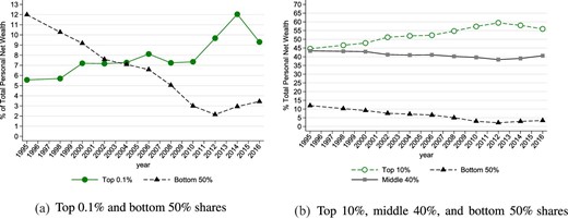
The inversion of fortunes between 1995 and 2016. The graphs show the shares of total personal net wealth accrued by the bottom 50% of the adult population (25 million individuals in 2016) ranked by total net wealth, the richest 0.1% (50,000 individuals), the top 10%, the middle 40%, and the bottom 50%, benchmark definition.
Our series are also triangulated with external evidence: namely Forbes rich list (which tracks the evolution of the share of the five richest individuals since 1988, and the richest 10 since 2001) and Credit Suisse Report (Davies, Lluberas, and Shorrocks 2017), both of which are broadly consistent with the evidence assembled here.
The use of tax data entails costs and requires adjustments. These include aligning real estate valuations with market prices, converting decedents’ distribution to living wealth holders using the mortality multiplier method, estimating the wealth of the unidentified population through household surveys, and addressing non-taxable assets and potential under-reporting.
The benchmark approach in this study is to fully distribute the household sector’s balance sheet from NA. While acknowledging that the balance sheet might not provide precise figures (as discussed in Section 2), it serves as a reasonable indicator (enshrined in official statistics) for tracking aggregate development over time and allows for better cross-country comparisons. However, this requires imputing unobserved wealth from tax records and household surveys. In any case, we also present series based on tax and survey data before imputations, as well as series that incorporate unreported offshore wealth and household durables. In our view, this multi-series approach, that is, one that offers the opportunity to compare information from different and competing data sources, is preferable to the alternative option of looking at one and only one series resulting from the combination of those sources.
Our benchmark series thus emerges from a wider range of values, representing different methods of estimation. This approach demonstrates that the key findings regarding wealth concentration evolution in Italy are not solely driven by the imputations. It also enables comparisons with historical series that are not scaled to the NA (Gabbuti and Morelli 2023 for Italy; Piketty, Postel-Vinay, and Rosenthal 2006 for France; Alvaredo and Saez 2009 for Spain; Alvaredo, Atkinson, and Morelli 2018 for the UK; and Roine and Waldenström 2015 for Finland, Norway, the Netherlands, Sweden, and Switzerland etc.) as well as to recent work on the US, France, Spain, and Germany (Saez and Zucman 2016; Batty et al. 2019; Garbinti, Goupille-Lebret, and Piketty 2021; Martínez-Toledano 2017; Albers, Bartels, and Schularick 2020), which follows the Distributional National Accounts (DINA) framework (Alvaredo et al. 2016, 2020).
The level of wealth concentration observed in Italy appears to be in line with other European countries; however, its evolution over time is closer to that found in the US, showing a sharp increase in recent years. By contrast, whereas the share of Italy’s middle 40% (P50–90) remains relatively high, the share of the bottom 50% experienced the strongest decline since the mid-1990s when compared with other countries.
The paper devotes substantial space to discussing measurement. It also sheds light on the determinants of the wealth inequality trends revealed by our analysis, thus making important contributions to the literature.
First, our estimates suggest that age and life-cycle factors do not explain the current level of wealth concentration. Second, we document how the heterogeneity of portfolios across the distribution influences the dynamics of wealth concentration. Whereas housing wealth plays a significant role for the middle 40% group, the accumulation of wealth at the top is primarily driven by financial and business assets. Moreover, changes in currency and deposits, along with increasing levels of indebtedness, contribute significantly to the net wealth dynamics of the bottom 50% group. Third, we investigate the relative role of savings and asset prices. Our results show that changes in total savings (defined as the sum of direct changes in the volume of indebtedness, deposits, and valuables, and any residual changes in the asset value that is not accounted for by changes in the asset prices) account for a very large portion of growth in net wealth, both in the overall population and within the top decile. Interestingly, this occurred despite a sustained declining trend in the saving capacity of households over recent decades.
Our analysis of the joint distribution of income and wealth also reveals that the probability of top 1% and top 0.1% of labor income earners climbing to the top 1% of the wealth distribution doubled between 2001 and 2014. Although changes to asset prices are not the predominant force behind the increase in wealth concentration, certain interesting findings are worth noting. Our results show that little of the change in wealth recorded between 1995 and 2016 across the distribution can be attributed to changes in house prices.4 On the contrary, changes in equity prices account for a large share of wealth growth above the 99th percentile and are practically irrelevant in the middle and bottom parts of the distribution (with the exception of the 1995–2008 sub-period). Lastly, we present new evidence on the increasing significance of wealth transfers, such as inheritance and inter vivos gifts, as well as their growing concentration at the top. Moreover, we find that wealthy inheritors have experienced a decreasing tax burden over the past two decades, following tax policy changes that have undermined the progressive nature of inheritance and gift taxes. These changes in the patterns of wealth transfers and their impact on long-term wealth concentration dynamics have been overlooked in empirical studies.
The paper is structured as follows. The second section describes the concept of net wealth and the nature of the aggregate wealth of the household sector. Section 3 dwells on the structure of the inheritance tax in Italy, the currently available data, and the mortality multiplier method. It goes on to describe the valuation of specific asset classes as well as the wealth of the missing population and tax-exempt assets. The fourth section presents our main empirical findings on the evolution of wealth inequality and concentration in Italy, including the comparison of our estimates with those available in other countries. The fifth section triangulates our evidence with that of alternative sources of data. Section 6 discusses the role of different factors in driving wealth concentration in Italy. Our final section briefly presents a series of robustness checks. Our concluding remarks follow.
2. The Macro Dimension: The Growing Relevance of Personal Wealth in Italy
According to the national balance sheets, Italian households are among the wealthiest and least indebted of the rich economies. Net wealth per capita, taken as the sum of all financial and real assets minus liabilities, was €21,000 (2016 prices) in 1966. By 2006, just before the onset of the financial crisis, this figure had increased eight-fold to €164,000. As shown in Figure 2, it then dropped to €141,000 in 2016. A fall as remarkable as 14% did not occur in any of the other advanced economies with the exception of Spain.
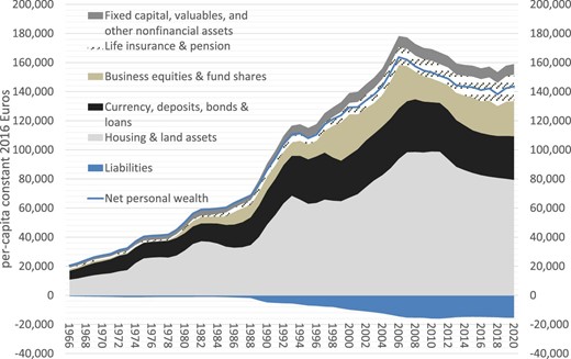
The growing relevance of households’ per capita net wealth. The graph shows stacked estimates of five different asset classes (Housing and land; currency, deposits, and bonds; directly held shares in listed and unlisted corporations, other equity in quasi-corporations, and investment fund shares; life insurance reserves and the balance of private pension funds; fixed capital and other non financial assets of small personal businesses of producer households (such as plant, machinery, equipment, inventories, and goodwill); and liabilities held by the household sector excluding the non-profit sector serving households). The series assembles data from the balance sheets and the financial accounts from the Bank of Italy, ISTAT, and WID.world. The blue line in the graph shows the evolution of households’ net wealth derived from the sum of all asset classes minus all liabilities. Online Appendix A provides more information about how we reconstruct the series.
Over the past five decades, housing and land assets accounted for about 50% of personal sector wealth. Official balance sheets, published jointly by the Bank of Italy and ISTAT, only cover the household sector including non-profit organizations. As detailed in the Online Appendix A.3, our analysis focuses on the household sector. The value of direct equity holdings, investment funds, and indirect financial securities through life insurance and private pension funds increased as a proportion of total gross assets, from 14% to 23%. Savings, current accounts, currency, and bonds declined from 24% to 17%, as did the value of fixed capital, valuables, and other non-financial assets from 5.8% to 3.5%. Personal debt, worth €15,000 per capita, almost doubled as a share of total gross wealth since 1995. Despite this, Italy maintains one of the lowest indebtedness levels currently recorded in the rich world, in contrast to the situation of the debt of the public sector.
Italy also has one of the highest ratios of private wealth to national income. Over 7 years of national income would be needed to account for the net worth of the household and non-profit sectors. This ratio was 2 around 1970. It is now close to 6 in other rich countries like France, Japan, and the UK, and to 5 in the US and Germany.
To understand this context in more detail, we now discuss the concept of net wealth and present current challenges to its accurate measurement, including the exclusion of particular assets, and the undervaluation of non-marketable assets and property wealth.
The Meaning of Net Wealth.
Wealth holding, by shaping one’s current and future consumption and earning potential, represents a unique determinant of the well-being and the living standards of individuals and households. The implications of wealth holding go well beyond the direct effects on consumption opportunities. Specific assets, such as company shares, may convey direct or indirect control over productive resources and, similarly, may also provide substantial power of influence in society as well as a clear mark of status. The level of individual wealth holding also affects risk-taking behavior, and can grant or deny access to specific investments, education, or job opportunities. Hence, the aggregate level of wealth, its composition, and its distribution together affect the functioning of the economy and the structure of society, and may also guide the structure of tax policies.
The central concept of net wealth employed in this paper refers to the current value of all tangible and intangible assets that are under the control of the households, which provide economic benefits to the holders, and over which property rights can be exercised. The assets may be financial, such as current or savings accounts, stocks, bonds, financial assets held in private pension accounts, and life insurance reserves, or they may be real assets, such as land, houses, non-residential buildings, and tangible and intangible fixed capital (plant, machinery, equipment, inventories, goodwill, software, and intellectual property rights). Thus, our definition of personal net wealth is aligned with that of the 2008 SNA (UN 2010) and the 2010 European System of Accounts (EU 2013). The latter definition is grounded in conventional, neoclassical economic theory, where wealth represents a store of value for present and future consumption. It is worth stressing, however, that there is no unique definition of wealth, and that the methods of valuation matter substantially.
The definition of wealth under the SNA excludes certain assets that are particularly relevant for specific groups of the distribution. For instance, NA only imprecisely capture the wealth that households own outside of the country of residence, most likely leading to assets of high-end groups going unrecorded. In this paper, we carry out robustness exercises, which incorporate estimates of unreported offshore bank deposits and portfolios of financial securities.
Antiques, artworks, and valuables are included in the SNA definition, but consumer durables (vehicles, electronic goods, and other household possessions) are not. These are instead considered within the consumption section of the NA. These assets are generally more evenly distributed than total wealth, and their inclusion may reduce the estimated level of wealth inequality.5 In this paper, we include durables and household goods in alternative estimates of wealth concentration.
Furthermore, NA do not account for state pension wealth or unfunded defined benefit pension plans, which, instead, would likely add to the middle and the bottom of the distribution.6 However, the estimation of public pension assets is surrounded with considerable uncertainty: One needs to estimate the expected retirement age, the individual’s income pattern over the life-cycle, and the evolution of pension tax policies; the net present value is also influenced by the choice of discount factor as well as the life expectancy of each individual and the mortality probability of their spouse. Moreover, future benefits from public pensions cannot be disposed of, transferred in full to other people, or used as collateral, and are not under the control of the rights holders. Hence, the exclusion of public pension assets can be justified if the research objective is to study the distribution of wealth from the perspective of the control over productive resources or the concentration of power. However, when the objective of the research is to study the inequality of welfare over the life cycle, the exclusion of public pension assets is harder to justify; pension assets provide financial security and can significantly influence behavior as people can substitute future claims with alternative forms of savings accumulation in order to face future consumption needs (Feldstein 1974). Saez and Zucman (2016) argue that “although social security matters for saving decisions, the same is true for all promises of future government transfers. Including social security wealth would thus call for including the present value of future Medicare benefits, future government education spending for one’s children, etc., net of future taxes” (p. 526). In this paper, we do not attempt to include future public pension or any other future claims from government services. Only assets held in private (defined contributions) pension plans are considered. But the debate is not settled.
The second key limitation of the SNA stems from its market valuation of asset: The cash value that can be recovered (and therefore consumed) by selling a given asset on a well-functioning market. Such a method is problematic for assets that cannot be put on sale, either because a market does not exist or because the asset itself may not be marketable. This is a valid qualification for life insurance plans, which cannot be easily accessed for liquidation. However, private reserves that insurers are required to hold for the future payment of life insurance benefits are included in the balance sheet within the class of “insurance technical reserves.” This class of assets, fully accounted for in our benchmark series, also includes the private balance of defined contribution pension plans. Moreover, the reserves held by firms for future severance payments on behalf of workers are also included.7 A similar issue arises for shares in unlisted corporations or in unincorporated private businesses taking the form of quasi-corporations, as they may never be or have never been sold.8 Financial accounts report estimated market values of unlisted shares derived from looking at similar listed corporations in the same business sector. Similarly, estimates of the market value of shares in quasi-corporations are taken from their self-reported market valuation in the SHIW (this excludes the buildings).9
Our benchmark wealth distribution series are consistent with the personal sector balance sheets. Hence, the valuation of business assets adopted in the NA also applies to our final benchmark series.
The third important limitation refers to the valuation of housing stock. In Italy, housing wealth is “estimated as the product of three factors: (a) the number of dwellings owned by households; (b) the average floor area in square meters of dwellings; (c) the average price per square meter of the dwellings owned by households. The value of housing wealth is then increased by the value of public residential properties sold to households” (Banca d’Italia 2014, p. 19). In this paper, we derive a market value measure of housing stock based on individual cadastral values reported on tax records. Our independent aggregate value of the housing stock very closely tracks the total of the household sector balance sheet and, ultimately, our distributional estimates are fully aligned with the latter.
3. From the Wealth of the Decedents to the Wealth of the Living
3.1. Inheritance Tax in Italy
The inheritance tax (Imposta sulle successioni e donazioni) applies to all worldwide taxable assets inherited, net of liabilities and deductible expenses, from a deceased person domiciled in Italy.10 It applies to the amount received by each heir and not to the amount of total wealth left at death, as is the case for the estate taxes levied in the US or the UK. The tax rates vary depending on the degree of kinship. For spouses and direct descendants or ascendants, the rate is 4% above any net share above €1 million.11 Siblings are subject to a rate of 6% above €100,000. Relatives within the fourth degree, direct relatives in law, and side relatives in law within the third degree, are subject to a 6% rate with no exemption threshold; 8% applies to all other parties with no exemption threshold. The same rates and structure apply to inter vivos gifts.12 Until 2016, the exemption threshold was reduced by the value of the capitalized lifetime donations received by each heir from the same deceased person. This provision, known as the coacervo, aimed to limit tax avoidance through gifting by integrating the taxation of gifts and inheritance.13
Inheritance tax returns are mandatory for real estate transfers or if the estate’s net value exceeds €25,000. The tax administration is connected to the cadastral register, as other taxes apply to real estate transactions. With high homeownership rates, this ensures a coverage rate of over 50% of decedents. This remained true even during the period when the inheritance tax was abolished (2001–2006). In 2013, 365,000 estates out of 600,000 adult deaths were recorded, while 2014 data shows a record-high coverage rate of 63%. Although incomplete, a coverage rate over 60% is very high compared with the evidence from other rich countries: In the UK, this number is below 50%, whereas in the US it is lower than 0.5%.14 A variety of exemptions permit the reduction of the effective tax bill beyond the statutory description. Many assets are exempt from taxation: reserves accumulated in private pensions, life insurance funds, shares of family businesses passed to a surviving spouse or direct descendants, postal savings bonds, and government bonds. The tax-exempt status implies, in many cases, that such holdings are not reported in tax returns and need to be partially or fully imputed. The treatment of tax-exempt assets is discussed in the next section.
Three major reforms were enacted in 2000, 2001, and 2006. Before 2000, the tax was a mix between a progressive estate tax (with marginal rates ranging from 3% to 27%), and an inheritance tax (with a further graduation of marginal rates up to 33%) that applied only to recipients other than the spouse and direct relatives.15 In 2001, the inheritance and gift taxes were abolished, before being reintroduced in 2006.
3.2. The Inheritance Tax Data
Our data are sourced from the universe of inheritance tax returns filed between 1995 and 2016 (evaluated at the year of death). Executors of the estates submit the returns within 12 months of the death.16 These returns are processed by a designated official at the local tax authority branch, who assesses the tax liability. The process also involves verifying legal ownership and obtaining third-party asset valuations, which improves the accuracy of the information and minimizes opportunities for tax evasion.17
The net wealth of the decedent is obtained by adding all reported financial and real assets and subtracting all liabilities. We add to this the market value of assets sold within 6 months from death, which was reported between 1990 and 2000; this is typically negligible.
The statistical office of the Ministry of Economics and Finance transformed the microdata into detailed tabular form. The tabulations have 34 net wealth ranges, from negative values to the highest range worth €20 million or more. Accompanying demographic information is provided by seven 10-year age groups (i.e., from under 20 to over 80), two gender groups (males and females), and three geographical areas (south and islands, north, and center).18 Four asset classes are identified: housing and land; business assets, equity, and debt securities; other assets (including current and saving deposits, valuables, etc.); and liabilities and deductible expenses.19 The data, therefore, lump together all business assets (including assets from personal businesses) with financial assets. The tabulations identify the taxes paid (on the global value of the estate as well as on the inherited shares), the value of assets sold within 6 months of death (reported between 1990 and 2000), and the capitalized value of all gifts and donations made during the deceased’s lifetime.
3.3. The Application of the Mortality Multiplier Method, the Estimation of Missing Wealth, and the Treatment of Different Assets
The distribution of the taxable wealth of decedents, generated from inheritance tax data, is different from that of the wealth of the living. A number of adjustments are therefore required: differential mortality multipliers must be applied in order to transform the estate data into estimates of wealth-holding; likewise, an estimate of the wealth of those not covered by the tax (the missing wealth of the missing/non identified population), as well as that of the exempted assets, is needed; and, finally, real estate valuation must be converted from cadastral to market prices. In this section, we also discuss the estimation of personal wealth held in trusts and the valuation of business assets as well as the treatment of liabilities. A summary of the treatment of different assets in the tax records and in our benchmark series can be found in Online Appendix R.
Re-weighting the Population of the Deceased.
In 1995, 30% of Italy’s estates belonged to individuals aged 80 and above; in recent years, the number has grown to 60%. Similarly, males are over-represented across all age groups, except the oldest group. To re-weigh the decedent population, we apply mortality multipliers, obtained by inverting the mortality rates, which are therefore treated as if they were sampling rates of the living population. The application of mortality multipliers has a long tradition in economics and statistics and leads to the derivation of the identified wealth and population (for a description of the method; see Atkinson and Harrison 1978). We also use detailed annual mortality tables published by the ISTAT, available for each age, gender, and geographical location.20
The inverse of the mortality rate of each decedent group i (for which the multiplier is defined as mi ≡ 1/pi, and where pi is the mortality rate of group i) represents the number of living individuals with similar socio-demographic characteristics. We multiply the number of decedents and their reported wealth value by the relevant mortality multiplier mi for each group i.
We define the estate value of each decedent as wE,i, arranged in descending order, so that wE,i ≥ wE,j, if i < j. The population of decedents is NE and the total value of their estates is defined as WE, taking the following form: |$W_E = \sum _{i=1}^{N_E} w_{E,i}$|. The application of the mortality multiplier provides the following result: |$W = \sum _{i=1}^{N_E} m_i w_{E,i}$|, where W is the total wealth among the living population.
Given the large number of decedents covered, the re-weighting of tax records allows us to account for a substantial fraction of the living population (50%) and personal net worth (80% of NA in recent years, and 65%–70% in the mid-1990s), where this includes only the correction of the market price of housing assets. The total net wealth in the SHIW, representative of the entire population, is instead very similar to that identified from tax records between 1995 and 2006; however, from 2006, it only accounts for 65%–70% of the NA total.
The Wealth of the Missing Population.
The tax data are representative of the living adults whose wealth arrangements are such that they only come to the notice of the tax authority in the event of their death. The need to estimate the amount of missing wealth is a necessary step if we want to assess the size and distribution for the entire population. The SHIW is the basis for this. In order to be consistent with the distribution at the individual level, we first allocate household wealth to adult members of the household.21 We then estimate that 50% of adults are accounted as missing, with strong heterogeneity across age groups.22
Once the missing population and their wealth holdings are estimated, we can impute these values to the tax-based distributional information. Online Appendix H describes the very simple imputation process and shows that the estimated missing wealth amounts to €700 billion and it is mostly composed of deposits and valuables.
The Valuation of Real Estate.
To address the undervaluation of land, buildings, and dwellings for tax purposes, we adjusted cadastral values to align with market prices.23 The adjustment factor is calculated as the ratio of average market price (Osservatorio del Mercato Immobiliare—OMI, published by the Revenue Agency/Nomisma) to cadastral valuation at the national level. From 2009 to 2012, this ratio remained stable at 3.3, but declined to 3.2 in 2013, 3.0 in 2014–2015, and 2.9 in 2016. See Online Appendix E for the time series of adjustment factors.
Most notably, the simple re-scaling of property values using an annual market to cadastral value ratio generates a total housing and land stock very close to that estimated in household sector balance sheets (the average estate valued at market prices increased from €209,000 in 1995 to €332,000 in 2007 at 2016 prices; it remained relatively constant until 2012, and then started to decrease to €293,000 in 2016). Due to the structure of inheritance tax filing, as well as the prevalence of homeownership in Italy, the number of inheritance tax filers who declare real estate assets is above 90%. Similarly, the declared estate is mostly composed of real estate assets: whereas in 1995, 91% of estates were composed of housing and land, by 2016 this fraction had declined to 78%. This was also the result of the tax exemption of a number of financial assets. However, the high share of housing and land does not mean that our data are unable to capture large financial wealth holdings at the very top of the wealth distribution. Indeed, as reported in Acciari and Morelli (2022), “in 2016, only 10% of total gross estate is composed of housing and land for the group of richest 0.01% of total decedents, a group whose total declared net estate is at least €17 million. For this group, nearly 90% of total gross estate value is held in financial securities and privately held business assets. Meanwhile, for estates below the 99th percentile, housing and land account for at least 75% of total gross estate value.”
The use of a national multiplier runs the risk of masking the heterogeneity across geographical areas and, most importantly, across the wealth distribution (e.g. the degree of underestimation of real estate market values could be more pronounced for rich individuals). To address this concern, we run a number of checks matching the full cadastral records of over 34 million properties to the corresponding OMI market value of the area, as well as to the income tax statistics for over 32 million tax payers (the OMI market value is the average market price of the micro-zone where the real estate is situated). Checks are also carried out by integrating the EU-SILC survey with administrative data from the cadastre and OMI market value data (carried out internally at the Ministry of Economy and Finance through a microsimulation model). These exercises are detailed in Online Appendix E.2. Our main findings suggest that although the full heterogeneity across locations and rankings in the income distribution is ignored, the use of a national multiplier should only marginally affect estimates of wealth concentration. Our results are likely to represent conservative estimates, as controlling for the heterogeneity discussed above would have likely increased the level of wealth concentration even further, albeit marginally.
Tax-Exempt Assets.
Italian legislation grants full exemption to financial assets invested as private pension and life insurance, postal saving bonds (i.e., Buoni Fruttiferi Postali), and a number of national and extra-national government securities.24 The list of exempted assets also includes vehicles on the national registry, credits toward the state, properties that are listed as cultural and historical heritage, and family businesses and control shares of private businesses that are transferred to direct descendants or to a spouse.25 The value of tax-exempt assets considered here, imputed to the population, is taken from the household sector balance sheet as the value of insurance technical reserves net of their liabilities (i.e., the value of assets accumulated in pension, life insurance, and severance payment funds), plus 50% of Italian government securities; they amounted to €320 billion in 1995 and €940 billion in 2016, equivalent to 11% of household net wealth (see Online Appendix H.2). The reporting of government bonds is often advised by tax accountants and frequently occurs in those cases where securities are bundled together with other assets within investment funds (e.g. banks and other financial intermediaries are required to provide detailed descriptions of investment funds and accounts following the death of a legal owner). Such investment bundles can be fully reported on the inheritance tax form, so that the tax authority could then compute the relevant tax deductions.26
Business Shares and Equities.
The total value of business assets held by households is composed of the sum of the shares in corporations and quasi-corporations. Our tabulations bundle business assets with other financial assets such as mutual fund shares and bonds. The final valuation of business assets adopted in our benchmark distribution series is consistent with personal sector balance sheets. Hence, shares in corporations and quasi-corporations are included at market value. To do so, the value of any “shares and other equities” as an asset of the household sector balance sheets that is not accounted for in our inheritance tax-based data is distributed to the whole adult population as a proportion of the total “financial assets” across each age, gender, and location cell. Note that this method also applies as we distribute the value of plant, machinery, equipment, inventories, and goodwill of small personal businesses of producer households. Differently from shares in corporations and quasi-corporations, these are real assets listed as “fixed capital” in the balance sheet, and are valued at substitution price net of depreciation. See Online Appendix A.4 for an account of business assets in the macroeconomic accounts.
Trusts.
Trusts are not taxable under the inheritance tax, as the property of the settled assets is transferred from settlors to trustees. Very little is known about the amount of wealth held in trusts in Italy, but their use is not as widespread as in the US or the UK. According to data from the Ministry of Economy and Finance, the number of trusts operating in Italy required to file a tax record increased from 65 in 2009 to 151 in 2019 (14 of which were foreign trusts). Using the universe of income tax files allows us to observe the capital incomes from trusts (national and foreign) that are imputed to individual resident beneficiaries (transparent trusts), as well as those that are retained in opaque trusts (Redditi da capitale imputati ai trusts). On average, 89% of the capital incomes of trusts are reported to be distributed to beneficiaries. We capitalize those capital income flows to arrive at a value of €166–332 million for 2015 and €263–526 million for 2019.27 In 2016, these wealth value estimates only accounted for 0.002%–0.005% of wealth (see Online Appendix Q). These values almost certainly represent a lower bound, as capital incomes are often subject to separate withholding taxes and may be under-reported in Italian income tax records. Yet even doubling the estimates of total wealth held in trusts would not change the fact that such assets would only have a negligible effect on the distribution of personal wealth, even if they were imputed entirely to the wealthiest groups.
Liabilities.
The concept of net worth used in this paper subtracts all liabilities from real and financial assets. The existence of very high tax exempt thresholds reduces the incentive for detailed reporting of liabilities for most (non-taxable) estates. To overcome this limitation, in our benchmark series, the unobserved value of liabilities reported in the national balance sheets is imputed proportionally to the population according to the distribution of liabilities reconstructed from the tax data, complemented with observations about the missing population, using the survey data as described above.
A less relevant limitation of tax records comes from the fact that liabilities may be reported together with deductible expenses, which include the costs of a funeral or medical treatments during the last 6 months of the deceased person’s life. While it is not possible to appropriately add the deductible expenses back to the value of the individual estate, the entity of these expenses is negligible (e.g. only a small fixed amount of funeral costs that can be deducted for tax reasons but no specific threshold is specified for health related costs).
3.4. Combining Different Sources of Data
The process of adding the wealth of the identified population (including the price adjustment to real estate), the wealth of the missing population, and the imputation of exempted assets, shown in Figure 3, generates a total wealth that is between 80% and 100% of the balance sheet of the household sector in the NA, with very similar trends.
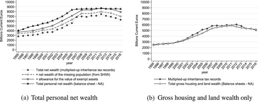
Total personal net wealth and total gross housing and land wealth: from inheritance tax records to NA. Panel (a) compares the different wealth aggregates, from that identified using the estate multiplier method (scaling-up the reported wealth at death), with the total net wealth of the household sector from the national balance sheets. Panel (b) compares the total gross value of the housing and land stock as identified from the inheritance tax records with that reconstructed from the balance sheet of the household sector from the NA.
In seeking to align the benchmark series to the NA, the remaining gap of total assets and liabilities must be imputed. This benchmark approach is justified on the grounds that the NA provide a reasonable indicator of the development of wealth over time, preserving a high degree of cross-country comparability, rather than on the assumption that the NA give the correct numbers. On the one hand, the imputation of the wealth gap is a controversial exercise, riddled with difficulties and uncertainty. On the other hand, the adjustment to NA is advantageous in that it deals indirectly with any residual misreporting, mis-valuation, or tax avoidance and evasion ignored in the preceding steps. In any case, it should be stressed that some of the difference between NA and other wealth data sources are rooted in definitional issues rather than quantitative misalignment.
For all these reasons, we will also discuss the variety of ways in which estimates behave once we deviate from the benchmark (e.g., excluding imputations). This type of exercise has not commonly been reported in previous studies of wealth inequality; however, we argue that it is essential to increase transparency about how final measures of concentrations are derived, and should not be relegated to a marginal appendix.
4. The Growing Inequality of Wealth Holdings
4.1. Benchmark Series
Similarly to using household surveys, one of the immediate advantages of our benchmark approach over the strict application of the estate or the capitalization methods is the potential to analyze the size distribution for the whole population. We can show how the shape of the wealth distribution has changed over time. As illustrated in panel (a) of Figure 4, the Lorenz curve shifted outward from 1995 to 2016. Panel (b) plots the difference between these two curves over time. The difference is always negative for every wealth group, as the Lorenz curve in 2016 always lies below that of 1995. Therefore, any possible standard indicator would point in the same direction: Wealth inequality has increased in Italy over the time period considered.28
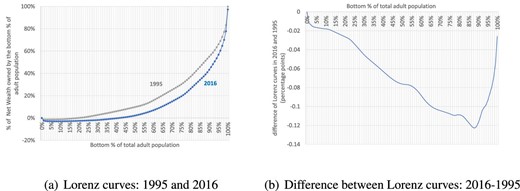
Increasing wealth inequality over time. Panel (a) compares the Lorenz curves in 1995 and 2016. Panel (b) shows the difference between these two Lorenz curves.
We illustrate this point with the evolution of the Gini coefficient, which recorded a 14 percentage point increase, from 62% in 1995 to 76% in 2016 (see Online Appendix A.2). This is a substantial change if compared with results from SHIW data (Figure 7).
We now zoom in on the upper wealth brackets. The top 1% (adults with at least €1.5 million and average net wealth holdings of €3.8 million) controlled about 22% of net wealth in 2016, a share that has increased by 6 percentage points since 1995 (Figure 5). Panels (a) and (b) of Figure 5 also demonstrate the importance of looking within the top 1%, as top groups are highly heterogeneous. The share of the top 0.01% more than doubled between 1995 and 2016, increasing from 1.8% to 5%. Such a tiny group held 500 times their proportionate share in 2016, with a minimum net worth of €20 million and average net worth of €83 million, equivalent to 470 times the average net worth. The share of the top 1% excluding the top 0.01% rose gradually from 1995 to 2012, increasing from 14.4% to 19.0%, before declining again and stabilizing around 17%.
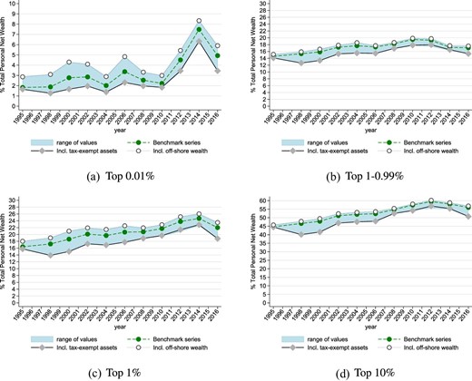
The evolution of top wealth shares. Italy 1995–2016. The graphs show the evolution of the shares of total personal net wealth for four subgroups of the adult population between 1995 and 2016. Each panel shows three series. The middle line is the benchmark (distribution of balance sheets). The upper line, after adjustment to NA, also includes unreported offshore financial assets. The lower line, instead, only allows for tax exempt assets.
The ranges of values depicted in the figures (which are not confidence intervals in the statistical sense) signal that the adjustments required to reach the benchmark series are not the only ones that can be adopted. Yet the estimated wealth concentration and its evolution remain robust regardless of the inclusion or exclusion of our adjustments to the data. The bottom of the range is derived by imputing only tax exempt assets: falling short of fully imputing all missing assets and liabilities required to align distributional estimates to the household balance sheet as shown in our benchmark case. The upper limit, instead, imputes even more assets than our benchmark case by also including unreported financial assets held in offshore tax havens.
Unreported Offshore Wealth.
A fraction of financial wealth remains unreported or unrecorded in official statistics and tax agencies. Zucman (2013) argues that this represents 10% of world GDP. Applying similar methods, Pellegrini, Sanelli, and Tosti (2016) estimated undeclared debt and equity securities in Italy to be €161.4 billion in 2007, excluding undeclared bank deposits. Figures on undeclared bank deposits held by the non-banking sector in offshore centers are also reported in Pellegrini, Sanelli, and Tosti (2016), based on the cross-border banking statistics released by the Bank of International Settlements. We assume that half of the latter belongs to individuals, and from this allocate to Italy the country’s share of global GDP.29 The resulting estimate of unreported financial wealth held offshore by Italian investors is €187.2 billion in 2007, or some 2%–3% of personal wealth.30 We further extrapolate backward and forward according to the evolution of the European offshore financial wealth given in Alstadsæter, Johannesen, and Zucman (2018), to cover the period 1995–2016.
If we assume that the share of undeclared wealth and its relative distribution across the wealth distribution in Italy is the same as what was estimated for Denmark and Norway by Alstadsæter, Johannesen, and Zucman (2019), then the share held by the top 1% increases by 1–2 percentage points throughout. This is a significant effect that becomes even more visible at the very top. The richest 0.001% of individuals saw their share increase by 65% in 1995 (from 1.8% to 3%) and by 14% in 2016 (from 5% to 6%). The inclusion of unreported offshore financial wealth is surrounded by much uncertainty; however, it does not appear to substantially affect the trend of the concentration over the period studied.
4.2. Comparison with other Countries
Our benchmark series are currently comparable with the wealth concentration estimates available for France, Germany, Spain, and the US (the comparison with existing country series that do not follow the strategy of up-scaling to the NA is given in Figure 16(b)). Figure 6 displays three concentration indicators: the top 10%, the bottom 50%, and the middle 40%. Italy, in the mid-1990s, had one of the (relatively) best-positioned middle 40% groups, and one of the lowest concentration levels. Similarly, the bottom 50% held 12% of wealth in 1995 compared with 8% in France, 7% in Spain, 5% in Germany, and 1% in the US. Twenty years later, Italy appears to have experienced the largest drop in total wealth held by the bottom 50%, and, although the levels of wealth concentration are now closer to those of other European countries, its relative increase over time bears more similarity to the dynamics of the US. However, the middle 40% in Italy controls 40% of total net wealth compared to 30% in the US.
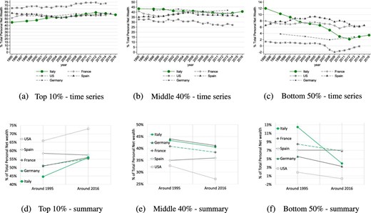
Wealth concentration: a cross-country comparison. The figure compares the evolution of wealth inequality from c.1995 to c.2016 for countries for which we have series comparable to our benchmark. Italy is based on the authors’ results, Spain comes from Martínez-Toledano 2017, France from Garbinti, Goupille-Lebret, and Piketty 2021, Germany from Albers, Bartels, and Schularick 2020, and the US from Saez and Zucman 2016. “Around 1995” refers to 1995 for all countries except Germany (for which it refers to 1993). “Around 2016” refers to 2014 for France and the US, to 2015 for Spain, to 2016 for Italy, and to 2018 for Germany.
The notable decline in the share of the bottom 50% may seem surprising from the perspective of the given international comparison. However, it is consistent with the sizeable increase in Italy’s aggregate wealth and with the fact that this group has not benefited proportionally from the factors pushing average wealth upwards: They own zero-return financial assets, have very little net real estate, or are heavily indebted mortgage-wise.
5. Triangulation with other Sources
We now consider external evidence based on a variety of sources, from household surveys to rich lists and banking sector reports.
Household Survey: Evidence from SHIW Data.
Data from SHIW provide essential information about the distribution of Italian households’ wealth since 1989. A comparison with tax data requires changing the unit of analysis from households to individuals. Household wealth must be allocated to each adult member using the relevant information from the survey questionnaire, as done in D’Alessio (2018) and mentioned in Section 3.3. Furthermore, to bring the estimate in line with our concept of wealth, an estimate of private insurance funds and pension assets are added to individuals declaring payments of any insurance premium or private pension contribution. As shown in Figure 7, moving from the household to the individual reduces the share of the bottom 50% by 5 percentage points (panel (b)), a large change, and increases the share of the top 1% by 2 percentage points (panel (a)). The concentration at the top is only marginally different if we split household wealth equally among the head of the household and his or her partner (equal-split series).
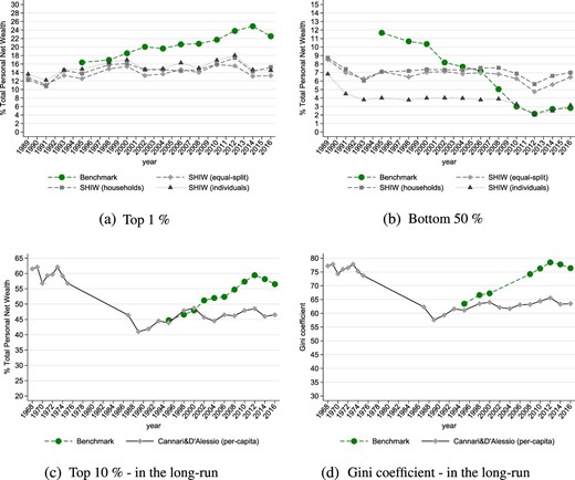
Gini coefficient, Top 1%, and Bottom 50% shares in total wealth: comparing results with household survey data. Panels (a) and (b) show the evolution of the top 1% and bottom 50% shares from household surveys (SHIW) compared with our benchmark series. The comparison requires adjusting the wealth concept and the unit of analysis (from households to individuals). Panel (c) compares the evolution of our benchmark series of the top 10% with that from Cannari and D’Alessio (2018b) based on the combination of the SHIW and historical surveys from 1968 to 1975.
The levels and dynamics of wealth concentration are very similar across tax- and survey-based estimates until 2000, when they begin to diverge. According to the SHIW, the top 1% share remained roughly constant between 1995 and 2016, however, according to our benchmark, it increased by 6 percentage points (Figure 7(a)). On the contrary, as shown in Figure 7(b), the share held by the bottom 50% is substantially higher in our benchmark series until 2004. The share of the bottom 50% becomes almost identical in both sources only from the mid-2000s onwards.
Different explanations can rationalize these complex findings. The under-representation of the wealth concentration at the top is not surprising. For a variety of reasons, household surveys are not necessarily well-suited to capturing the right tail of a highly skewed wealth distribution. First, in the presence of “fat tails,” such as the distribution of wealth, a random sample may not be fully representative of all wealth groups, especially if the sampling frame of the survey does not allow for the oversampling of wealthy households, as is the case for the SHIW. Second, even if very wealthy households were appropriately sampled, they might have a higher rate of nonresponse, as they may be harder to find or trace, or they might be less willing to cooperate to reveal their complex asset portfolios. The compliance rate may well be lower at the top of the wealth distribution, distorting the estimation of inequality indicators (Korinek, Mistiaen, and Ravallion 2007; Kennickell 2019; Muñoz and Morelli 2020). Indeed, the SHIW identifies fewer people and less wealth for the wealthiest ranges of the distribution compared with our multiplied-up estates from inheritance tax records (more details in Online Appendix F).31
Nonetheless, total personal wealth in the survey data amounts to 60%–70% of the balance sheets despite its implicit coverage of the total population (see Figure G.2 panels (a) and (c) in the Online Appendix). This indicates that underreporting of different types of assets and liabilities, as well as coverage issues, may also apply to the middle and bottom ranges of the distribution. The fact that the bottom 50% of the distribution appears so different in the survey data compared with our benchmark results may also indicate the inability of the survey to appropriately account for the most important form of assets for the lower groups, namely currency, deposits, and valuables. In our derived benchmark series, these assets constitute over 50% of the wealth of individuals with less than €15,000, that is, a substantial part of the bottom 50%. This stresses the need for better data to assess low-end segments of the wealth distribution, not just the high-end, as generally noted. The total value of currency, deposits, and bonds reported in the survey data was lower than that of NA-based data by a factor of 3.5. By 2004, the share of currency, deposits, and bonds stabilized at 20% of total net wealth in the balance sheet, by which point the survey underestimated the total NA value by 2.7 times. By 1995, however, the value of currency, deposits, and bonds accounted for 32% of total gross personal wealth in the balance sheet and the relative importance of this asset class declined, accounting for only 18% of total gross personal wealth in 2016.
More generally, the aggregate coverage rate of assets in the survey data, with respect to the NA statistics, is highly heterogeneous across asset types, ranging from 30% for liabilities and 35% for financial assets, to 85% for housing assets. The trend of these asset coverage rates has also changed over time: whereas little change occurred for housing assets, the coverage rate for financial assets and liabilities has been steadily declining over time. Figure G.2 (panels (b) and (d)) as well as Table H.1 in the Online Appendix document these patterns providing a more detailed decomposition of asset types.
Rich Lists and Banking Sector Reports.
Forbes magazine gives information on Italian billionaires; only 5 individuals were recorded in 1988, and 35 in 2019. The data are often based on journalistic estimates that can be subject to several types of errors, and the methodology used cannot be evaluated. According to Vermeulen (2017), parametrically adjusting the SHIW with the extreme observations from the rich list increases the top 1% share by 6–7 percentage points from a level of 14% in 2010. Applying similar methods and data from the Forbes World’s Billionaires, Davies, Lluberas, and Shorrocks (2017) imputed the “missing” upper-end of the wealth tail to household survey data for several countries from 2000. The same exercise is also carried out, on an annual basis, for the Global Wealth Report by Credit Suisse; their estimates from the mid-2000s appear to be in line with our benchmark series. Figure 8(a) shows this for the top 1%. These hybrid estimates seem to suggest that the correction of survey data for missing wealth, especially in the upper end wealth bracket, may prove a fruitful avenue for future research.
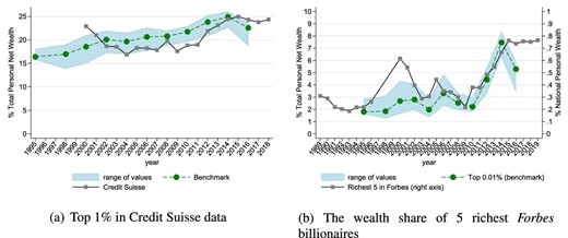
Triangulation of the evidence with external data series. Panel (a) compares the top 1% share of wealth from our benchmark series, from the Credit Suisse Report (combining SHIW data and Forbes rich list). Panel (b) compares the top 0.01% share of wealth from our benchmark series with that of the five richest individuals listed in the USD global billionaires rich list by Forbes.
We can track the share of total net wealth held by the Forbes richest five or ten individuals, from 1988 and 2000, respectively. As shown in Figure 8(b), a group whose size is a thousand times bigger (the top 0.01% represents 5,000 individuals) holds a share ten times higher. The dynamics of the Forbes list broadly concurs with our benchmark series. The five wealthiest Italians almost tripled their share of total wealth from the mid-1990s to 2016, from 0.2% to 0.7% (and the share remained at a similar level until 2019). The share of the top 0.01% also rose, from 2% to 7%.
6. Determinants of Wealth Concentration
Precisely identifying the channels that affect the evolution of wealth inequality has important implications for policy; however, the question remains broadly unanswered. Recent work in the US has emphasized that wealth inequality can be fueled by differential saving rates coupled with increasing income inequality (Saez and Zucman 2016). As discussed in Fagereng et al. (2019), richer households mostly “save by holding [...], meaning that they tend to hold on to assets experiencing persistent capital gains.” Indeed, a growing body of evidence stresses the importance of the heterogeneity of portfolio composition, asset prices, and rates of return across the wealth distribution (Alvaredo, Atkinson, and Morelli 2018; Fagereng et al. 2020; Benhabib, Bisin, and Luo 2017; Kuhn, Schularick, and Steins 2020; Advani, Bangham, and Leslie 2020; Martínez-Toledano 2020). Beyond these factors, individuals also differ in the extent of wealth transfers received via gifts and inheritances, as stressed in Feiveson and Sabelhaus (2018). It has also been suggested that the receipt of large inheritances may have a dis-equalizing effect, especially in the long-run (Nekoei and Seim 2018; Nolan et al. 2020). Reality is complex and certainly involves all the aforementioned elements, as well as others. For instance, Hubmer, Krusell, and Smith (2020) highlight how the decline of the progressivity of income taxes could explain the most important part of the dynamics of US wealth concentration since the 1980s. Other macroeconomic factors may well be very important too. Indeed, the period under analysis here is one of substantial economic turbulence, in which structural reforms to the Italian economy significantly affected the labor and credit markets, the public pension system, and a widespread program of privatization of state-owned corporations. As argued in Brandolini et al. (2018) “the currency crisis of 1992 is a watershed in Italy’s economic development. It marks the start of a phase of weak economic performance and uncertain growth prospects.” There are also concerns about the impact of the large Central Banks’ programmes of long-term bonds purchases, pursued in the US, the UK, and the EU following the Great Recession (Franconi and Rella 2023). To address these issues, this section explores some of the potential determinants of the trend of wealth concentration in Italy.
6.1. The Portfolio Composition across the Wealth Distribution and Wealth Dynamics
Workers save out of earned incomes during their working lives in order to dis-save through retirement and to face any other expected or unexpected needs throughout their life cycle. Moreover, for any given age group, different people across the income and wealth distributions may have different saving rates. Beyond this (obvious) accumulation channel, the existing stock of real and financial assets tends to reproduce itself; financial and real estate wealth may be invested, generating income returns that can be saved in turn. Positive real interest rates may accrue on bank accounts, and assets may also appreciate or depreciate over time, implying changes in the valuation of the stock of wealth independent of individual decisions to save.
The relative strength of each channel can vary over time and apply differently to different segments of the distribution. For example, Italy has experienced a marked decline in households’ savings rates out of disposable income since the mid-1990s, dropping from 16% in 1995 to 3% in 2016. During the same period, the interest rates on deposits decreased from 5.6% to 0.4%. Given that deposits make up a significant portion of total wealth for the bottom 50% group (along with valuables, amounting to at least 50% of gross wealth, Figure 9 in Online Appendix N.4), it is reasonable to expect a strong co-movement between the decline in saving rates and returns on savings and the wealth share of this group.
Additionally, the middle 40% and the top 10%–5% are likely to be particularly influenced by the dynamics of the real estate market because housing and land constitute the largest asset class for them (60% of total gross wealth in recent years as documented in Online Appendices Figure N.3(b) and N.3(c)). Between 1995 and 2008, the OECD house price index in Italy increased by 35%, closely following the growth in the average net wealth held by the middle 40%. However, after the 2008–2009 financial crisis, house prices stagnated and then declined, with the average house price decreasing by 27% by 2016. Between 2008 and 2016, the real average net wealth of the middle 40% declined by 12%.
Conversely, financial securities and corporate and non-corporate personal business assets have become dominant in the portfolios of the wealthy, particularly in recent years. In 2016, individuals with more than €20 million (the top 0.01%) held more than 80% of their wealth in the form of financial and business assets (see Figure 9). Hence, the reversal of house prices since the 2008 crisis, coupled with a fast rebound of stock prices, may have contributed to the substantial rise in wealth concentration at the top that we observe since 2010. Indeed, the OECD share price index for Italy declined by 59% between 2007 and 2012 and rebounded by 50% by 2015, before dropping again by 15% in 2016.
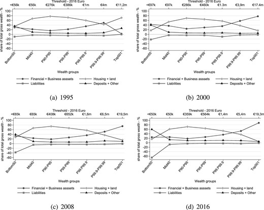
The composition of wealth across the wealth distribution. Adults are ranked by net wealth. Bottom, middle, and high-end groups are identified and total net wealth is decomposed into four classes: housing and land; business assets, equity, and debt securities; deposits and other assets (including cash, valuables, etc.); and liabilities. The top x-axis in each panel of the graph represents the monetary threshold (in 2016 Euro) to belong to each group. See Table N.1 in the Online Appendix for more details.
To further probe the role of heterogeneous portfolios and their returns, we use our data to show how different asset classes contributed to the rise in the concentration of wealth. For each group i, we define the share in total net wealth as Si, which in turn can be written as the weighted average of the housing (H) wealth share and the non-housing (NH) wealth share of the same group i. As discussed in detail in Online Appendix N.1, the exercise reveals (see also Figure N.1) that wealthy individuals have been capturing a growing share of non-housing wealth.
6.2. Decomposing Wealth Growth by Wealth Groups and Asset Types: The Role of Savings, Indebtedness, and Capital Gains
To better understand the proportional contribution of each asset class to the wealth growth of each wealth group P, we consider net wealth NW as the sum of each asset class Aj, housing and land (H), business and financial assets (F), and deposits and valuables (Dep), net of total indebtedness (D).
Following the work by Albers, Bartels, and Schularick (2020), we identify the contribution of each asset class to total wealth growth, over 1995–2016, by totally differentiating equation (1) and dividing by |${\it NW}^{P}_{t}$|.
Differently from Albers, Bartels, and Schularick (2020), we explicitly consider the composition of net wealth growth, and in doing so are able to isolate the contribution of indebtedness too. Online Appendix Table N.2 and Figure 10(a) and (b) highlight the heterogeneity of the results by wealth groups.
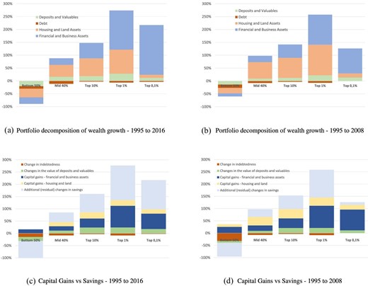
Net wealth growth decomposition across wealth distribution.
Between 1995 and 2016, housing wealth contributed 67% to the overall gross wealth growth. The relative contribution remains close to 60% for the middle 40%; however, it declines to 50% for the top decile, to 35% for the top 1%, and to 9% for the top 0.1%. On the contrary, the role of financial and business assets becomes much more prominent within the top percentile: It accounts for 57% and 85% of the growth of net wealth for the top 1% and the top 0.1 %, respectively (see Online Appendix N.2). Things are very different for the bottom 50% group, which lost 90% of its net wealth over 1995–2016, and for which declining values of currency and deposits and increasing levels of indebtedness account for a third of its net wealth change.
The Role of Savings and Capital Gains.
To further document the distinctive roles of the change in the volume of savings from that of the change in the price of assets, one needs only a simple law of motion of net wealth for each group P at time t, |${\it NW}^{P}_{t}$|:
where |${\it NW}^{P}_{t}=W^{P}_{t} - D^{P}_{t}$|, |$W^{P}_{t}$| is total gross wealth, |$D^{P}_{t}$| is the level of debt, |$\tilde{S^{P}_{t}}$| is total savings in period t net of all changes in indebtedness level for the group P, and |$q^{P}_{t}$| is the weighted average of price changes of asset j weighted by the average portfolio share of each asset j for wealth group P.
We then make use of the four components of net wealth available in our database, H, F, Dep, and D, assuming that all changes in the latter two classes are only the result of changes in volumes (savings), rather than in prices. Hence, only price changes for housing and land (|$q^{HP}_{t}$|) and for financial and business assets |$q^{FP}_{t}$| matter to our estimation if the role of capital gains. The accumulation equation can be rewritten as follows:
If one estimates the components associated with capital gains from housing and financial assets, changes in the indebtedness levels, |$\Delta {D^{P}_{t}}$|, and changes in direct savings under the form of deposits and valuables, |$\Delta {Dep^{P}_{t}}$|, one can define the residual change that reconciles the change in the wealth of group P. This residual category is defined as residual savings, |$RS^{P}_{t}$|, and we can interpret this variable as the variation in wealth resulting from changes in the volumes of housing and financial assets.
In line with existing literature (Saez and Zucman 2016; Kuhn, Schularick, and Steins 2020; Albers, Bartels, and Schularick 2020), the resulting savings flows would be considered “synthetic” as they are derived under the assumption of no mobility of individuals across wealth groups.
This exercise requires information about changes in prices. Following work by Albers, Bartels, and Schularick (2020), we use the observed portfolio composition of each wealth group P, and the OECD cumulative changes in the share price index and the house price index.32 We repeat this exercise over four different sub-periods: 1995–2000, 2000–2008, 2008–2012, and 2012–2016.33 This allows us to decompose the cumulative wealth growth across wealth groups during the whole period, between 1995 and 2016, and between 1995 and 2008, right before the onset of the financial recession.
Results are presented in Table N.3 and Figure 10(c) and (d) for the bottom 50%, the middle 40%, and the top 10%. To illustrate further heterogeneity, the top 1%, and the top 0.1% are also shown. Two main sets of findings are worth highlighting.
First, relatively little of the change in wealth recorded between 1995 and 2016 can be attributed to changes in house prices. This is due to the fact that house prices rose substantially until 2008 and then declined, meaning that the cumulative capital gains of the period were very small. The role of capital gains of housing assets becomes more prominent if we restrict the analysis to the upper middle class (middle 40%) and to the sub-period preceding the great financial recession. On the contrary, the total wealth of the top 1% increased by more than 250% from 1995 to 2008, with 36% of this growth attributable to changes in the price of financial and business assets. The percentage grows to 44% for the top 0.1% group.
The second main set of results follows. Our analysis suggests that changes in net wealth are predominantly driven by volumes and not by changes in the prices of financial and real assets. The bottom 50% group experienced a 90% decline in net wealth between 1995 and 2016. For this group, increasing indebtedness and, most importantly, declining deposits and volumes of housing and financial assets account for the bulk of overall change in wealth. At the very top, the net wealth of the top 0.1% grew by almost 300% over the same period, with over 75% of such growth being driven by changes in the volume of real and financial assets, as well as increases in deposits and valuable assets. Restricting the analysis to the period preceding the onset of the great financial recession highlights the more significant role of capital gains, especially at the top of the distribution.
It is worth noting that the use of external share and housing price indexes to derive “synthetic saving rates” for different wealth groups does not preserve the consistency with the NA framework. Also, diverging from Mian et al. (2020) and Bauluz, Novokmet, and Schularick (2022), we made no allowance for corporate retained earnings in our definition of savings. We discuss these methodological choices in Online Appendix N.2.
Interestingly, changes in the volumes of assets and savings continue to play an important role even with no allowance for corporate retained earnings, including at the top of the distribution. Moreover, the role of changes in the volume of assets remains strong despite a sustained trend of the saving capacity of Italian households declining over recent decades. Whereas the household saving rate as a percentage of disposable household income was one of the highest in the world in 1995 (16%); it declined to moderate levels at 3.2% in 2016. Using the SHIW, we estimated the gradient of household saving rates (defined as the difference between disposable income and consumption as a proportion of disposable income) with respect to the ranking of household along the net wealth distribution. We preserved this gradient but adjusted the estimated levels of saving rates to account for the proportional difference between the aggregate saving rates estimated in survey data and OECD macroeconomic statistics. The results averaged out for the 2000–2006 and 2008–2016 periods are presented in Figure 11 and show no evidence for a growing degree of dispersion of saving rates by wealth levels. Saving rates were more than halved for every net wealth decile from 2000–2006 to 2008–2016. The savings rates of the richest decile was 12% on average between 2000 and 2006, 10 percentage points higher than that of the bottom decile. Over the 2008–2016, the saving rate of the top decile was halved to 6%, whereas the average saving rate of the bottom decile turned slightly negative.
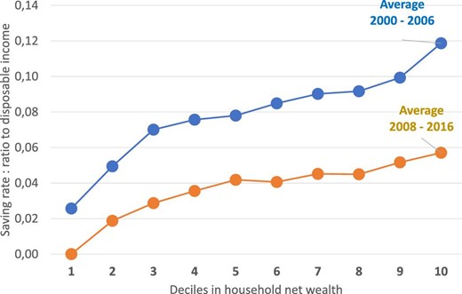
Heterogeneity of saving rates across household wealth groups. The figure shows saving rates by wealth levels estimated from SHIW. The saving rate is defined as the difference between disposable income and consumption as a proportion of disposable income. Saving rates are then re-scaled to account for the proportional difference between the aggregate saving rates estimated in survey data and OECD macroeconomic statistics.
The Joint Distribution of Income and Wealth.
We further investigate whether a growing share of labor or capital incomes is concentrating in the hands of wealthy individuals, and examine the joint distribution of income and wealth to assess the extent to which top wealth holders are also top labor and top capital income earners.
In order to derive the share of total labor income accruing at the top of the wealth distribution, we have linked, at the level of the individual, income from tax data in the year before death to net wealth at death.34 We have repeated this exercise with the wealth observed in 2014, which represents the peak of concentration, and on the wealth observed in 2001, the last year before the temporary elimination of the inheritance tax. Personal Income tax records were analyzed in 2013 and 2000, respectively. We have then built aggregated data matrices, with joint distribution of wealth and labor income for different age groups and genders.
We define labor income as the sum of employment income and self-employment income. We define self-employed income as the sum of professional income, income from sole proprietorship and partnerships. For these categories, it should be taken into account that a part of income is generated from labor, while the remaining part is generated from capital. Capital income is instead defined as the sum of financial capital income (including realized capital gains), lands and buildings income, and residual business income, which we assume are not attributable to labor. However, it is worth noting that some forms of financial income are taxed at source, so they are not captured in personal income tax returns. A precise definition of these income categories can be found in Online Appendix N.2.
In Online Appendix Figure N.2, we show the share of capital income and labor income accruing to the top 1% of the wealth distribution. The concentration of capital income is much greater than the concentration of labor income and even greater than the concentration of personal wealth. However, the dynamics of concentration over time appear relatively stable between 2001 and 2014. While the labor income share for the top 1% of the wealth distribution declined slightly from 2.82% to 2.29%, the share of capital income also increased slightly from 15.5% to 16.1% and does not mimic the sustained rise in wealth concentration at the top. The overall dynamics of top fiscal income shares are mostly driven by what happens to labor income, which accounts for 55% of total reported fiscal income, whereas capital income only accounts for 5% of the total. A similar exercise carried out for France by Garbinti, Goupille-Lebret, and Piketty (2021) shows that the labor income share of wealthy individuals declined substantially over the course of the long run from 1970 onward, moving in the opposite direction to the share of capital income accruing to the top of the wealth distribution. More in line with our evidence, Garbinti, Goupille-Lebret, and Piketty (2021) show much milder dynamics of income shares from 2000 onwards.
We further estimate the probability for top labor earners to belong to the top percentile of the personal wealth distribution. We repeated the exercise for the top 1% and top 0.1% of labor income earners (who reported at least €90,000 and €200,000), and found that between 2001 and 2014 such probability doubled for both groups. It increased from 7.8% to 15.5% for the richest 1% labor income earners and from 20.5% to 54.3% for the top 0.1%. Levels in recent years are similar to what is observed in France (Garbinti, Goupille-Lebret, and Piketty 2021). However, the estimated trend appears to be moving in the opposite direction: In France, the probability of top 1% of labor earners to belong to the top 1% of wealth holders is declining slightly, from 20% in 2000 to 17% in 2012, a negative trend that is much more pronounced if compared with available estimates in 1970, 29%.
On the one hand, the results may indicate that upper wealth ranges may open the doors to top earning positions. On the other hand, consistent with the evidence about raising top income shares over the past decades (Alvaredo and Pisano 2010 and Guzzardi et al. 2022), results may indicate that Italian top labor earners have increasingly higher chances to climb the wealth ladder to the very top (via either higher savings or higher returns to wealth).
However, as remarked in Brandolini et al. (2018), it is important to recall that widening inequalities must be seen in the context of a peculiar macroeconomic setting in which “Italy is the only major advanced country which, in the last two decades, suffered a fall in real household incomes per capita” (p. 5). The documented growing probability for top earners to be at the top of the wealth distribution might therefore have an alternative interpretation: Individuals in the bottom and middle ranks of the income distribution might find it increasingly difficult to climb the wealth ladder. Raising the wealth-to-income ratio (as documented in the introduction) may reflect this growing relative “unaffordability” of wealth for average income earners.
6.3. The Evolution of Wealth over the Life Cycle
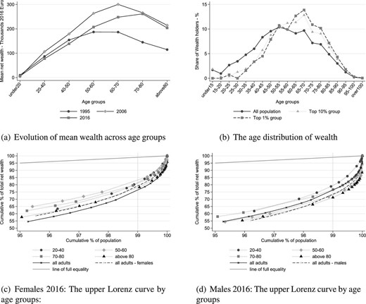
The concentration estimates discussed so far refer to snapshots of the distribution in given years and include wealth and savings accumulated for life cycle purposes. As written in Cowell and Van Kerm (2015), “even if everyone had common wealth accumulation paths over the life cycle, wealth at any point in time would turn out to be unequally distributed when pooling observations of individuals of different age.” Indeed, average wealth does vary considerably across the age distribution; older generations are much richer, as one would expect. In 1995, average wealth peaked at 40–50 years but was less than a third of this amount for the 20–40 age group. Average wealth increased for all ages until 2007 before receding following the Great Recession, in particular for younger groups (Figure 12(a)). However, assessing the average wealth holding between age groups does not sufficiently capture the role of age in determining the extent of wealth concentration.
The life-cycle dimension of wealth distribution and inequality.
To address this concern, we attempt to isolate the effect of age from that of other wealth-generating factors correlated with age, such as education level and birth cohort. To do so, we compute an age-adjusted Gini index that directly isolates the net effect of age on inequality via a multivariate regression model, as suggested in Almas, Havnes, and Mogstad (2012). We apply this method to our tax-based data (where we can only condition on gender) as well as to the survey data (where we can use a richer set of controls such as gender, type of work, sector of work, and education). As shown in Online Appendix S (Figure S.1 and Table S.1), the age-adjusted Gini is found to be at most 0.015 Gini points below the unadjusted one, with no apparent trend effect, suggesting a marginal role of age components in explaining the current wealth distribution.35
Based on Atkinson (1971), we carry out two additional exercises. First, we examine the age distribution of wealth in the overall population and among the wealthiest subgroup. Figure 12(b) shows that individuals of various ages can be found in both the richest groups and the overall population, albeit in different proportions. Second, we analyze the wealth distribution within each age group and compare it with the overall population. Figure 12(c) and (d) depicts the high-end segment of the Lorenz curve for the top 5% of adults in each age/gender group, alongside the overall population. The vertical dotted lines indicate the top 1% in each case. The share of total wealth held by each top 1% group can be derived by subtracting the cumulative percentage of total wealth on the y-axis from 100%, where the vertical line intersects each Lorenz curve. Our results strongly suggest that wealth remains widely concentrated within all age/gender groups, with the shares of total wealth held by the top 1% being roughly similar, regardless of age and gender. Importantly, no group displays significantly lower wealth concentration than the overall population, except for younger males, where wealth appears relatively less concentrated compared with the overall population.
In agreement with Atkinson (1971), we can conclude that “life-cycle factors cannot explain the upper tail of the current distribution of wealth [...] and there are good reasons for believing that there is a high degree of concentration in the distribution of wealth inherited by people over their lives” (pp. 251–252). The relevance of this statement about the residual role of inheritance in driving wealth concentration at the top can be explored with the existing data. We now turn to this important point.
6.4. The Growing Role of Inheritances and its Dwindling Taxation
Intergenerational wealth transfers are crucial economic resources for households that impact long-term wealth concentration dynamics, an area of growing research interest (Nekoei and Seim 2018; Nolan et al. 2020). In this paper, we provide new evidence of the increasing incidence and concentration of bequests and lifetime wealth transfers in Italy. Additionally, we highlight the progressively favorable tax treatment of these transfers for the wealthy.
In low-growth economies, bequests have become more significant for accumulation compared with personal savings, including in Italy (Piketty (2011); Atkinson (2018); Alvaredo, Garbinti, and Piketty (2017)). Our estimates show an approximate doubling of the annual flow of inheritances and gifts from the mid-1990s to the mid-2010s, reaching 14% of national income and 2.3% of personal wealth (Figure 13(a)).36 There is also a concentration of larger bequests in fewer hands, with the richest 1% of decedents increasing their share of total estates by at least 4 percentage points between 1995 and 2016 (from 20% to 23%) (Figure 13(b)). This indirectly suggests a potential concentration of inherited shares. To further explore this, we conduct an exercise assuming equal estate division among two heirs and including lifetime donations in the total estate value based on tax records. This effectively allows us to estimate lifetime wealth transfer concentration measures. Plotting the evidence in Figure 13(b), we show that the share of lifetime transfers received by the richest 1% of heirs increased substantially from 21% to 25%, from 1995 to 2016.37
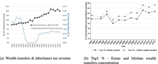
The dynamics of the inheritance and gifts flows, inheritance tax collection, and the concentration of wealth at death and inheritances. Panel (a) shows the value of annual flows of inheritances and gifts inter vivos as share of national income and the value of inheritance tax paid (excluding gift tax) as a share of total annual tax revenue. The effective tax liabilities paid from the inheritance tax forms are reported at year of death. Total annual tax revenue is derived on a year of account basis from official statistics of the Ministry of Economy and Finance. Panel (b) shows the share of total estate value held by the richest 1% of decedents and the share of lifetime wealth transfers received by the richest 1% heirs (the value of lifetime wealth transfers is derived as the sum of total inheritances and total inter vivos gifts; the number of heirs are derived assuming that every decedent have distributed her wealth and donated equally between two heirs). The value of the estates at death and wealth transfers received are adjusted for under-reporting, including among others allowances for the value of tax-exempt assets. The value of estate makes allowance for deceased individuals whose wealth is not reflected in the inheritance tax records (the missing population).
Inheritance patterns are highly relevant for wealth accumulation, even at the top of the distribution. Forbes data on Italian billionaires reveals that six out of the top ten richest individuals inherited their fortunes. Microdata analysis by Nolan et al. (2022) further confirms the significance of wealth transfers among wealthy households across several high income countries. Their study shows that 55% of households in Italy’s top wealth decile reported receiving inheritances or gifts, compared with only 3.4% in the first quartile. The amount received also generally increases as wealth levels rise. While some top 1% households did not receive intergenerational transfers, those who did received considerable amounts. On average, transfers to the top 1% are worth 7 times the overall average transfer value (estimated at €350,000), while for the bottom quartile, this ratio is closer to half. These patterns hold within age groups and reflect the impact of inheritances or gifts on current wealth and position in the wealth distribution.
Despite the growing relevance of inheritance in relation to national income, the receipts from its taxation experienced a notable decrease from 0.14% to 0.06% of tax revenues from the end 1990s to 2016 (Figure 13(a)).38 As argued in Cowell et al. (2018), wealth transfer taxes are crucial to “the long-run distribution of wealth, reducing equilibrium inequality (the ‘predistribution’ effect) by a much larger amount than what is apparent in terms of the immediate impact of the tax (the ‘redistribution’ effect).” Along similar lines, Nekoei and Seim (2018) argue that “inheritance taxation can reduce long-run wealth inequality”, albeit “solely through the taxation of very large inheritances.”
The causes of the reduction in tax revenue are found in the profound changes made to the structure of the estate, inheritance, and gift taxes, including the marked decline of its progressivity over recent decades. As described in Jappelli, Padula, and Pica (2014), the marginal rates of the estate tax ranged from 3% to 27% in the 1990s. In 2000, the inheritance tax was introduced with a unique, proportional tax rate at 4% for transfers received by a spouse or direct relative, which has remained unchanged ever since the tax was reintroduced in 2006. The exemption threshold for similar transfers increased substantially from nearly €125,000 between 1995 and 1999, to nearly €175,000 until 2000, and then to €1 million from 2006 onward.
Between 1995 and 1999, 70% of the estates valued above €300,000 were subject to taxation. Under the tax regime in place since October 2006, as highlighted in Figure 14(a), only 30% of estates valued between €2.5 million and €6 million, and less than 80% of the richest estates (€10 million and above) were subject to taxation, on average. At the same time, the share of estates between zero and €20,000 subject to taxation increased from 1.6% in the pre-2000 tax regime to 14% on average in the current tax regime. Many small estates are now subject to taxation due to the fact that the exemption threshold was cancelled for wealth transfers beyond the fourth degree of kinship. Even small inheritances are, therefore, subject to taxation if received from donors outside the more direct family sphere. As a result, the share of total estates that are now subject to taxation is just above 10%, compared to 8% in the 1990s. Furthermore, conditionally on being taxed, the richest estates now have a substantially lower tax bill. Prior to 2000, the richest estates (€10 million and above) paid the equivalent of 6.3% of the estate in taxes, with considerable variance around this value.39
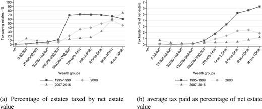
The decline of the tax burden on the wealthy. Panel (a) shows the % of estates subject to inheritance tax. Panel (b) shows the average tax burden by net estate ranges. Following the evolution of major reforms in the tax structure in 2000 and 2006, we compare the average values of the above-mentioned indicators across three main periods: 1995–1999, 2000, and 2007–2016. The 2001–2006 period is excluded as the inheritance tax was abolished in Italy during this period. The average tax burden is estimated based on the tax liability associated to each estate, computed as the sum of the tax applied on the global value of the estate, when applicable (i.e., before 2000), and on the share of the estate inherited by the heirs.
As shown in Figure 14(b), the average tax bill on the same estate has, since 2006, dropped to 1.2% of the estate value. This is not too dissimilar from the average tax bill of 0.7% associated with very small estates (between 0 and €20,000). Therefore, under the current regime, a much smaller share of large estates are subject to taxation, the average tax rate for the largest estates has dropped by 80%, and the progressive structure of the inheritance tax—relative to the estate value—no longer exists. This does not necessarily mean that the major changes to the inheritance tax in Italy since 2000 have directly determined the increase in wealth concentration in the same period; nevertheless, it may well play a more substantial role in the long-run.
7. Robustness Analysis
7.1. Alternative Mortality Rates
Older people, as expected, have higher mortality rates than younger ones. Similarly, males tend to have a shorter life span than females. However, demographic factors are not the only ones influencing mortality. Socio-economic conditions such as marital status, geographical location, education, and income or wealth matter too. In particular, failure to appropriately account for mortality heterogeneity may result in biased estimates of the distribution of wealth, a point already highlighted in earlier work (Atkinson and Harrison 1978). Nevertheless, this intuition is not always correct, because the underlying distribution of estates also plays a role, as explained in Alvaredo, Atkinson, and Morelli (2018).
To check for robustness, we make use of the linking of the mortality records to the education levels produced by ISTAT for 2012, and for age groups between 25 and 90. A distinction is drawn between four education groups: no education or elementary school; middle school; high school; and college degree or higher.40 The life expectancy of a 25 year-old with no education or with elementary school education is 4 years lower, on average, than that of an individual holding a college degree or higher. For males specifically, the difference in life expectancy is 5 years higher. Online Appendix Table O.1 shows that, in 2012, the mortality rate for 40 year-old males was on average 0.16%. This mortality rate drops by more than half for a male in the same age group that holds a college degree or higher. By contrast, the mortality rate is more than twice the average (206%) for those who only received elementary education.41
In seeking to establish whether and how steeper mortality multipliers change wealth concentration estimates, we assume that individuals with assets above €1 million have a relative longevity advantage—in relation to the overall population with the same demographic characteristics—similar to those in the highest education class. Individuals with wealth below €50,000 have been assumed to have the same mortality rate to those who hold at most elementary education. Finally, individuals occupying intermediate wealth ranges, namely between €50,000 and €300,000 and up to €1 million, are assumed to have mortality patterns similar to those with middle school and high school education, respectively. This type of adjustment is imperfect and the information on mortality rates adjusted by education is only available for 2012; the same relative adjustments have been applied to the remaining years in our sample. The direction of change is as expected, an increase in top shares, but the difference with the benchmark series at the top is small (for a more detailed discussion on the nature of these adjustments and their implications for top wealth shares; see Alvaredo, Atkinson, and Morelli 2018; Berman and Morelli 2022).
A further confirmation that the results are robust to the use of more refined mortality multipliers is the use of tabulations containing finer disaggregation by age bracket and geographical location. Multipliers in 1995 were lower in the north of the country compared with the south and the islands. By 2016, it was the opposite. Theoretically, not accounting for such heterogeneity may create a downward bias on the increasing trend in wealth concentration, given that the northern areas are the wealthiest. The concentration series, excluding any imputations, are robust in the presence of such refinements (see Figure O.1 in the Online Appendix).
7.2. The Inclusion of Durables
The exclusion of durables from the national balance sheets (accounting for 8% of total wealth identified in the 2016 SHIW data) would likely be felt more strongly in the bottom parts of the distribution. As shown in Figure 15, including durables would, in fact, reduce the top shares marginally, but would increase the share of the bottom 50% by a non-trivial 1–2 percentage points.
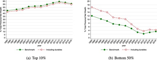
Top 10% and Bottom 50% shares in total wealth: including and excluding durables. The value of durables is imputed to the gender, age, location, and wealth levels as reported in the survey data.
7.3. The Role of Imputations
For the benchmark series, we make the following imputations: (i) we first multiply up the estate distribution using mortality multipliers; (ii) we then append an estimate of the wealth of the missing population based on household survey data; and finally, (iii) we distribute the remaining wealth gap with respect to the NA, according to the relative distribution of asset classes in the identified wealth from tax records complemented by that of the missing population from survey data.
One must wonder to what extent the benchmark estimates are driven by specific imputation choices in steps (ii) and (iii). To address this concern, we discuss two alternative imputation scenarios. First, we derive a series that imputes the wealth gap by relying exclusively on the identified asset distribution based on tax records; second, we derive a series where step (ii) is based exclusively on values reported in the household survey data, rather than relying on adjusted values to account for underreporting.42 Both approaches attach more weight to wealth reported in the tax records, which is on average more concentrated than what would appear if one only considered smaller wealth holdings that go unnoticed by the tax authority. Hence, the alternative set of imputations, when compared with our benchmark series, generally suggest a higher wealth concentration at the top and a lower share for the bottom 50% of the population (details are given in Online Appendix O.3).
Wealth Concentration with no Imputations.
Most importantly, we also estimate wealth concentration without resorting to imputations (i.e., entirely bypassing step (iii) above). The derivation of unadjusted wealth concentration statistics enhances our understanding of the series and their comparability across countries, given this was the dominant procedure in the literature until recently. Estimates for the UK in Atkinson and Harrison (1978) and Alvaredo, Atkinson, and Morelli (2018), for instance, followed this path. Importantly, this was done using both internal and external wealth totals. Typically, researchers use external data (e.g. NA) on total wealth that bear no relation to tax data. However, when the population coverage of inheritance tax records is particularly high (as in the cases of Italy or the UK), one can also rely on the multiplied-up estates as well as the estimated wealth of the missing population to derive an internal measure for total wealth.
Figure 16(a) and (b) illustrates these results. The series for the top 1% share based on both external and internal totals without imputations point to a more moderate increase in inequality over the past decades (the top 1% increased by 1 percentage point from 1995 to 2016 and by 5 to 6 percentage points from 1995 to 2014). 43 The evolution of the top 1% share based on internal totals and no imputations is also compared with that of other countries available from existing literature. Both levels of wealth concentration in Italy as well as the direction of their trends appear very much in line with available comparable estimates for the UK, Norway, Finland, Sweden, Spain, and the Netherlands.
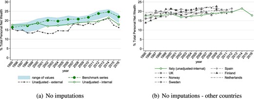
Top 1% share without imputations. Panel (a) compares the benchmark series of the wealth share of top 1%, consistent with the NA, with two series derived without resorting to any imputations of missing wealth. The two series reflect different strategies to estimate an appropriate wealth total (i.e., the denominator). On the one hand, we subtract tax-exempt assets from the NA total (external total). On the other hand, we estimate the wealth of the missing population and add it to the identified wealth obtained through the re-scaling the inheritance tax records with mortality multipliers (internal total). Panel (b) compares the “internal total” series to the evolution of wealth concentration in other countries. The UK series is taken from Alvaredo, Atkinson, and Morelli (2018) and is directly comparable to the Italian one (e.g., both series refer to individual adults and are derived from the inheritance tax data using an internal total and no imputations). Figures for Finland, the Netherlands, Norway, Sweden estimated by Roine and Waldenström (2015) are from wealth tax tabulations and refer to household units (with the exception of Finland, where data refer to individual adults). Data for Spain refer to individual adults and are taken from Alvaredo and Saez (2009) from wealth tax data.
This suggests that the imputation procedures of unobserved wealth can play an important role in generating cross-country heterogeneity in the levels and trends of wealth concentration, and as such should be carefully assessed and understood.44
The role of imputations appears stronger particularly in those years where the underlying inheritance tax data are less complete. For instance, between 2001 and 2006, the inheritance tax was abolished and the unadjusted data are only informative about housing wealth holdings. Similarly, in 2014, the tax legislation increased the non-filing threshold from €25,823 to €100,000. This has likely worsened the quality of unadjusted information from which to derive compelling wealth distributional estimates. Indeed, as documented in Online Appendix H, the number of unidentified adults increases by 1.5 million from 2012 to 2014, and whereas the total net wealth identified from the inheritance tax records amounted to 85% of total personal net wealth from macroeconomic statistics, this ratio dropped to 70% by 2016 (see Online Appendix G).
Hence, we believe our benchmark series, with the imputation of missing wealth, represents a more convincing representation of the actual dynamics and levels of wealth concentration in Italy over recent decades.
Final Remarks
“Statistics on wealth distribution,” writes Atkinson (1978), “play ‘a key political role’ and they are as sensitive an issue as the balance of payments or unemployment figures. This means that it is all the more important that they should be firmly based. We should examine critically the evidence and the assumptions underlying it.” With these principles in mind, this paper makes contributions along three dimensions: methodological, empirical, and on implications for future research.
This paper estimates new series of wealth inequality in Italy between 1995 and 2016, a period of substantial economic turbulence and structural reforms for the national economy. The work uses, for the first time, the full set of inheritance tax returns with substantial coverage of the population. This high-quality data also provides a more convincing coverage of the upper end of the wealth distribution compared with existing household surveys. Our benchmark estimates fully redistribute the wealth of the household sector found in the NA. As this involves a number of controversial decisions, we have adopted a multi-series approach, that is, one that allows for the possibility of comparing information provided by different and competing data sources. A series without imputations is also estimated. We firmly believe that, given the current, imperfect state of data on the distribution of assets and liabilities, such an approach is preferable to the alternative option of looking at a unique series.
Our main results suggest a substantial increase in wealth concentration and wealth inequality, and a dramatic decline of wealth shares held by the bottom groups of the adult population. Over the past two decades, Italian wealth distribution has become substantially more unequal. The 2008–2009 financial crisis, as well as the ensuing double-dip economic recession and European debt crisis, which peaked between 2010 and 2012, appear to have markedly accelerated the process, with the bottom 50% of the adult population now holding only 3% of total wealth, while the richest 0.1% hold more than 10%. In the 2000s, these two groups held a similar share of total wealth, around 7%, before starting to diverge. The evidence collected suggests that wealth growth has been predominantly driven by the volume of savings. Although the changes in asset prices are not the main factors explaining the increase in wealth concentration, changes in equity prices account for a large share of wealth growth above the 99th percentile. We also show that age and life-cycle factors play a marginal role in explaining wealth concentration levels and dynamics. Finally, we provide evidence of the growing concentration of inheritances at the top, as well as the decreasing tax burden on wealthy inheritors.
Growing wealth disparities in this scenario appear concerning on several grounds. First, rising wealth inequality may be coupled with growing financial vulnerability and insecurity for a vast number of adult individuals who have limited private financial resources to cushion adverse circumstances. Second, growing inequalities of wealth holdings can have corrosive effects on equality of opportunity when they turn into persistent disparities across generations. Available, comparable cross-country measures suggest that Italy (as well as the US) is one of the countries where offsprings’ earnings are the most dependent on those of their parents, implying low intergenerational mobility across generations (for a discussion see Corak 2013; Acciari, Polo, and Violante 2022; Bloise 2018; Cannari and D’Alessio 2018a).
Despite the empirical contribution of this paper, many data limitations remain, and it is imperative to invest in official statistics to measure direct and indirect wealth holding and to shed further light on the main determinants of large fortunes and wealth concentration. Three main steps can be taken to improve data on wealth distribution in Italy.
First, the stock of asset holdings may be indirectly estimated through the observation of their resulting yields via capitalization methods. The fact that this method is currently not easily implementable in Italy due to the existing taxation structure (most capital incomes are taxed at source and are not reported in tax files) should not be understood as an absolute impediment to producing the statistical information behind those flows.
Second, we have shown that the creation of a comprehensive asset registry would imply substantial progress. The existing real estate registry should be made accessible for research purposes. Since 2011, a financial assets registry is already a concrete reality as financial institutions share data on individual financial wealth holdings with the Revenue Agency. However, this registry remains inaccessible.45
Third, a renovated household survey, that over-samples wealthy households and links respondents to administrative registers, could improve knowledge of wealth distribution by making it more accurate. This includes better data on the poorer segments of the wealth distribution to gain a more complete view of households’ financial vulnerability. The COVID-19 pandemic highlighted the importance of personal liquid assets to accommodate large income shocks for a sustained period of time. The focus on households as the unit of analysis remains helpful for understanding the welfare implications of wealth distribution. The use of household survey data also remains crucial to analyzing the complex interactions between the need to accumulate private wealth and the provision of public goods, services, and social security benefits.
Notes
The editor in charge of this paper was Nicola Pavoni.
Acknowledgments
We are grateful to the Department of Finance of the Italian Ministry of Economy and Finance for providing technical support and access to some of the data. The views expressed in the paper are the authors’ responsibility only. We are grateful to many scholars for fruitful discussions and feedback at different stages: Charlotte Bartels, Michele Bavaro, Yonatan Berman, Giovanni D’Alessio, Riccardo De Bonis, Carolyn Fisher, Giacomo Gabbuti, Janet Gornick, Elena Granaglia, Arthur Kennickell, Clara Martinez-Toledano, Marco Ranaldi, Giacomo Rella, Alfonso Rosolia, Simone Tedeschi, Giovanni Vecchi, and Gabriel Zucman. We thank Demetrio Guzzardi for excellent research assistance as well as Francesco Bloise, Pietro Geuna, Anna Grimaldi, and Ercio Muñoz for additional support. We also thank four referees, the co-editor Nicola Pavoni, and a referee from the Italian Department of Finance Working Papers. We acknowledge financial support from the Cazzavillan Fellowship at the University of Venice Ca’Foscari (SM), the European Research Council (FA, Grant 856455), the Agence Nationale de la Recherche (FA, Grant 17-EURE-0001), as well as the generous support over many years by the Institute for New Economic Thinking-INET (FA). Salvatore Morelli acknowledges support during visiting periods from the Fondazione Lelio e Lisli Basso, the Department of Social Policy and Intervention, and Nuffield College at the University of Oxford.
Footnotes
See wid.world.
There are at least six potential sources of evidence to study the distribution of personal wealth: (i) administrative data on the wealth of the living derived from annual wealth taxes; (ii) administrative data on investment income, capitalized to yield estimates of underlying wealth; (iii) administrative data on individual estates at death, multiplied up to yield estimates of the wealth of the living; (iv) household surveys; (v) lists of large wealth holders, such as the Forbes list; and (vi) population censuses.
This is the result of the combination of the very high homeownership rate with a key administrative feature of the tax, which is strictly connected to the upkeep of the cadastral (real estate) register: all inheritances involving the transfer of real estate property are obliged to file a return, even when no tax is due (and even during the period when the inheritance tax itself was abolished between 2001 and 2006).
The cumulative capital gains in housing wealth are relatively small given that house prices were increasing substantially until 2008 and then declined thereafter. Despite the particular relevance of housing assets across the distribution, this may explain why the results for Italy are somewhat different from those found in recent research on France, Germany, Spain, the UK, the US, and China (see Kuhn, Schularick, and Steins (2020) and Bauluz, Novokmet, and Schularick (2022)).
The aggregate value in 2020 was €559.8 billion according to the “consumer durables” supplementary series estimated in the national balance sheet for the household sector and the non-profit sector serving households. In SHIW data, the aggregate value of means of transportation and other durables (furniture, furnishings, and appliances) owned by households was 4% of personal wealth in 2016, equal to €366 billion in 2016.
Using data from Australia, Longmuir (2021) shows that adding an estimate of the present value of social security pension wealth to the standard definition of net worth has “an equalizing effect, as the Gini index in 2018 reduces from 0.66 for net worth to 0.571 for augmented wealth.” Findings of a “ sharp fall of wealth inequality’’ when public pension wealth is included are also highlighted in the work by Cowell et al. (2017) for 13 European countries.
This form of “compulsory savings” is called Trattamento di Fine Rapporto, TFR.
Unincorporated businesses fall into two main categories. As discussed in Rodano and Signorini (2008), the ESA95 includes the so-called “quasi-corporations” in the non-financial corporations sector. “Quasi-corporations are defined as organizations not having independent legal status that keep a full set of accounts, and whose economic and financial behavior is different from that of their owners [...] In Italy, the operational definition of nonfinancial quasi-corporations includes all firms that take the more formal types of unlimited liability partnerships (società in nome collettivo, società in accomandita semplice) regardless of size; it also includes simpler partnerships (società semplici, società di fatto) and sole proprietorships (ditte individuali), provided they have more than five employees [...] The rest (i.e., simple partnerships and sole proprietorships with up to five employees) are to be recorded in the producer households sub-sector” (p. 150).
See Online Appendix A.4 for details on the value of business shares and equities in the financial and macroeconomic accounts.
Only the net value of assets located in Italy is included in the tax base in the case of a person not deemed domiciled in Italy for tax purposes.
In the presence of a disabled heir, the tax-exempt threshold is €1.5 million.
In 2000 and 2001, the gift tax rates were 1 percentage point lower than the inheritance tax rates.
It is not yet clear if this provision is still in force, as the Supreme Court issued non-unanimous judgments on this between 2016 and 2019. A system purely based on lifetime capital receipts, irrespective of the identity of the donor, would be more effective in reducing tax avoidance. Currently, a single heir can receive different inheritances and still pay zero taxes as long as each share is below the exemption threshold. It is also important to note that in case the coacervo is definitively foreclosed by developing jurisprudence, inheritance tax avoidance schemes through inter vivos gifts will be easier.
The rate dropped to 61% in 2015 also due to unexpectedly high mortality rates that year. The total number of deaths in 2015 amounted to 648,000, 40,000 above the average number of deaths in 2012–2016. The relative (small) decline of the rate after 2014 may also be due to a change in legislation (passed at the end of 2014) that increased the non-filing threshold from 50,000,000 Italian Lira (i.e., €25,823) to €100,000 (the threshold defining the net value above which the filing is required for those estates without any real estate properties or rights).
In October 1999, the first tax bracket was eliminated and the tax exemption threshold increased from €125,000 to €175,000.
Tax returns are submitted to the tax office in the province where the deceased held residence. Until 2003, the time limit was 6 months. The latest data update in this paper was obtained in May 2020. A set of 2,600 tax returns presented in 2018 with the new electronic form, but related to deaths occurred in 2016, were included in the data. In principle, there could be a very small number of tax returns submitted or revised even 10 or 20 years after death as more precise information about the estate comes to light, but these amendments are not taken into account in the statistics. Every year-specific database becomes consolidated for our purposes if 2 years have passed since the year of death.
For instance, financial institutions need to certify the balances of all accounts; the cadastral office certifies the cadastral value of buildings, land, or dwellings; a certified copy of the most recent balance sheets needs to be attached to prove the book value of any personal business; and the official certification of ownership of listed corporate stocks should also be provided. Similarly, all the expenses and liabilities that are reported for deduction purposes need to be appropriately documented.
We also make use of more refined age decomposition based on 23 five-year age groups for a subset of years, namely for 1995 and for the post-2012 period. Note also that a negligible number of observations do not report the gender or age of the decedent. These account for “ gender not stated” or “ age not stated”, respectively.
Starting from 2017 only, the paper module for inheritance tax returns has gradually been replaced by an electronic form that includes a considerable amount of additional detail about the composition of estates.
Online Appendix D provides a description of the mortality data, and a more detailed discussion about how mortality multipliers affect the age distribution of wealth holdings.
The transformation from household to personal wealth is described in Online Appendix K, and follows D’Alessio 2018.
Refer to Online Appendices Figures F.1(b) and H.1(b). Online Appendix Figure F.2(a) shows that the coverage rates are lower for younger age groups and very low for those aged 20 or less who are more likely to have zero wealth holdings
The underestimation of market values could be particularly salient for older buildings whose value has not been updated for many decades. The sell-up value is reported only for those buildings under construction or for those for which no cadastral rent has yet been attributed.
There are now 134 countries whose tax authorities have an “adequate” exchange of information with Italy. As a result, these countries are included in the so-called “white list,” required to access to more favorable tax treatment.
The tax exemption status is valid on the condition that the business is run and the control share is maintained for at least 5 years from the wealth transfer at death. Nonetheless, and similarly to what happens to any real estate rights, the value of business assets has to be reported in the inheritance tax returns and will be deducted from the final liability. The remaining exempted assets are generally not reported on tax records. It is also worth mentioning that inherited or donated assets of any kind may be fully exempted if the recipient belongs to one of these categories: religious entities, NGOs, political parties, state, regional or local authorities, and research institutions.
We include 100% of government securities during the years where the estate, gift, and inheritance tax was not in place (e.g. the period included between October 2001 and October 2006).
This result follows from Atkinson et al. (1970) under the simple condition that the inequality indicator considered is consistent with the Pigou–Dalton principle of transfers. Such a principle requires, loosely speaking, that any transfer from the rich to the poor in which the rich remain richer than the poor would lead to a decrease in inequality.
The same share was assumed in Johannesen and Zucman (2014) and appears consistent with García Luna and Hardy (2019) who found that at the end of March 2019, households (including non-profit institutions serving households) accounted for 51% of Swiss banks’ cross-border liabilities. In the same work, when considering all the countries in the sample, households account for only 14% of banks’ cross-border liabilities.
Incidentally, this figure is very similar to the 2007 value reported for Italy in Alstadsæter, Johannesen, and Zucman (2018), €191.3 billion, or $262.2 billion USD.
It is worth remembering, as pointed out in Deaton (2005), that the absence of the rich from surveys does not necessarily imply that measured inequality is biased downwards.
The financial and business asset category is very coarse and the composition of assets within this category can vary a great deal across the distribution. For instance, it may well be that the bottom and middle part of the distribution mostly hold pension and life insurance assets or safer government bonds, whereas riskier shares in public and private companies and mutual funds may be the prevalent financial investment at the very top of the distribution. To account for such heterogeneity in the composition of financial assets across the distribution, we consider −30% the share price index change for the bottom 90% of the distribution and +30% the share price index change for the groups above the 99th percentile. This adjustment means that the share price index increases between 1995 and 2016 would change from 64%, as reported in the OECD data, to 45% for the bottom 90% and to 83% for the wealth groups within the top percentile. Data on asset prices from the OECD are reported in Online Appendix Table N.4.
The periods are not symmetrical given the data structure at hand. First, our data series begins in 1995. Moreover, taking 2000–2008 as one of the period of reference avoids relying on wealth composition information during years in which the quality of data is diminished (the inheritance tax was abolished between 2001 and 2006). Note also that the results are robust to the use of cumulative price changes between 1995 and 2008 and between 1995 and 2016 without considering sub-periods in the analysis. The main difference being that the exclusion of sub-periods would slightly overestimate the role of capital gains for financial assets.
We have then applied mortality multipliers to derive the joint distribution of income and wealth for the living. Similarly, we have derived the estimated market valuation of real estates correcting the reported cadastral values. See Section 3.3 for a detailed description of both passages.
The adjustment procedure proposed by Almas, Havnes, and Mogstad (2012) relies on calculations of the Gini coefficients without negatives and substituting all zeros with 1. Although the method can isolate the effect of age components, this makes the method less appealing for estimating the actual levels of wealth inequality given the substantial role played by zeroes and negative values in the distribution of wealth.
These estimates are very closely aligned to those shown in Acciari and Morelli (2022), relying mostly on declared information on tax statistics, with aggregate and proportional corrections for under-reporting of wealth. Yet the estimates presented in this paper rely on the benchmark wealth distribution of the entire population reconciled with the national households balance sheet. Total wealth holdings are classified by gender, location, and age groups and each cell is multiplied by the relevant mortality rate (as estimated by ISTAT). This exercise represents a reverse engineering of the mortality multiplier method, estimating the entire deceased population and its wealth holdings every year. The advantage of this approach is the derivation of a full distribution of the estates at death, including implied adjustments to their wealth reported on the tax records as well as an allowance for the wealth of non-filers. A similar approach was applied by Cannari and D’Alessio (2008) to simulate inheritance receipts by applying mortality tables to the reported wealth in the Survey of Income and Wealth. In this case, the total value of inheritance flows as a share of total net worth is substantially lower and increased much more moderately over time, from 0.99% in 1995 to 1.52% in 2016. The estimated series of total annual flows of gifts cannot be estimated with this method and has instead been taken from Acciari and Morelli (2022).
Note that the adjustments for missing wealth would rely on a poor set of information in the years when the inheritance tax was cancelled (2001–2006), as the reporting of assets other than real estates was compromised. For this reason, the levels of adjusted concentration estimates in the years 2002, 2004, and 2006 are proportionally linked to the unadjusted concentration figures in 2001 and 2008. More detailed information about the distribution of estate at death and the lifetime wealth transfers are shown in Online Appendix P.
The total revenue generated from the inheritance tax associated with individuals who died in 2016 was €400 million. The official figure of the Ministry of Economy and Finance for the inheritance tax revenue, measured at the year of account and not at year of death, is €558 million for 2016. An additional €183 million came from the gift tax.
As shown in the Online Appendix I, the average tax rate for estates above €10 million could be higher than 20% of the estate value or as low as zero. Given the existence of a large category of tax-exempt assets, the effective tax rates depend substantially on the composition of the estate.
The ISTAT original classification is the following: “Nessun titolo o Licenza elementare”; “Licenza media inferiore”; “Licenza media superiore;” and “Laurea o titolo superiore.” Two additional categories are dropped as redundant: “Nessun titolo o licenza elementare o licenza media inferiore;” and “Licenza elementare o licenza media inferiore.”
This mortality rate gradient by education groups is similar to that used by Kopczuk and Saez (2004) for the US.
As mentioned earlier in the paper, to account for the underreporting of assets in the household survey data, we proportionally adjust non-housing asset values using the ratio of total value between the NA and the SHIW, asset class by asset class.
Online Appendix O.4 provides more evidence about different wealth groups. For instance, evidence for the top 10% wealth share shows a much more pronounced increase in wealth concentration over the same period, from 44.3% in 1995 to 48.5% in 2016. Notice also that the external total series without imputations can be derived on a yearly basis, as it does not require any information from household survey data to be estimated.
Notice also that the evidence provided by our unadjusted series shows that the level of wealth concentration is more aligned with that obtained using comparable estimates derived from the SHIW. Yet the level of wealth concentration remains higher with a more pronounced positive trend (see Figure O.6 in the Online Appendix).
According to Decree Law 06/12/2011, n. 201, article 11, such data can only be used for tax evasion risk analysis and for other institutional activities of the public authorities.
