


Abstract
To assess the life-cycle welfare effects of pension reforms, we provide a dynamic stochastic model of saving, portfolio choice, and retirement featuring a rich characterisation of the pension system. Relying on the exogenous variation from a sequence of Italian pension reforms, we identify and estimate the model, which is then used to draw implications of alternative pension policies. The validated model predicts substantial social security wealth effects on retirement, with the offset between public pension wealth and private savings softened when households can adjust their retirement decisions. We further find important distributional effects of pension reforms, with households’ welfare decreasing more the later in the working life they face the reform. Our findings have implications for the design of pension policies and the support they might generate.
A set of Teaching Slides to accompany this article is available online as Supplementary Data.
1. Introduction
The population aging, and the related challenges to the pay-as-you-go social security systems, caused profound changes to the pension legislation in several OECD economies. While there is wide between-countries variation in the extent, the speed and the timing of these changes, a common trait has been the occurrence of heated policy debates over alternative interventions in social security systems. Most often, these debates lack the discipline of an operational economic model to understand the effects of pension legislation changes on households decisions and welfare. This is especially important since the literature remains divided on the answer to two long-standing and related questions at the root of the policy debate: (i) how public pensions crowd-out private savings and (ii) how social security wealth affects retirement decisions. On one hand, while social security wealth is a perfect substitute for private savings in a canonical life-cycle model with fixed retirement, the effect of public pension wealth on private wealth is theoretically ambiguous when retirement is endogenous (Feldstein 1974). On the other hand, while the vast empirical literature on the offset between social security and private wealth has been inconclusive (see, e.g. Lachowska and Myck 2018 for a recent review), there is little evidence on the effect of social security wealth on retirement (Blundell, French, and Tetlow 2016b). Further, analysing the welfare effects of pension reforms is a difficult task due to the complexity of pension rules and economic environment in which individuals take decisions. Understanding these effects is crucial to the design of pension reforms, most importantly before the reform takes place. We exploit quasi-experimental variation from pension reforms to validate a life-cycle framework to study the effects of alternative pension policies on households’ saving and retirement decisions and, ultimately, their welfare.
A body of economic research focuses on the evaluation of a social program before its actual introduction, as part of the problem of studying the effect of policy changes without the availability of ex-post information. The ex-ante evaluation of social programs sheds light into the understanding of which range of effects to expect from the introduction of alternative policy changes (Todd and Wolpin 2006b; Heckman 2010). It can then provide a number of useful prescriptions to the policy makers. Todd and Wolpin (2006a) and Attanasio, Meghir, and Santiago (2012) follow this approach to develop and estimate two different dynamic models of education choices to study the impact of the PROGRESA program on children’s schooling attendance; Blundell et al. (2016a) rely on tax and benefit reforms in the United Kingdom to estimate a dynamic model of employment, human capital accumulation, and savings and to analyze the effects of welfare policies.
In this paper, we also propose an ex-ante policy evaluation exercise and exploit the—arguably exogenous—variation induced by pension reforms. We focus on Italy, an interesting case because of the dramatic changes to the pension legislation occurred in the early 90’s. For younger generations of workers, who entered the labor market after 1978, the contribution model replaced the earnings model for the computation of pension benefits. The earnings model was kept for the older generation of workers, but the generosity of the public sector formula was reduced. These reforms also introduced flexible retirement age, with incentives for workers to postpone retirement, again drawing a line between younger and older workers. The extent of the changes and the policies discontinuity among workers made Italy an almost ideal “laboratory” to study the impact of pension policies on households behavior. Miniaci and Weber (1999), Attanasio and Brugiavini (2003), Bottazzi, Jappelli, and Padula (2006) and Bottazzi, Jappelli, and Padula (2011) use the Italian laboratory to investigate the effect of these pension reforms on households decisions, looking at consumption, saving, and portfolio choices. Our exercise shares with theirs the same quasi-experimental variation, but differs in exploiting such variation to inform an economic model about the most relevant channels through which pension reforms affect household behavior.
The reduced form effects, estimated exploiting a difference in differences (DiD) identification strategy, suggest substantial responses of households to the pension reforms in terms of discretionary wealth accumulation, participation in the financial markets as well as expectations about future retirement age. These estimates represent the first stage in our estimation exercise. In the second stage, we develop and estimate a dynamic stochastic life-cycle model in which households maximize expected lifetime utility choosing consumption, the allocation of wealth to risky assets, and the age of retirement, while facing uncertainty with respect to income, returns from the risky assets, and mortality. The model features a rich characterisation of the Italian pension system before and after the pension reforms, explicitly incorporating the transition from a defined benefits (DBs) to a notionally defined contributions (NDCs) scheme, which has been brought forward as a prominent option of social security reform (Lindbeck and Persson 2003; Börsch-Supan 2005).1 The model developed in this paper can be used to draw implications that extend beyond any specific institutional context.
To estimate the model, we target the first stage impacts of the reforms on discretionary wealth and participation in the financial markets. The structural approach carefully replicates the institutional setting, allowing for (ex-ante) heterogeneity with respect to the sector of employment, which in turn determines the treatment status under the pension reforms. Years of work history in 1995 depend on year-of-birth. We consider six year-of-birth cohorts of households, with variation in cohort membership implying variation in the treatment status. Since we match the model-driven impacts of major pension reforms to their data-driven counterpart, we provide an arguably credible tool to conduct ex-ante policy analysis. In particular, adopting a structural approach allows us to overcome two limitations inherently associated with the usage of a standard DiD strategy to study the effect of pension reforms: (i) the concerns about the credibility of the identifying assumptions, upon which the DiD strategy relies (parallel trend and linearity of the functional form); (ii) even when the empirical effects are credibly identified, they are not informative on the offset between public pension and discretionary wealth, the long-run saving and actual retirement behavior of households, the welfare implications of these reforms nor the consequences of alternative pension policies. By using an indirect inference approach to the structural estimation with a DiD regression as auxiliary model, we obtain unbiased estimates of the structural parameters irrespective of the unbiasedness of the DiD estimate as the causal effect of the reform.
The estimated model, with reasonable values for the structural parameters, matches key pre-intervention statistics and the average effects of the pension reforms estimated from actual data exploiting the DiD identification strategy. By validating a life-cycle model with the reduced form effects of pension reforms, we contribute to the vast literature (pioneered by Deaton 1991; Carroll 1997; Attanasio et al. 1999; Gourinchas and Parker 2002) that studies intertemporal choices of consumption and savings. This literature typically estimate the structural parameters targeting the observed behavior of households over some windows of their life-cycle, with identification mostly relying on the age profiles of consumption (e.g. Gourinchas and Parker 2002), income, or wealth (e.g. French 2005). To the best of our knowledge, we are the first to estimate the structural model exploiting quasi-experimental variation from pension reforms for identification.2 Using the method proposed by Andrews, Gentzkow, and Shapiro (2017), we show that the empirical DiD effects of the reform are important for the estimation of the structural parameters. Matching the empirical effects with the model-driven counterparts allows us to address concerns over structural models failing to replicate the effects of actual policy changes (Heckman 2010). Further, we are the first to estimate a fully fledged life-cycle model of savings, portfolio allocation, and retirement for the Italian economy. In this respect, the model extends previous models of portfolio choice, typically assuming an exogenous retirement date (see Gomes, Haliassos, and Ramadorai 2021), and models of retirement, where households save in one risk-free asset (see Blundell, French, and Tetlow 2016b). We add to the literature that studies retirement decisions in life-cycle models (see, e.g. French 2005; Blau 2008; French and Jones 2011; Haan and Prowse 2014) also by explicitly introducing the dynamic incentives individuals face to postpone retirement under the NDC pension system.
Most importantly, the structural approach provides important novel insights about the consequences of the pension reforms, with implications beyond the specific reforms exploited in this paper for model validation. First, we shed further light on the displacement effect between public pension and private wealth, in that contributing to the literature starting from Feldstein (1974). Although recent studies in this literature rely on credible identification strategies, some report high offset (above 0.5) (Attanasio and Brugiavini 2003; Attanasio and Rohwedder 2003; Bottazzi, Jappelli, and Padula 2006; Aguila 2011; Alessie, Angelini, and van Santen 2013), while others find low or no offset (Feng et al. 2011; Chetty et al. 2014; Lachowska and Myck 2018). Our results show an offset between social security and private wealth of about 0.65, holding retirement age constant. Allowing for flexible retirement, the model-predicted offset is about 0.55, indicating that neglecting the retirement response to changes in public pension wealth can downward bias its estimate. Second, and related, the model predicts substantial social security wealth effects on retirement: following a 10% decrease in the pension benefits they would receive for a given age of retirement, households postpone retirement by around 0.5 years on average. To the best of our knowledge, this is the first paper that provides a validated structural estimate for the social security wealth effect on retirement exploiting variation in benefit generosity. This finding complements previous empirical evidence on the effects of social security financial incentives on labor supply (Börsch-Supan 2000; Gruber and Orszag 2003; Mastrobuoni 2009; Engels et al. 2017). Manoli and Weber (2016) provide non-parametric evidence of substantial retirement decisions response to financial incentives using data from Austria. Third, the model shows older households in working age experience substantially larger welfare losses for the same variation in pension rules. It thus provides a quantification and rationalization of “life-cycle” welfare effects of pension reforms, so far overlooked in the literature. Households would be willing to pay around 2.4% of annual consumption on average to face the reform 10 years earlier in their life-cycle. We show our main findings are robust to modifying the set of auxiliary parameters/moments or the structural model specification. Finally, we use the estimated model to show how two alternative pension policies, an increase in the early retirement age and a reduction in benefit generosity, can have different implications in terms of individuals’ retirement and saving responses across the wealth distribution.
The rest of the work is organized as follows. Section 2 presents the main features of the institutional framework, some stylized facts from the data and the empirical strategy to estimate the reduced form effects of the pension reform. In Section 3, we present the dynamic life-cycle model used to capture the behavior of households before and after the introduction of the pension reforms. The estimation results of the model are presented in Section 4. In Section 5, we discuss the role of the retirement decision in shaping the offset between public pension and private wealth, examine the life-cycle welfare consequences of pension reforms, and conduct two policy experiments. Section 6 concludes.
2. Institutional Setting, Research Design, and Empirical Evidence
2.1. Pension Reforms
Until the early 90’s, pension spending was increasing in Italy on a steady basis to reach |$16.2\%$| as ratio to the GDP in 1992, at the time the highest value among developed economies. The high pension spending was the consequence of high replacement rates, earnings-based benefits, and generous provisions for early retirement, inducing workers to retire as soon as they were eligible to, as discussed in Brugiavini (1999). This trend fueled the growing alarm over the sustainability of the Italian pension system. As a result, the pension legislation was profoundly revised, with two major interventions in 1992 and 1995. These progressively introduced an NDC model for pension benefits with flexible retirement, while leaving mandatory pension tax/contribution rates unaffected. We describe here the main changes in the pension legislation introduced by the reform. A more detailed description of pension rules, before and after the reforms, is provided in Online Appendix B.3
In the pre-reform period, pension benefits are computed, according to an earnings model, multiplying a measure of average earnings before retirement by the product of number of contribution years (capped at 40 years) and the so-called accrual rate. Workers employed in the public sector enjoyed more generous provisions than private employees (see Online Appendix Table B1).
The reforms progressively introduced an NDC scheme for those workers who had less than 18 years of contribution in 1995 (which we call “middle-aged” workers). The NDC links pension benefits to the entire history of earnings, economic growth, and retirement age, providing incentives to postpone retirement within a possible window defined by the legislator between 57 and 65 years of age (see Online Appendix Table B2). Pension contributions are proportional to earnings and capitalized on an annual basis using a 5 years moving average of the GDP growth rate. Pension benefits are obtained multiplying the sum of capitalized contributions by an age-increasing transformation coefficient (see Online Appendix Table B1). Because the NDC was progressively phased-in for middle-aged workers, in the post-reform regime their pension benefits are computed in part with an earnings model, and in part with a contributions model, depending on the number of years of contributions of the worker in 1995. Pension benefits continue, after the reforms, to be computed with an earnings model for workers who had at least 18 years of contribution in 1995 (which we call “older” workers). However, while the generosity of pension provisions for older private employees was unaffected by the reform, a parametric reform of the earnings formula for older public employees (aiming to harmonize rules between sectors) implied a significant decrease in pension wealth also for this group of workers.
2.2. Research Design
The transition toward the NDC induced a substantial decrease in pension wealth for many middle-aged workers, for a given retirement age.4 In a life-cycle setting, these reforms should make households save more and, accordingly, increase their non-pension wealth (for a given retirement age) and/or work longer to access higher pension benefits.
In the ideal empirical experiment to study the effects of these reforms, at the time of the reform workers would have been randomly assigned to transition toward the NDC system, within year-of-birth cohorts. This hypothetical experimental design, together with the availability of large sample data for treated and control households over their entire working lives (and the absence of any other confounding events, that is, non-orthogonal to the reforms) would allow us to estimate not only the causal effect of the reforms, but also the age-specific treatment effects on discretionary wealth. However, as is the case for many real-world pension reforms, in our setting, the ideal empirical experiment is not available. On one hand, the changes in eligibility criteria and pension formulas brought about these reforms provide an arguably exogenous shock to pension wealth: The reforms give a differential treatment to workers on the basis of their years of contribution at the date when the law comes into effect (and of their sector of employment). To obtain empirical estimates for their average effects, one can therefore adopt a DiD design in which older private employees work as a control group (under the standard DiD assumptions; see Online Appendix A.1). On the other hand, the reform-induced discontinuity along contributory years in 1995-sector of employment yields a treatment allocation such that treated are on average younger (middle-aged workers) than the controls (older workers). Further, we can only observe both treatment and control groups over a specific window of their life-cycle. As a result, there is limited common support over age across treatment status to empirically investigate how these reforms affected behavior at different stages of the households’ working life (see Online Appendix A.1 for more discussion).
Most importantly, irrespective of the limitations of the quasi-experimental setting, the DiD effects of the reforms are not informative on: (i) the offset between public pension and discretionary wealth (as this requires observing pensions at the individual level); (ii) the long-run behavioral response of households (as actual retirement decisions of middle-aged workers will be observable only after around 2040); (iii) the welfare implications of these reforms; (iv) the consequences of alternative changes to the pension legislation. Albeit key for their evaluation, analysing the welfare effects of pension reforms is especially challenging due to the complexity of the institutional context (e.g. the incentives provided by the pension rules and the role of financial markets) and the dynamic economic environment in which households take joint decisions of savings, portfolio allocation, and labor supply in the face of various sources of risk.
To overcome some of these challenges, we provide a structural framework to conduct pension policy evaluation, which we validate exploiting the quasi-experimental variation from actual pension reforms. In a first step, we use the reform-induced discontinuity along contributory years-sector of employment to obtain empirical DiD estimates for their average effects on household behavior. The literature has already empirically analyzed the effects of Italian pension reforms in a DiD setting on households choices: Miniaci and Weber (1999) focus on consumption, Attanasio and Brugiavini (2003) on saving, Bottazzi, Jappelli, and Padula (2006) on private wealth and Bottazzi, Jappelli, and Padula (2011) on portfolio choices.
In this paper, we rely on the same shock but use the DiD effects to quantitatively inform a structural life-cycle model of households’ behavior about the most relevant mechanisms in the response of households to the reforms-induced pension wealth shock. While the DiD estimates are not enough to answer questions (i)–(iv) above (even when the DiD assumptions are satisfied), they can be used to credibly validate the structural model using an indirect inference approach. Replicating the same DiD design in the data simulated by the economic model as that employed in the actual data, we obtain unbiased estimates of the structural parameters irrespective of the unbiasedness of the reduced-form estimates as the causal effect of the reform (Gourieroux et al. 1993). To match the reduced form effects, we model how households’ decisions— before and after the reform—change according to their treatment status, which in turn depends on sector of employment and years of contribution when the reform has been introduced.
To assign the treatment status, households are then grouped based on their year-of- birth (1940–1944; 1945–1949; 1950–1954; 1955–1959; 1960–1964; 1965–1970) and sector of employment (private and public sector). Households belonging to different cohorts have different years of contribution when the reform is introduced. Further, the year-of-birth matters for the life-cycle timing of the reform. When the new regime phases-in, older workers face a shorter time horizon, for a given retirement age, to adjust their asset accumulation and portfolio allocation, compared to younger households.
We solve the model in the pre- and the post-reform DB regimes, separately for each sector of employment. Further, we solve the model in the post-reform pro-rata regime separately for each cohort of middle-aged workers and sector of employment, allowing for heterogeneity in the number of contributory years at the time of the reform across cohorts. We then simulate counterfactual life-cycle behaviors depending on households’ treatment status under the pension reform. To ensure that the age distribution is balanced between simulated and actual data, we pool the simulated series for a number of households in each year-of-birth sector of employment cohort corresponding to that observed in the actual data (see details in Online Appendix F). The model is estimated through matching the model-predicted reform impacts to the reduced-form reform impacts, that is, using the DiD as auxiliary regressions. We augment the set of target moments to include also statistics that capture the age profile of wealth and financial markets participation in the pre-reform period. We then use the estimated structural model (which is validated to replicate the empirical effects of the reforms) to study the long-run behavioral response of households to the reforms, conduct welfare analysis and study the consequences of alternative pension policies.
2.3. The Data
We use data from the Bank of Italy Survey of Household Income and Wealth (SHIW) for the years 1986–2008, which provides a representative sample of the Italian population of households. The SHIW is not only a standard reference to analyze Italian households’ balance sheets but also quite unique in recording the joint distribution of several demographics, labor market status, earnings, hours of work, consumption, and asset holdings variables. Here, we discuss the main variables definition and sample selection criteria. Additional details are reported in Online Appendix C.
Our definition of total assets includes real assets and financial assets, net of financial liabilities. We define households as participating in the financial markets if they have non-zero investments in one of the following asset classes: mutual funds, equity, shares in private limited companies, and partnerships.
In both the reduced form and the structural analysis, we consider a unitary model for households’ behavior and then keep only observations referring to the head of household and household-level information data. Notice that Italy shows a large gender gap in labor market participation, which is also reflected in the SHIW data, where the labor market participation rate among men is around |$86\%$| and among women less than |$47\%$|. We drop households whose heads were born before 1935 and after 1975. These households are not marginal to the reform. We also drop information on households whose heads are neither married nor employed in either the private or public sector. This leaves us with 14,036 households aged between 25 and 58. To identify the treatment from the control group, we follow Bottazzi, Jappelli, and Padula (2006) and use the information on whether the head of the household works in the private or in the public sector. In addition, based on the years of contributions of the households heads, we distinguish older (at least 18 years of contribution in 1995) from middle-aged workers (less than 18 years of contribution in 1995). Online Appendix Table C1 reports summary statistics in the SHIW data by sector of employment.
2.3.1. Life-Cycle Profiles
Online Appendix Figure A13 reports the age-profiles of median consumption to income ratio, wealth-to-income ratio and hours of work, and the average financial markets participation, separately for middle-aged and older workers. While we cannot draw any conclusion about the effect of the reforms at this stage, the comparison of the age profiles for the two groups of households provides some suggestive evidence.5
The consumption to income ratio is lower for the treated than for the control households, below age 45, as shown in Online Appendix Figure A13(a), implying higher saving rates for the group of households targeted by the reform. Similarly, Online Appendix Figure A13(b) shows a higher assets to income ratio for the middle-aged at all ages. Online Appendix Figure A13(c) also documents the low propensity of Italian households to hold risky assets, with the treated and control households showing substantial heterogeneity in their portfolio allocation choices. Indeed, the figure shows a remarkably higher participation rate before age 50 for middle-aged households: between ages 30 and 50, the average participation is as low as around 10% for older workers, while around 20% of middle-aged households have some positive share of their wealth invested in risky assets. In contrast, there seems to be no differences in the median working hours between the two groups, as shown in Online Appendix Figure A13(d).
2.4. Empirical Evidence on the Effects of the Reform
2.4.1. Empirical Strategy
We inform the estimation of the structural model with the empirical effects of the pension reforms on households’ private wealth, participation in the financial markets, hours of work, and expected retirement age. These effects are estimated here using a DiD identification strategy. Since the group of older private employees was untouched by the reform, while the groups of middle-aged private employees and public employees were targeted by the reform, older private employees are used as the control group. The DiD strategy leads to the following empirical specification:
where y is the relevant outcome variable (log of net wealth-to-income ratio, log hours of work, expected age of retirement, and financial market participation), POST is a time of intervention dummy taking value 1 in the period after the reform, PUB and PRIV are sector of employment dummies taking value 1 if the household head is employed in the public or private sector, respectively, and D a treatment dummy, taking value 1 if the household head had less than 18 years of contributions in 1995.6 The coefficients |$\delta _6$| and |$\delta _7$| associated with the interaction of time dummy POST, treatment dummy D and sector of activity dummy, PRIV, or PUB, represent the DiD parameters of interest, capturing the variation in y induced by the reform to the group of middle-aged private and public employees under the DiD assumptions. Notice that the departure from such assumptions (linearity and absence of pre-treatment trends) biases the estimation of the pension reform impacts, but is not an issue in our indirect inference approach.
We estimate equation (1) for the log of net wealth-to-income ratio, log hours of work, and expected age of retirement using Ordinary Least Squares (OLS), while we use a probit model for participation in the financial markets.7 We also include various demographic variables to control for permanent differences in consumption and asset accumulation behavior induced by differences in earning profiles or preferences. Moreover, to capture macroeconomic shocks, we also allow for year dummies. Finally, we include five cohort dummies indicating whether the head is born between 1945–1949; 1950–1954; 1955–1959; 1960–1964, and after 1965 (households whose head is born in the years before 1945 are the reference category). In Online Appendix (see Online Appendix Figures A11 and A12), we show there is substantial within-cohort variation in years of contribution in 1995 (and therefore treatment status under the pension reform), which allows us to separately identify cohort and treatment effects.
2.4.2. Reduced Form Results
The DiD results are reported in Table 1 (a more complete set of estimation results is reported in Online Appendix Table A1).
DiD estimates for the effects of the pension reforms.
| (1) | (2) | (3) | (4) | |
|---|---|---|---|---|
| Log net wealth- | Participation in | Log hours | Expected age of | |
| -to-income ratio | financial market | of work | retirement | |
| Private employees, middle-aged, | 0.175|$^{*}$| | 0.049|$^{**}$| | 0.007 | 0.736|$^{***}$| |
| after the reform | (0.090) | (0.024) | (0.009) | (0.276) |
| Public employees, middle-aged, | 0.324|$^{***}$| | 0.057|$^{**}$| | 0.017 | 0.784|$^{**}$| |
| after the reform | (0.091) | (0.028) | (0.014) | (0.349) |
| Controls | Yes | Yes | Yes | Yes |
| Cohort dummies | Yes | Yes | Yes | Yes |
| Time dummies | Yes | Yes | Yes | Yes |
| Observations | 14,738 | 15,252 | 15,218 | 13,125 |
| R2 | 0.106 | 0.113 | 0.112 | 0.136 |
Notes: Column 1 reports OLS estimates for log wealth-to-income ratio, column 2 marginal effects from a Probit model for financial market participation, column 3 OLS estimates for the log of total hours of work of both spouses, and column 4 OLS estimates for the expected age of retirement. The estimates also control for age, gender, and education of the household head and household size. The data are obtained from the SHIW 1986–2008 waves. We drop the transitional years 1993–1995 as well as households whose heads are older than 58 years or out of the labor force. We keep married couples if the household head was born between 1935 and 1970. Standard errors for the estimated coefficients are reported in parenthesis, clustered at the household level. Three stars, two stars, and one star indicate statistical significance at the |$1\%$|, |$5\%,$| and at the |$10\%$| confidence level, respectively.
The results show that middle-aged private and public employees increase the private wealth-to-income ratio by around |$18\%$| and |$32\%$|, respectively (see column 1). The larger response of public employees is consistent with the larger reform-induced reduction of pension wealth for this group compared to private employees (as described in Section 2.1; see also Section 5.1). These results are consistent with those in Attanasio and Brugiavini (2003) and Bottazzi, Jappelli, and Padula (2006), and complement the results in Lachowska and Myck (2018), who, also adopting a DiD approach, find a Polish pension reform reducing expected pension wealth induced an increase in discretionary savings. Moreover, results in Column 2 provide first empirical evidence suggesting these reforms induced an increase in financial market participation among both middle-aged public and private employees. In contrast, we find no effect on hours of work for both the middle-aged private and public employees, which suggests that Italian households do not vary hours of work to insure against shocks to pension wealth. However, we show that these pension reforms induced instead a substantial revision in the age of expected retirement for the middle-aged workers (consistently with the results in Bottazzi, Jappelli, and Padula 2006).
2.4.3. Robustness of Empirical Estimates
We conduct several robustness checks (described in Online Appendix A.1) to the baseline DiD specification and show the results are largely unaffected (see Online Appendix Table A2).
While highlighting the limitations of this quasi-experimental setting to empirically investigate the effects of these reforms at a more disaggregated level, we also provide some suggestive evidence regarding the pension reforms effect heterogeneity by age and cohort (see Online Appendix A.1 for the analyses discussion and presentation). Together, the results (in Online Appendix Table A3) point toward the “younger” middle-aged workers (more consistently those employed in the private sector) increasing wealth relatively more than “less young” middle-aged workers in response to the reform, but are (unsurprisingly) very noisy. If anything, these empirical difficulties provide additional support to the usefulness of a validated structural model to study the implications of these reforms on household behavior and welfare.
3. The Life-Cycle Model
The reduced-form evidence presented above suggests the transition toward the NDC system with flexible retirement induced an increase in discretionary wealth (more for public employees), an increase in financial market participation, and a revision in the expectations regarding future retirement age. However, it is not informative on the offset between public pension and discretionary wealth, nor the actual retirement choices response to the incentives to postpone retirement introduced by the reform. Further, the DiD results are silent about the welfare implications of the reforms and cannot inform policy makers about the consequences of alternative pension policies. To answer these questions, we specify a rich life-cycle model based on the institutional setting and the main facts we observe in the data regarding households’ response to the reforms.
3.1. Model Setup and Assumptions
Our stochastic life-cycle model builds on Deaton (1991), Carroll (1997) Attanasio et al. (1999) and Gourinchas and Parker (2002). Households take decisions regarding consumption, the allocation of wealth between risky and riskless assets and the age of retirement. The model therefore extends previous models of portfolio choice (see Gomes, Haliassos, and Ramadorai 2021 for a review), typically featuring an exogenous retirement date, and models with endogenous retirement (e.g. Blundell, French, and Tetlow 2016b), which assume households save in one risk-free asset. Besides the reduced-form evidence suggesting households increased their financial markets participation following the reforms, endogenous portfolio allocation is important in this context because, by investing part of their wealth in risky assets associated with higher expected returns, households may increase (in expectation) accumulated wealth at retirement. Further, the model introduces an NDC scheme, capturing the dynamic incentives this system introduces for workers to postpone retirement. Our modeling choice to focus on the extensive margin at retirement is driven by the data showing no effect of these Italian reforms on the intensive margin (as indicated by the DiD estimates in column 3 of Table 1). Because Italy’s health-care system features universal coverage, we do not include uncertain medical expenditure, in contrast to the model of retirement behavior developed by French and Jones (2011).
Households face uncertainty with respect to financial assets and human capital returns as well as length of life. Further, modeling choices are driven by the institutional setting. Namely, the model is specified to replicate the salient features of the pension regimes faced by different cohorts before (defined benefits system) and after (pro-rata/NDC model) the pension legislation change, as we detail below. The time unit is a year.
3.1.1. Preferences
The utility function is intertemporally separable. The period utility function is
where |$C_t$| is consumption, |$q(z_t)$| is a function of demographic shifters to account for the evolution of households composition over the life-cycle, |$\widetilde{C}_t=C_t/q(z_t)$|, |$R={1\!\!1}\left\lbrace t\ge N\right\rbrace$|, and N are the years of contribution at retirement. Following Attanasio, Low, and Sanchez-Marcos (2008), the parameters are constrained to deliver a non-homothetic period utility function, with working reducing utility directly and indirectly, through reducing the utility of consumption. Therefore, the coefficient of relative risk aversion |$\gamma$| is greater than 1, |$\phi _1$| and |$\phi _2$| are greater than 0.
3.1.2. Bequests
When households die at age t, the remaining wealth, |$A_t$|, is left to their heirs. As in De Nardi (2004), households value bequests according to the bequest function |$b(A_t)=\theta (A_t+k)^{1-\gamma }/(1-\gamma )$|, where |$\theta$| is the intensity of the bequest motive and k the parameter controlling the curvature of the bequest function.
3.1.3. Length of Life
Households live at most until age T, but can die before. Therefore, length of life is uncertain. To model the uncertainty of the length of life, we denote as |$d_t$|, the probability that the household is alive in period |$t+1$|, conditional on being alive in period t.
3.1.4. Financial Assets Returns
Households allocate their wealth, |$A_t$|, between a riskless |$B_t$| and a risky |$S_t$| asset. The riskless and the risky assets earn returns equal to rf and rf |$+\mu _S + \eta _{t+1}$|, respectively, where the excess return from risky assets |$\mu _S$| is greater than 0 and |$\eta _{t+1}$| are independently and identically distributed according to |$\mathcal {N}(0,\sigma ^2_S)$|.8 As in Fagereng, Gottlieb, and Guiso (2017), we also allow for tail risk in the risky assets return distribution: The return in the tail event is |$r_{\textit{tail}}$| and the probability is |$p_{\textit{tail}}$|.
We assume costly collection and processing of the financial information needed to access the return from the risky asset. Since the access decision is made on a period basis, households pay a per-period fixed cost, |$\psi$|, to hold the risky assets (see Jappelli and Padula 2015 for the interpretation of the fixed participation cost). Moreover, we assume borrowing (non-negative share of the riskless asset) and short-sale (non-negative share of risky asset) constraints: The share of risky assets, |$\omega _t = S_t/A_t$|, lies between 0 and 1. The return from a household’s portfolio can then be written as
3.1.5. Earnings
During the working life, households receive gross labor earnings |$Y_{t}$|:
where |$v_t$| are permanent i.i.d. shocks to earnings with constant variances, and |$g_t$| is the age-varying earnings growth factor. This is a standard permanent-transitory type earnings process in which, following Scholz et al. (2006) among others, we set the variance of the transitory shocks to 0, as it mostly reflects measurement error in earnings. We interpret |$v_t$| as productivity shocks, for example, shocks to the value and price of a worker’s skills. Both shocks’ variances and growth rates are then allowed to vary with the workers’ sector of employment (private and public sector). In each period they work, individuals make social security contributions equal to |$(\tau /3) Y_{t}$|, where |$\tau$| is the sum of employees’ and employers’ contribution rate.
3.1.6. Pension Wealth and Benefits
In the pre-reform regime, pension benefits, |$PB$|, are computed according to an earnings model
where |$\rho$| is the accrual rate (which varies depending on the individual’s sector of employment), N are years of contribution, and |$H_N$| is a measure of average earnings at retirement. We approximate the evolution of average earnings using the following dynamic equation:
where |$h_1$| and |$h_2$| depend on the individual’s sector of employment and R is an indicator for whether the individuals are retired.9
In the post-reform regime, individuals retire under a pro-rata model, that is a combination of earnings and contributions models. Pension benefits are given by
where |$N_{1995}$| is now the number of years of contribution in 1995 and |$\Gamma _N$| is the contributions model component of pension benefits, defined as
where |$\Xi _N$| is the amount of defined contribution wealth accumulated by the household at retirement and |$\alpha _N$| is the so-called transformation coefficient, increasing with age of retirement. Therefore, defined contribution wealth is annuitized at retirement, coherently with the pension legislation under the pro-rata model, in which annuitization of the defined contribution wealth is mandatory. Each period they work, individuals contribute a non-contingent share, |$\tau /3$|, of their labor earnings to the defined contribution account, and receive an employer defined contribution equal to |$2 \tau /3$|.10 Defined contribution wealth earns each year a deterministic return factor, |$\bar{G}_t$|, that equals the 5 years moving average of the GPD growth factor. During working life (|$R=0$|), defined contribution wealth thus evolves according to
When the retirement decision becomes available for the working household (between ages 56 and 64), we can write the evolution of defined contribution benefits as
Therefore, by choosing to postpone retirement, individuals obtain higher defined contribution benefits |$\Gamma$| through additional contributions (|$\tau Y_{t+1}$|) as well as higher transformation coefficients (|$\alpha _{t+1}/\alpha _t>1$|, under the NDC scheme).
3.2. The Households’ Problem
Households choose consumption, the portfolio share of risky assets and retirement age to maximize
where |$\beta <1$| is the subjective discount factor. Before retirement, the dynamic budget constraint reads as
and after retirement as
In solving the model, we assume that households retire at a fixed age under the earnings model. In the pre-reform regime, workers are indeed observed to retire as soon as they fulfill eligibility requirements (Brugiavini 1999).11 Under the pro-rata model, households are allowed to choose their retirement age in the |$57-65$| window, replicating a key institutional element of the post-reform regime. Moreover, in contrast to French (2005), where retirement is modeled as a participation choice and then households can reenter the labor market, we explicitly model the retirement choice as an absorbing state: When they retire, households begin to receive pension benefits until they die. This is motivated by the circumstance that both the pre- and post-reform pension legislation put strong limitations on the possibility to work after retirement.
3.2.1. State Variables
The dynamic optimization problem of the household is characterized by the state variables: age (t), assets (A), labour earnings (Y), average earnings (H), defined contribution wealth (|$\Xi$|), and pension benefits from defined contribution wealth (|$\Gamma$|).12 Defined contribution wealth (|$\Xi$|) and benefits (|$\Gamma$|) are state variables only in the post-reform regime. We denote the set of state variables as |$X_t = \lbrace t,A,Y,H,\Xi ,\Gamma \rbrace$|.
We provide below the recursive formulation of the households optimization problem. In each period the household consumes, chooses the portfolio composition and (between age 57 and 65) the extensive margin of labor supply, given the wealth available at the beginning of the period, the level of permanent income, average earnings, defined contribution wealth, and benefits. We present the household’s problem in the periods after retirement and before retirement when the decision to retire is (between ages 57 and 65) or is not available.
3.2.2. The Problem after Retirement
In both the pre and post-reform setting, the after retirement Bellman equation is
subject to equation (8).
The working household problem when the retirement decision is not available before the reform (and after the reform for households younger than 57), the recursive formulation of the household problem is:
subject to equations (3), (4), (5), and (7).
3.2.3. The Working Household Problem When The Retirement Decision is Available
After the reform, households can decide when to retire between ages 57 and 65. In each |$t \in [56,64]$|, the working household must then solve two problems, corresponding to the decision to retire (|$R=1$|) or keep working (|$R=0$|):
subject to equations (3), (4), (6), (7), and (8), and where |$v_t (X_t, R)$| is the retirement choice-specific value function. The decision problem of the working household whether to retire at time t can then be expressed recursively as
The problem cannot be solved analytically and we derive the policy rules numerically by backward induction. The solution algorithm combines continuous and discrete choices based on modifications of the algorithms in Iskhakov et al. (2017) and Druedahl and Jørgensen (2017), and is especially close to the nested endogenous grid method in Druedahl (2021). For each level of the discretized state space for permanent income, average earnings, defined contribution wealth and benefits, we then employ the Endogenous Grid Method proposed by Carroll (2006) to derive the optimal consumption function on an exogenous grid for cash-on-hand, and then compare the corresponding value-of-choice to compute the discrete retirement and portfolio choices. Details on the solution algorithms are reported in Online Appendix E.
4. Estimation and Results
The estimation is in two-steps, as in Gourinchas and Parker (2002). The first step focuses on the parameters that are estimated outside the structural model: the earnings process, the risky asset returns distribution, the survival probabilities, the demographic shifters, the curvature of the bequest function, and the parameters characterising the pension rules. The latter closely replicate those legislated for older and middle-aged workers, before and after the reforms (differentiating by sector of employment). This first step is described in detail in Online Appendix D.
Preferences (|$\beta$|, |$\gamma$|, |$\theta$|, |$\phi _1$|, |$\phi _2$|), fixed-costs (|$\psi$|), and the probability of disastrous event (|$p_{\textit{tail}}$|) parameters are estimated in the second step resting on the Gourieroux et al. (1993) indirect inference approach.
4.1. Structural Parameters Estimation
Estimation of the structural parameters exploits the exogenous variation induced by the pension reforms. To do this, we construct moments conditional on treatment status and allow for heterogeneous policy variation between households’ cohorts. We explicitly target the DiD estimates for the effects of the pension reforms obtained from the actual data. The effects of a pension reform in a life-cycle framework predicted by the economic model also depend on the level of wealth accumulated by the households (and their portfolio allocation) prior to the introduction of the policy. Therefore, to lend further credibility to our validation exercise, we also target moments describing the evolution of wealth and participation over the working life in the pre-treatment period.
Therefore, the approach implies minimizing the distance between the DiD estimates on actual and simulated data (therefore using equation (1) as auxiliary model) and some additional target moments included to capture the age-profile of wealth and participation in the financial market during the working life in the pre-treatment period. Identification exploits then the exogenous variation induced by the pension reforms as well as pre-treatment information. The indirect inference approach, by replicating the same empirical design in the simulated data as that used in the actual data, delivers consistent estimates of the structural parameter and of the reform impacts, even when DiD estimates on actual data fail to do so. Hence, the threats to the validity of the DiD assumptions are not an issue for the estimation of the structural model parameters and the analysis of the life-cycle effects of pension reforms.
We simulate the behavior of 10,000 households. For each sector of employment, we simulate the behavior of six year-of-birth cohorts of households (1940–1944; 1945–1949; 1950–1954; 1955–1959; 1960–1964; 1965–1969) over their life-cycle. Each household is assigned an initial level of income and wealth-to-income ratio as drawn from the empirical joint distribution of income and wealth (conditional on sector of employment) in the SHIW data for individuals aged 24–28, as in French (2005). We take random draws from the risky asset returns and mortality distributions, as well as the sector of employment-specific earnings process. These are then used, together with the cohort-specific policy functions (before and after the pension reform) and pension award formula, to simulate the behavior over the life-cycle, accounting for the pension policy change in 1995.13 Notice that the age of the policy change varies between cohorts. Then, we pool the simulated series for a number of households in each year-of-birth-sector of employment cohort that is proportional to that observed in the SHIW 1986–2008 data. That is, for each combination of sector of employment and cohort, we simulate the behavior of a number of households that is proportional to the observed number of households in that group. Finally, applying the additional sample selection described in Section 2.3, we obtain a simulated sample that mimics the composition of the actual sample used to estimate equation (1) in Section 2.3. We construct the remaining variables (treatment status, pre- or post-treatment period and their interactions with the sector of employment) relying on year-of-birth (the median year in the year-of-birth range) and sector of employment information.
We use two sets of moment conditions. The first set collects the DiD estimates from the OLS regressions of the wealth-to-income ratio and of the financial market participation (marginal effects) for private and public employees. The second describes the pre-treatment behavior of households: We target median wealth-to-income ratios and average participation rates for households in the age groups 25–35, 36–45, and 46–55, separately for private and public employees, as well as the (unconditional) median wealth-to-income ratio between 65 and 75 years of age. Specifically, we run median regressions of the wealth-to-income ratio on a third order polynomial of the household head’s age, dummies for household size, cohort and year dummies, separately for private and public employees, and then take the predicted conditional median wealth-to-income ratio by age group.14
The model is overidentified since we estimate seven parameters (|$\beta$|, |$\gamma$|, |$\theta$|, |$\phi _1$|, |$\phi _2$|, |$\psi ,$| and |$p_{\textit{tail}}$|) to match 17 moments in the data.15 We minimize the weighted distance between the target moments in the simulated and actual data using a simulated annealing algorithm (Kirpatrick, Gelet, and Vecchi 1983). Following the suggestion in Pischke (1995), we use the inverse of the diagonal of the bootstrapped variance-covariance matrix of the moments as a weighting matrix.16 Details on the estimation procedure are reported in Online Appendix F.
4.1.1. Identification
The parameters are jointly identified and several sources of data variability contribute to identification, with a changing degree between parameters. In Online Appendix F, we discuss how identification of each model parameter relies on which source of variation in the data. A crucial identifying assumption is that the pension reforms did not impact the preference parameters and the cost of financial market participation.
4.2. Estimation Results
Table 2 reports the estimation results. The estimate of the time discount factor, |$\beta$|, is close to 0.99, which amply falls in the ballpark of previous estimates for dynamic life cycle models (see French 2005). We estimate a coefficient of relative risk aversion equal to around 1.61, a value close to those estimated by Attanasio and Weber (1995) and by Gourinchas and Parker (2002).17 Our estimate for the marginal propensity to bequeath (0.88) corresponds to a value for the intensity of the bequest motive, |$\theta$|, of about 24, and is broadly in the range of those estimated in the literature. Specifically, it is close to that estimated by De Nardi, French, and Jones (2010) (0.88), and smaller than that estimated by Lockwood (2018) (0.96).
Estimated structural parameters.
| Parameter | Value | Standard error | |
|---|---|---|---|
| Time discount factor | |$\beta$| | 0.9919 | (0.0002) |
| Coefficient of relative risk aversion | |$\gamma$| | 1.6103 | (0.0091) |
| Financial markets participation cost | |$\psi$| | 766.13 | (1.7627) |
| Tail event probability | |$p_{\textit{tail}}$| | 0.0205 | (0.0001) |
| Utility cost of work | |$\widetilde{\phi }_1$| | 0.1417 | (0.0034) |
| |$\phi _2$| | 0.0006 | (0.0001) | |
| Marginal propensity to bequeath | |$\tilde{\theta }$| | 0.8761 | (0.0015) |
Notes: The estimates are obtained using an indirect inference approach. The simulated annealing algorithm is used to minimize the distance between moments of actual and simulated data. The cost of financial market participation is expressed in 2010 euros. Asymptotic standard errors are reported in parentheses.
The estimated per-period cost of stock market participation is around 766 in 2010 euro. This value falls in the middle of the range of estimates for the median per-period cost of participation (650–930) obtained by Vissing-Jorgensen (2004).18 For the median income earners, this estimate implies a cost between around 4.8% (for younger households) to around 2.7% (for older households) of the annual net household income, thus in the lower part of the range of estimates (4%–6%) obtained structurally by Khorunzhina (2013). Our estimate for the tail event probability (2%) falls within the range of values (0.6%–3.2%) that Fagereng, Gottlieb, and Guiso (2017) argue to be consistent with the stock market crashes history between 1920 and 2010.
As in Attanasio, Low, and Sanchez-Marcos (2008), the |$\psi _2$| parameter reflects the utility cost of deciding to not retire and work 1 year longer. Our estimate for this parameter is 0.0006. We find a significant degree of substitutability between consumption and leisure in utility. Specifically, we estimate a utility cost of working equivalent to around |$14\%$| of consumption, which compares to the |$7.3\%$| equivalent cost of working calibrated by Attanasio, Low, and Sanchez-Marcos (2008).19
4.2.1. Sensitivity
To support the arguments on the identification of the model, we analyse the sensitivity of the parameter estimates to changes in the target moments using the measure proposed by Andrews, Gentzkow, and Shapiro (2017). The sensitivity measure, reported in Online Appendix Figure F1, confirms the main intuition for identification outlined above, and shows in particular the importance of the DiD estimates for the effects of the reform to pin down the parameter values of the structural model.
4.2.2. Goodness of Fit
Table 3 reports the value of the auxiliary moments/parameters in the simulated data, in the SHIW data and the 95% confidence interval (CI) for the difference between data and simulations.20 The pre-reform age profile of both the wealth-to-income ratio and the financial market participation in the simulated data is close to that in the actual data. The model also mimics satisfactorily the heterogeneity between sectors of employment. Remarkably, for all age groups, the theoretical moments fall within the 95% CI of the corresponding empirical moments. Online Appendix Figure A14 helps to visualize the comparison between simulated and actual data and confirms the ability of the model to replicate observed pre-treatment moments. The model does also a good job in replicating the DiD estimates obtained from estimating the equation (1) for the wealth-to-income ratio and the financial market participation. All the DiD estimates (for private and public employees) obtained using the simulated data are close to the corresponding empirical estimates and fall within their 95% CI.
Goodness of fit.
| Target moments | ||||||
|---|---|---|---|---|---|---|
| Pre-treatment statistics | Sector | Age group | Model | Data | [95% CI Difference] | |
| Wealth-to-income ratio | Private | 25–35 | 1.70* | 2.20 | |$-0.20$| | 1.22 |
| 36–45 | 2.79* | 2.89 | |$-0.11$| | 0.31 | ||
| 46–55 | 3.58* | 3.60 | |$-0.51$| | 0.55 | ||
| Public | 25–35 | 1.71* | 1.65 | |$-0.81$| | 0.68 | |
| 36–45 | 2.96* | 2.97 | |$-0.25$| | 0.25 | ||
| 46–55 | 3.88* | 4.13 | |$-0.34$| | 0.86 | ||
| All | 65–75 | 6.58* | 6.58 | |$-0.21$| | 0.23 | |
| Financial markets part. | Private | 25–35 | 0.042* | 0.082 | |$-0.017$| | 0.096 |
| 36–45 | 0.098* | 0.104 | |$-0.017$| | 0.030 | ||
| 46–55 | 0.131* | 0.129 | |$-0.044$| | 0.040 | ||
| Public | 25–35 | 0.054* | 0.045 | |$-0.078$| | 0.058 | |
| 36–45 | 0.081* | 0.072 | |$-0.025$| | 0.007 | ||
| 46–55 | 0.098* | 0.097 | |$-0.059$| | 0.057 | ||
| DiD estimates | Sector | |||||
| (Log) wealth-to-income ratio | Private | 0.237* | 0.182 | |$-0.270$| | 0.160 | |
| Public | 0.331* | 0.333 | |$-0.204$| | 0.209 | ||
| Participation | Private | 0.041* | 0.043 | |$-0.037$| | 0.042 | |
| (Marginal effects) | Public | 0.042* | 0.043 | |$-0.050$| | 0.051 | |
Notes: The wealth-to-income ratio refers to the age-group median, the financial markets participation to the age-groups fraction of households holding risky assets in their portfolios. The 95% confidence intervals for the difference between data and simulations is also reported. *Indicates simulated moment falls within the 95% confidence interval of the empirical moment.
Online Appendix Figure A8 shows the model also predicts well the (untargeted) age profile of wealth-to-income ratio of middle-aged workers observed in the SHIW data in the post-reform (see details in Online Appendix A.3), providing additional credibility to the model as a tool to conduct counterfactual pension policy evaluation. Although we cannot observe the retirement choices of the cohort of middle-aged workers (and therefore we do not target retirement behavior directly in our estimation strategy), we can provide some evidence whether the model-predicted retirement behavior is consistent with the average expected age of retirement of middle-aged workers in the SHIW data after the reform.21 As reported in Online Appendix Table A4, the model predicts middle-aged workers to retire at around 62.27 years of age on average (very similar for private and public employees). Remarkably, this is consistent with the increase in the (untargeted) average expected age of retirement of middle-aged workers elicited in the SHIW data in the post-reform period (62.31 years).
4.2.3. Robustness of Structural Estimates and Model Predictions
We provide an extensive sensitivity analysis of structural parameter estimates and main model predictions (see details in Online Appendix A.4). The estimated structural parameters, goodness of fit, and main model predictions of each robustness analysis are reported in Online Appendix Tables A5, A6, and A7, respectively.
5. Implications
5.1. The Effects of the Reforms on Pension Wealth
To understand and evaluate the effects of the pension reforms on behavior and welfare, we start from a discussion of their effects on pension wealth. Details on this simulation exercise, additional discussion, and results are reported in Online Appendix A.2.
We first simulate the effects of the reform on pension wealth across the distribution of contributory years at the time of the reform (keeping retirement age at the pre-reform value). Online Appendix Figure A4 shows that, while the reforms left pension wealth almost unaffected for private employees with 18 years of contribution at the time of the reform (i.e. “youngest” older workers—control group under the reforms), they induced a |$\simeq 6\%$| decrease on average for private employees with 17 years of contribution (i.e. “oldest” middle-aged workers). Public employees with 17 years of contribution at the time of the reform experienced an even larger decline in pension wealth (|$\simeq -21\%$|). Further, Online Appendix Figure A4 shows the reform induces a homogeneous (for private employees) or slightly increasing (for public employees) effect on pension wealth across households’ age at the time of the reform. This is due to fewer years of contribution in 1995 corresponding to younger households, that is, households who accumulate more defined contribution wealth under the pro-rata model. We show the greater effects of the reform on pension wealth among public employees arise from the more generous pension provisions they are entitled to in the pre-reform period, rather than heterogeneity in the income process across sectors (results in Online Appendix Figure A5).
The average impacts of the reform on pension wealth mask substantial distributional effects. Intuitively, the transition from an earnings model (where benefits depend on last years of earnings) toward the NDC (in which benefits depend on the entire history of earnings) induces a greater decrease in pension wealth for those experiencing higher labor income growth over their working life. In the model, heterogeneity in the effects of the reform is driven, conditional on employment sector, by heterogeneity in realized growth rates of lifetime earnings (the ratio of total labor income earned during the working life over initial labor income). Despite facing common and deterministic age profiles of earnings, individuals experience different realized growth rates of earnings due to the realization of the idiosyncratic permanent income shocks. Figure 1 shows the effects of the reform on pension wealth against the deciles of realized growth rates of lifetime earnings (defined over the whole simulated sample) separately for public and private employees (for a given cohort). The distributional implications of the reform on pension wealth are substantial: households in the tenth decile of the distribution of lifetime earnings growth experience about 30% greater negative effects on pension wealth than households in the first decile of the distribution. These results are likely to mask additional heterogeneity. One important source of heterogeneity is the level of education, which in turn is likely to affect the earnings age profile. The results in Figure 1 suggest higher educated households might then experience, ceteris paribus, greater negative pension wealth shocks from the transition from DB toward NDC.
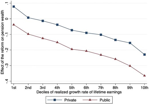
Distributional effects of the reform on pension wealth. The figure reports the effects of the reform on pension wealth against the deciles of realized growth rates of lifetime earnings, for a given cohort (born in 1960–1965), separately for public and private employees. The effects of the reform at the individual level are computed as the log difference of counterfactual pension benefits earned under the pro-rata and the earnings model, fixing retirement age at the pre-reform value.
While we rely on the reforms-induced variation in pension rules for private and public employees to estimate the model, in Online Appendix A.2, we also characterise the incentives brought about these reforms for the generality of self-employed.
5.2. Displacement Effect
We can use simulated wealth and pension benefits generated by the model to investigate the offset between discretionary and social security wealth. For each individual i in the simulated sample, we construct the effect of the reform on private wealth (|$\Delta A_{i,t}$|) and social security wealth (|$\Delta PB_{i,t}$|) at age t as the the percentage change between the simulated actual behavior in the presence of the reform (|$A^A_{i,t}$| and |$PB^A_{i,t}$| for private wealth and pension benefits, respectively) and the simulated counterfactual behavior in the absence of the reform (|$A^C_{i,t}$| and |$PB^C_{i,t}$| for private wealth and pension benefits, respectively).22 To obtain an estimate of the model-implied offset between private and social security wealth, we estimate the following equation on simulated data:
where |$\widehat{\delta ^A_1}$| indicates the response of accumulated savings for retirement to a variation in expected pension benefits predicted by the structurally estimated economic model.
To isolate the effect of changes in pension benefits on savings, we first estimate equation (9) for each cohort shutting off the retirement choice in the model (setting retirement age at the pre-reform value). Second, to understand the role of retirement in the offset, we conduct the same analysis allowing households to flexibly choose when to retire. We focus on simulated discretionary wealth at the end of working life (|$t=60$|).
Figure 2(a) reports the model-predicted percentage change in discretionary wealth following a 1% reform-induced variation in pension wealth for different timings of the reform over the working life (i.e. for different cohorts), obtained fixing labor supply. The comparison between the model-predicted response with fixed and flexible retirement is reported in Figure 2(b) (for the entire group of middle-aged workers, a specific cohort, and simulating the reform from the age of 25). Results obtained using changes in euros for both public pension and discretionary wealth are reported in Online Appendix Figure A16. The model predicts a 10|$\%$| decrease in benefit generosity induces an average increase in discretionary wealth at retirement of around 5.1% and 6.2|$\%$| for older and middle-aged workers, respectively. Clearly, these value should not be interpreted as estimates for the offset because the pension wealth shock occurred during the working life (at ages 53, 48,…, for the cohort of workers born in the years 1940–1944, 1945–1949,…, respectively). As expected, the response of private wealth to changes in pension benefit generosity decreases with the age at which workers face the pension wealth shock. Figure 2(a) shows then the extent to which older households are less willing to replace lost social security wealth with discretionary wealth, compared to what they would do were they facing the post-reform pension rules from the beginning of their working life. Online Appendix Figure A17 reports the percentage change in discretionary wealth before retirement (at age 60, “long run”) and 5 years after the introduction of the reform (“short run”), for each decile of reforms-induced variation in pension benefits.23 While the short-run response obviously understates the total effect on the accumulation of savings for retirement, the figure shows how bias increases with the (negative) variation in pension benefits.
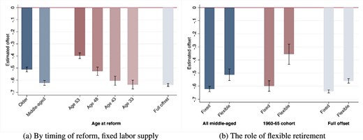
Response of discretionary wealth to changes in pension wealth. The figure reports OLS estimates for equation (9) on simulated data. Each bar corresponds to the point estimate for the model-predicted offset between public pension and discretionary wealth, in various counterfactual experiments. A total of 95% confidence intervals are also reported. Panel (a) reports the results for the offset by the timing of the reform over the households’ life-cycle, keeping retirement age at the pre-reform levels. The first two bars on the left correspond to the estimated offset for older and middle-aged workers, respectively. Bars 3–6 indicate the estimated offset for the cohorts of workers born in the years 1940–1944, 1945–1949, 1950–1954, and 1960–1964, respectively. The last bar on the right of panel (a) corresponds to the offset estimated for households that face the introduction of the reform at the beginning of the working life. Panel (b) compares the offset shutting off endogenous retirement and allowing for flexible retirement choices of middle-aged workers (first two bars on the left), the cohort of workers born in 1960–1964 (bars 3 and 4) and households that face the introduction of the reform at the beginning of the working life (bars 5 and 6).
To rule out the bias from observing households with varying planning horizons (Gale 1998) and obtain the model-predicted offset between public pension and discretionary wealth, we use the estimated model to simulate the introduction of the reform at age 25. The estimated model predicts an offset between discretionary wealth and social security wealth of around -0.64. This value falls in the ballpark of the estimates in the literature (see, e.g. Bottazzi, Jappelli, and Padula 2006 and Alessie, Angelini, and van Santen 2013), and suggests the displacement effect between public pension and private wealth is lower than one also in a model with perfectly informed and financially sophisticated individuals. Figure 2(b) shows that the model-predicted response of discretionary wealth to public pension wealth shocks is softened when households can flexibly choose when to retire. Specifically, the estimated model predicts an offset between public pension and discretionary wealth of around |$-0.55$| when labor supply is allowed to vary, significantly lower than that predicted in the case of fixed labor supply.
5.3. The Response of the Retirement Age
What is the role of the retirement age in explaining households’ savings responses to pension wealth shocks? In the post-reform regime, households can access higher pension benefits by retiring later. As shown in Section 4, the model-predicted response of households to the pension reforms in terms of savings for retirement and stock market participation is consistent with an increase in the retirement age (as well as the expected age of retirement of middle-aged workers elicited in the SHIW data).
To investigate the importance of retirement decisions against shocks to pension wealth, we exploit the simulated percentage change in pension benefits induced by the reform (at the age of 60, i.e. the retirement age in the pre-treatment period) across middle-aged workers, and the simulated effect on retirement age (constructed as the difference between the simulated post-treatment retirement age and the retirement age in the pre-reform regime.) We estimate the following simple equation using simulated data:
where |$\Delta \log \it{RET} = \log \it{RET}^A -\log \it{RET\,}^{C}$| is the log change in the age of retirement (in years), at the individual level, in the presence, and in the absence of the policy change. |$\widehat{\delta ^R_1}$| represents the simulated response of retirement to changes in the generosity of the social security system. We find a value of |$\widehat{\delta ^R_1} = -0.085$|. The model predicts then households to increase the retirement age by around 0.9% (about 0.5 years) following a 10% decrease in the pension benefits they would receive for a given age of retirement. This is one of the first quantification of the pension wealth effect on retirement exploiting variation in benefit generosity.24
Figure 3 plots the increase in retirement age in years by deciles of variation in pension benefits induced by the pension reform, showing the extent of the labor supply responses to a reduction in expected pension benefits (for a given retirement age) predicted by the estimated model. The model predicts individuals to work up to 3 years longer to offset the reduction in benefit generosity.
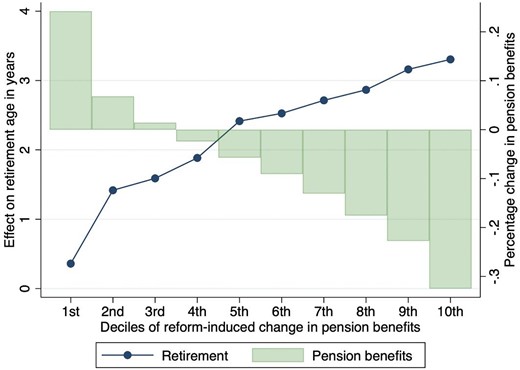
The extent of insurance through the retirement age. Each point corresponds to the model-predicted response of retirement to changes in pension wealth, in each decile of reform-induced variation in pension benefits. The response is expressed as the difference between the simulated retirement age under the post-reform NDC scheme and that under the pre-reform defined benefit regime.
5.4. Life-Cycle Welfare Effects
As discussed in Section 5.1, the effects of the reforms on pension wealth are substantially heterogeneous across the distribution of realized lifetime earnings growth. Further, the reform hit the different cohorts of households in different moments of their life cycle. The later in the working life households face a reduction in expected pension wealth for a given retirement age, the smaller their ability might be to close the gap between the optimal amount of discretionary wealth they accumulated in the pre-reform regime and that they would have accumulated had they faced the post-refom regime since the beginning of their working lives.
To study the potential distributional welfare effects of the reforms, we use a welfare metric similar to Low, Meghir, and Pistaferri (2010).
We compute the counterfactual lifetime utility from |$t_{1995}$|, the (cohort-specific) age at which the pension legislation occurs, to T in two settings, had the change actually occurred (|$m=A$|) or not (|$m=C$|), using the corresponding simulated decision profiles:
Following Low, Meghir, and Pistaferri (2010), we define |$\zeta _i$| as the fraction of consumption needed to make an individual indifferent between the |$m=A$| and |$m=C$| settings:
from which we can derive |$\zeta _i = 1-(E_{t_{1995}} U_i^{C}/E_{t_{1995}} U_i^{A})^{1/(1-\gamma )}$|. We interpret |$\zeta _i$| as the consumption-equivalent welfare effect of the reform.
The average value of |$\zeta$|, for each cohort-sector of employment group, is reported in Online Appendix Table A9. Because of the exogenous average reduction in lifetime resources, the introduction of the pension reform induced a welfare loss on average. Also, because of the greater reduction in pension benefits for a given retirement age faced by public employees (mainly due to the more generous pre-treatment pension provisions), workers employed in this sector experienced larger welfare losses.
Most importantly, the welfare analysis shows that households experienced a larger welfare loss the closer to the (pre-treatment) retirement age they are when the policy change is introduced, conditional on treatment status. Clearly, since different cohorts of households faced heterogeneous variations in expected pension wealth due to the reform, these heterogeneous welfare losses across cohorts may be just the consequence of the specific pension policy design.25 Figure 4 reports the welfare effects by deciles of reforms-induced variation in pension benefits, separately for the 1940–1944, 1950–1954 (i.e. older workers), 1955–1959, and 1965–1969 (i.e. middle-aged workers) cohorts (facing the introduction of the reform at different ages).26 First, the graphs show the large within-cohort heterogeneity in the welfare effects of the reforms across the distribution of reforms-induced variation in pension benefits. Second, they provide a representation of the life-cycle welfare effects of the pension reforms, with households that face the introduction of the reform at older ages experiencing larger welfare losses, conditional on the same (and for any level of) reduction in pension benefits generosity. These life-cycle effects are substantial. Households experiencing an above-median reduction in pension benefits would be willing to pay, on average, around 3% of annual consumption to face the same pension wealth shock 10 years earlier in their working life.27
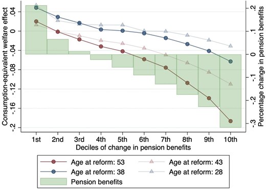
Welfare effects by changes in pension benefits and age at the time of reform. Each point corresponds to the model-predicted consumption-equivalent welfare effect of the reform |$\zeta$|, in each decile of reform-induced variation in pension benefits. The consumption-equivalent welfare effects of the reform are reported separately for households belonging to different year-of-birth cohorts, facing either a post-reform defined benefit pension scheme (reform at ages 53 and 43) or a post-reform pro-rata NDC regime (reform at ages 38 and 28).
In the model, this effect quantitatively depends on the degree of decreasing marginal utility of consumption and the utility cost of work. When exposed to the same reduction in expected social security wealth, older households need indeed to increase the saving rate more than younger households to achieve the same level of accumulated private wealth at (a given age of) retirement.28 However, in the presence of uncertainty and risk aversion, households find it costly to adjust their consumption response as much as it would be necessary to accumulate the amount of savings for retirement that they would have accumulated had they faced the same policy rules from the beginning of their working lives. The model quantifies the extent to which older households find it optimal to decrease current consumption more than younger households (and then the greater welfare losses) following the same decrease in expected pension benefits.
5.5. Early Retirement Age and Benefit Generosity
To shed further light onto the social security wealth effect on retirement and the displacement effect between private and social security wealth, we use the estimated model to study the responses of households to two pension policies that a legislator may consider to increase the financial sustainability of the social security system during the demographic transition: (i) an increase in the early retirement age; (ii) a reduction in benefit generosity. We simulate the introduction of the policy reforms starting from the defined contribution regime in place in Italy in 2013, in which workers can choose to retire between 57 and 70 years of age with pension provisions increasing with age (for a given amount of contributions), separately for cohorts of workers aged 40 and 55 at the time of reform.29 Specifically, the first policy change consists in an increase of the early retirement age to 62, while the second reform reduces the coefficients transforming total pension wealth contributions into annuities by 10%.
Panel (a) of Figure 5 plots the simulated labor supply effects of the increase in the early retirement age from 57 to 62, while panel (b) plots the predicted labor supply responses to the |$10\%$| decrease in benefit generosity. Similarly, Figure 6 compares the effects on the accumulation of discretionary wealth from the two reforms (panel (a) for the increase in early retirement age and panel (b) for the the decrease in benefit generosity).
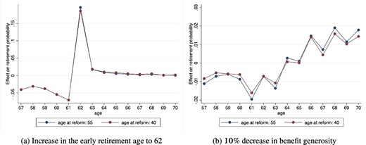
Effects on the probability to retire at a given age of alternative reforms. The graphs plot the model-predicted retirement response, expressed as the percentage point change in the probability to retire at a given age, when switching from the baseline NDC scheme to the post-intervention regime (panel a: The baseline regime when the minimum early retirement age is increased to 62; panel b: The baseline regime when benefit generosity is decreased by 10%).
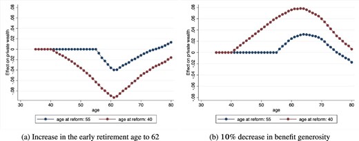
Effects on private wealth accumulation of alternative reforms by age. The graphs plot the model-predicted effects on private wealth, expressed as the percentage change in simulated private wealth, by age of the household head, when switching from the baseline NDC scheme to the post-intervention regime (panel a: The baseline regime when the minimum early retirement age is increased to 62; panel b: The baseline regime when benefit generosity is decreased by 10%).
The results show the substantially different implications of the two alternative policy changes. First, while increasing the early retirement age only induces a (mechanical) increase in the retirement age for those workers that would have retired before 62 in the pre-reform regime (without much differences between different cohorts of workers), decreasing the benefit generosity increases the retirement age, for any given level of pre-reform retirement age up to 70 years of age. Further, the model provides a quantitative assessment of the “life-cycle” wealth effects on labor supply, with younger cohorts of workers delaying retirement less than older workers to accumulate higher pension wealth. As shown in panel (b) of Figure 6, this is due to the fact that younger households optimally accumulate more wealth than older workers at retirement in response to the same decrease in benefit generosity.
Figure 6 also highlights the stark divergence in the response of households in terms of discretionary savings for retirement to the different pension policy changes. On one hand, decreasing benefit generosity induces households to increase savings for retirement. On the other hand, because households that would have retired before 62 years of age are now constrained to retire later (and then access higher pension provisions once retired), they optimally choose to reduce the savings rate. The model shows then substantial wealth effects on consumption from increasing the minimum age for early retirement in the presence of benefit generosity increasing with retirement age.
5.5.1. Heterogenous Effects across the Wealth Distribution
Panels (a) and (b) of Figure 7 show the effects on retirement of increasing the minimum age for early retirement and decreasing benefit generosity, respectively, by wealth quintiles at the time of reform.
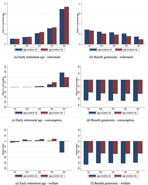
Early retirement age and benefit generosity—effects across the wealth distribution. The graphs plot the model-predicted effects on retirement (top panels), consumption (middle panels), and welfare (bottom panels). The left (right) panels depict the effects of increasing the minimum early retirement age to 62 (decreasing pension benefit generosity by 10%). The simulated effects are reported separately for cohorts of workers facing the policy change at 40 and 55 years of age. Each bar corresponds to the simulated effect in each wealth quintile at the time of the reform.
The model predicts substantial heterogeneity in the labor supply response at retirement to the increase in the early retirement age across the wealth distribution, with households in the top wealth quintile responding more (and with the heterogeneity in the response being larger when households face the policy change later in the working life). In contrast, decreasing the benefit generosity increases retirement age less the higher the ranking of households in the wealth distribution.
In the model, this result reflects the circumstance that, prior to the policy change, households in the upper part of the wealth distribution were choosing to retire earlier due to the fixed costs of working, and the marginal utility gains from working decreasing with wealth.
The model also shows that the legislator’s choice about the policy instrument to govern the demographic transition can have sizable consequences in terms of consumption and welfare inequality.30 First, while increasing the early retirement age induces an increase in consumption in the upper part of the wealth distribution (panel c, Figure 7), the decrease in benefit generosity induces a rather homogeneous consumption response (panel d). Further, the model shows that the increase in consumption inequality from increasing the early retirement age (i.e. an increase in consumption among those consuming more—see Online Appendix Figure A20 for baseline consumption across the wealth distribution) is larger the later households face the introduction of the policy change.
Finally, the model predicts the two alternative pension policies to have different welfare implications. While a decrease in benefit generosity induces substantial welfare losses across the entire wealth distribution (slightly increasing the lower the level of wealth at the time of reform), as shown in panel (f) of Figure 7, increasing the minimum age for early retirement affects mainly the welfare of households at the top of the wealth distribution at the time of reform, as shown in panel (e) of Figure 7. Further, the estimated model shows the two options for pension reform have different implications in terms of life-cycle welfare effects, with the latter mostly emerging following a variation in benefit generosity.
6. Discussion and Conclusion
This paper proposes an evaluation approach to pension policies that combines ex-post and ex-ante evaluation methods. We estimate a dynamic life-cycle model of savings, portfolio choice, and retirement using the reduced form effects of a wave of major pension reforms carried out in Italy in the nineties. The estimated model mimics pre-reform statistics and the effects on asset accumulation and participation rates in the financial markets estimated exploiting a DiD identification strategy, complementing previous evidence about the displacement effect between private and social security wealth. We also show that the estimated model predicts substantial social security wealth effects on retirement. Further, our framework suggests important life-cycle effects of the pension reforms, with older workers experiencing larger welfare losses, for any level of variation in benefit generosity. We use the estimated model to illustrate the substantially different consequences of alternative pension policies in terms of consumption and retirement wealth effects, as well as “life-cycle” welfare effects.
These results should be interpreted through the lenses of our assumptions on individual behavior. First, our model neglects the role of health. Clearly, there are several reasons why individuals’ health may affect their retirement behavior. However, although a large literature (starting from French 2005) has studied the impact of health on retirement, the existing evidence shows that health explains only a small fraction of the variation in retirement (Blundell, French, and Tetlow 2016b). Importantly, because our focus is on the interplay between households decisions and the financial incentives brought about the social security system, neglecting the role of health is problematic for our findings to the extent that changes in the pension rules have an effect on health. Some recent research have shown that increasing the minimum retirement age has positive consequences on individuals’ health (Bertoni, Brunello, and Mazzarella 2018). This suggests that the effects we find when simulating an increase of the minimum age for early retirement may represent a lower bound for the effect on the retirement age. While we believe that our findings represent first important evidence on the consequences of pension reforms for asset accumulation and retirement from a validated structural model, a promising avenue for future research is to extended this structural framework for pension policy analysis to incorporate the role of health. Second, our model assumes that all households are aware of the pension reforms and can optimally adjust their choices in response to the changing pension policy framework. As suggested by previous studies (e.g. Bottazzi, Jappelli, and Padula 2006), part of the population may have expectation error in terms of future replacement rates. Moreover, there is large evidence that financial knowledge is generally low in the population (see, e.g. Lusardi and Mitchell 2014). Limited financial knowledge and awareness about the policy changes may lead to understating the true behavioral responses using reduced form approaches.31 Hence, because we neglect the role of limited financial literacy, our structural estimation may be providing a lower bound for the cost of working with the consequence that the estimated model overstates (some) individuals’ labor supply response at retirement to the pension reforms. Financial literacy is more likely though to play a role in the distributional effects of the pension reforms, with heterogeneous responses to the pension reforms across the financial literacy (and wealth) distribution. Future research should explore the implications of allowing for endogenous knowledge accumulation on the response of households to pension policy shocks.
Our findings inform models of asset accumulation and social security about the importance of the retirement decision in response to shocks to pension wealth, and are relevant to studies considering the role of financial incentives for retirement. Further, we highlight and quantify the different trade-offs that policy makers need to consider when designing future pension policies, with important implications in terms of their acceptability among the population.
Acknowledgments
We thank the Editor and five anonymous referees for their comments. We also thank Irina Gemmo, Fedor Ishakov, Camille Landais, and Cormac O’Dea for helpful comments and suggestions. All the errors are ours. The project has been carried out while Mario Padula was charing the Commissione di vigilanza sui fondi pensione (COVIP), but the opinions expressed here belong solely to the authors. This paper was developed within the project funded by Next Generation EU—“Age-It—Ageing well in an agening society” project (PE0000015), National Recovery and Resilience Plan (NRRP)—PE8—Mission 4, C2, Intervention 1.3. Mario Padula is affiliated at CSEF.
Notes
The editor in charge of this paper was Nicola Pavoni.
Footnotes
Private pension funds were introduced in Italy in 1993, but social security—the first pillar—with its 33% contribution rate still plays the lion’s share in the Italian pension system. Pension wealth coincides with social security wealth for most households, due to the still limited degree of coverage of private pensions (approximately |$1/3$| of the working age population).
Blundell et al. (2016a) estimate the model comparing behavior of different cohorts facing different tax-credits and in-work benefits regimes. Low et al. (2018) validate the model against the empirical effects of a welfare reform after estimating the model using moments observed in the pre-reform period.
Online Appendix Figure B1 illustrates the NDC induces (in the most simplified setting) a decrease in the NPV of pension wealth at the pre-reform normal retirement age relative to the pre-reform DB system, and an increasing profile of pension wealth NPV over retirement age. We provide an extensive discussion of the reform’s impact on pension wealth in Section 5.1.
As discussed in Section 2.2, the reform design implies middle-aged workers are observed, at any given age, later on average than older workers (see Online Appendix Figure A1). Therefore, the vertical distance between the dashed and the continuous lines in Online Appendix Figure A13 does not allow to separate cohort from time effects. Although it is in general not possible to disentangle year, age, and cohort effects without additional information, the overlaps can still provide some insights about differences in life-cycle profiles of the two cohorts.
We define as pre-treatment period the years before 1992 (|$POST=0$|), when the first intervention was made, and as post-treatment period the years after 1995, |$POST=1$|. We drop transitional years 1993–1995.
We apply the baseline sample selection described in Online Appendix C.
We impose zero correlation between shocks to risky returns and labor income. While complicating the analysis a non-zero correlation makes little difference in the portfolio rule and thus on the households’ simulated portfolio allocations; see Gomes and Michaelides (2005).
In the pre-reform regime, |$H_N$| corresponds to the last year of earnings for individuals employed in the public sector (|$h_1=0$| and |$h_2=1$|) and to the average of the last 5 years of earnings for individuals employed in the private sector (|$h_1=0.8$| and |$h_2=0.2$|). Therefore, equation (4) approximates the private sector, pre-reform rule.
These contribution rules reproduce those in the actual institutional setting. The Italian system identifies a list of contingencies, including unemployment, job mobility, and disability, during which the State contributes on the individual defined contribution account in lieu of workers and employers. For this reason, we assume a working household to contribute to the defined contribution account in each period (up to age 56) in the post-reform regime.
Online Appendix Figure B1 illustrates the earnings model provides strong incentives to retire as soon as the worker meets eligibility criteria: retiring after the normal retirement age decreases the NPV of pension wealth.
Similarly to O’Dea (2018), |$\Xi$| wealth is a state variable only up to age 56 (when the retirement decision becomes available), with defined contribution benefits |$\Gamma$| being a state variable only after age 56. The transition from defined contribution wealth to defined contribution benefits at age 56 is governed by the equation:
Online Appendix Table A8 reports average simulated replacement rates for selected sub-groups of households.
A similar approach is adopted to estimate the age profile of stock market participation, employing a linear probability model.
Since the domain of the parameters |$\phi _1$| and |$\theta$| corresponding to a given level of utility cost of work and marginal propensity to bequeath, respectively, depends on the values of |$\beta$| and |$\gamma$|, to increase the efficiency of the estimation algorithm, we estimate the utility cost of work |$\tilde{\phi }_1$| and the marginal propensity to bequeath |$\tilde{\theta }$| instead. For a given set of parameter values, we back out |$\phi _1$| and |$\theta$| using |$\phi _1=(1-\gamma ) \log (1-\tilde{\phi }_1)$| and |$\theta = (1/\beta (1+r_f))[(1/\tilde{\theta }-1 ) (1/(1+r_f)) ]^{-\gamma }$|.
The approach addresses the small sample bias issues from the adoption of the optimal weighting matrix shown by Altonji and Segal (1996).
Higher values have been employed in the calibration of life-cycle models when trying to match financial market participation rates over the life-cycle, as in Fagereng, Gottlieb, and Guiso (2017).
We obtain this range converting the median estimates of $350 (in 1983 dollars) for 1994 and $500 for 1989 in 2010 euro.
The estimate for the utility cost of working corresponds to a value of |$\phi _1$| of around 0.09.
Details on the computation of the confidence intervals are reported in Online Appendix F. We follow Low and Pistaferri (2015) with this approach to evaluate the goodness of fit.
Middle-aged workers will become eligible to claim benefits for early retirement starting from around 2030.
Notice that percentage changes in pension benefits equal percentage changes in social security wealth, provided that pension benefits are constant after retirement and assuming that the pension reform does not affect the individual survival probabilities. In Online Appendix A, we also report results on the offset obtained using euro changes in discretionary and public pension wealth.
The ranking considers the percentage change in pension benefits induced by the reform.
Few studies have documented the impact of real-world reductions in benefit generosity on (the extensive margin of) labor supply. Krueger and Pischke (1992), Snyder and Evans (2006), and Gelber et al. (2017) empirically study the effect of benefit generosity on employment exploiting the lower benefits of the cohort of US individuals born in the period 1917–1922. While the former study finds no evidence of benefit generosity on employment, the last two find considerable labor supply responses that might understate the true effects from increasing benefit generosity because of limited awareness about the policy change among the affected cohorts. Further, Manoli and Weber (2016) provide non-parametric evidence of substantial retirement decisions response to financial incentives using data from Austria.
Under the pro-rata model, the later in the working life the middle-aged worker was in 1995 the larger the share of pension wealth computed with the earnings model.
As above, to capture the change in benefit generosity and isolate it from the effect of endogenous labor supply responses, the variation in pension benefits is computed given the pre-reform retirement age (60). Deciles of variation in pension benefits are defined using the distribution for the whole population, such that the magnitude of pension wealth change is constant within decile across groups.
This is computed as the average of the differences in consumption-equivalent welfare effects between the 1940–1944 and 1950–1954 cohorts of older workers (facing the reform at ages 53 and 43) and between the 1955–1959 and 1965–1969 cohorts of middle-aged workers (facing the reform at ages 38 and 28).
Online Appendix Figure A18 shows the extent of heterogeneity in the average consumption response to the pension reform (from the time of the introduction of policy change to retirement) between households belonging to the different cohorts.
We conduct these policy experiments for private employees, as the differentiation is mostly relevant due to the pre-reform heterogeneity in pension rules (as shown in Section 5.1).
We take the median log variation in annual consumption (measured as the difference between consumption under the alternative option for pension reform and the counterfactual consumption in the baseline) in the years following the policy change. The welfare effects are computed as detailed in Section 5.4.
On the role of frictions in the attenuation of estimated responses see; for example, Chetty (2012).
