


Abstract
This paper investigates the consequences of bureaucratic discretion in public procurement. I exploit a Hungarian policy reform, which allows a “high-discretion” procedure below a certain contract value. At the threshold, I document large discontinuities both in procurement outcomes and in the density of contract values, which indicates that buyers manipulate contract values to avoid auctions. I combine the reform and a structural model to find that discretion increases prices and results in the selection of less productive contractors. I also show that high discretion benefits firms with connections to the party of the central government. I use the structural model to document that public buyers are willing to sacrifice more contract value to increase their discretion if more connected firms are operating in the market. I also use the model to simulate the effects of counterfactual procurement thresholds on different procurement outcomes.
A set of Teaching Slides to accompany this article is available online as Supplementary Data.
1. Introduction
Public procurement accounts for 12% of the GDP in OECD countries (OECD 2016). Despite its importance, our understanding of the optimal design of public procurement is still limited. The ideal level of bureaucratic discretion is an especially controversial aspect of the optimal procurement design. On the one hand, if the interests of procuring officials and the public are not perfectly aligned, bureaucratic discretion increases the risk of corruption and the misallocation of contracts to politically connected winners. In light of this, it is not surprising that most developed countries use formalized procedures, such as open auctions, to constrain bureaucratic discretion (Chong, Staropoli, and Yvrande-Billon 2011; Tran 2011). On the other hand, auctions usually take more time and are more costly to organize than less formalized procedures, such as direct negotiations. Moreover, recent research on relational contracts in procurement has shown that information asymmetries and noncontractible quality dimensions may make a certain level of discretion necessary to create incentives for good contract execution (Kelman 1990; Bajari and Tadelis 2001; Calzolari and Spagnolo 2009; Kang and Miller 2015).
This theoretical ambiguity makes the net effect of discretion on procurement outcomes a critical empirical question. However, due to identification challenges, the existing empirical evidence is also inconclusive. Indeed, the lack of exogenous variation in bureaucratic discretion constitutes an important problem for any attempt to establish causality. Since the procurement procedure is not randomly determined but rather typically chosen by the procuring agency, the competence and integrity of the agency as well as the nature of the project may affect the level of discretion, thus creating a selection bias.
This paper fills this gap by proposing a novel solution to the identification problem. A standard approach to deal with the endogeneity of the procurement procedure is to exploit a “simplified acquisition threshold” in the value of the transaction. However, this solution is plagued by the manipulation of contract values and the sorting of tenders around the threshold. To deal with this problem, I develop a portable method that uses the time variation of a policy reform to structurally estimate a Roy model of the procurement procedure choice, which allows me to disentangle the causal effect of discretion from the sorting of tenders into high-discretion procedures. Building on this method, I document that discretion has a pivotal effect on contractor selection and I provide suggestive evidence identifying politicians’ self-interest as a likely underlying mechanism. The potential applications of this empirical strategy go beyond public procurement and it can provide a widely applicable remedy for the problem of manipulated running variables in cases where time variation in the size of the threshold is available.
I analyze the impacts of discretion in the context of a Hungarian policy reform enacted in 2011, which relaxed the obligation of using an open auction if the anticipated value of the transaction is less than 25 million Hungarian forints (approximately 90,000 USD). Below the 25 million threshold, buyers can choose an invitational procedure, which provides strong discretionary power in selecting potential bidders.
I start my analysis by presenting two important reduced form findings to illustrate public agencies’ reactions to the policy reform. First, I compare the pre- and post-reform distributions of anticipated contract values. In the post-reform period, I document a large spike below the threshold that was absent before the reform. This excess mass of procurement tenders below the threshold seems to originate from above the threshold where there is a missing mass relative to the pre-reform period. This change in the distribution suggests that some public agencies set contract values strategically to avoid open auctions.1 Second, following Coviello, Guglielmo, and Spagnolo (2017), I use a regression discontinuity design (RDD) to document that procurement outcomes are different on the two sides of the value threshold. I find discontinuities in all outcomes; tenders below the threshold have generally less favorable outcomes than those above. For instance, prices—measured by the log-ratio of the winning bid and the anticipated value—are larger and competition is weaker below than above the threshold. Moreover, below the threshold, buyers choose less productive contractors, who are more likely to be connected to the right-wing administration.
Although the regression discontinuity (RD) estimates reveal differences in procurement outcomes between the two sides of the threshold, these results cannot be interpreted as causal evidence. The ideal experiment for estimating the causal effects would require a random assignment of procurement procedures to tenders. The RDD, however, fails to deliver this because—as I show—contracts are systematically sorted across the threshold and therefore are not comparable. For example, there are good reasons to assume that corrupt agencies have a larger demand for discretion, so we may find more of them below than above the threshold. Similarly, procurers of more complex tenders may feel the obligation of using open auctions more burdensome, thus creating a difference in complexity between the two sides of the threshold. Sorting may also be driven by agencies’ heterogeneous administrative capacities.2 Consequently, discontinuities in the outcomes reflect the combination of discretion’s effect and the sorting of tenders around the threshold.
To address potential sorting around the threshold, I exploit time variation in the procedural requirements created by the policy reform. Since the reform introduced the high-discretion procedure only below the threshold, one might be tempted to use a simple difference-in-differences design. In this approach, tenders below the threshold, where the new policy made the high-discretion procedure available, belong to the treatment group, while tenders above the threshold, still obligated to use auctions, belong to the control group. However, the control group is also affected by the policy change through the outgoing selection of tenders. To address this problem, I develop a new method combining the difference-in-differences design with a Roy (1951) model of public agencies’ procurement and contract value decisions. The model is built on two key assumptions: (i) the cost of manipulating the contract value is increasing in the size of the manipulation, and (ii) the benefit from discretion—therefore from manipulation—is a continuous and monotonic function of outcome-relevant unobservables.
I estimate the model in two steps. In the first step, I nonparametrically estimate the extent of sorting into the high-discretion procedure by incorporating information on the change of the contract value distribution over time. In the second step, I construct a control function from the first step estimates—following Heckman (1979)—to disentangle the causal effect of discretion from the effect of sorting. The logic of the identification is somewhat similar to that found in Diamond and Persson (2016), which estimates the effect of teacher grade manipulation on student outcomes by comparing both the outcomes and the grade distribution to manipulation-free counterfactuals. However, unlike Diamond and Persson, I use the pre-reform period to generate the counterfactual distribution. The intuition behind the identification is the following. If we compare open auctions across time periods, we find a large compositional change of tenders below the threshold, where discretion becomes easily available, thus causing many tenders to sort into the high-discretion procedure. Conversely, as we move further above the threshold, discretion requires a large distortion of the reported contract value, making sorting less popular. The comparison of open auctions across time at different points of the contract value distribution, exposed to a varying degree of compositional change, identifies the effects of sorting.
Causal effects detected by the structural model are qualitatively similar but quantitatively different from correlations captured by the RDD. My estimates show that discretion increases the price of contracts by 6 percentage points, decreases the number of bidders by almost 1, and results in the selection of 28% less productive contractors. However, this effect is only a third of the RDD result, which implies that the sorting of low-productivity tenders—into the high-discretion procedure—accounts for two thirds of the discontinuity at the value threshold. I also find that discretion increases the probability of a right-connected winner by 11 percentage points.
These findings show that agencies use discretion to favor less productive but politically more connected firms. However, this is not a direct evidence for the corrupt use of discretion since connected and unconnected companies may differ in many unobserved dimensions. There could be numerous benefits of awarding contracts to connected firms. I test for several potential benefits, and find no evidence for them. First, I use proxies of ex-post contract execution, such as post-award contract modifications, delays, and ex-post prices, to study potential trade-offs between ex-ante (e.g. price, contractor productivity) and ex-post procurement outcomes. Although there may be a trade-off between price and unobserved quality, I find no correlation between prices and observable measures of contract execution. However, I find that less productive contractors, if anything, are associated with worse ex-post contract execution. Second, I show that domestic and local firms do not benefit from discretion; thus, agencies do not use discretion to stimulate the local economy. Third, discretion has a negative effect on the winning chances of incumbent contractors suggesting a limited role of relational contracts. Fourth, results on firm age and exit imply that discretion reallocates contracts to companies with shorter lifespans. This finding is inconsistent with an increase in unobserved firm quality but in line with journalistic accounts of high turnover among politically favored companies.
Since the high-discretion procedure is not available above the threshold, the excess mass below the threshold carries information on the trade-off between choosing the discretionary procedure and obtaining the optimal contract value. Although the non-parametric strategy mentioned above identifies the demand for discretion without any functional form assumptions, it fails to identify this trade-off explicitly. To address this shortcoming, I propose a fully parametric approach to identify deep parameters of the procuring agency’s utility.3 This approach expands the analysis in two important directions: (i) it allows to include tender level controls to investigate associations between tender characteristics and the demand for discretion and (ii) it helps to explore the consequences of alternative procurement policies. Following the parametric approach, I find that demand for discretion is positively associated with the share of connected companies operating in the market. More specifically, in markets with a 1 percentage point larger share of connected companies, agencies—with unmanipulated project sizes above the threshold—are willing to sacrifice 0.6%–0.9% more contract value to obtain discretion. This finding is in line with the political favoritism interpretation of the main results. I also find that the sorting of low-productivity tenders into high discretion is partly—though not entirely—explained by observable tender level characteristics such as agency type or the sector of the good purchased.
I also use the parametric model to conduct policy simulations. First, I simulate the effects of counterfactual procurement thresholds on price and contractor productivity. Second, I investigate how regulatory oversight interacts with the threshold value. The first set of simulations highlight the important new insight that the size of the threshold affects outcomes through two different channels. First, it affects outcomes directly by making the high-discretion procedure more widely available. Second, by changing the distribution of contract values, it changes the relative weights of tenders with different characteristics, thus affecting the value weighted average outcomes. On the basis of my simulations, prices increase monotonically in the size of the threshold but productivity is maximized by a small but positive (7 million forints) threshold. The simulation suggests that the procurement reform of 2011 increased average prices by 2.3% and decreased average productivity by 3.5%. Simulations on regulatory oversight suggest an interesting interaction between increasing the procurement threshold and improving government scrutiny to prevent agencies from distorting contract values.
This paper most directly contributes to the literature that investigates the effects of discretion in public procurement (Lalive and Schmutzler 2015; Chever, Saussier, and Yvrande-Billon 2017; Coviello, Guglielmo, and Spagnolo 2017; Carril, Gonzalez-Lira, and Walker 2020; Decarolis et al. 2020a; Baltrunaite et al. 2021; Coviello et al. 2022). Many studies of this literature have exploited similar value thresholds using either a RDD or a difference-in-differences design. The challenge with these strategies, as I discussed above, is that in the presence of sorting they fail to identify the causal effect of discretion. My contribution to this literature is twofold. First, I study direct measures of contractor characteristics, which allows this paper to complement our understanding with allocative efficiency considerations. Second, although much of the previous work exploit procurement thresholds, to my knowledge, this is the first study to systematically address the problem of manipulation at threshold by employing a structural model. This empirical strategy is transferable to other contexts in which the RD design is plagued by the manipulation of the running variable, but there is time variation in the size of the cutoff.4
The paper speaks to a recent experimental literature exploring the broader context of bureaucratic discretion. For instance, Bandiera et al. (2021) investigate the optimal allocation of authority in organizations and find that increasing the autonomy of lower level bureaucrats—at the expense of the authority of their monitors—increases efficiency. This paper complements their findings by exploring the consequences of different procedures at a fixed organizational structure.
My study also contributes to the line of research investigating the determinants of the demand for discretion. For example, Palguta and Pertold (2017) document the manipulation of contract values to avoid auctions in the Czech Republic and find a higher fraction of anonymously owned firms among the winners of manipulated contracts. Tóth and Hajdú (2017) document similar anomalies in contract values in Hungary and link them to an increased risk of corruption. Decarolis et al. (2020a) find that government officials investigated by the police for corruption choose discretionary procedures more often. Gerardino, Litschig, and Pomeranz (2017) find that rigorous audits increase procurers demand for high-discretion procedures. Zamboni and Litschig (2018) also highlight the importance of private interests by showing that restricted procedures are more likely to involve corruption compared to unrestricted procedures in Brazil. This paper contributes to this literature by providing evidence consistent with political favoritism.
I also build on the literature of political favoritism in procurement (Goldman, Rocholl, and So 2013; Muraközy and Telegdy 2016; Baltrunaite 2020; Brogaard, Denes, and Duchin 2021). My results speak to this line of research by showing that favoritism is sensitive to certain elements of the policy environment. I also contribute to studies quantifying the efficiency consequences of favoritism (Bandiera, Prat, and Valletti 2009; Mironov and Zhuravskaya 2016; Schoenherr 2019; Szeidl and Szucs 2021) by estimating the effect of procurement design on contractor productivity.
The rest of the paper is organized as follows. Section 2 describes the institutional context and my data. Section 3 presents the reduced form evidence. Section 4 describes the procurement model and the two different estimation strategies. In Section 5, I present my model estimates. Section 6 reports counterfactual simulations. Section 7 concludes the paper.
2. Context and Data
2.1. Public Procurement in Hungary
Hungary is one of the new member states of the EU. By Hungary’s 2004 accession to the EU, its national procurement legislation had been gradually harmonized with European directives. An explicit goal of the EU directives was to improve the transparency and competitiveness of the procurement process. In line with these efforts, the Procurement Act of 2003 named open auction as the most desirable procurement procedure, which could only be avoided under very specific circumstances. Indeed, during the 2003–2011 period more than two-thirds of public procurement contracts were awarded through open auctions. Similarly to other countries, these auctions used different assessment rules. About 40% of tenders used scoring auctions where the allocation of the contract is determined not just by prices but a combination of price and quality.
During my study period, Hungary had two consecutive administrations. Between 2002 and 2010 a Socialist–Liberal coalition was governing Hungary. After a series of scandals involving the prime minister, the Socialist government suffered a large decline in popularity. In 2010, the Conservative opposition won a landslide victory, capturing two-thirds of parliamentary seats. Relying on its unprecedented political power the new conservative administration enacted a long list of new laws, including the reform of the public procurement regulations.
Although open auctions are widely considered as the most transparent form of public procurement, they are typically slower and more costly to organize than simplified procedures providing more discretion. Since the temptation to engage in corruption increases with contract value, many countries, including the United States and most EU countries, use procurement thresholds allowing simplified procedures for small value contracts. Following these examples, in 2011 the Hungarian Parliament accepted a new Public Procurement Act enabling government agencies to choose an invitational procedure if the anticipated contract value was below 25 million Hungarian forints (about 90,000 USD).5 The anticipated value of a contract is set by the procuring agency before the procedure is selected by way of matching the approximate cost of the purchase. According to the standard procedure, agencies determine the value as the product of the desired amount and the price from the Procurement Authority’s price list. If the list price is not available, the agency has to document that the price used to compute the value is based on previous transactions or marketing research. The invitational procedure mentioned above provides the buyer more discretion to pre-select potential applicants,6 which clearly makes the procurement procedure simpler and faster7 but comes at the cost of less transparency and more opportunities for corruption.
2.2. Data and Descriptive Stats
The primary source of data is the cleaned public records of all Hungarian procurement contracts for the 2009–2015 period. This dataset contains the anticipated and actual values of procurement contracts and the name of the requestor agency and all bidders. Since the 25 million threshold does not apply to construction contracts, I only focus on non-construction tenders. From the total 48,654 contracts, I exclude 274 observations in which the number of bidders exceeds 30 since it suggests a framework agreement instead of an individual project.
Figure 1 plots the time trends of the number (panel a) and the aggregate value (panel b) of contracts awarded either by an invitational (which provides high discretion) or by other lower discretion procedures. In this latter category, 80% are open auctions, 7% are negotiations with an announcement, and the rest composed of a few other special procedures. As auctions and negotiations with an announcement provide no control over the pre-selection of applicants they are generally considered as low-discretion procedures. Figure 1(a) shows that the share of high-discretion tenders was negligible before 2012 and it increased substantially from 2012 onward. The figure also documents a fall in the number of low-discretion procedures in 2012 suggesting that agencies increasingly substituted auctions with high-discretion procedures. Figure 1(b) shows a similar pattern for the aggregate (anticipated) value. Between 2011 and 2013, the total value procured by high discretion increased by a factor of 10, while the value of low-discretion contracts decreased by more than 20%.
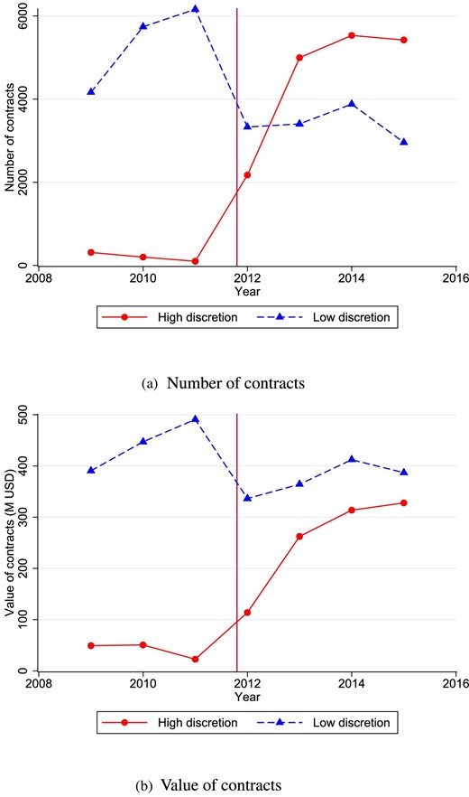
Number and aggregate value of high discretion and other tenders.
To evaluate the quality of contractors, I link awarded firms to their balance sheet data.8 I have balance sheet information on almost all Hungarian firms from the Hungarian Statistics Office for 2000–2012, and from the Hungarian Company Register for 2013–2015. These data also contain ownership shares for each firm by the following categories: central government, local governments, domestic private entities, and foreign entities. Moreover, the dataset also records the address of each firm’s headquarter, allowing me to compute the distance between the procuring agency and its contractor. I was able to match 86% of my sample of contracts to the balance sheet of the winning firm. Although the imperfect matching of contracts to balance sheets may raise concerns about sample selection bias, discretion is uncorrelated with the probability of a successful match, thus suggesting that potential sample selection is unrelated to the procedure.9
In my main specifications below, I focus on three main groups of variables. The first group aims to capture the strength of competition. I operationalize competition in two ways: first, I use the log-ratio of the actual reward and the anticipated contract value, which I refer to as the log-normalized price—similar to the winning rebate used by Coviello, Guglielmo, and Spagnolo (2017). This measure approximates the percentage gap between the winning bid and the anticipated contract value.10 Results on the log-normalized price may capture transfer effects by showing how much money is redistributed from taxpayers to firms by choosing a high-discretion procedure (potentially in exchange for better product quality or contract execution). However, interpretation of the results on the log-normalized price is complicated by potential manipulation of the anticipated value. I formalize these interpretation problems and report a specification robust to manipulation in Section 5.2. Second, as an alternative measure of competition, I also report results on the number of bidders.
The second group of outcomes is the productivity of the awarded firm. Since most firms sell their products in private markets too, productivity is a meaningful measure of firm quality as it may capture lower production costs or better product quality. I use several proxies of productivity: total factor productivity—calculated in multiple ways—and labor productivity measured by the ratio of added value and the number of employees. In the main specifications, I estimate parameters of the production function following Wooldridge (2009).11 As a robustness check, I also measure total factor productivity following Hsieh and Klenow (2009).
The presence of political favoritism may pose an additional threat to the correct measurement of productivity. Connected firms may win overpriced procurement contracts or get access to preferential loans (see Khwaja and Mian 2005) that would artificially inflate their productivity. This will create a spurious correlation between productivity and discretion if connected firms win high-discretion tenders more often. To address this issue, I compute the average TFP of winning firms for 2006–2009, the last 4 years before the conservative government came to power. Since the conservative party had less opportunities to favor connected firms before 2010, the lagged TFP of their crony companies is less inflated by the effect of political favors. Nevertheless, my estimates on productivity may be considered as lower bounds of the real effects of discretion.
Since my measures of productivity are revenue-based, they are driven by a combination of physical productivity and markups. To disentangle the two channels discretion may operate through, I measure markups following De Loecker and Warzynski (2012) to estimate the effect of discretion on markups and to include it as a control in certain specifications.
The third group of outcomes focuses on political favoritism. To document the impacts of political connections, in a joint project with Miklós Koren and Adam Szeidl, we develop a measure of connectedness for the 500 firms with the largest procurement revenue in the 2006–2014 period.12 The measure is created by a group of research assistants who manually checked the connections between companies and any of the parliamentary parties following two different strategies. First, they looked for matches in the full names of firm representatives and political candidates. The names of firm representatives are obtained from the Hungarian Company Register and they include three main groups: (1) Representatives who can sign legal documents in the name of the firms, typically top managers; (2) Owners; and (3) Board members. The names of political candidates are taken from the digitized public records of all national and local elections for the period from 1990 to 2014. In the case of matching names, we relied on the research assistants’ personal judgment to determine whether the name was rare enough to classify the firm as politically connected. Second, the assistants made manual Google searches on the names of each company to find any mention of personal connections between the firm and political parties in national or local news. Using this algorithm, I classify the top 500 procurement winners into three categories: connected to the right-wing administration, connected to the left-wing opposition, and unconnected. Online Appendix Table A1 reports observables of the average contractor and firms from the top 500 with different connections. Unsurprisingly, top 500 firms are very different from the average tender winner in every dimension. Unconnected (top 500) firms are somewhat larger, older, and slightly more productive than connected (either left of right) top 500 firms.
To further investigate the mechanisms, I also report results on a list of other outcomes. To assess discretion’s impact on the local economy, I look at the probability of domestic contractors and the physical distance between the buying agency and the winning company. I also report results on the size, age, and the exit rate of the awarded firms, which are widely used proxies of firm quality—since more successful firms grow larger and live longer (Syverson 2011). The literature on relational contracts highlights the advantages of using selection criteria based on past performance, which gives rise to stable procurer–contractor relationships and incentivize firms with the future value of these relationships (Levin 2003; Calzolari and Spagnolo 2009). In order to evaluate the importance of relational contracts, I show results on the probability of incumbent winners. I classify the winner of a tender as an incumbent if she has already received a contract from the same procurer in the three-year window before the given tender.
For a subset of contracts in the pre-reform period, I also have data—created by Fazekas, Tóth, and King (2016)—on ex-post measures of contract execution, such as post-award contract modifications, delays in delivery, and ex-post prices (normalized by the anticipated value). This database combines contract award notices with contract modification notices and contract completion announcements to provide information on the execution of procurement contracts. Unfortunately, not all announcements appear for the universe of contracts, therefore the contract execution measures are available to only a subset of contracts. Nevertheless, the data covers all product categories and allows me to investigate the associations between my baseline ex-ante—price and productivity of the awarded firm—and a list of ex-post procurement outcomes.
Table 1 presents means and standard deviations for all procurement outcomes by procedure type. Panel A of Table 1 displays tender-level characteristics. As expected from the nature of the value threshold, the average anticipated value of high-discretion tenders is smaller (by 3.6 million forints) than the average value of low-discretion tenders. Panel A also documents a fewer participants and a higher log-normalized price for high-discretion procedures. The winning bid is below the anticipated value by approximately 7% for high discretion and 13% for low-discretion tenders.
Tender and contractor characteristics for high- and low-discretion tenders.
| High discretion | Low discretion | |||
|---|---|---|---|---|
| Mean | Std. Dev. | Mean | Std. Dev. | |
| Panel A—Tender characteristics | ||||
| Anticipated contract value (M forints) | 15.8 | 12.2 | 29.5 | 29.6 |
| Number of bidders | 2.28 | 1.02 | 2.95 | 2.71 |
| Log(normalized price) | −0.071 | 0.224 | −0.130 | 0.293 |
| Panel B—Contractor characteristics | ||||
| Log(TFP) | 8.46 | 1.50 | 9.06 | 2.02 |
| Employment | 93 | 593 | 198 | 1008 |
| Firm Age | 13.5 | 8.5 | 15.1 | 8.8 |
| Domestic | 0.915 | 0.279 | 0.805 | 0.397 |
| Incumbent | 0.342 | 0.474 | 0.442 | 0.497 |
| Distance | 60.7 | 73.9 | 68.4 | 77.2 |
| Panel C—Political connection of contractor | ||||
| Right connected | 0.160 | 0.366 | 0.078 | 0.268 |
| Left connected | 0.028 | 0.165 | 0.025 | 0.156 |
| Unconnected | 0.429 | 0.495 | 0.476 | 0.499 |
| Panel D—Ex-post contract execution | ||||
| Ex-post contract modification | 0.178 | 0.383 | ||
| Delay in delivery (in days) | −4.48 | 210 | ||
| Ex-post log(normalized price) | −0.085 | 1.31 | ||
| Number of contracts | 18,742 | 29,638 | ||
Notes: This table reports means and standard errors of different tender and contractor characteristics for high and low-discretion tenders separately. Low-discretion tenders include open auction and negotiation with an announcement, while high discretion is an invitational procedure. Log(normalized price) is the log-ratio of the winning bid and the anticipated contract value, Domestic is an indicator for domestically owned contractors, Distance is the distance (in km) of the requesting agency and the contractor’s HQ, Incumbent is an indicator for contractors, which won contracts from the same agency–product category pair before. The share of right-, left-, and unconnected winners in Panel C is computed for tenders with at least one top 500 participant. Ex-post execution measures in Panel D are only available to a subset of contracts in the pre-reform period.
Panel B of Table 1 reports means and standard deviations of contractor characteristics. It shows that contractors awarded in high-discretion procedures tend to be smaller, younger, and less productive than contractors selected in low-discretion tenders. Moreover, winners of high-discretion procedures are more likely to be domestically owned but less likely to be incumbent winners than those selected in auctions. Panel C documents that high discretion is associated with more right-connected but slightly less unconnected winners. The shares of winners with different connection statuses are only presented for tenders with at least one top 500 participant.
Panel D, which only focuses on a subset of contracts in the pre-reform period, reports that 18% of contracts are modified ex-post, and they are executed on average 4.5 days before the deadline but there is substantial variation in delays. The ex-post prices of open auctions are larger than ex-ante prices suggesting that costs typically run over the ex-ante budget. On average, the ex-post value is about 8.5%—as opposed to the ex-ante 13%—below the anticipated contract value.
3. Reduced Form Evidence
In this section, I document some important patterns in the data. I show that the procurement reform, in addition to influencing agencies’ procedure decisions, affected the distribution of contract values and many procurement outcomes.
3.1. Distribution of Contract Values
Figure 2 plots the distribution of anticipated contract values. The dashed line shows the pre-reform, the solid line depicts the post-reform distribution. The left tails of the two distributions are very similar, but there is a large spike below the threshold in the post-reform period, which was absent before the reform. The excess mass of the spike seems to originate from above the threshold, where there is a missing mass relative to the pre-reform period. The main message of the figure is that some buyers set the contract value strategically below the threshold in order to avoid the open auction requirement. This claim is further supported by Online Appendix Figure A1(a), which plots the value distribution of low-discretion tenders for the pre- and post-reform periods. The absence of a spike below the threshold in Online Appendix Figure A1(a) confirms that the patterns of Figure 2 are driven by the high-discretion procedure.
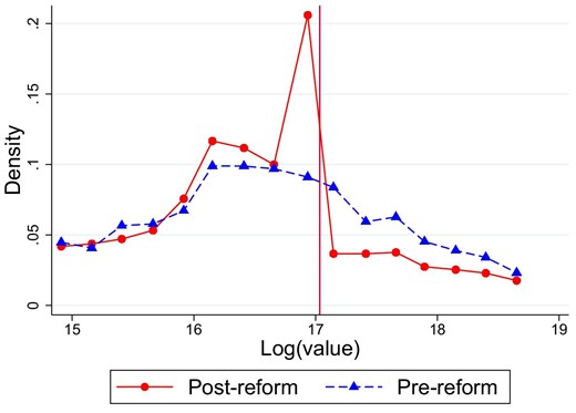
Distribution of log-contract values.
Procuring agencies can reduce reported value of a contract in two ways. Either they manipulate the list price used to calculate the reported value or they reduce the physical quantity of the goods purchased. The second strategy itself can be executed in two distinct ways. First, procurers can cut a contract into multiple pieces smaller than the threshold value. Second, they can make real changes in the size of the project to fit the contract value below the threshold. Although the Public Procurement Act strictly forbids the slicing of a project into several contracts, agencies can still try to increase the frequency of repeating purchases to reduce their size. To check the importance of slicing contracts, Online Appendix Figure A1(b) plots the distribution of project values aggregated to agency–contractor–period cells. By showing a very similar picture to Figure 2, Online Appendix Figure A1(b) suggests that cutting a project into multiple parts is not a common practice and agencies often use alternative strategies, such as manipulating the list prices or making real distortions to the size of their projects, to obtain more discretion over the selection of contractors.
The introduction of the threshold may also change the type of goods purchased if agencies replace larger projects with completely different smaller ones. Section A1.2 in the Online Appendix finds limited support for this claim by looking at the change of the composition of product categories over time.
Procuring bureaucrats may prefer to avoid open auctions for multiple reasons. On the one hand, the invitational procedure is faster and cheaper than an open auction, which requires more red tape and usually the review of more applications. Moreover, discretion may improve the noncontractible quality of the goods and services purchased and promote relation specific investments by securing stable procurer–contractor relationships. On the other hand, bureaucrats and politicians have private interests too and high discretion provides more opportunities for political favoritism. Results of the parametric estimation in Section 5.4 investigate this question by providing evidence on the associations between tender characteristics and the demand for discretion.
3.2. Procurement Outcomes
The procurement reform has introduced a discontinuity in the procedure requirements at 25 million forints. Before I turn to my main empirical strategy investigating the causal effects of discretion, I highlight the overall changes in procurement outcomes induced by the reform. First, I present evidence on the agencies’ compliance with the new rules. Figure 3 plots the share of high-discretion procedures as a function of the log anticipated value in the post-reform period. The large discontinuity in Figure 3 is a direct consequence of the new regulation, which relaxes the strict requirement of open auctions below (but not above) the 25-million threshold.
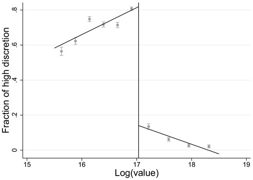
Fraction of high-discretion procedures in the post period.
Next, I document discontinuities in procurement outcomes at the threshold. Figure 4 plots a list of different procurement outcomes as a function of the log anticipated value in the post-reform period. The figure reports results on three main groups of outcomes: competition, productivity, and political favoritism. Figure 4(a) and (b) focus on competition by showing the log-normalized price and the number of bidders respectively. Figure 4(c) plots the total factor productivity of the selected contractor, while Figure 4(d)–(f) depicts the probability of a right-, left-, or unconnected winner. The top 500 firms (whose connection status we know) are much larger than the average contractor and tend to participate in open auctions more often, so the latter graphs focus only on tenders with at least one top 500 bidder. All figures show large differences in the outcomes at the threshold. In high-discretion tenders, buyers tend to pay more for the same anticipated value and they choose less productive contractors. Also, high discretion is associated with more right-connected and less unconnected winners, while the chances of left-connected firms seem to be unrelated to the procedure. These patterns suggest that buyer’s discretion may have a paramount effect on the selection of contractors.
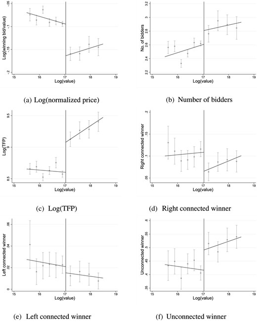
Discontinuities in procurement outcomes in the post-reform period.
To prove that discontinuities in Figure 4 are driven the policy reform, Online Appendix Figure A2 conducts a placebo test and reports the same outcomes for the pre-reform period. The figure shows that all procurement outcomes are continuous at the threshold, thus confirming that discontinuities of the post-reform period are indeed driven by the high-discretion procedure.
To quantify the size of the discontinuities and the implied correlations between discretion and procurement outcomes, Online Appendix A1.3 presents the results of the corresponding local linear regressions. The analysis shows economically large and statistically significant relationships between procurement outcomes and the high-discretion procedure.
Discussion.
Although we see large discontinuities at the value threshold, the question of whether there is a causal link between discretion and procurement outcomes remains open. In an ideal experiment, we would randomly choose the procurement procedure and measure the difference in the outcomes between tenders using different procedures. However, as a result of the manipulation in contract values around the threshold, assignment of tenders (and agencies) to below and above the threshold is not random. Indeed, the comparability of tenders on the two sides of the threshold breaks down if a specific group of public agencies has a higher demand for discretion thus sorts below the threshold. In this case, the discontinuities documented above do not reflect the true causal effects of discretion, but they are at least partially driven by the compositional differences between the two sides of the threshold.
4. Model of Procurement
4.1. Setup
My model, similar in spirit to Roy (1951), formalizes the idea that contracts can be systematically sorted into different procurement procedures. Public agencies choose procurement procedures with an eye on both their administrative costs and their effects on procurement outcomes. Agencies’ focus on outcomes may include benevolent motives, such as obtaining lower prices or better product quality, or illicit considerations, such as collecting bribes from the winning firms. Different agencies weight these considerations differently, thus giving rise to a selection based on the unobserved characteristics of agencies and contracts. In addition to procedures, agencies also control the anticipated value of contracts by choosing quantities and potentially manipulating list prices. Procurement thresholds make procedure and value decisions interconnected and create a trade-off between choosing discretion and the optimal contract value.
Formally, the procuring agency simultaneously determines the quantity of purchased goods and services q, the list price p, and the procurement procedure D. For each contract, |$\bar{p}$| denotes the exogenous unmanipulated list price. The procurement procedure is either a high-discretion procedure |$(D=1)$| or an open auction |$(D=0)$|.
The procuring agency’s utility from tender i is
where |$Y_i$| is a vector of observable procurement outcomes, and |$E(Y_i)$| is the value of these outcomes expected by the procuring agency prior to the execution of the procedure. |$\epsilon _i$| is a residual term capturing unobserved incentives to choose discretion, such as the administrative cost advantage of a high-discretion tender relative to an open auction. Observable factors relevant for the procedure choice (captured by |$Y_i$|) may include the price of the contract and the productivity or the political connections of the selected contractor. Obtaining a favorable price is clearly important but the contractor’s expected productivity is also a relevant factor since it may be correlated with product quality. Indeed, if a contractor also operates in the private market, higher productivity may signal either lower production costs or the company’s ability to sell its higher quality product at a higher price.13 The political connections of the awarded firm may matter by making the extraction of private rents cheaper for procuring officials.
The expression in equation (1) is also a function of quantity (|$q_i$|) since more supplies generally make it easier for public agencies to fulfill their mission. The utility also depends on the combination of real and manipulated list prices since any deviation of |$p_i$| from |$\bar{p}_i$| requires a costly manipulation and the bypassing of procurement guidelines.
The agency’s utility is both directly and indirectly affected by the procurement procedure. Directly because high discretion procedures typically have lower administrative costs (heterogeneity in this cost advantage is captured by |$\epsilon _i$|) and indirectly because expected procurement outcomes are also functions of the procedure chosen by the agency:
Equation (2) captures the idea that, by creating more competition and using more explicit selection criteria, auctions may result in different procurement outcomes than discretionary procedures. An open auction is generally expected to reduce prices and limit corruption but its impact on the productivity of the selected contractor is ambiguous. On the one hand, it can improve quality if the interests of procuring officials are misaligned from that of the public. On the other hand, in the presence of contracting difficulties, a more formalized procedure may be detrimental to contractor selection. I do not make any assumptions on the direction of this relationship and allow the data to dictate the sign of discretion’s effect on productivity. I assume, however, that the outcomes also depend on the unmanipulated contract value |$\bar{p}_iq_i$| since larger contracts may attract a different pool of applicants than their smaller counterparts. Finally, |$u_i$| denotes the outcome-relevant heterogeneity of tender i conditional on the contract value |$\bar{p}_iq_i$| and the procurement procedure |$D_i$|, which is observed by the procuring agency but unobserved by the econometrician.
By embedding the relationship given by equation (2) into equation (1), we can express the agency’s utility as a function of |$p_i$|, |$\bar{p}_i$|, |$q_i$|, |$D_i$|, |$\epsilon _i$|, and |$u_i$|:
Agencies maximize their utility under some constraints. Each project has an exogenous budget |$\nu _i$|. Variation in the budget captures heterogeneity in the nature of public projects. A small municipal government buying printing paper for the mayor’s office faces a small |$\nu _i$|, while the acquisition of a new fleet of police cars in a large city exemplifies a project with a large |$\nu _i$|. Procurers choose quantities subject to the budget constraint:
where the anticipated—unmanipulated—contract value on the left-hand side captures the agencies best guess of the contract’s cost.14
The public agency may operate under two alternative regimes. Under the first regime, which was in effect before the policy reform, high-discretion procedures are not available, meaning that |$D_i=0$| for all i. The second regime, similar to the regulation of the post-reform period, allows high-discretion procedures (|$D_i=1$|) as long as the reported value is below an exogenous threshold T, while keeps open auction compulsory above the threshold. Formally, it adds the following constraint:
where |$V_i \equiv p_i q_i$| is the reported value of the contract.
In order to keep the model tractable and identifiable, I make three assumptions about the utility function given by equation (3).
|$\widehat{U}(p_i, \bar{p}_i, q_i, D_i, \epsilon _i, u_i)$| is increasing in |$q_i$|.
Assumption 1 reiterates the idea already mentioned above that agencies benefit from buying more goods and services.
|$\widehat{U}(p_i, \bar{p}_i, q_i, D_i, \epsilon _i, u_i)$| is maximized if the actual list price—used for computing the anticipated value—is equal to the unmanipulated list price |$p_i =\bar{p}_i$|, and the utility is single peaked. Formally, |$\widehat{U}(\bar{p}_i,\bar{p}_i, q_i, D_i, \epsilon _i, u_i) \ge \widehat{U}(p_i, \bar{p}_i, q_i, D_i, \epsilon _i, u_i)$| for any |$p_i$|, and if |$p_1<p_2\le \bar{p}_i$| (or |$p_1>p_2\ge \bar{p}_i$|), then |$\widehat{U}(p_1, \bar{p}_i, q_i, D_i, \epsilon _i, u_i) < \widehat{U}(p_2, \bar{p}_i, q_i, D_i, \epsilon _i, u_i)$|.
This assumption captures the idea that the manipulation of the list price is possible but it is costly and its cost is increasing in the size of the manipulation. This assumption makes sense since list prices have to be based on previous transactions or marketing research. Providing the documentation supporting an artificially low list price may be more costly than documenting realistic prices.
Define the maximum utility obtained at a given reported—potentially manipulated—value |$V_i$| by
It is easy to see that Assumptions 1 and 2 together imply that |$\tilde{U}$| is increasing in the reported value |$V_i$|.
|$\tilde{U}( V_i=\min \lbrace v,T\rbrace , D_i=1, \epsilon _i, u_i ) \!-\! \tilde{U} ( V_i\!=\!v, D_i\!=\!0, \epsilon _i, u_i) = H[v,d(\epsilon _i,u_i)]$|, where |$d(\epsilon _i,u_i) \equiv \varphi u_i +\epsilon _i$|, H is a continuous and strictly increasing function of d, and there exist |$\underline{d}$| and |$\bar{d}$| such that |$H(v,\underline{d})<0$| and |$H(v,\bar{d})>0$| for all |$v \in [0,V_{\max }]$|.
Assumption 3 states that the utility gain from discretion is a function of the contract value and a latent benefit from discretion d—which is itself a linear function of administrative costs |$\epsilon _i$| and the outcome-relevant unobserved heterogeneity |$u_i$|. A key implication of this assumption is that the utility gain from discretion is a monotonic function of the administrative costs and the outcome-relevant heterogeneity. This implies that if a connected contractor—or any other tender characteristics—increases the utility gain from discretion, then it does at all contract values, although not necessarily with the same amount. This assumption allows that favoritism increases the demand for discretion more for large than for small contracts.
4.2. Solution
The procuring agency’s optimal decision under the two alternative regimes is summarized by the following result.
In Regime 1, the agency’s optimal choice is
In Regime 2, her optimal choice is
where |$d_i \equiv \varphi u_i +\epsilon _i$| and |$h(\nu _i)$| is some function of the budget.
The proof of Proposition 1 is in the Online Appendix. Under regime 1, the agency has no procedure choice; thus, she always uses an open auction. In the absence of a value threshold, there is no incentive for price manipulation and Assumption 1 implies that the agency always spends the whole budget.
The second part of Proposition 1 summarizes the procuring agency’s choice under the slightly more complicated environment of Regime 2. The solution is illustrated by Figure 5 where subplot (a) displays the optimal reported value and (b) the optimal procurement procedure. Figure 5(a) shows that conditional on choosing an open auction (|$D_i = 0$|) the agency’s incentives are similar to that of Regime 1; therefore, she does not manipulate the list price and utilizes her whole budget. The same holds for high-discretion procedures (|$D_i = 1$|) if the budget is smaller than threshold T, but for |$\nu _i>T$| the agency sets reported value equal to the threshold and chooses a quantity and a list price to maximize the utility given by equation (3).
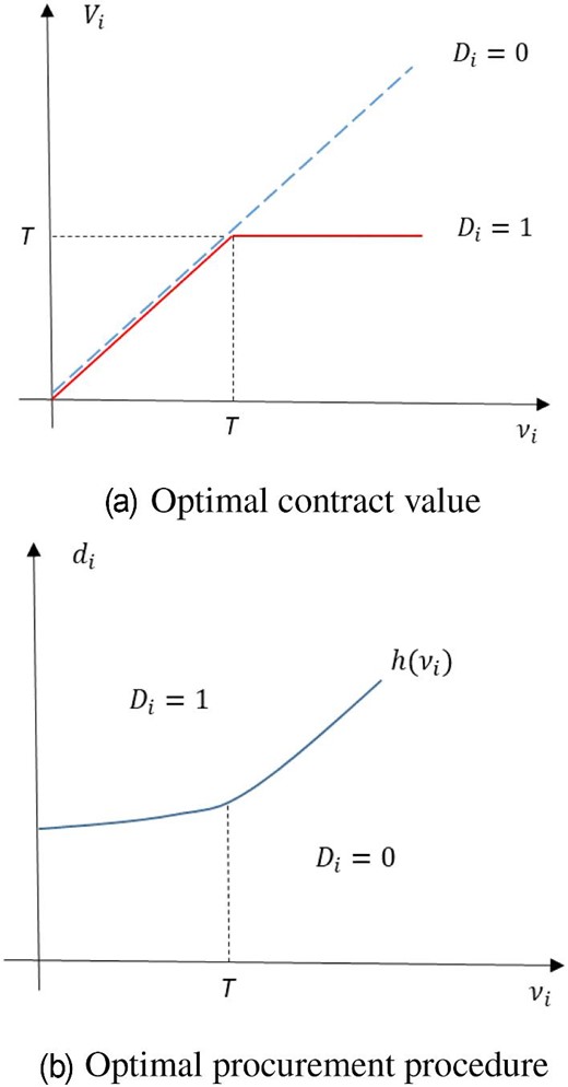
Optimal choices in Regime 2.
Figure 5(b) illustrates the agency’s procedure decision. She chooses a high-discretion procedure if the latent benefit of high discretion |$d_i$| is larger than the critical value |$h(\nu _i)$|. This budget (or project size) specific critical value captures two things. First, it formalizes the idea that procuring agencies may have different sensitivity to administrative costs or procurement outcomes for large contracts from that for small contracts. For example, an increasing h could mean that agencies are willing to pay the larger administrative costs of an auction only if the project is sufficiently large. Second, h also captures the extra cost of fitting contract value below the procurement threshold—either by manipulating the list price or reducing the quantity—for projects with budgets larger than the threshold. Since this extra cost is increasing in the size of the contract value distortion, then the slope of h becomes larger above the procurement threshold.
In the next two sections, I outline both a nonparametric and a parametric empirical strategy to estimate the budget specific critical values |$h(\nu _i)$| and use it to disentangle the effect of discretion from the impact of sorting.
4.3. Semi-Parametric Estimation
This section combines the model of the previous section and the difference-in-differences variation of the procurement reform. Since the focus of this section is to correct for possible sorting of tenders into the high-discretion procedure, I keep the agency’s demand for discretion as general as possible and estimate it nonparametrically.
To estimate parameters of equation (2), I assume it takes a more specific form
where |$\delta$| captures the causal effect of discretion, |$f(V_i)$| is an arbitrary function of the anticipated contract value,15 and |$\textit{Post}_{i}$| is an indicator for the post-reform period capturing time effects in procurement outcomes. The residual has two components: |$u_i$| and |$\xi _i$|, where the former is only observed by the procuring agency but not by the econometrician, while the latter is unobservable to both.
As we have seen in Section 3, the main empirical challenge lies in the endogeneity of procedural decisions. Since the procuring agency controls the procurement procedure, then |$D_{i}$| may be correlated with the outcome-relevant heterogeneity observed by the agency (captured by |$u_i$|), which renders the OLS estimate of |$\delta$| inconsistent.
I address the problem of self-selection into the high-discretion procedure by estimating equation (5) together with the selection equations implied by the procurement model of the previous section. Proposition 1 implies selection equations both on the procedure and on the contract value
To allow for a nonparametric estimation of |$h(\nu _i)$|, I assume that the budget |$\nu _i$| has a discrete support, |$\nu _{i}\in \left\lbrace v_{1},\ldots ,v_{N} \right\rbrace$|, and I discretize the reported contract value using the same bins. I also assume that |$\nu _{i}$| is independent of both |$u_i$| and |$d_i$|.16 It is important to notice that the independence of |$\nu _i$| and |$d_i$| is not a very restrictive assumption since the project size can still influence the utility gain from discretion through the budget specific critical value |$h(\nu _i)$|.17 As a result, the assumption does not rule out that an agency benefits more from high discretion in large than in small contracts.
Finally, I assume that |$\xi _i$| is independent from everything, but |$\epsilon _{i}$| and |$u_{i}$| are jointly normally distributed with expected values of zero and variance
This assumption implies that d and u are also normally distributed.18 Since we cannot identify both |$h(\nu _i)$| and |$\sigma _d$| at the same time, I normalize |$\sigma _d \equiv 1$|. The correlation between u and d (|$\rho _{u,d}$|) formalizes the key idea that tenders sort into the high-discretion procedure based on their unobserved characteristics. The distributional assumption—joint normality of |$\epsilon _i$| and |$u_i$|—is not crucial to the identification of the model but it increases statistical power. In Section A3.1, I report estimates relaxing the distributional assumption and find very similar results.
Given this data generating process, equation (5) can be written as
where |$CF(D_i, V_i, {\mathit Post}_i)$| is a control function capturing the selection into the high-discretion procedure, and it is given by19
After the inclusion of the control function, discretion in equation (8) is no longer endogenous, formally |$E[\eta _i|V_i,D_i,{\mathit Post}_i,CF_i]=0$|.
To construct the control function given by equation (9), we need to estimate the budget specific critical values |$h(\nu _i)$|. In order to do so, notice that:
Since |$\Phi ^{-1}$| is a monotonic function, the probability of an open auction conditional on the budget in the post-reform period |$\Pr (D_i=0|\nu _i, {\mathit Post}_i =1)$| carries the same information as |$h(\nu _i)$|. If the budget is below the threshold, therefore it is equal to the reported value, then the probability of an open auction is directly observable. Formally it is given by
However, if the budget is above the threshold, then the probability of an open auction is no longer directly observable since high-discretion tenders bunch below the threshold. The key idea of the identification strategy is that the post-reform budget distribution is similar to the pre-reform contract value distribution, thus the latter provides a good counterfactual for the post-period contract value distribution in the absence of bunching. This assumption allows us to quantify the probability of an open auction conditional on budgets above the threshold by calculating the missing mass relative to the pre-reform period. Formally,
Estimation.
Following Heckman (1979), I estimate the model in two steps. First, for each grid of the discretized contract value I estimate |$\Pr (D_i=0|\nu _i, {\mathit Post}_i=1 )$| nonparametrically by using equations (10) and (11) and construct the control function by substituting the probabilities into equation (9). Second, I estimate equation (8) by OLS.
It is important to notice that the excluded instruments of this two-stage procedure are the interaction terms of the budget and the post-reform indicator, since I estimate a fully saturated model of |$\nu _i$| and |${\mathit Post}_i$| in the first stage but their effects are additively separable in the second stage. The exclusion restriction relies on the assumption that function |$f(\cdot )$| in equation (5) is time-invariant. It captures the idea that the time effect is uniform across all contract values, and any value specific change over time enters equation (8) through the control function.
Identification.
Figure 6 illustrates the logic of the identification. Figure 6(a) plots, separately for the pre- and post-reform period, the log-TFP of open auction winners as a function of contract value. The difference between the outcomes over time is driven by two forces: the time effect (|$\tau$|) and the sorting induced change in the composition of tenders across time periods (|$\rho _{u,d}$|). The time invariance of |$f(\cdot )$| in equation (5) implies that, in the absence of sorting, the log-productivity curve of open auctions is unique up to parallel shifts. However, sorting can transform the shape of the curve over time as different points of the value distribution are exposed to varying degrees of sorting in the post-reform period. Indeed, below the threshold where the discretionary procedure is easily available, the composition of tenders has changed markedly between the pre- and post-reform periods. However, the further the budget is above the threshold, the more contract value agencies need to sacrifice to gain high discretion. Therefore, as we move further from the threshold, the difference in the composition of tenders between the pre- and post-periods becomes smaller, which explains the closing gap between the two curves. As a result of this, the comparison of outcomes displayed in Figure 6(a) identifies the effect of sorting.
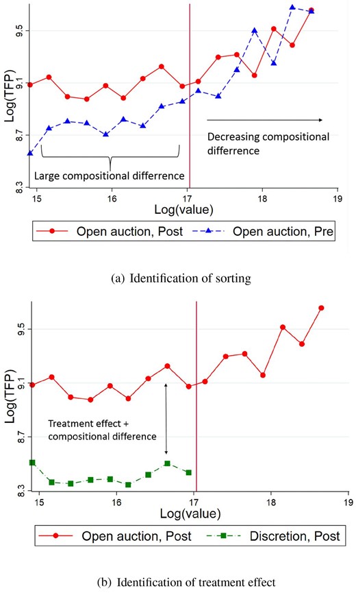
Identification of the model.
Once we know the effect of sorting, we can compare the outcomes of different procedures to identify the treatment effect of discretion. This comparison is illustrated in Figure 6(b), which plots the log-productivity of open auctions and high-discretion procedures in the post-reform period. The difference between the outcomes of open auctions and high-discretion procedures is given by the sum of the sorting and the treatment effect. Therefore, we can identify discretion’s effect by partialling out the known impact of sorting. Notice that the causal effect is local to smaller contracts, since we can only compare contracts below the value threshold.
4.4. Parametric Estimation
The semi-parametric approach of the previous section corrected for sorting by estimating the agency’s demand for discretion nonparametrically. The main advantage of that approach is that it does not impose any functional form assumption on the utility function and consequently on the budget specific critical value |$h(\nu _i)$|. However, the non-parametric approach has two major limitations. First, it does not allow us to investigate the determinants of the demand for discretion. Second, it does not explicitly identify the trade-off between choosing the high-discretion procedure and the optimal contract value (which agency faces if the budget exceeds the threshold), therefore it does not allow us to explore the consequences of alternative thresholds.
In this section, I propose a fully parametric approach, which—at the expense of more assumptions—helps me to overcome these shortcomings and estimate the determinants of the demand as well as the trade-off between discretion and contract value.
In order to estimate the demand for discretion parametrically, I assume that the agency’s utility, given by equation (4), takes a more specific form
This utility function is the sum of two terms. The first term is only a function of the anticipated contract value. The second term, which captures the extra utility from discretion, depends on observable tender characteristics |$X_i$|, outcome-relevant tender characteristics observed only by the procurer |$u_i$|, and the administrative cost advantage of high discretion |$\epsilon _i$|. Observable tender characteristics may include the type of the procuring agency (central versus local governmental agency), some proxy for product complexity, and other factors driving the agency’s demand for discretion, such as the share of domestic or connected firms in the product’s market.
Since this utility is a specific example of equation (4), it has to be an increasing function of |$V_i$| (it is implied by the combination of Assumptions 1 and 2) and satisfy Assumption 3. Monotonicity is easy to see as |$\log V_i$| is an increasing function of the contract value. The utility gain from choosing high discretion is linear, therefore continuous and strictly monotonic, in |$d(\epsilon _i,u_i) \equiv \varphi u_i + \epsilon _i$|, which satisfies Assumption 3.
In this setup, the optimal contract value, given by equation (7), remains the same as in the semi-parametric analysis presented above, but outcome equation (5) modifies to
which also includes observable tender characteristics |$X_i$|. Similarly to equation (5), the residual has two components |$\mu _i \equiv u_i + \xi _i$|, where |$u_i$| is only observed by the agency but is unobservable to the econometrician and |$\xi _i$| is unobservable to everyone.
As a result of the parametric utility in equation (12), the procedure selection equation also takes a more specific form
where the non-parametric |$h(\nu _i)$| function of the previous section is replaced by a parametric function of |$X_i$|, |$\nu _i$| and T.
I assume that |$\xi _i$| is normally distributed and independent from everything and |$\epsilon _i$| and |$u_i$| are jointly normally distributed, which implies that |$(\mu _i, d_i)$| is also normal. Just like |$\rho _{u,d}$| in the previous section, |$\rho _{\mu ,d}$| captures sorting based on unobservables. However, unlike in the previous section, I include a richer set of controls into equation (13), which allows me to explain part of the sorting with observables. Also, now I can identify |$\sigma _d$|, which captures the sensitivity of the procedure choice to unobservables.
Similarly to the previous section, I assume that |$\nu _{i}$| and |$V_i$| have the same discrete support |$\lbrace v_1,...,v_N\rbrace$|, with probability weights |$\lbrace \Pr (\nu _i = v_{j})\equiv q_{j}\rbrace ^N_{j=1}$|. The budget |$\nu _{i}$| is independent from |$d_{i}$| and |$\mu _{i}$| and I approximate |$f(V_i)$| with a third-order polynomial of |$\log V_i$|.
The vector of parameters |$\theta$| consists of (i) the parameters of tender characteristics in the selection equation |$\eta$|; (ii) discretion’s effect on the outcome |$\delta$|, the parameters of tender characteristics in the outcome equation |$\gamma$|, the parameters of the |$\widehat{f}(V_i)$| function, and the time effect |$\tau$|; (iii) the parameters of the variance-covariance matrix of |$\mu _i$| and |$d_i$| (|$\sigma _\mu$|, |$\sigma _d$|, and |$\rho _{\mu ,d}$|); and (iv) the probability weights of the budget space |$\lbrace q_{j}\rbrace ^{N}_{j=1}$|. I estimate the parameter vector |$\theta$| with maximum likelihood method.
The likelihood of an observation from the pre-reform period is
where |$\widehat{\mu }_i$| is the predicted residual of equation (13) and |$g_{\mu }$| is the pdf of this residual. If the contract was awarded in the post-reform period then the likelihood is
where |$G_{d|\mu }(\cdot )$| is the cdf of |$d_i|\mu _i$|. I estimate the parameter vector |$\theta$| which maximizes the likelihood function20
This approach has two important advantages. First, by identifying utility parameters, it measures the associations between tender characteristics and the demand for discretion expressed in terms of foregone contract value. Namely, we answer the question of how much more contract value agencies are willing to sacrifice—when the budget is above the threshold—to gain discretion if we increase |$X_i$| by one unit. Second, since it explicitly identifies the trade-off between discretion and contract value, it allows for the simulation of the effects of counterfactual thresholds on the distribution of contract values and on average procurement outcomes.
Identification.
The identification of the causal effect of discretion and the sorting of tenders into the high-discretion procedure is based on the same idea as in the semi-parametric approach. It exploits the time variation of the reform and the assumption that the distribution of the pre-reform period is a good counterfactual for the post-reform period.
The novelty of the parametric approach is the explicit identification of the trade-off between discretion and contract value and its associations with tender characteristics. We can evaluate the importance of high discretion in terms of forgone contract value by analyzing the gap between the right tales of the contract value distributions of the pre- and post-reform periods. If this gap closes fast, then agencies are sensitive to reductions in contract value. Conversely, if the gap closes slowly, then agencies are willing to sacrifice more contract value to get discretion. The difference of this gap across contracts with different characteristics identifies the |$\eta$| parameters of the selection equation.
5. Results
5.1. Main results
Table 2 presents my baseline results using the non-parametric selection correction procedure. The table reports the effects of discretion on three groups of outcomes: competition, contractor’s productivity, and political favoritism. Panel A shows the naive OLS regressions while Panel B presents the selection correction specifications, which control for the sorting of tenders by including the control function described in the previous section. Column (1) reports results on the logarithm of the normalized price. After controlling for selection, discretion increases prices by 6.4 percentage points, which is slightly larger than the correlation detected by the naive OLS, but somewhat smaller than the RDD result. However, results on normalized prices should be interpreted with caution because the manipulation of list prices—to fit reported value below the threshold—creates a mechanical positive correlation between discretion and the normalized price. To investigate this concern, I build on the assumption—supported by both Figure 2 and the model—that contracts with manipulated list prices are clustered right below the threshold. In Section A3.2, I re-estimate the baseline specifications omitting observations of the bin below the threshold. Column (2) confirms discretion’s negative impact on competition by reporting that it reduces the number of bidders by almost one.21
Discretion’s effect on procurement outcomes.
| Connection of the winner firm | ||||||
|---|---|---|---|---|---|---|
| Log(norm price) | No. of bidders | Log(TFP) | Right | Left | Unconnected | |
| (1) | (2) | (3) | (4) | (5) | (6) | |
| Panel A: Naive OLS | ||||||
| Discretion | 0.055 | −0.739 | −0.636 | 0.091 | 0.014 | −0.026 |
| (0.009) | (0.097) | (0.067) | (0.014) | (0.006) | (0.021) | |
| Post period | −0.007 | 0.191 | 0.184 | −0.026 | −0.022 | −0.009 |
| (0.008) | (0.103) | (0.056) | (0.010) | (0.007) | (0.019) | |
| Panel B: Selection correction | ||||||
| Discretion | 0.064 | −0.954 | −0.282 | 0.108 | 0.027 | 0.031 |
| (0.019) | (0.190) | (0.135) | (0.039) | (0.016) | (0.051) | |
| Post period | −0.013 | 0.316 | −0.006 | −0.033 | −0.026 | −0.031 |
| (0.013) | (0.117) | (0.083) | (0.019) | (0.007) | (0.024) | |
| Control fn | −0.006 | −0.138 | −0.229 | −0.012 | −0.008 | −0.039 |
| (0.011) | (0.126) | (0.086) | (0.024) | (0.011) | (0.036) | |
| Mean of dep. var. for open auctions | −0.130 | 2.95 | 9.06 | 0.078 | 0.025 | 0.476 |
| Observations | 44,915 | 47,971 | 34,930 | 12,249 | 12,249 | 12,249 |
Notes: Each observation is an individual contract. The sample consists of non-construction tenders for 2009–2015. Columns (4)–(6) are restricted to tenders with at least one top 500 bidder. The dependent variables are the log-ratio of the winning bid and the anticipated contract value in column (1), number of bidders in column (2), log-TFP of the winning firm in column (3), and indicators for the winning firm being right-, left-, or unconnected in columns (4)–(6). Panel A reports naive OLS specifications and Panel B reports results of the second step of the selection correction model. Each specification also includes a cubic function of the log-anticipated contract value. Bootstrapped standard errors clustered by the procuring agency in parentheses.
Column (3) shows that discretion results in the selection of 28% less productive contractors. This effect is only a third of the correlation presented in Panel A (and also of the RDD result), which implies that the sorting of low-productivity tenders—tenders in which the winner firms’ productivity would have been low even if open auctions had been used—accounts for two-thirds of the raw correlation between discretion and the contractor’s productivity.22
The last block documents discretion’s impact on the political connections of the selected contractor. Column (4) shows that, with a causal effect of 11 percentage points, discretion more than doubles right-connected firms chance of winning the award. This effect slightly exceeds the correlation in panel A, but is somewhat smaller than the RDD result. Column (5) reports that discretion has some effect—about a quarter of the effect on right connected firms—on the winning chances of firms connected to the left. Despite being small, this is a meaningful effect (relative to the small baseline chance of left-connected contractors), which may indicate some rent-sharing between political parties or unobserved connections to the right. Unlike connected companies, column (5) reports small (relative to the baseline outcome) and insignificant effects on unconnected firms.
The main results presented in Table 2 prove that the large differences in allocations detected by the RDD are not entirely driven by the sorting of tenders but also by the true causal effect of discretion. To put it differently, with more discretion at hand agencies pay more for the same anticipated value and select less productive but more connected contractors.
The effects are very similar across different product categories and levels of government. This is confirmed by Online Appendix Table A7, which investigates treatment effect heterogeneity.
General Equilibrium Effects.
Given large effects documented by Table 2, one might expect that increased buyers’ discretion has a spillover effect on other tenders as well. Indeed, by restricting the access of unfavored companies to high-discretion tenders the policy reform may have increased competition in the remaining low-discretion tenders. Online Appendix Figure A3 investigates this by plotting the average number of bidders in open auctions over time. The figure finds that the reform had no clear effect on the number of bidders in open auctions, which suggests that the spillover effect on low-discretion tenders is limited.
5.2. Robustness
Here, I present some robustness tests on the baseline results.
Identifying Assumptions.
The structural model builds on three important assumptions: (i) the pre-reform contract value distribution provides a good counterfactual for the post-reform distribution in the absence of bunching; (ii) there are no contract value specific time effects in equation (5), meaning that function |$f(V_i)$| is the same in the pre- and the post-reform periods; and (iii) administrative costs |$\epsilon _{i}$| and outcome-relevant unobserved heterogeneity |$u_{i}$| are jointly normally distributed.
Section A3.1 in the Online Appendix tests the validity of these assumptions. First, to investigate the robustness of my results to the counterfactual value distribution, I create an alternative counterfactual—following Carril (2021)—by combining a bunching estimator with time variation in the value distribution. Online Appendix Table A3 reports the results using this alternative counterfactual and confirms the findings of Table 2. Second, in Online Appendix Figure A6, I provide direct evidence on the stability of function |$f(V_i)$|. Third, I jointly test the validity of assumptions (i) and (ii) by narrowing the time window around the policy change, which makes any continuous change less pronounced.23 Online Appendix Table A4 presents the results of the main specifications using data from different time windows around the policy change. Although some point estimates are smaller in absolute terms, all results remain qualitatively unchanged. Finally, I test the robustness of assumption (iii). Since the identification relies on the difference-in-differences variation of contracts (high discretion became available only below the threshold in the post-reform period), this assumption is not essential to the identification of the effect of sorting. I can relax this assumption by approximating the unknown functional form of the control function with a polynomial of the probability of using an open auction. Online Appendix Table A5 reports the estimates without the distributional assumption and confirms the findings of the main specification of Table 2.
Manipulated List Price.
Agencies can reduce reported value—to fit it below the threshold—by decreasing quantity and (or) by manipulating the list price. Unlike quantity distortions, the manipulation of list prices constitutes a major risk to the identification of discretion’s effect on log-normalized prices. It creates an endogeneity problem that goes beyond the unobserved heterogeneity based sorting of contracts—which makes |${\mathit Corr}(D_i,u_i) \ne 0$|—because it adds the new component |$w_i$| to the residual of equation (5),
where |$w_i \equiv \log \bar{p}_i - \log p_i$|.
If an agency uses a smaller list price to fit the reported value below the threshold, then the new residual |$w_i$| becomes positive. In this case, |${\mathit Corr}(D_i,w_i)>0$|, so the manipulation of the list price creates a mechanical positive relationship between discretion and the observed normalized price. Fortunately, both the model and the location of the excess mass on Figure 2 help us to identify observations with manipulated prices. Since there is no incentive to manipulate list prices if |$p_i q_i \ne T$|, then most, if not all, manipulated observations cluster right below the threshold. Although it is true that list price manipulation affects the composition of contracts above the threshold as well, but that is captured by the correlation of |$u_i$| and |$D_i$|, which the control function aims to deal with. This implies that the exclusion of observations in the bin below the threshold substantially reduce the size of the problem.
Online Appendix Table A8 reports results of the specification excluding the bin below the threshold. All results are very similar to the ones reported in Table 2 confirming that the baseline results are not driven by observations with manipulated list prices.
Different Productivity Measures.
In Table 2, I use a productivity measure developed by Wooldridge (2009) to account for firm-level unobservables in the estimation of the production function. Nevertheless, to test whether the main results depend on the specific measure of productivity, Online Appendix Table A9 reports estimates using alternative productivity measures. The results, although somewhat smaller in absolute size, are consistent with the main specification.
Markups.
All measures of productivity I use in this paper are based on the revenue of the firm, therefore they conflate the effects on physical productivity with those on markups. Online Appendix Table A10 explores whether discretion’s impact on measured productivity is really driven by its effect on physical productivity. Column (1) reports estimates on the markup as an outcome. As before, Panel A shows the naive OLS and Panel B the estimates of the selection correction model. The latter finds an insignificant effect of discretion on markups. Columns (2)–(4) perform a mediation analysis and re-estimate discretion’s effect on different measures of productivity controlling for the markup of the winner firm to close down the causal channel though markups. Results are essentially the same as the baseline confirming that discretion’s effect operates through physical productivity.
Flexible Functional Form.
The baseline specifications approximate |$f(V_i)$| in equation (5) with a cubic function of the log-value. I validate this functional form assumption by replacing the cubic with a non-parametric function of the contract value.24 Online Appendix Table A11 reports very similar results to my baseline findings underscoring the insensitivity of the main results to functional form assumptions.
5.3. Mechanisms
The previous sections documented that bureaucratic discretion has a great influence on procurement outcomes. Beyond reducing competition and increasing prices, it allows agencies to favor a different set of contractors, who are less productive but more likely to be connected to the governing party. A straightforward interpretation of this finding is that the change in allocations is driven by the private interests of bureaucrats and politicians and less productive companies are favored because they have political connections. Online Appendix Table A12 provide some additional support to this interpretation by documenting that discretion has a stronger negative effect on competition and contractor productivity in product categories in which more connected firms operate.25
However, connections are, of course, endogenous. While I can isolate the causal effect of discretion on who wins the contract, firms favored by procuring officials are certainly not only different in their connections or productivity. In principle, there could be numerous public benefits of awarding contracts to less productive firms. I test for several potential benefits, and find no evidence for them.
5.3.1. Contract Execution
A major caveat of the approach focusing on ex-ante outcomes is that they do not measure the quality of contract execution. Indeed, ex-ante measures of contractor quality may be negatively correlated with ex-post measures of contract execution if agencies choose less productive contractors because they have relation specific expertise or better incentives to execute contracts properly—Section 5.3.3 investigates evidence on these mechanisms in more detail. Similarly, if auctions are won by unrealistically low bids, which are hard to enforce, then low ex-ante prices may not necessarily translate into low ex-post prices. To overcome these challenges, the standard approach in the procurement literature is to use proxies of contract execution, such as post-award contract modifications, delays in delivery, and cost overrun (Coviello, Guglielmo, and Spagnolo 2017; Carril 2021). Using data created by Fazekas, Tóth, and King (2016), for a subset of contracts in the pre-reform period, I have access to similar measures of contract execution. Unfortunately, since data is limited to the pre-reform period I can not employ my main specification to analyze the relationship between discretion and contract execution, but I can use the data to study associations between ex-ante and ex-post procurement outcomes.
Table 3 presents partial correlations26 between ex-ante measures of quality (contractor productivity and normalized price) and various ex-post execution measures: (i) an indicator for post award contract modifications, (ii) delays in delivery in days, and (iii) logarithm of the normalized ex-post price—measured by the log-ratio of the ex-post price and the anticipated contract value. My results suggest a positive link between the productivity of the contractor and the quality of contract execution. Indeed, higher contractor productivity is associated with less post award contract modifications and is uncorrelated with delays and ex-post prices. The normalized price seems unrelated to measures of contract execution, such as contract modifications and delays. However, there is a strong positive correlation between ex-ante and ex-post prices. Column (3) suggests that although cost overruns are more frequent in contracts where the winning bid was low, the ex-ante price is still a good proxy for the ex-post acquisition cost.
Measures of contract execution.
| Contract modified | Delay | log(ex-post price) | |
|---|---|---|---|
| (1) | (2) | (3) | |
| Log(TFP) | −0.010 | 0.612 | −0.004 |
| (0.002) | (2.40) | (0.015) | |
| Log(norm price) | −0.0004 | 5.24 | 0.433 |
| (0.009) | (6.36) | (0.074) | |
| Mean of dependent variables | 0.178 | −4.48 | −0.085 |
| Observations | 14,720 | 4,757 | 4,120 |
Notes: Each observation is an individual contract. The sample consists of tenders for 2009–2012. Each specification includes a cubic function of the log-anticipated contract value, procuring agency and year fixed effects. Standard errors clustered by procuring agency in parentheses.
5.3.2. Domestic and Local Contractors
Government agencies may use discretion to stimulate the local economy by favoring local or domestic firms—which are less productive and more connected but employ more workers locally. Indeed, many countries have explicit rules helping small, domestic, or disadvantaged firms in becoming government contractors (see Rosa 2020). European law forbids the explicit discrimination of companies from other EU countries but the high-discretion procedure may create an opportunity to tilt the playing field in favor of domestic companies. Columns (1)–(3) of Table 4 investigate this hypothesis and provides no support for it. Similarly to Table 2, Panel A reports the naive OLS results, while Panel B controls for the sorting of tenders. Panel A finds strong correlations between discretion and both the size and the domestic ownership of the company. However, the effects reported in Panel B fall short of the correlations. Discretion has basically no effect on domestic ownership and a limited effect—a 9% decrease—on the number of employees. Similarly, Panel B of column (3) estimates an economically small and insignificant effect—about a 6.5 km reduction—on the distance between the requestor agency and the contractor’s HQ suggesting that local firms do not benefit substantially from the high-discretion procedure.
Discretion’s effect on other contractor characteristics.
| Domestic | Log(emp) | Distance | Experienced | Incumbent | Firm age | Exit | |
|---|---|---|---|---|---|---|---|
| (1) | (2) | (3) | (4) | (5) | (6) | (7) | |
| Panel A: naive OLS | |||||||
| Discretion | 0.095 | |$-0.836$| | |$-9.16$| | |$-0.128$| | |$-0.225$| | |$-3.14$| | 0.015 |
| (0.013) | (0.048) | (4.02) | (0.010) | (0.019) | (0.210) | (0.008) | |
| Post reform | 0.002 | 0.214 | 0.763 | 0.174 | 0.191 | 2.79 | 0.005 |
| (0.013) | (0.047) | (3.71) | (0.011) | (0.020) | (0.222) | (0.006) | |
| Panel B: selection correction | |||||||
| Discretion | |$-0.015$| | |$-0.125$| | |$-6.48$| | |$-0.091$| | |$-0.203$| | |$-0.867$| | 0.040 |
| (0.028) | (0.129) | (5.82) | (0.029) | (0.039) | (0.654) | (0.018) | |
| Post reform | 0.066 | |$-0.198$| | |$-8.22$| | 0.153 | 0.178 | 1.46 | |$-0.010$| |
| (0.019) | (0.084) | (4.34) | (0.019) | (0.025) | (0.472) | (0.012) | |
| Control fn | 0.071 | |$-0.456$| | |$-10.0$| | |$-0.024$| | |$-0.014$| | |$-1.45$| | |$-0.016$| |
| (0.018) | (0.085) | (4.21) | (0.020) | (0.021) | (0.379) | (0.012) | |
| Mean of dep. var. for open auctions | 0.805 | 3.25 | 68.4 | 0.703 | 0.332 | 15.1 | 0.057 |
| Observations | 40,352 | 40,143 | 37,730 | 48,380 | 48,380 | 41,616 | 41,342 |
Notes: Each observation is an individual contract. The sample consists of non-construction tenders for 2009–2015. The dependent variables are an indicator for domestically owned contractors in column (1), log-employment of the contractor in column (2), the distance (in km) of the requesting agency and the contractor’s HQ in column (3), an indicator for non-first time procurement winners in column (4), an indicator for incumbent winners (which won contracts from the same agency-product category pair before) in column (5), the age of the contractor in column (6), and an indicator for firm exit in the 3-year window after the contract. Panel A reports naive OLS specifications and Panel B reports results of the second step of the selection correction model. Each specification also includes a cubic function of the log-anticipated contract value and an indicator for the post-reform period. Bootstrapped standard errors in parentheses.
Online Appendix Table A13 provides further evidence against this mechanism by investigating political favoritism in domestic intensive product categories. In these product categories, contractors are predominantly domestic even if they were chosen in open auctions.27 The results suggest that right-connected firms enjoy an even larger premium in domestic intensive product categories. However, results for left- and unconnected firms are unchanged. This finding speaks against the claim that political favoritism is only the side effect of agencies’ preference for domestic contractors.
5.3.3. Match Quality and Relational Contracts
Discretion can also serve taxpayers’ interests by improving the match between agencies and contractors. Indeed, if discretion helps agencies to favor firms specialized on the specific needs of public buyers, then it can improve unobserved product quality. Although match quality is unobservable, column (4) of Table 4 may provide some indirect evidence by exploring contractors previous experience with public buyers. Surprisingly, column (4) shows that discretion increases the probability of first time government suppliers. This finding makes a positive impact on match quality less likely.
An important literature highlights that discretion may create better incentives for contract execution by allowing relational contracts. Under these contracts, procurers may favor incumbent winners in order to keep them motivated by the future value of the relationship. Indeed, Coviello, Guglielmo, and Spagnolo (2017) find that discretion benefits incumbent firms in Italy. Column (5) of Table 4 investigates the same question but finds opposite results. In Panel B, discretion decreases the probability of an incumbent winner by 18 percentage points. This result seriously questions that discretion promotes the use of relational contracts. Although it is important to keep in mind that high-discretion procedure became widely available only in the post-reform period. Therefore, many of the incumbent winners are firms, which had previously won contracts in open auctions.
The evidence above speaks against improvements of match quality and relational contracts but it seems to be in line with journalistic accounts of political favoritism. Bruckner (2017) and Rényi (2018) argue that politically connected entrepreneurs use complicated ownership structures and short lived companies to avoid detection. Indeed, the use of project companies which are closed after one or just a few projects makes it harder for media outlets to track systematic political favoritism. The high turnover among politically favored companies may contribute to the negative effect on the winning chances of experienced and incumbent firms. Columns (6) and (7) of Table 4 provide direct evidence on the shorter lifespan of contractors selected in high-discretion procedures. Column (6) shows that companies selected in high-discretion procedures are somewhat younger and column (7) reports a positive effect on contractor firms’ exit rate in the 3 years after the contract decision.28 The higher exit rate is not only an evidence of shorter lifespan but it is generally a negative signal about firm quality.
5.4. Results of the Parametric Estimation
In this section, I discuss the results of the parametric estimation. Similarly to the semi-parametric approach, the parametric model identifies the effects of discretion on procurement outcomes but it also identifies the demand for the discretionary procedure as a function of tender characteristics and the procurement threshold. This is useful in two ways: (1) it sheds some light on the associations between tender characteristics and the demand for discretion and (2) it allows us to explore the consequences of counterfactual procurement policies.
There are multiple tender characteristics that may influence agencies’ procedural decisions. If political favoritism was an important driver of the demand for discretion, then we would expect agencies to choose discretion more often in product categories where more connected firms operate. I investigate this question by estimating the association between the demand for discretion and the share of connected firms in a market.29 Since the connected firms are much larger than the average contractor I also include the share of unconnected top 500 firms as a benchmark. Similarly, agencies may choose discretion to favor domestic firms, which would translate into a positive correlation between discretion and the share of domestic firms in the market.30 The type of the procuring agency can also shape procedure preferences since central government agencies may have more administrative capacity to organize auctions than local governments. Finally, contract theory suggests that auction is more costly for complex products, where including all details in the contract is difficult. Services are arguably more complex and more costly to contract than goods, so we may expect a stronger demand for discretion in the purchase of services than that in the purchase of goods.
Table 5 presents the results of the parametric estimations. Columns (1) and (2) report the results of the specification using log-normalized price as the dependent variable of equation (13). Column (1) shows the parameter estimates of the procedure selection equation, while column (2) shows the estimates of the outcome equation. Columns (3) and (4) present similar results using the contractor’s log-TFP as the dependent variable of the outcome equation. Results in columns (1) and (3) are different because the same selection equation is estimated on different samples.31
Parametric estimation results.
| Price | Productivity | ||||
|---|---|---|---|---|---|
| Discretion | Log(norm price) | Discretion | Log(TFP) | ||
| (1) | (2) | (3) | (4) | ||
| Discretion | 0.056 | |$-0.289$| | |||
| (0.018) | (0.221) | ||||
| Share of connected top 500 firms | 0.873 | 0.034 | 0.577 | 8.90 | |
| (0.154) | (0.018) | (0.179) | (0.119) | ||
| Share of unconnected top 500 firms | |$-0.349$| | |$-0.045$| | |$-0.428$| | 1.39 | |
| (0.062) | (0.008) | (0.077) | (0.054) | ||
| Share of domestic firms | 0.300 | |$-0.058$| | 0.224 | |$-2.33$| | |
| (0.060) | (0.008) | (0.069) | (0.052) | ||
| Central government agency | |$-0.640$| | |$-0.014$| | |$-0.566$| | 0.098 | |
| (0.031) | (0.004) | (0.033) | (0.031) | ||
| Services | 0.707 | |$-0.042$| | 0.573 | |$-0.669$| | |
| (0.031) | (0.004) | (0.032) | (0.031) | ||
| Correlation of d and μ | 0.026 | -0.111 | |||
| (0.046) | (0.098) | ||||
| Observations | 44,915 | 34,930 | |||
Note: Each observation is an individual contract. The sample consists of non-construction tenders for 2009–2015. Columns (1) and (2) (columns 3 and 4) report the results of the parametric model using log-normalized price (log-TFP) as the dependent variable of the outcome equation. Odd columns report the parameter estimates of the selection equation, while even columns report them for the outcome equations. Share of connected top 500 firms is the share of total contract value awarded to right-connected top 500 firms during the pre-reform period in the tender’s product category, Share of unconnected top 500 firms and Share of domestic firms are corresponding shares for firms unconnected to the right and for domestic companies. The outcome equations also include a cubic function of log-anticipated contract value and an indicator for the post-reform period, which are not reported in the table. Standard errors in parentheses.
As we can see in column (1) and (3), as the share of connected companies increases by 1 percentage point, agencies are willing to sacrifice 0.6%–0.9% more contract value to get discretion. Although I control for a few key tender characteristics, which may be correlated with the connected share (e.g., services indicator and domestic share), in the absence of exogenous variation in the connected share this finding does not necessarily capture a causal relationship. However, the share of unconnected top 500 firms—which are similar to the right-connected top 500 firms in many observables—is negatively associated with the demand for discretion suggesting that the connections of these firms matter. Similarly to connected firms there is a positive correlation between discretion and the share of domestic companies in the market. Not surprisingly, columns (1) and (3) document that local governments and agencies buying services choose discretion more often, which is consistent with the findings of Baranek and Titl (2020).
The effects of discretion on the outcomes, reported in columns (2) and (4), are very similar to the semi-parametric estimates discussed in the previous section. The results on the sorting of tenders are also in line with the semi-parametric estimates of the previous section. The combination of columns (1) and (2)—focusing on the log-normalized price—suggest that the sorting of tenders based on observable tender characteristics is ambiguous. To put it differently, it is not immediately clear whether agencies of low- or high-price tenders choose discretion more often. Firm connections and the type of the agency imply the sorting of high-price, while the share of domestic companies and the sector of the product imply the sorting of low-price tenders. The small and insignificant correlation between u and d indicates a limited sorting based on unobservables. On the other hand, columns (3) and (4)—focusing on log-TFP—document the sorting of low-productivity tenders based on both observables and unobservables. All tender characteristics—with the exception of the share of connected firms—imply that agencies choose discretion more often in tenders where the contractor’s productivity would be low anyway. Also, the negative correlation between μ and d in column (4) implies a sorting of low productivity tenders driven by unobservables.32 Nevertheless, this sorting based on unobservables is smaller then the one detected by the semi-parametric estimates because a big part of the sorting is explained by observable tender characteristics such as domestic share, agency type, and the sector of the good.
6. Policy Simulations
In this section, I use the structural results of Section 5.4 to conduct policy simulations. First, I quantify the impacts of numerous procurement thresholds—among them the actual threshold introduced in 2011—relative to the benchmark policy of requiring open auctions for all contract values (which is equivalent to a threshold of zero forints). Second, I investigate how regulatory oversight interact with procurement thresholds. I simulate the impacts of thresholds both under the estimated and under a high level of scrutiny—where the high level of scrutiny prevents agencies from distorting procurement value for more discretion.
The parametric model helps us to explore the consequences of different procurement policies by explicitly linking agencies’ value and procedure decisions to the procurement threshold. More specifically, it allows us to simulate the effect of counterfactual thresholds and levels of scrutiny both on the value and on the outcome of each individual contract. Combining these two, we can compute the effect of any threshold and scrutiny combination on the value weighted average outcome relative to the zero threshold benchmark:
where |$Y_i(T,s)$| is the outcome of interest—normalized price or the contractor’s TFP—and |$V_i(T,s)$| is the approximated value of contract i for threshold T and scrutiny level s.
The model highlights that increasing the threshold affects procurement outcomes through two different channels. First, it affects them directly by making the discretionary procedure more widely available, which increases the price and reduces the contractor’s TFP. The second effect roots in the threshold-induced distortion of the contract value distribution. The high-discretion procedure is only available for contract values below the threshold, creating a sorting of contracts from larger auctions to smaller discretionary tenders. Since this sorting is not random but is based on observable and unobservable tender characteristics, the bunching of tenders decreases the size—and therefore the weight in a value weighted average—of a particular set of contracts. The direction of this second effect is ambiguous and it depends on which tenders sort into the high-discretion procedure.
I parametrize the model with the estimates reported in Table 5 and conduct simulations using a number of different thresholds and two alternative levels of scrutiny (estimated and high) to compute the average price and contractor productivity. Simulated contract value distributions for three different procurement thresholds, 10, 25, and 50 million forints, are displayed in Online Appendix Figure A9. I use the simulated samples and equation (15) to compute the change of the value weighted average outcomes relative to the zero threshold benchmark. Results are summarized in Figure 7.
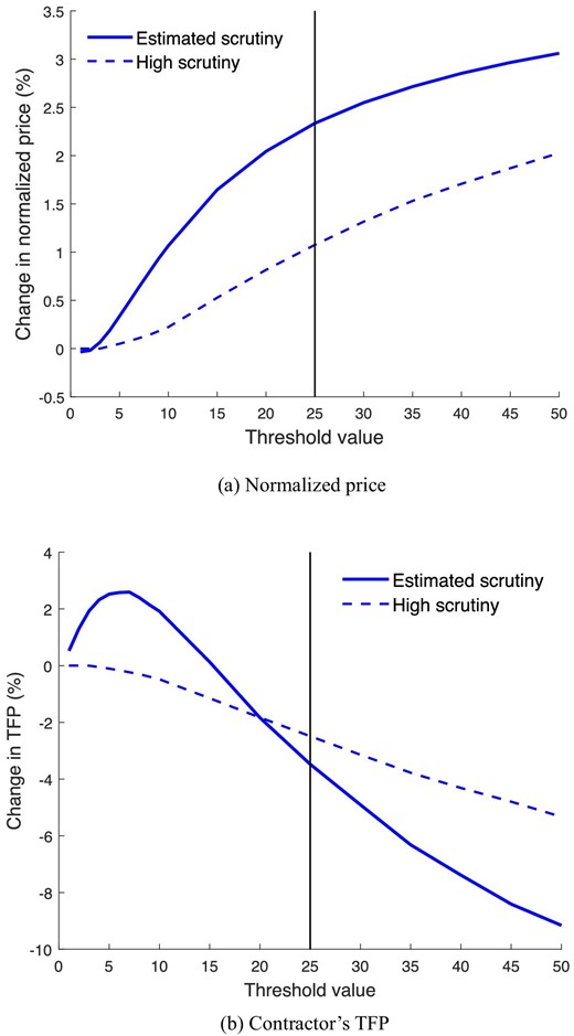
Effects of thresholds on value weighted average outcomes.
The solid lines in Figure 7 show results under the estimated level of scrutiny—using the estimated demand for discretion. Figure 7(a) plots the percentage change in average normalized price relative to the zero threshold benchmark as a function of the threshold. The main message of Figure 7(a) is that the smaller the threshold, the lower the average price. This is because sorting is based on tender characteristics that are not very relevant for price determination, so the direct (positive) effect dominates. The figure shows that the policy reform of 2011 increased the price of public procurement by 2.3%. The picture is more complicated for the average contractor TFP depicted by Figure 7(b). On the one hand, the direct effect is negative since discretion results in the selection of less productive contractors. On the other hand, the tender characteristics driving the sorting into discretion are negatively associated with productivity, introducing a second positive effect. The balance of these two counteracting effects is based on the size of the threshold. The introduction of a very small threshold increases the value weighted average productivity of contractors. As the the threshold exceeds 15 million forints, the direct effect prevails and the overall effect turns negative. I find that the policy reform of 2011 decreased productivity by 3.5% and the effect would increase to 9.2% with a 50-million threshold. The optimal threshold in terms of productivity would be around 7 million forints; relative to this optimal policy, the 25-million threshold results in a 6% drop in productivity.
The dashed lines in Figure 7 depict the relationships between value thresholds and procurement outcomes under the high level of scrutiny.33 High scrutiny prevents agencies to artificially fit contract values below the threshold. In line with intuition, increasing scrutiny has a clear negative effect on prices at all thresholds. However, the impact of scrutiny on contractor productivity depends on the size of the threshold. As we have seen earlier, for small thresholds, the positive indirect effect is strong, making the bunching of contracts beneficial and therefore the scrutiny harmful to average productivity. The impact of scrutiny flips sign (and becomes positive) for large thresholds where the negative direct effect of introducing a threshold dominates the positive indirect effect. This result highlights an important interaction between different dimensions of the optimal procurement design.
The second set of simulations allows us to compute the contribution of contract value distortions to the total impact of the policy reform. Bunching of tenders below the threshold is responsible for 54% of the reform’s total effect on prices and 28% of its total effect on productivity.
7. Conclusion
This paper shows that buyer’s discretion substantially affects procurement outcomes. To reach this conclusion, I address the endogeneity of the procedure choice by exploiting the introduction of a value threshold to estimate a structural model of procurement decisions. I find that discretion increases prices and gives rise to the selection of less productive and politically connected contractors. Using a fully parametric version of the model, I document that in product categories with more connected firms agencies are willing to sacrifice more contract value to increase their discretion. These results are in line with political favoritism being one of the underlying mechanisms. I provide suggestive evidence to rule out alternative mechanisms; I show that agencies do not use discretion to benefit domestic, local, or incumbent firms but to favor short-lived companies.
The method developed in this paper provides an alternative to the RD bounds proposed by Gerard, Rokkanen, and Rothe (2020) in dealing with a manipulated running variable. If time variation in the size of the cutoff is available, my method provides a feasible way to estimate the treatment effect, even if the manipulation is so large that it makes the RD bounds uninformative. Applications may extend beyond public procurement and can include measuring the effects of unemployment benefits and other welfare programs or investigating the consequences of anti-trust policies such as merger reviews (Wollmann 2019).
I conclude by discussing the broader policy context of my results. Bureaucratic discretion exists as part of a complex policy environment and it certainly shapes outcomes in interaction with other institutional details, such as legal liability, monitoring, and conflict of interest rules. This idea is formalized in Bosio et al. (2020), which argues that discretion only pays off in countries with high government effectiveness. Hungary is characterized by lax auditing practices and limited liability of procuring officials. Although Hungary has conflict of interest rules preventing public officials to become firm representatives in contractor firms, these rules are often bypassed by using front companies or companies owned by politicians’ family members.34 As a result, by focusing on a country with relatively weak institutions, it is not surprising that this paper finds more detrimental consequences of discretion than other empirical investigations (Coviello et al. 2022). Indeed, bureaucratic discretion may be more desirable if complemented with rigorous auditing practices and stricter ex-post liability rules. Nevertheless, most middle income and developing countries have similarly weak institutions as Hungary, so my results underscore the benefits of limiting bureaucratic discretion in a weakly institutionalized environment.
Acknowledgments
I thank David Card, Decio Coviello, Ernesto Dal Bo, Stefano DellaVigna, Mitch Downey, Frederico Finan, Vitalijs Jascisens, Supreet Kaur, Kei Kawai, Patrick Kline, Gerard Roland, Giancarlo Spagnolo, David Stromberg, Adam Szeidl, Steven Tadelis, Silvia Vannutelli, Jason Wittenberg, Guo Xu, and conference and seminar participants for many helpful comments and suggestions. I thank the European Research Council under the European Union’s Seventh Framework Program (FP7/2007-2013) grant agreement number 283484 and the European Research Council (ERC) under the European Union’s Horizon 2020 research and innovation programme grant agreement number 724501 for funding.
Notes
The editor in charge of this paper was Imran Rasul.
Footnotes
This finding is in line with Tas (2022), which documents bunching using data from all European Union (EU) countries.
Under the two assumptions mentioned above, it may provide a structural alternative to the RD bounds developed by Gerard, Rokkanen, and Rothe (2020) in the case of large manipulations in the running variable.
In the 2011–2013 period, the invitational procedure took the form of a direct negotiation without an announcement. From November 2013, procurers could also choose a simplified auction where only invited firms can bid.
To maintain a minimum level of competition, public agencies using invitational procedures have to invite at least three firms.
The invitational procedure is combined with quality assessment substantially—about 25 percentage points—less often than open auctions, suggesting that discretion may function as a substitute for scoring auctions.
The matching is based on partial or full match of names in the procurement and balance sheet data.
The partial correlation between a successful match and high discretion when controlling for a flexible function of the contract value in the post-reform period is 0.0006 (p-value = 0.921).
In about 7% of all tenders, the winning bid was less than a third of the anticipated contract value. Checking a few announcements manually suggested that in these cases the winning bid records the unit price, while the anticipated value approximates total costs resulting in extremely low normalized prices. To correct these mistakes, I excluded tenders with normalized prices below -1 (which means that the winning bid is less than a third of the anticipated value).
I use a panel of firms with at least three employees in the 2006–2018 period to estimate the production function for two digit industries. I measure capital with the total tangible assets and use material cost as a proxy to control for unobservables.
During the 2009–2015 period, 405 of the 500 top procurement winners have won a non-construction tender.
Although, there might be important unobserved quality dimensions not captured by the productivity of the selected firm, such as the match quality between the agency and the contractor or incentives for contract execution.
Since price manipulation is done by the agency, I assume that when it plans its expenses it can correct for the intentional bias in the reported contract value.
In all baseline specifications, I approximate |$f(V_i)$| with a third-order polynomial of |$\log (V_i)$| but in a robustness check, I also estimate it nonparametrically.
One can test the independence of |$\nu _i$| and |$u_i$| directly by plotting the distribution of |$u_i$| in the pre-reform period conditional on different contract values. Following this strategy, Online Appendix Figure A7 plots the residuals of the price and productivity equations conditional on three quantiles of the value distribution separately.
A smaller |$h(\nu _i)$| means that the utility gain from discretion is larger for a given |$d_i$|.
Where |$\sigma ^2_d = \sigma ^2_{\epsilon }+\varphi ^2\sigma ^2_u - 2 [ \rho _{\epsilon ,u}+\varphi \sigma ^2_u ]$|, |$\rho _{u,d} = \frac{ \rho _{\epsilon ,u}+\varphi \sigma ^2_u}{\sigma _d \sigma _u}$|.
Derivation is in the Online Appendix.
Derivation of the likelihood function is in the Online Appendix.
Table A6 in the Online Appendix suggests that this reduction in the number of bidders is not the primary channel of the negative price and productivity effects.
The significant negative coefficient of the control function in column (3) also indicates the sorting of low-productivity tenders.
There was no other policy change at the same time, so I assume that all other changes happen continuously.
I execute this by including an indicator for all bins of anticipated contract value.
I classify a product category connected intensive if at least 5% of the total value in the pre-reform period was awarded to connected firms.
In each column, I control for a cubic function of log-value, procuring agency, and year fixed effects.
Product categories where at least 80% of total contract value in the pre-reform period were allocated to domestic companies. These product categories gave 18% of all contracts in the 2009–2015 period.
I look at a 3 year window after the contract decision because my balance sheet data runs until 2018, which does not allow a longer window for all contractors in my procurement data.
I measure connected share by the share of the total value awarded to connected (top 500) companies during the pre-reform period in the product category of the contract.
Similarly to connected firms, I measure the domestic share by the share of total contract value awarded to domestic firms during the pre-reform period in the product category of the contract.
The contractor’s log-TFP is not observed for all contracts.
This sorting of tenders allows the model to capture the closing gap in the productivity of open auction winners between the pre- and post-reform periods above the threshold plotted in Online Appendix Figure A8(b).
I formalize high scrutiny by setting |$h(\nu _i) = \infty \cdot 1(\nu _i>T)$| in equation (14).
Scandals involving the son-in-law of Prime Minister Viktor Orban is a prominent example of this phenomenon (Norman and Komuves 2018).
