


Abstract
In response to a change in interest rates, younger firms not paying dividends adjust both their capital expenditure and borrowing significantly more than older firms paying dividends. The reason is that the debt of younger non-dividend payers is far more sensitive to fluctuations in collateral values, which are significantly affected by monetary policy. The results are robust to a wide range of possible confounding factors. Other channels, including movements in interest payments, product demand, profitability, and mark-ups, are also significant but seem unlikely to explain the heterogeneity in the response of capital expenditure. Our findings suggest that these types of financial frictions play an important role in the transmission of monetary policy.
1. Introduction
Investment plays an important role in the business cycle. It accounts for a significant share of domestic output, is one of its most volatile components and plays a prominent role in many macroeconomic theories. From a policy perspective, a commonly held view is that investment is a key channel of monetary transmission. This is reflected in a sizable literature in empirical macroeconomics, which, using aggregate time series data, finds that movements in interest rates have a large and persistent impact on business investment.
There remains, however, a surprising degree of uncertainty about the specific channels through which monetary policy affects investment. On the one hand, neoclassical models emphasize the direct effects of interest rate changes on the user cost of capital and firms’ expected returns. In contrast, the financial accelerator literature appeals to the more indirect effects that work through the revaluation of assets and net worth, which subsequently affects firms’ ability to borrow for investment (see, for instance, Kiyotaki and Moore 1997; Bernanke, Gertler, and Gilchrist 1999). In this second strand of the literature, monetary policy can gain extra traction over investment by influencing the borrowing constraints facing firms. There has been much debate about the empirical relevance of these financial accelerator effects, especially in the aftermath of the 2008 financial crisis, but evidence remains elusive.1
We use firm-level panel data for the United States to examine the relevance of a financial accelerator in the transmission of monetary policy. The first challenge we face is that financial constraints are not directly observable. In this paper, we focus on firm age and whether a firm pays dividends as likely correlates of exposure to a financial accelerator mechanism at the firm-level. The motivation for this comes from a number of observations. First, firms that (i) pay dividends and (ii) use debt counter-cyclically are unlikely to be constrained. A main reason is that, in the face of adverse shocks, dividend payers can reduce payouts. But, non-dividend payers are more likely to require external finance and face a larger wedge between internal and external funding costs. Indeed, in a number of models with financial frictions, credit constrained firms do not pay dividends, particularly in transition to their optimal scale.2 Second, and relatedly, firms are more likely to face financial constraints earlier in their life cycle, when they typically lack stable cash flows and have yet to develop a long credit history, a point emphasized in the firm dynamics literature (e.g. Haltiwanger, Jarmin, and Miranda 2013 and Davis and Haltiwanger 2019). Moreover, younger firms secure a far larger share of their borrowing using assets rather than earnings, whereas the opposite is true for older companies (Lian and Ma 2021). As a result, these firms are more likely to be exposed to the traditional financial accelerator type mechanisms.3
We establish four main findings. First, both the investment and borrowing of younger firms not paying dividends exhibit a large and significant decline in response to a tightening of monetary policy. Second, collateral values fall significantly for all firms when interest rates increase. Third, the borrowing of the younger non-dividend payers is far more sensitive to fluctuations in collateral values than other firms. Fourth, relative to younger non-dividend payers, the investment adjustments of older companies are much smaller (both in terms of economic and statistical significance) and the change in borrowing is insignificant. The heterogeneity we document is robust to a wide range of sensitivity analyses, including controlling for other individual characteristics such as size, leverage, and liquidity, exploiting within-firm variation over the life-cycle and using alternative strategies to identify monetary policy innovations.
What do these findings tell us about the transmission mechanism? Our preferred interpretation is that younger non-dividend payers are more likely to be constrained by the value of their assets. In particular, we show that our results are consistent with a mechanism where falling collateral values leads to tighter borrowing constraints, which amplifies the effects of monetary policy on the investment of constrained firms. In the Online Appendix, we corroborate this intuition using a stylized financial accelerator model featuring a collateral constraint. Firms differ in their optimal scale and the borrowing constraint may become less binding as they approach the optimal size. We interpret distance to optimal scale as firm age. When the indirect effects via asset prices are large, the investment and borrowing of constrained firms are more sensitive to changes in the interest rate. In Section 5, we show that other channels, including direct movements in interest payments, product demand, profitability, firms’ costs, and mark-ups are associated with more homogeneous effects and, thus, cannot easily account for the estimated heterogeneity in the investment and borrowing responses we find across groups.
Turning to the aggregate implications, we document that, despite accounting for less than one tenth of aggregate investment, younger firms paying no dividends account for around two thirds of the average effect on the investment rate (which normalizes capital expenditure by the firm’s capital stock) and for about one quarter of the response of aggregate investment to monetary policy. Furthermore, differences in the behavior across groups is informative about the importance of the indirect effects associated with financial accelerator type frictions. Our results suggest that these indirect effects—working through changes in collateral values and corporate debt—can account for around one third of the dynamic effects of monetary policy on aggregate investment. As a result, these types of channels remain an important part of the monetary transmission mechanism.
Looking at financial heterogeneity has a long tradition in empirical macroeconomics and finance. Yet, a more recent literature has shown that traditional characteristics—such as size, liquidity, and leverage—are unlikely to measure financial conditions. For instance, Crouzet and Mehrotra (2020) find that the investment of small firms is more sensitive to the business cycle than for large firms but their debt is not, which is hard to square with size capturing access to credit. Indeed, while many firms are born small and wish to grow over time, others have no ambition to expand (see Hurst and Pugsley 2011). According to Bates, Kahle, and Stulz (2009), firms tend to accumulate cash holdings to hedge against future borrowing constraints, implying that businesses with high liquidity may not be unconstrained. Finally, Lian and Ma (2021) note that many companies tend to finance M&A activities with debt rather than equity, thereby becoming significantly more levered despite having good access to financial markets.
More generally, many of the individual characteristics that have been previously used to measure heterogeneity in financial conditions tend to mix-up firms at different points in their life cycle. This chimes with the conclusion in Dinlersoz et al. (2018), who argue that one cannot fully understand the link between firm characteristics and financial frictions without conditioning on age. Our results based on age/dividend status are robust to controlling for other individual characteristics (such as size, leverage, and liquidity), whereas the heterogeneity estimated along these latter dimensions tends to disappear after controlling for age/dividend status. Furthermore, our strategy has a significant econometric advantage. Grouping strategies based on size, liquidity, and leverage suffer from several endogeneity and selection issues discussed in Section 2. In contrast, age is fully pre-determined and dividends payouts occur independently from monetary policy changes: We find that when firms begin paying dividends, they rarely stop.
Based on the age/dividend grouping strategy, our empirical analysis looks at heterogeneity in the dynamic responses of groups of firms to interest rate changes across a wide range of firm-level variables. We focus on U.S. public firms from S&P Compustat, which has excellent coverage and a long time dimension. In the working paper version of our work (Cloyne et al. 2018), we also show a companion set of results for the United Kingdom. To study the dynamic effects of monetary policy, we need a time series of identified exogenous innovations to policy interest rates. This ensures that our exogenous variation is not driven by other macro factors and also limits any potential reverse causality issues. We exploit the high frequency surprises in interest rate futures contracts within a 30 minute window around policy announcements, following Gürkaynak, Sack, and Swanson (2005), Gertler and Karadi (2015), and Nakamura and Steinsson (2018a). We then employ a local projection instrumental variable (LP-IV) panel approach to estimate the dynamic effects of monetary policy. To explore heterogeneity across firms, we interact policy rates with bins of the age/size/leverage/liquidity distribution. This strategy allows us to conduct a semi-parametric multivariate analysis by flexibly defining our bins using the outer product of various firm characteristics. For instance, we can compare the behavior of younger and smaller firms with the relative behavior of younger and larger companies to isolate the contribution of size conditional on age. A similar strategy allows us to examine the contribution of age conditional on size, for example.
Related Literature.
Our findings connect to four strands of empirical work. A important recent line of research reveals that the use of asset-based, cash flow-based, interest coverage-based covenants, and credit lines is pervasive among U.S. public firms (Drechsel 2023; Greenwald 2019; Greenwald, Krainer, and Paul 2021; Lian and Ma 2021) and both the incidence and the nature of the constraint could matter. In particular, Lian and Ma (2021) report that asset-based borrowing is the primary form of corporate debt among small, young, and low-profit firms, whereas large, old, and high-margin companies rely mainly on cash flow-based lending. Our strategy can therefore shed particular light the importance of the asset-based financial accelerator type mechanism: young non-dividend paying firms are indeed the group whose (i) investment and borrowing exhibit the largest and most significant response to interest rate changes and (ii) borrowing is most correlated with changes in collateral values.
A well-established empirical literature, exemplified by the studies of Davis, Haltiwanger, and Schuh (1996), Haltiwanger, Jarmin, and Miranda (2013), Dinlersoz et al. (2018), Pugsley, Sedláček, and Sterk (2021), and Sedláček (2020) has shown that firm age is a key determinant of employment and leverage dynamics over the business cycle. Relative to these influential works, we focus on identified monetary policy changes and investigate the dynamic responses of investment, borrowing, debt composition, and collateral values at the firm-level across demographic groups.
The importance of collateral constraints for firms is the focus of Chaney, Sraer, and Thesmar (2012), Liu, Wang, and Zha (2013), Catherine et al. (2022), and Bahaj, Foulis, and Pinter (2020). Relative to these contributions, we look at heterogeneity in the response of borrowing by age/dividends and associate this with heterogeneity in the investment responses to identified monetary policy shocks. The behavior of constrained and unconstrained firms is particularly important for assessing the indirect effects of monetary policy via financial frictions.
A large empirical literature on investment has proposed various measures of financial conditions, including cash flows (Fazzari, Hubbard, and Petersen 1988, Oliner and Rudebusch 1992), size (Gertler and Gilchrist 1994), paying dividends (Fazzari, Hubbard, and Petersen 1988), bank debt (Ippolito, Ozdagli, and Perez-Orive 2018), leverage (Ottonello and Winberry 2020 and Lakdawala and Moreland 2021), and liquidity (Jeenas 2019).4 We find that sorting firms along the joint distribution of age and dividend payouts (i) generates the largest and most significant comovement between investment and borrowing, and (ii) is robust to further conditioning on size, leverage, and liquidity, while the reverse is not true.
On the theoretical side, our evidence provides support for the notion that financial frictions amplify the effects of macroeconomic shocks in the spirit of Kiyotaki and Moore (1997) and Bernanke, Gertler, and Gilchrist (1999). Unlike these contributions where constrained firms are more levered, however, we show that being younger and paying no dividends is a far stronger predictor of a significant comovement between investment and debt, consistent with those firms being more dependent on external finance to fund their projects. Albuquerque and Hopenhayn (2004), Khan and Thomas (2013), and Begenau and Salomao (2019) feature models where firms may grow out of their borrowing constraints as they approach their optimal scale but, along this path, dividends are zero.
Structure of the Paper.
In Section 2, we present the data, discuss our age/dividend grouping strategy and document how balance sheet variables and other characteristics vary over a firm’s life-cycle. In Section 3, we discuss our empirical framework and identification strategy before presenting the average effect in our firm-level panel data. The heterogeneous response of capital expenditure following a change in monetary policy is the focus of Section 4. We show that our grouping strategy based on age and dividends predicts a larger capital expenditure response than size, leverage, and liquidity, but also that our finding is robust to conditioning on these more traditional proxies. In Section 5, we investigate the channels that may explain the heterogeneous effects on investment and show that the response of borrowing and collateral values to changes in the interest rate is the most likely candidate. We also conduct a simple calculation of the likely contribution of these asset-based financial frictions to the aggregate investment response to monetary policy shocks. In Section 6, we show that our results are robust to exploiting variation within firms and across collateral shares, to alternative strategies for identifying the time series of monetary policy shocks and to potential sub-sample instability across sectors and over time. The Online Appendix contains further robustness checks and a simple financial accelerator model whose predictions are consistent with our empirical findings.
2. Data
In this section, we briefly describe the firm-level data and discuss the construction of the main variables of interest for our empirical analysis. In particular, we introduce our measure of firm age and argue that, together with dividend payment status, are informative of the financial and life-cycle position of a firm. Finally, we present a number of descriptive statistics suggesting that younger firms may face worse access to financial markets. A more detailed description of the sources, definitions, and sample selection can be found in Online Appendix A.
2.1. Sources and Variables Definition
Detailed, high quality balance sheet and income statement data for publicly listed companies are available quarterly from Compustat. Consistent information for a sufficiently large number of firms and variables only begins around 1986, when our sample starts. The sample ends in 2016, when the data were collected for this project. Turning to our main variables of interest, the investment rate is defined as capital expenditures in period |$t$| relative to the level of physical capital, as measured by net plant, property, and equipment at the beginning of the period.5 In addition to being a widely-used measure (see e.g. Chaney, Sraer, and Thesmar 2012), it allows us to compare the investment decision of firms with different levels of capital.
The main balance sheet variables of interest are cash-flows, which we proxy with EBITDA (earnings before interest, tax, depreciation, and allowances) as is common in the literature, total and long term debt, collateral values (market value of corporate real estate), sales, and interest expenditure. In our analysis, we will also use information on dividends paid, firm size (book value of total assets), leverage (total debt divided by the book value of total assets), liquidity (short term cash and investments divided by the book value of total assets), growth (growth in total assets), and Tobin’s (average) Q (the ratio of market value of assets to book value).6 More detailed information on data sources, variable definitions, and sample selection are provided in Online Appendix A.
As a first step toward a macro analysis with micro data, we are interested in understanding how much of the aggregate investment dynamics is captured by publicly traded firms.7 To do so, we aggregate the investment reported by each firm for a given period of time into a measure of investment at calendar frequency. Online Appendix A Figure A.1 compares the growth rate of this series from Compustat with the growth rate of aggregate investment from the U.S. Bureau of Economic Analysis, which includes investment by both public and private firms.
While publicly listed companies account for about 60% of the level of investment in the U.S. economy, the dynamics of the capital expenditure series aggregated from micro data are very similar to the dynamics of the official investment data from national accounts. More specifically, the correlation of the growth rate of capital expenditure from the micro data and the growth rate of official aggregate business investment is around 0.8. Understanding the dynamic behavior of publicly listed companies can therefore provide important insights about the transmission of economic shocks to the aggregate economy.
Finally, to the extent that private firms face similar or even tighter financial conditions than public firms, our findings may be interpreted as a lower bound for the relevance of financial frictions for the transmission of monetary policy to business investment.
2.2. Grouping Firms by Age and Dividend Payouts
The first step in our research design is to identify which type of firm is most likely to face some form of financial constraint. In a broad class of theoretical macro finance models, it can be shown that financially constrained firms do not engage in dividend payouts, see, for example, Khan and Thomas (2013), Albuquerque and Hopenhayn (2004) and Begenau and Salomao (2019). In these set-ups, a firm that is currently financially constrained (or may become so in the near future) might eventually grow and become unconstrained. Until that happens, however, the firm finds it optimal to use any available resources for growth and it does not pay dividends along this path. Contributions in the financial accelerator tradition such as Crouzet and Mehrotra (2020), Ottonello and Winberry (2020), and Jeenas (2019) also feature constrained firms that do not pay dividends.
As for age, a long-standing tradition in the empirical literature on consumption using household-level data (see e.g. Attanasio and Browning 1995; Wong 2021) and on employment using firm-level data (see, for instance, Haltiwanger, Jarmin, and Miranda 2013; Davis and Haltiwanger 2019) has provided evidence consistent with the notion that being young is correlated with the unobserved characteristics driving access to external finance. Younger firms typically have less experience in credit markets, have a shorter credit history (and therefore lower rating), and tend to have lower earnings and fewer assets to pledge than their older counterparts, implying they might have less funds available for investment.
Taking these two sets of results together, younger firms paying no dividends may face a more limited access to credit markets than older dividend payers. Our favourite interpretation is that, we are capturing a firm at the point in their life cycle when they are most likely to face financial constraints: when they are younger and not paying dividends. Younger firms are likely to be further away from their optimal scale, are seeking to grow but may lack the credit history to reduce their costs of external finance.8 Moreover, these are the firms that may be most subject to traditional financial accelerator type mechanisms as their borrowing is more likely to be secured against assets (Lian and Ma 2021). Our empirical approach therefore sheds light on the importance this mechanism.
Other measures of heterogeneity in financial conditions suffer from several potential challenges and are likely to mix-up firms at different points in their life cycle. This is consistent with Dinlersoz et al. (2018), who show that, to understand the relationship between firm characteristics and financial frictions, it is important to consider the age of the firm. As documented by Hurst and Pugsley (2011), most small businesses have little ambition to grow and while young businesses tend not to be large, many old companies choose to remain small and are therefore likely to be unconstrained. The absolute size measure of financial conditions traditionally used in earlier applied work would classify these old firms as constrained simply because they are small in absolute sense. In contrast, younger firms paying no dividends are more likely to be faraway from their optimal size and, as such, face a higher probability that financial constraints might constrain their growth. In this sense, firm age is capturing a firm’s relative size.
Similar concerns apply to using liquidity or leverage as measures of financial conditions at the firm-level. A large body of empirical work has shown that firms hold more cash to hedge against the possibility of a financial constraint binding in the future (Bates, Kahle, and Stulz 2009): Firms with large cash holding have a strong precautionary motive that makes them fundamentally different from businesses with low liquidity. As noted by Lian and Ma (2021) and Begenau and Salomao (2019), many older and larger firms have a higher leverage ratio because they have good access to capital markets and tend to finance large projects with debt rather than equity. On the other hand, a lower debt to asset ratio may be the very result of a younger company with insufficient internal funds being denied further external funds.9
Another advantage of our age/dividend grouping strategy is rank invariance. A company’s starting date is fully pre-determined and age cannot vary as a result of changes in monetary policy or the business cycle. Furthermore, we find that the decision to pay dividends is independent from movements in interest rates and when a company starts paying dividends it rarely stops.10 In contrast, size, leverage, and liquidity endogenously respond to shocks or vary over the cycle, which affect the ranking of firms in the distribution of these variables. Accordingly, it is hard to interpret any (ex-post) heterogeneity as being driven exclusively (or even partially) by ex-ante differences in these specific firm characteristics.11
Many papers examining firm-level investment have focused on U.S. Compustat data where the native age variable is sparsely populated. Interestingly, however, the year of incorporation is available for U.S. publicly listed companies from WorldScope. We therefore merge these datasets to provide a consistent measure of the incorporation date. To help address some missing observations as well as the issue of mergers and acquisitions, we also make use of the first date the firm appears in the Center for Research in Security Prices data. More details on the construction of the age variable are provided in Online Appendix A. While it is possible to use information on the founding years of firms, these are only available for a limited number of companies.12 Reassuringly, however, the descriptive statistics reported in the next section using our age proxy are very similar to the correlations reported by Dinlersoz et al. (2018) measuring age as years since foundation among publicly listed companies using the Census Bureau’s Longitudinal Business Database from 2005 to 2012.
2.3. Descriptive Statistics
In the previous section, we have discussed the conceptual reasons for why capturing a firm at a particular point in its life cycle might be a better proxy for financial constraints, particularly if we are interested in the role of financial accelerator type mechanisms. In this section, we want to establish the main empirical characteristics of younger and older companies to illustrate this point further. While the evidence in this section is of course only suggestive, in the rest of the paper, we will show that younger non-dividend payers is the group of firms displaying the strongest positive comovement between investment and debt following a monetary policy shock. This comovement is consistent with the predictions of a class of financial frictions models emphasizing the role of collateral constraints.
A simple but formal way of assessing the association between our measure of corporate age and other firm characteristics is to regress each of the characteristics of interest against a polynomial in age together with a measure of firm size (for all regressions except the one for size) and the interaction between sector and year fixed effects, which are designed to clean for common trends at the sectoral level. This specification is similar to the regressions used by Dinlersoz et al. (2018) and facilitates a comparison with their results based on administrative data.13 Our dependent variables in the first column of Figure 1 are (i) size, in the first row (ii) asset growth, in the second row, (iii) Tobin’s Q, in the third row, and (iv) EBITDA (as a share of past assets), in the fourth row. In the second column, we report the relationship between age and selected firms’ financial variables such as: (v) leverage, in the first row, (vi) the probability of having engaged in dividend payouts or buy back shares in the previous year or ever having issued bonds, in the second row, (vii) credit performance—measured by credit ratings among bond issuers—in the third row, and (viii) liquidity, in the last row.14
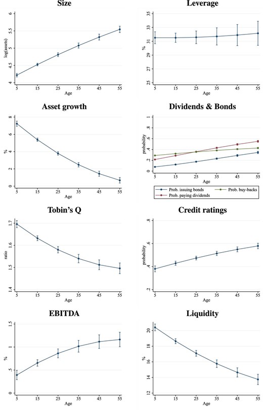
Descriptive statistics by age. Each panel reports the predicted values for each variable by age. Each panel uses a regression of the variable of interest on age and age squared conditional on sector-time fixed effects and firms’ controls as detailed in Section 2. 90% standard error bands. Standard errors are clustered by firm and time. Size is measured by the log of total assets. Asset growth is the growth rate of total assets. Tobin’s Q is the ratio of the market value of total assets to the book value. EBITDA is earnings before interest tax and depreciation, measured as sales net of costs divided by total assets. Leverage is total debt relative to total assets. Dividends and bonds are based the probability of paying cash dividends, buying back stock or having a issued a bond. Credit rating captures the probability that a firm of a given age has an investment grade (higher than BBB) rating on its (short or long term) debt. Liquidity means total short term cash and investments relative to total assets.
The top row in the first column of Figure 1 reveals that firm size is monotonically increasing with age, both in the full sample of firms that record assets and the smaller sample reporting also the number of employees. In line with Davis, Haltiwanger, and Schuh (1996), the second row confirms a sharp negative association between growth and years since incorporation; The third row shows that older companies tend to have lower Tobin’s Q values, while the fourth row reveals that younger firms have smaller or even negative operating profits early in their life.
The second column of Figure 1 examines the financial variables. Less experienced companies appear (weakly) less levered (first row),15 are less likely to pay dividends or issue bonds (second row), have worse credit scores (third row) and tend to hold a higher share of liquid assets (last row).16 The results on the relationship between leverage and age is consistent with the results based on years since foundation for publicly listed companies in Dinlersoz et al. (2018). The statistical association of age with the probability of paying dividends and Tobin’s Q is consistent with the predictions of the model in Cooley and Quadrini (2001).
In summary, our descriptive analysis reveals that, on average, younger firms are smaller, have lower cash-flows/earnings, worse credit scores, and a lower probability of paying dividends or issuing bonds. On average, they also grow faster, have a higher Tobin’s Q, hold more cash, and have lower leverage, although, interestingly, it is hard to see much difference in leverage across the age distribution. Finally, a comparison with the results in Dinlersoz et al. (2018) suggests that years since incorporation (used in this paper) and years since foundation (used in their paper) correlate similarly with other firm characteristics.
3. Empirical Framework
In this section, we describe our identification and empirical strategy. In particular, we first discuss the way we construct the time series of monetary policy shocks. We then move to our main empirical specifications. In the final part of this section, we present the estimates of the average effect of interest rate changes on investment in the micro-data at the firm-level and show this compares well with standard results from the macro literature using data from national statistics.
3.1. Identification
Identifying the dynamic causal effects of monetary policy on investment requires tackling the potential reverse causality: interest rates respond to the economy and also affect it. This is a standard problem in the empirical macro literature (see Nakamura and Steinsson 2018b), but it poses a further challenge in the context of our panel micro data analysis. We need our estimated effects to be driven by exogenous changes in monetary policy and by not some other macro factors causing movements in interest rates. Furthermore, some of the firm groups that we consider account for sizable movements in aggregate variables. This implies that some monetary policy responses to aggregate conditions may be, in fact, correlated with specific conditions in a particular group. As in the macro literature, we need some exogenous variation in policy rates.
Our identification strategy is based on the proxy-VAR/external instrument approach of Mertens and Ravn (2013) and Stock and Watson (2018), applied to monetary policy by Gertler and Karadi (2015). The idea is to isolate interest rate surprises using the movements in financial markets data within a short window around central bank policy announcements. Building on Gürkaynak, Sack, and Swanson (2005), Gertler and Karadi (2015) measure financial market surprises from Fed Funds Futures, using a 30 minutes interval around the FOMC policy announcements. The plausible identifying assumption is that nothing else occurs within this time window, which could drive both private sector behavior and monetary policy decisions. The technical innovation in Gertler and Karadi (2015) is to use these high frequency surprises as proxies for the true structural monetary policy shocks in a Vector Autoregression.17
Data on Fed Funds Futures are available since 1991, while the firm-level data span the period 1986–2016. One advantage of the Mertens and Ravn (2013) and Stock and Watson (2018) proxy-VAR used by Gertler and Karadi (2015) is that even if the identification of the contemporaneous causal relationships is based on the sample for which the proxy/instrument is available, the VAR can be estimated over a longer sample. This allows us to identify a sequence of monetary policy shocks for a longer period than the instrument is available for. We use the implied monetary policy shocks from the Gertler and Karadi (2015) VAR as our measure of monetary policy shocks in the micro data, obtaining a time series of monetary policy innovations for the full sample: 1986–2016.18 The approach only requires the high frequency surprises to be contemporaneously exogenous and the VAR will purge any remaining predictability. Furthermore, by directly following Gertler and Karadi (2015), our micro results will be more directly comparable to the macro literature (as we show in Online Appendix C). For all these reasons, this method is preferable to using the financial surprises directly in the panel estimation.19
We estimate a reduced-form VAR for the period 1986–2016, keeping as close as possible to the specification in Gertler and Karadi (2015). The VAR includes a measure of interest rates, log industrial production, the log of the consumer prices index, and two proxies for financial conditions.20 The time series of the monetary policy shocks is shown in Online Appendix B, together with the time series of the high-frequency monetary policy surprises. These policy shocks are then used in our firm panel regressions: As these are exogenous disturbances, there is no need to include further macro controls. We have also verified that our estimates do not suffer from a weak instrument problem.
To estimate the dynamic causal effects from the micro data, we use a panel LP-IV set up, following Jordà, Schularick, and Taylor (2020). This is very flexible and allows us to estimate impulse response functions on firm-level panel data using the identified monetary shocks as instruments for interest rate changes. There are two advantages of using the monetary policy shocks as an instrument rather than as a regressor directly. First, the scale of the shock (from the proxy-VAR) is indeterminate but as shown by Stock and Watson (2018) (page 11), the LP-IV estimation automatically imposes the unit effect normalization, implying that the size of the shock can then be interpreted in terms of the units of the endogenous variable, namely the interest rate. Second, as discussed by Wooldridge (2002, p. 117), generated instruments do not suffer from the inference problem associated with generated regressors highlighted by Pagan (1984).21
3.2. Baseline Specification
In order to capture the heterogeneous effects of monetary policy, in our benchmark empirical specification, we estimate impulse response functions using an instrumental variable (IV) variation of the LP approach, LP-IV:
Time is denoted by |$t$| and the data are quarterly. |$i$| denotes a firm. The dependent variable |$X$| will be the variable of interest: the investment rate in Section 4 and borrowing, collateral value, sales, and cash flows in Section 5.22|$\Delta R_t$| is change in the one year interest rate used in Gertler and Karadi (2015), instrumented using our extracted series of monetary policy shocks.23|$Z_{t-1}$| is a set of firm characteristics and the indicator function takes a value of 1 if the firm characteristic falls in a particular “bin” of the distribution, which we will refer to as the firm’s group. Importantly, |$Z$| can be multidimensional and we can have separate slopes for finer groups, for example, young/small/low leverage, old/large/high leverage, etc. In essence, this is a semi-parametric way of estimating the heterogeneous effects of monetary policy by different (and possibly multivariate) firm characteristics. We are not, therefore, imposing the restrictive assumption of linearity in these interactions. This is something that turns out to be important and also distinguishes us from virtually all earlier contributions working on investment heterogeneity at the firm-level. We also do not include other time or sector-time fixed effects as we want to interpret these coefficients as group specific impulse response functions, including any general equilibrium effects. This allows us to estimate conditional impulse response function as flexibly as possible.24 But we do add firm fixed effects, which not only absorb any sector fixed effect but also allows us to exploit also within-firm variation. Furthermore, we include quarterly dummies to control for seasonal factors.25 The end of quarter interest rate (interacted with the dummies) will be instrumented by the monetary policy shock (also interacted with the dummies). Standard errors are clustered by firm and time using the approach in Driscoll and Kraay (1998) for dealing with possible serial correlation in the forecast errors |$\epsilon _{i,t+h}$|, which is potentially a feature of LPs. The number of lags is set to 12. Finally, we estimate IRFs over a forecast horizon of 5 years, so we restrict the sample to firms that we observe for at least 5 years (20 quarters).
3.3. The Average Effect
Before presenting the results for different groups, it is useful to estimate the average response of the investment rate to a change in monetary policy in our firm-level panel data. This provides a benchmark against which we can evaluate the contribution of each group of firms. It also allows us to see whether the dynamic response of investment in the micro data resembles the impulse response functions we typically see in the time series macro literature.
To estimate the average effect, we drop the group dummies from equation (1) and replace the group-specific coefficients on the interest rate with a single parameter |$\beta _{h}$|. |$\beta _{h}$| therefore captures the average effect of interest rates on the investment rate at horizon |$h$|.
Figure 2 reports the impulse response function up to 20 quarters. The investment rate declines significantly following a 25 bp rise in the interest rate. The effect becomes significant towards the end of the first year and the peak effect is reached between the second and third year after the shock, at a value around |$-0.5$|pp. The shape of the dynamic response is broadly consistent with the impulse response functions obtained using aggregate data. These are shown in Online Appendix C. The dynamics of the average investment rate (estimated from the micro data) therefore lines up well with the macro response of business investment from national statistics. Online Appendix C also shows that our empirical approach generates results that reflect the macroeconomic effects found in Gertler and Karadi (2015). We are therefore starting from a standard set of benchmark macro results.
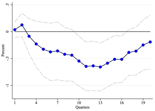
Average response of investment to an increase in interest rates. This figure shows the impulse response function (IRF) for the investment rate following a 25 bp increase in the one year interest rate. The IRFs are estimated using the LP-IV approach described in the text. The regression does not allows for heterogeneity across groups and the IRF is therefore the average effect across all firms in the sample and facilitates comparison with macroeconomic IRFs using time series data. Dotted lines are 90% standard error bands. Standard errors are computed using the Driscoll–Kraay method, clustering by firm and time, which is robust to very general forms of cross-sectional and temporal dependence.
Having established a benchmark against which to study the heterogeneous responses of capital expenditure across different groups of firms, our goal in the next section is to “disaggregate” this average effect and examine which groups drive the response and why.
4. The Response of Investment across Firms
In the previous section, we have shown that younger firms tend to be smaller, earn less, have lower a credit rating and (weakly) lower leverage, pay no dividends, issue no bonds, and accumulate more cash. While we have argued that these descriptive statistics are consistent with worse access to credit markets, our goal is to evaluate this claim by looking at the joint behavior of investment and the firm balance sheet in response to a change in monetary policy. The hypothesis is that in the presence of financial accelerator type frictions, which link net worth or asset values to a firm’s borrowing capacity, constrained firms should adjust both their investment and debt more than unconstrained firms. This logic is sketched out in the simple model in Online Appendix M.
In this section, we show that younger non-dividend payers indeed change their capital expenditure far more than any other group. We also show that while more traditional proxies of financial frictions—such as size, liquidity, and leverage—also generate some heterogeneity in the dynamic effects of monetary policy, the marginal predictive power of each of these traditional measures disappears once we conditions on our age/dividends proxy. The reverse, however, is not true: The heterogeneity by age and dividends status is robust to controlling for other proxies. Finally, we quantify the contribution of younger firms paying no dividends to the average investment response to monetary policy and find that this is significant. In the next section, we examine the channels of monetary transmission in more detail by showing the responses of debt and other variables.
4.1. Results Based on Age and Dividends
In this section, we explore the role of financial heterogeneity using our grouping strategy. More specifically, we allow the effects of monetary policy to vary across the age and the dividend status distribution. We split the sample into four groups depending on whether a firm is younger (less than 15 years since incorporation) and whether it paid dividends before the monetary policy shock. While there is no conceptual reason to prefer one specific age cutoff over another, the results are not sensitive to the precise threshold.26 The first (second) row of Figure 3 shows the impulse response functions for younger (older) firms. The first (second) column in each block refers to non-dividend (dividend) payers. Comparing the two rows reveals the marginal contribution of age, controlling for dividend status. Comparing the columns reveals the marginal contribution of paying dividends, controlling for age.
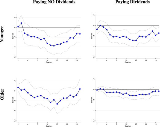
Response of investment by age and dividend status. This figure shows the impulse response functions for the investment rate following a 25 bp increase in the one year interest rate. The interest rate is interacted with binary indicators based on age and dividend status. Younger refers to <15 years since incorporation and older refers to >15 years since incorporation. No dividends means the firm did not pay cash dividends in the previous year. The IRFs are estimated using the LP-IV approach described in the text. Dotted lines are 90% standard error bands. Standard errors are computed using the Driscoll–Kraay method, clustering by firm and time, which is robust to very general forms of cross-sectional and temporal dependence.
There are three main results that emerge from Figure 3. First, the initial effect over the first few quarters is small and insignificant for all groups, but the peak for younger non-dividend payers is more than one third larger than for younger firms paying dividends.27 Second, among non-dividend payers, younger firms (top-left corner) have the largest and most significant response, with the peak effect around 1% in absolute value. Third, the adjustment of capital expenditure to a monetary policy shock for older dividend payers (bottom-right corner) is much smaller, being around one fourth on average of the response of younger firms paying no dividends.28 To assess formally the statistical difference between groups, in Figure 4, we re-run our baseline regressions adding the interest rate as a separate regressor and making older dividend payers the base category (given that this is the set of firms most likely to be unconstrained). While this strategy has the disadvantage of losing track of the average effect of monetary policy, it has the advantage of allowing us to formalize a test of whether the estimated impulse response for each group at each horizon is statistically different from the estimated impulse response of the base group, which is old-dividend payers. The figure shows that the investment response of younger non-dividend payers is significantly larger than for older dividend payers at almost all horizons. In contrast, there seems to be no statistical difference between the two groups of old companies. Finally, the capital expenditure adjustment of young dividend payers is also significantly larger than the adjustment of old dividend payers, although the relative effect is smaller (in absolute magnitude) than for younger non-dividend payers.29
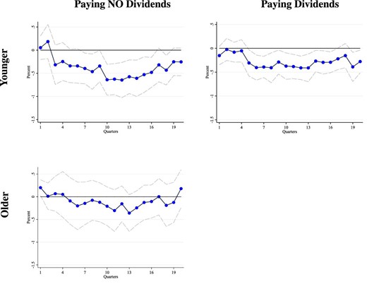
Response of investment by age and dividends relative to older firms paying dividends. This figure shows the impulse response functions for the investment rate following a 25 bp increase in the one year interest rate. The interest rate is interacted with binary indicators based on age and dividend status. Younger refers to <15 years since incorporation and older refers to >15 years since incorporation. No dividends means the firm did not pay cash dividends in the previous year. Relative to the results in Figure 3, this specification includes the interest rate as a regressor on its own. The IRFs are relative to older dividend-paying firms. The IRFs are estimated using the LP-IV approach described in the text. Dotted lines are 90% standard error bands. Standard errors are computed using the Driscoll–Kraay method, clustering by firm and time, which is robust to very general forms of cross-sectional and temporal dependence.
In Online Appendix D, we report results based on splitting the sample only along the age dimension (Figure D.1) or only according to whether a firm paid dividend or not (Figure D.2). Consistent with the estimates in Figure 3, we find in Figure D.1 that younger firms respond far more than either middle-aged firms (with incorporation date between fifteen and fifty years before the shock) or older firms (with more than fifty years since incorporation). Similarly, in Figure D.2, we document that non-dividend payers respond far more than dividend payers. Interestingly, however, the response of younger non-dividend payers in Figure 3 is larger than either younger firms in Figure D.1 or non-dividend payers in Figure D.2. Indeed, this is the reason why we conclude that the combination of age and dividends status is a stronger predictor of a larger investment response than each of these dimensions in isolation. We see dividend status and age as complementary indicators, where the goal is to capture a firm precisely at the point in its life cycle where particular asset-based financial constraints are most acute.
4.2. Conditioning on Other Firm-Level Characteristics
The evidence above reveals that being younger and paying no dividends is a strong predictor of a larger response of investment to monetary policy changes. In Section 2, we have shown that younger firms tend to be smaller, hold more cash, and are weakly less levered relative to older firms. In Online Appendix E, we consider each of these dimensions in isolation and find that the adjustment of smaller firms is stronger than for larger ones, that the investment response of less levered companies is larger than for more levered ones and that businesses with higher liquidity change capital expenditure more than firms holding less cash. This is not surprising given that all these proxies, including age, are correlated with each other. In Section 2, we have argued on a conceptual basis that age and dividend paying status combined are likely to be better proxies for certain types of financial constraints than these more traditional characteristics. In this section, we want to assess the relative merits of the age-dividend split on statistical grounds.30
Unlike traditional panel regression analyses in which the identification exploits exogenous variation in the cross section, our identification strategy is based on exogenous changes (in monetary policy) that vary over time but are common across firms, while allowing for heterogeneous slopes along a variety of dimensions. Accordingly, the notion of “controlling for other characteristics” requires a different approach than simply adding further regressors to our baseline empirical specification. To examine the marginal contribution of age conditional on other characteristics, we interact the four age/dividends groups with quartiles of the size/leverage/liquidity distribution. This is essentially controlling for the third variable in a semi-parametric manner, a strategy that we refer to as triple-cutting the data or triple sorting.
By looking at the differences between the response of smaller-younger-paying no dividends firms and the estimated effects on smaller-older-paying dividends companies, for instance, one can infer the marginal contribution of age and paying dividends status for a given (smaller) size. Similarly, by comparing smaller-younger-paying no dividends firms to larger-younger-paying no dividends companies, we will be able to assess the marginal contribution of size for a given (younger) age and (paying no) dividends status.
As triple sorting is very demanding on the data, we maximize the number of observations per sub-group by using only two categories for age and two categories for the other characteristics. We maintain the same two age groups from above (based on fifteen years since incorporation). Dividend status is already binary. In terms of the third dimension of interest, we use the most responsive quartile versus the rest of the distribution. To stick with the size example, this means comparing the bottom quartile of size (smaller firms) with the rest of the distribution. This outer product generates eight bins. The results by size, leverage, and liquidity in isolation are reported in Online Appendix E. The full set of impulse response functions for all 8 groups generated by the triple-interaction are reported in Online Appendix F. For sake of exposition, Figure 5 focuses on younger firms paying no dividends versus older firms paying dividends, conditional on the most responsive group according to the third dimension.
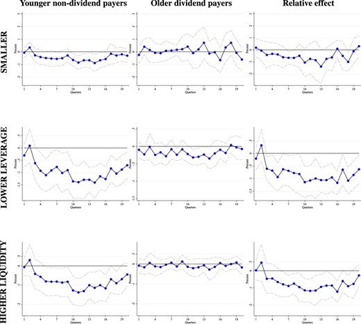
Controlling for other firm characteristics. This figure shows the IRFs for the investment rate following a 25 bp increase in the one year interest rate. We run separate regressions for each row. In each row, the interest rate is interacted with three sets of group dummies based on a firm’s age, dividend status and their position in either the size, leverage or liquidity distribution. Younger means less than 15 years since incorporation. Size refers to total assets in the previous year. Leverage is total debt relative to assets in the previous year. Liquidity is cash relative to total assets in the previous year. For size, leverage and liquidity we display the results using the most responsive quartile when the data are cut using these variables alone (see Online Appendix E). Smaller and lower leverage refers to the bottom quartile of each distribution. Higher liquidity refers to the top quartile of the liquidity distribution. The relative effect column refers to separate specifications where the IRFs are estimated relative to older firms paying dividends. The IRFs are estimated using the LP-IV approach described in the text. Dotted lines are 90% standard error bands. Standard errors are computed using the Driscoll–Kraay method, clustering by firm and time, which is robust to very general forms of cross-sectional and temporal dependence.
In the first row of Figure 5, we show that among the smaller companies, only the younger non-dividend payers in the first column adjust their capital expenditure significantly after a monetary policy shock. In contrast, the investment response of small older dividend payers in the second column is not statistically significant. The third column shows the relative effect. As in Figure 4, this column formalizes the test of a difference between the two groups. The third column of the first row therefore shows that small younger-non dividend payers have a much larger response and this is statistically significant at various points in the impulse response horizon. The rest of Figure 5 paints a very similar picture for leverage and liquidity. Among the firms with lower leverage (second row) or with more liquidity (third row), younger non-dividend payers is always the group that adjusts investment the most, as measured by the point estimates. Furthermore, the relative effect in the third column reveals that the response of younger non-dividend payers is significantly larger than for old paying dividend firms.31
Overall, the results in Figure 5 show that younger non-dividend payers drive the larger responses of smaller firms, of less levered companies and of more liquid businesses reported in Online Appendix E (where we split the sample according to each of these characteristics in isolation). Finally, the predictive power of size, leverage, and liquidity is not robust to “controlling for” age. The results are shown in Online Appendix Figure F.1: Once we condition on being young and paying no dividends, we find little differences among firms based on size, leverage, and liquidity. This means that our age based measure is a more direct proxy for the underlying characteristics that predict a larger sensitivity to monetary policy. Once we condition on age, the power of other common proxies is greatly muted. The full set of results for all groups are also shown in Online Appendix F.
In summary, age and dividend status are strong predictors of significant heterogeneity in the response of capital expenditure to changes in monetary policy. This is true over and above any possible heterogeneity by size, leverage, and liquidity. In contrast, the heterogeneity along these traditional (and arguably endogenous) proxies for financial constraints appears weaker than the heterogeneity based on age and dividend status and, more importantly, becomes marginally insignificant once we condition on being young and paying no dividends.
4.3. Contribution to the Average Effect and the Aggregate Investment Response
The evidence in Figure 3 suggests that younger non-dividend payers are likely to drive the average effect on the investment rate in Figure 2. To verify this more formally, we now compute the share of the average response accounted for by this group. We first calculate the (discounted) cumulative percent response in the investment rate for younger non-dividend payers and multiply this by their average investment share (relative to the total investment in the sample). Dividing this object by the sum of the same statistics across all groups provides an estimate of the contribution of younger no-dividend firms to the average response of the investment rate. As might be expected from Figures 2 and 3, this is a sizable number: younger non-dividend payers account for around 2/3 of the average movement in the investment rate in the sample.
A related question is about the contribution of younger non-dividend payers to the response of aggregate investment (rather than of the average investment rate, which normalizes a firm’s capital expenditure by its capital stock). To answer this, we make use of the approximation in continuous time below. A detailed derivation can be found in Online Appendix G. The contribution of each group to the effect of monetary policy on aggregate investment (|$I_{t}$|) can be expressed as a function of the response of the investment rate |$i_{j,t}$| for firm group |$j$| and the size of that group. Specifically, the overall percentage change in aggregate investment, |$\dot{I}_{t}/I_{t}$| can be decomposed as follows:
where |$\omega _{j,t}^{k} \equiv k_{j,t}/K_{t}$| (average capital for group |$j$| relative to the aggregate capital stock) and |$\omega _{j,t}^{I}\equiv I_{j,t}/I_{t}$| (average investment for group |$j$| relative to aggregate investment). |$\dot{i}^{\mathit {net}}_{j,t} \equiv \partial (i_{j,t}-\delta )/\partial r_{t}$| is the estimated group response of the investment rate to monetary policy in Figure 3 and |$\omega _{j,t}^{k}$|, |$\omega _{j,t}^{I}$|, and |$I_{t}/K_{t}$| are computed from Compustat. Finally, |$t$| refers to the entire IRF horizon and we focus on the average response over 20 quarters.
Applying this decomposition reveals that young non-dividend payers account for around |$21\%$| of the response of aggregate investment to monetary policy. This is remarkable given that the capital stock of this group is only |$6\%$| and their share of aggregate investment is only |$8\%$|.32 In short, while younger no dividend firms account for a rather small share of the investment level, their contribution to the aggregate investment changes due to monetary policy is considerably larger.33
5. The Channels of Monetary Transmission
In the previous section, we have shown that younger firms paying no dividends exhibit the largest and most significant adjustment in capital expenditure following a change in interest rates. While traditional proxies of financially constrained firms—such as size, leverage and liquidity—also generate heterogeneity in capital expenditure, the differences across groups are smaller and disappear after conditioning on age and dividend status.
In this section, we examine why younger non-dividend payers respond more. Specifically, to assess the hypothesis that these firms are more exposed to a financial accelerator mechanism, we look at a number of variables from firms’ balance sheet and income statements, paying special attention to the response of collateral values and debt. In particular, we show that the heterogeneity in the response of capital expenditure is mirrored by the response of debt. In contrast, the change in earnings, sales, and interest payments are more homogeneous across groups. This sizable comovement of debt and investment supports the idea that our proxy is indeed capturing a particular form of financial constraints, which are more acute for younger non-dividend payers. This latter group is populated by firms that are also more profitable, growing faster, and/or exhibit higher return volatility. These factors, however, do not explain the results in the previous section: We will show that, although more profitable and higher volatility companies tend to respond more to monetary policy, the effect is driven by the sub-group of younger non-dividend payers.
5.1. Borrowing, Collateral Values, and Financial Frictions
A number of theories emphasize the role of firm balance sheets in amplifying the effects of changes in monetary policy. Higher interest rates lower asset prices and push down equity values. This may lead to a rise in the external finance premium and generate a further decline in investment (as in Bernanke, Gertler, and Gilchrist 1999). Higher interest rates can also trigger a fall in collateral values and lead to a tightening of borrowing constraints whenever a significant portion of debt is secured against collateral (as in Kiyotaki and Moore 1997). The key is that these indirect effects are sufficiently large to trigger amplification though a sizable reduction in borrowing and investment for constrained firms. The simple model in Online Appendix M corroborates this interpretation.34 Since these asset-based channels have important implications for firms’ financing decisions and their balance sheets, in this section we look at how firms’ borrowing decisions and collateral values respond to changes in monetary policy.
A natural place to start is with the response of borrowing. Financial accelerator theories predict that the borrowing of constrained firms should respond more whenever (i) their debt is secured against collateral, and (ii) collateral values are highly sensitive to changes in monetary policy. In the top row of Figure 6, we report the response real debt growth, which we take as a measure of debt issuance. In the bottom row, we show the response of firms’ collateral at market value (bottom row). This is constructed using changes in the book value of real estate collateral and movements in real estate prices at the state-level, in the spirit of Lian and Ma (2021) and Chaney, Sraer, and Thesmar (2012).35 The left column shows the findings for younger non-dividend payers, the middle column refers to older firms paying dividends. As before, to formally test for a statistically significant difference between the groups, the third column estimates the relative response of younger no-dividend firms, using older dividend payers as reference group in a specification that also includes the interest rate as a separate regressor.
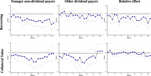
Response of firm finance: borrowing and collateral. This figure shows the IRFs for the investment rate following a 25 bp increase in the one year interest rate. We run separate regressions per each row. The first row shows the response of total real debt growth (annualized). The second row shows the response of real collateral value growth (market value). The market value of collateral is constructed using the change in the book value of corporate real estate assets and using state house price variation as discussed in the data appendix (Online Appendix A). Young refers to less than 15 years since incorporation. The relative effect column refers to separate specifications where the IRFs are estimated relative to older firms paying dividends. The IRFs are estimated using the LP-IV approach described in the text. Dotted lines are 90% standard error bands. Standard errors are computed using the Driscoll–Kraay method, clustering by firm and time, which is robust to very general forms of cross-sectional and temporal dependence.
Two main findings emerge from Figure 6. First, the decline in borrowing after a monetary policy tightening is large and significant at most horizons for younger non-dividend payers.36 In contrast, the change in borrowing for older firms paying dividends is economically modest, being on average less than one third of the effects for younger non-dividend payers and statistically insignificant at almost all horizons. Second, collateral values (in the bottom row) decline for all firms after an increase in interest rates. This is consistent with the notion that credit conditions tighten for financially constrained firms whose borrowing is secured against the value of their collateral.37
To examine further whether the debt of younger non-dividend payers is more sensitive to fluctuations in collateral values, we follow a recent and growing literature on debt covenants, which has documented significant heterogeneity in the types of borrowing contracts across groups of firms. Lian and Ma (2021), for instance, report that asset-based borrowing is more prevalent among younger firms, who lack stable cash flows and typically have not an extensive credit history. On the other hand, earning-based borrowing is predominant among old and large companies. To explore this heterogeneity, we project changes in long-term debt on collateral values and earnings, measured by EBITDA as in Lian and Ma (2021) and Drechsel (2023). We also control for firm fixed effects, as well as other characteristics including size, leverage, liquidity, and Tobin’s Q. Our focus is on heterogeneity in the correlations of borrowing with collateral values and with earnings, by age/dividend status. Standard errors are clustered by firm and time. Table 1 reports the results. The first four rows display the sum of the coefficients on collateral (real estate at market value scaled by lagged total assets), while the bottom four rows show the coefficients on earnings scaled by lagged total assets. The four columns analyze the sensitivity of our estimates across several specifications where we vary the fixed effects included in the regression.
The correlation of borrowing with collateral values and earnings.
| (1) | (2) | (3) | (4) | ||
|---|---|---|---|---|---|
| Baseline | No group FEs | Sector FEs | Region FEs | ||
| (1) | (2) | (3) | (4) | ||
| Collateral | Young no dividends | 0.106*** | 0.106*** | 0.099*** | 0.106*** |
| (0.024) | (0.024) | (0.023) | (0.025) | ||
| Young paying dividends | 0.071* | 0.088** | 0.074* | 0.075* | |
| (0.033) | (0.031) | (0.032) | (0.032) | ||
| Old no dividends | 0.034 | 0.026 | 0.031 | 0.038 | |
| (0.022) | (0.022) | (0.020) | (0.022) | ||
| Old paying dividends | 0.058** | 0.061*** | 0.059*** | 0.059** | |
| (0.017) | (0.017) | (0.016) | (0.017) | ||
| Earnings | Young no dividends | 0.022 | 0.022 | 0.020 | 0.020 |
| (0.013) | (0.013) | (0.013) | (0.013) | ||
| Young paying dividends | 0.070* | 0.070* | 0.067* | 0.069* | |
| (0.030) | (0.031) | (0.030) | (0.030) | ||
| Old no dividends | 0.019 | 0.020 | 0.015 | 0.014 | |
| (0.019) | (0.019) | (0.019) | (0.020) | ||
| Old paying dividends | 0.137*** | 0.137*** | 0.125*** | 0.114*** | |
| (0.028) | (0.028) | (0.026) | (0.028) | ||
| Time varying firm controls | |$\times$| | |$\times$| | |$\times$| | |$\times$| | |
| Firm FE | |$\times$| | |$\times$| | |$\times$| | |$\times$| | |
| Group FE | |$\times$| | |$\times$| | |$\times$| | ||
| Sector |$\times$| Time FE | |$\times$| | ||||
| Region |$\times$| Time FE | |$\times$| | ||||
| (1) | (2) | (3) | (4) | ||
|---|---|---|---|---|---|
| Baseline | No group FEs | Sector FEs | Region FEs | ||
| (1) | (2) | (3) | (4) | ||
| Collateral | Young no dividends | 0.106*** | 0.106*** | 0.099*** | 0.106*** |
| (0.024) | (0.024) | (0.023) | (0.025) | ||
| Young paying dividends | 0.071* | 0.088** | 0.074* | 0.075* | |
| (0.033) | (0.031) | (0.032) | (0.032) | ||
| Old no dividends | 0.034 | 0.026 | 0.031 | 0.038 | |
| (0.022) | (0.022) | (0.020) | (0.022) | ||
| Old paying dividends | 0.058** | 0.061*** | 0.059*** | 0.059** | |
| (0.017) | (0.017) | (0.016) | (0.017) | ||
| Earnings | Young no dividends | 0.022 | 0.022 | 0.020 | 0.020 |
| (0.013) | (0.013) | (0.013) | (0.013) | ||
| Young paying dividends | 0.070* | 0.070* | 0.067* | 0.069* | |
| (0.030) | (0.031) | (0.030) | (0.030) | ||
| Old no dividends | 0.019 | 0.020 | 0.015 | 0.014 | |
| (0.019) | (0.019) | (0.019) | (0.020) | ||
| Old paying dividends | 0.137*** | 0.137*** | 0.125*** | 0.114*** | |
| (0.028) | (0.028) | (0.026) | (0.028) | ||
| Time varying firm controls | |$\times$| | |$\times$| | |$\times$| | |$\times$| | |
| Firm FE | |$\times$| | |$\times$| | |$\times$| | |$\times$| | |
| Group FE | |$\times$| | |$\times$| | |$\times$| | ||
| Sector |$\times$| Time FE | |$\times$| | ||||
| Region |$\times$| Time FE | |$\times$| | ||||
Notes: Standard errors are in parentheses. Collateral|$_t$| is the market value of real estate (calculated using the method outlined in the text and the Online appendix) in period |$t$| relative to total assets at the beginning of the year. Earnings refers to EBITDA in period |$t$| relative to total assets at the beginning of the year. The table shows the sum of the coefficients for years |$t$| and |$t-1$| for both collateral and earnings. Firm and time-two-digit-sector fixed effects are included. Additional firm-level controls are total debt, cash holdings, and cash flows from operations all measured relative to total assets, and Tobin’s Q. Standard errors are clustered by firm and time. Standard errors in parentheses |$^{*} p<0.05$|, |$^{**} p<0.01$|, |$^{***} p<0.001.$|
The estimates in Table 1 offer two main insights. First, the borrowing of younger non-dividend payers is significantly correlated only with firm collateral.38 The coefficient on earnings is much smaller and statistically indistinguishable from zero. Second, older-dividend payers exhibit a sizable and very significant coefficient on earnings, which is much larger than their coefficient on collateral. Interestingly, young dividend payers display occasionally significant estimates on both collateral and earnings, which are roughly of equal magnitude, which connects to the discussion Section 4.3 about heterogeneity in this group of firms. As in Figure 6, these findings reveal that the borrowing of younger non-dividend payers is far more correlated with collateral values than for older companies or for firms paying dividends. The results in this section are in line with the evidence on debt covenants presented by Lian and Ma (2021), who show that—among U.S. traded companies—only the borrowing of younger firms is predominantly secured against assets, whereas the majority of older firms’ debt is secured against earnings. Lian and Ma’s finding points to the prevalence of asset-based borrowing constraints among younger non-dividend payers, consistent with the large responses and comovement between investment and debt for this group that we have documented above.
Our inference, that the response of younger-non dividend payers reflects tightening borrowing constraints, chimes with two additional pieces of evidence. First, using data on corporate bond yields, Anderson and Cesa-Bianchi (2018) show that the corporate spread increases significantly only for firms with a lower credit rating (younger firms in our sample) following a monetary policy contraction. Second, the aggregate evidence from national statistics in Online Appendix C reveals that, on average, corporate spreads and the policy rate are positively correlated after a monetary policy shock. The positive correlation between interest rates and corporate spreads is also consistent with the evidence in Gertler and Karadi (2015) and Caldara and Herbst (2019). The first finding is consistent with younger firms facing more severe financial frictions; the second result is consistent with financial frictions amplifying the effects of monetary policy.
5.2. The Responses of Cash Flows
In the previous section, we discussed a prominent example of an amplification channel: monetary policy affects firm investment via collateral values and tighter borrowing conditions. In this section, we look at three cash-flow variables that could reflect alternative channels. First, some younger non-dividend payers may have a larger share of shorter maturity debt and/or more variable rate debt. Accordingly, direct movements in interest payments might account for the heterogeneity in the capital expenditure responses reported in Section 4. Furthermore, younger firms paying no-dividends might face a product demand or a cost schedule with a higher cyclical sensitivity. If so, the response of gross sales and earnings (which are essentially sales net of costs) will be informative about whether this is driving the heterogeneous effects of monetary policy on investment. These potential explanations are explored in Figure 7, where the rows report the response of interest payments, sales, and earnings, respectively, for younger firms not paying dividends (left column) and older companies paying dividends (middle column). The relative effect between these two groups is reported in the third column for formal hypothesis testing purposes.
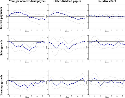
Response of firm finance: sales, earnings, and interest payments. This figure shows the IRFs for the investment rate following a 25 bp increase in the one year interest rate. We run separate regressions per each row. The first row shows the response of (log) interest payments. The second row shows the response of real sales growth (year on year). The third row shows the response of real earnings growth (measured using the real growth rate of EBITDA). The relative effect column refers to separate specifications where the IRFs are estimated relative to older firms paying dividends. Young means less than 15 years since incorporation. The IRFs are estimated using the LP-IV approach described in the text. Dotted lines are 90% standard error bands. Standard errors are computed using the Driscoll–Kraay method, clustering by firm and time, which is robust to very general forms of cross-sectional and temporal dependence.
At face value, the response of interest expenditure is hard to interpret because this is a function of both interest rates and debt decisions. However, the time profile of the impulse responses in the first row of Figure 7 is very revealing. Within the first year of the shock, interest payments increase significantly. As we have seen in Figures 3 and 6, however, neither investment nor debt respond significantly within the first year, suggesting that the movement in interest expenditure is more likely to reflect the increase in the interest rate. During the second year, the adjustment of interest payments become insignificant and after the second year it turns negative. This is consistent with the significant decline in borrowing during the first year after the shock in Figure 6 but is inconsistent with interest payments being a main driver of the significant investment responses at two and three years in Figure 3. Furthermore, there is little heterogeneity in the responses of interest payments across groups, which is formally verified in the third column of Figure 7.
Younger non-dividend paying firms may also respond more to monetary policy because the demand for their product may be more sensitive to changes in interest rates. This interpretation can be assessed from the second row of Figure 7, which reports the results for the growth of sales. These charts show that the response of sales growth over the first two years after the shock is far more homogeneous than the response of investment, with the relative difference recorded in the third column being statistically insignificant. For example, the average effect in the first six quarters is around 0.2% for both younger non-dividends payers and older dividend payers. Interestingly, some heterogeneity emerges only during the third year (after the investment responses in Figure 3 have peaked), with the highest point estimate for younger non-dividend payers around |$-0.8$| and for older dividend payers at about |$-0.5$|. We conclude that the time profile of the impulse responses of sales is inconsistent with the hypothesis that heterogeneity in product demand is a main driver of the heterogeneity in investment after a change in interest rates.
Another relevant measure of firms’ cash flows are earnings (measured by EBITDA), which—unlike gross sales—could change heterogeneously, also if costs were differentially affected by monetary policy across groups. Alternatively, following an interest rate increase, a fall in earnings could further accelerate the decline in capital expenditure if a significant fraction of firm debt is earnings-based. While we have already shown in the previous section that the debt of younger non-dividend payers is secured mostly against assets, a decline in cash flows could also trigger a shortage of internal funds, which may result in a further contraction of investment for firms struggling to attract external funds. This earning-based amplification hypothesis is explored in the third row of Figure 7. The responses of earnings are relatively homogeneous across the age/dividends groups and are not particularly sizable, especially in comparison to the response of borrowing and investment. The peak effects in the third row are around 1%, which is considerably smaller than the movements in borrowing and collateral values recorded in Figure 6. Furthermore, in dollars terms, debt is typically larger than earnings, which on average is true at all ages, as shown in Figure 1. This implies that—in dollars—the decline in borrowing for young non-dividend payers is much larger than the fall in their cash flows/earnings. This suggests that an earnings-based borrowing constraint would be less likely to explain the movements in corporate debt and investment that we observe among younger firms paying no dividends.
Together with the evidence in Section 5.1, we interpret the relatively smaller and more uniform estimates for interest payments, sales, and earnings across groups as evidence that these channels, on their own, seem unlikely to play a quantitatively major role in accounting for the heterogeneity in the capital expenditure responses in Figure 3. That said, although an earnings-based channel may be less important than an asset-based channel for younger firms, both channels would be consistent with financial frictions amplifying the dynamic effects of monetary policy.
5.3. Profitability and Growth
Another possible interpretation of the strong response of younger no-dividend firms is that, rather than being driven by financial constraints, this might reflect the fact that younger businesses may be more profitable, growing faster and more sensitive to interest rate changes. Indeed, in Section 3 we have documented that, on average, younger firms tend to have a higher Tobin’s Q and experience faster growth rates. In Appendix Figure E.2, without controlling for age or dividend status, we show that the investment of firms in the top quartile of the yearly distribution of Tobin’s Q or Alpha (from CAPM-type of regressions) respond more to monetary policy than the other groups. It should be noted, however, that the differences are less marked than using the age/dividends grouping strategy, especially for Tobin’s Q.
To consider the role of age/dividend status controlling for profitability, in Figure 8, we split the group of more profitable firms into young non-dividend payers (left column) and old dividend payers (right column) using Tobin’s Q (top row) and Alpha (bottom row). To the extent that profitability (rather than age/dividend) is the genuine driver of the heterogeneous responses of investment in Section 4, we should observe no difference between more profitable young firms and more profitable old firms. To the extent that age/dividend (rather than profitability) is the key trait associated with a larger response, then among the more profitable businesses, younger firms should adjust their investment more than old more profitable firms. Figure 8 shows that this is indeed the case: even among more profitable companies, younger non-dividend payers respond significantly more than older dividend payers (as shown in the third column), which corroborates an independent role for age/dividend status. For completeness, in Online Appendix F and in Online Appendix Figure J.2, we show that within the group of younger firms paying no dividends, there is far less variation by Alpha and Tobin’s Q.
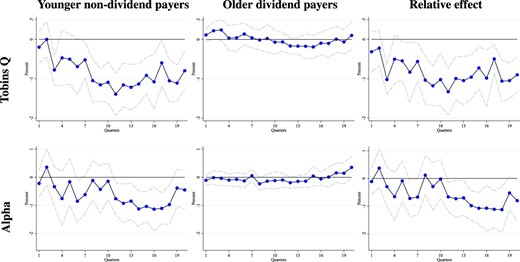
Response of investment: conditioning on Tobin’s Q and Alpha. This figure shows the IRFs for the investment rate following a 25 bp increase in the one year interest rate. We run separate regressions for each row. In each row, the interest rate is interacted with three sets of group dummies based on a firm’s age, dividend payment status and the distribution of each firm’s Tobin’s Q, and Alpha, which we estimate from a CAPM type regression. For both variables, we display the results using the top quartile of the distribution, which is most responsive group when the data are cut using these variables alone (see the Online appendix). The relative effect column refers to separate specifications where the IRFs are estimated relative to older firms paying dividends. Young refers to less than 15 years since incorporation. The IRFs are estimated using the LP-IV approach described in the text. Dotted lines are 90% standard error bands. Standard errors are computed using the Driscoll–Kraay method, clustering by firm and time, which is robust to very general forms of cross-sectional and temporal dependence.
Younger firms are not only more profitable on average but also tend to grow faster. Some profitable firms may, of course, already be at (or close to) their optimal scale. We can therefore also repeat the same exercise conditioning on firm growth. These results are also reported in Online Appendix F. Again, faster growing firms respond more to monetary policy, but within this group it is the younger non-dividend payers that drive the result.
It is important to note that while younger firms may have a higher Tobin’s Q, not all highly profitable firms are young and paying no dividends. Some profitable firms may be unconstrained, while others may still face financial frictions, especially if they are younger, not paying dividends and still growing towards their optimal scale. If profitability or growth prospects alone were the underlying driver of the heterogeneity found in Section 4, then this would survive even conditional on age/dividends. This section shows this is not the case. Even among more profitable firms, it is the younger no-dividend firms that respond considerably, as in our main results in Section 4. This reinforces the notion that our proxy is capturing firms at a particular point in their life cycle when they are most likely to face financial constraints.
5.4. Mark-Ups, Volatility, and Risk
Another confounding factor could be heterogeneity in mark-ups. Some firms, for instance, may choose a lower frequency of price adjustments and charge higher mark-ups. In Section 5.2, however, we have already documented little heterogeneity in the responses of sales and earnings across firms, which seems inconsistent with the hypothesis that mark-up heterogeneity is driving the results in Section 4. Another way of looking at this is to exploit a fact documented by Gorodinchenko and Weber (2016), that firms with stickier prices exhibit a higher volatility of stock market returns after a monetary policy shock. In Online Appendix Figure E.2, we show that firms in the top quartile of the stock market volatility distribution change their capital expenditure slightly more than their low volatility counterparts. However, Figure 9 reveals that within the high return volatility group, only younger firms paying no dividends (left column) display a large and significant response. The effect on older firms paying dividends (middle column) tends to be small and not statistically different from zero. Furthermore, the relative effect in the third column reveals that the difference across groups is statistically significant at various horizons.
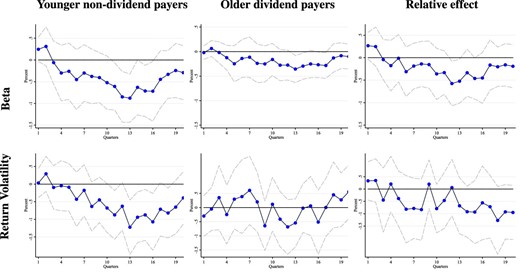
Response of investment: conditioning on beta and volatility. This figure shows the IRFs for the investment rate following a 25 bp increase in the one year interest rate. We run separate regressions for each row. In each row, the interest rate is interacted with three sets of group dummies based on the distribution of each firm’s return volatility and Beta, which we estimate from a CAPM type regression. For both variables, we display the results using the most responsive group when the data are cut using these variables alone (see the Online appendix). For volatility, we use the top quartile of the distribution, for Beta we use firms with a Beta greater than 1. The relative effect column refers to separate specifications where the IRFs are estimated relative to older firms paying dividends. Young refers to less than 15 years since incorporation. The IRFs are estimated using the LP-IV approach described in the text. Dotted lines are 90% standard error bands.
A corollary of these findings is that our main results in Section 4 are not simply driven by firms with a higher return volatility (with no role for age/dividend status). It is possible that the effects of monetary policy vary with the riskiness of the firm. This could, in principle, provide an explanation for the heterogeneity by age/dividend status. But the results in this section suggest this is unlikely to be the case. To provide further evidence on this point, we consider a further measure of risk. Online Appendix Figure E.2 shows that firms with a higher Beta (from a CAPM type of regression)—a measure of systematic risk—are more responsive to monetary policy, without conditioning on age/dividend status. In Figure 9, however, we show that this is driven by younger non-dividend payers among the higher Beta group. In contrast, older dividend payers with higher Beta exhibit only a modest change in capital expenditure. Furthermore, as shown in Online Appendix Figure J.6, there is little heterogeneity by Beta once we condition on age/dividend status.
5.5. The Contribution of Financial Frictions
In Section 4, we have shown that younger non-dividend payers account for around 2/3 of the average movement in the investment rate and about 1/4 of the aggregate investment response to monetary policy. Earlier in this section, we have argued that the larger effects on younger non-dividend paying firms is consistent with asset-based financial frictions playing a significant role for this group. In this section, we ask: What can these results tell us about the overall importance a financial accelerator in the monetary transmission mechanism?
The answer to this question necessarily depends on the view one takes about the nature of the remaining three groups. We have already noted that the investment response of both sets of older companies is significant while their debt response is not statistically different from zero. Furthermore, the estimates in Table 1 reveal that the borrowing of these two groups is the least correlated with fluctuations in collateral values. This suggest that older companies seem the least likely to face traditional financial accelerator-type frictions. We have already argued that the behavior of young non-dividend payers appear to have all the hallmarks of collateral constrained companies. In between these two extremes, we place young dividend payers: their borrowing response as well as the correlation between their borrowing and collateral values is significant, but it is not as large as for young non-dividend payers. As discussed earlier, these three groups account for around |$1/3$| of the average response of the investment rate. To the extent that all young firms paying dividends are unconstrained—which we view as a rather conservative assumption—we can obtain a lower bound on the importance of these asset-based financial constraints by comparing the contribution of younger non-dividend payers to the average effect with the contributions of the other three groups. Since younger non-dividend payers account for |$2/3$| of the average response, this implies that the indirect effects coming from these financial frictions account for around |$1/3$| of the average effect of monetary policy on the investment rate under this scenario.
Following a similar logic, we can also provide a back-of-the-envelope calculation for the contribution of asset-based financial frictions to the response of aggregate investment. As shown earlier, younger non-dividend payers account for around one quarter of the response of aggregate investment. How much of this contribution comes from non-financial accelerator channels? To answer this question, we need to come up with a counterfactual estimate of what the contribution of younger non-dividend payers would have been if they were financially unconstrained. Using the investment response of old dividend payers (which we view as the most “unconstrained” group) and the capital share of the younger non-dividend payers, we calculate this counterfactual contribution to be around |$3\%$|.39 Subtracting this from the actual |$21\%$| contribution of younger no-dividend paying firms implies that financial accelerator type frictions account for at least |$18\%$| of the aggregate investment response to monetary policy.
To move from a lower bound to a central estimate, we need to take a more realistic stand on the behavior of young companies paying dividends. The |$18\%$| lower bound is based on the extreme assumption that these companies face no financial accelerator type frictions. Consider now the other (equally unrealistic) extreme in which all young dividend payers are constrained in the same way as their non-dividend paying counterparts. Then, using the same logic outlined above, we calculate that these types of financial constraints (measured now by the response of both groups of young firms) would account for about |$42\%$| of the aggregate investment response to monetary policy. The mid-point between the upper bound of |$42\%$| and the lower bound of |$18\%$| is roughly |$1/3$| and corresponds to the case, where half of young dividend payers face significant asset-based financial frictions (or alternatively, all these companies’ exposure to financial frictions is half of the young non-dividend payers’ exposure). Accordingly, we take one third as our favourite back-of-the-envelope estimate of the contribution of these financial accelerator-type frictions to the effects of monetary policy on aggregate investment.40
External Validity.
One may reasonably ask whether our results for the U.S. are applicable more generally to other countries and samples. While we have focused on the U.S. here, in the working paper version of our work (Cloyne et al. 2018), we also repeat all the exercises presented in this paper for the U.K. We omit these here for brevity but the similarity in all the results is striking. This is interesting because the results are informative about whether the type of transmission mechanisms that we have documented may also be at work in other countries. We find this is the case. More specifically, we document that younger non-dividend payers display the largest and most significant capital expenditure response after a U.K. monetary policy shock and they are also the firms whose debt adjusts the most. Once age and dividend status is controlled for, however, other proxies for financial constraints no longer generate sizable heterogeneity. In line with the U.S. results, younger British firms paying no dividends tend to be smaller, have lower leverage, lower earnings, lower credit scores and their borrowing is significantly more asset-based than any other group of firms. Finally, we show that the response of earnings and interest rate payments is more homogeneous across groups and that the indirect effects may account for more than one third of the effects of monetary policy on investment in the U.K.
6. Sensitivity Analysis
In this section, we show that our main result—that younger non-dividend payers respond more to a monetary policy shock—is robust across a range of additional exercises and specifications. In particular, our findings are confirmed when: (i) using employment growth rather than investment as the outcome variable, (ii) we consider other alternative financial constraints indices, (iii) exploiting only within-firm variation for a group of firms that we observe over their entire life-cycle and examining potential cohort effects, (iv) considering a different cut of the data using the market value of collateral across firms, (v) using three different identification strategies to isolate exogenous movements in monetary policy, and (vi) possible sub-sample instability over time and sectoral heterogeneity.
6.1. The Response of Employment
While our analysis has focused on capital expenditure, the mechanism discussed above should also affect other firm outcomes. We therefore now look at the response of employment growth to a monetary policy shock. The reason is twofold. First, labour and physical capital are often complements. Second, investment in physical capital may not fully capture a firm’s response to monetary policy, especially in the presence of intangible assets. Looking at employment growth serves as a cross-check on the heterogeneous responses that we have documented so far. The results are reported in Figure 10.
Response of employment by age and dividend status. This figure shows the impulse response functions for employment growth following a 25 bp increase in the one year interest rate. Employment is defined as the number of employees reported (Compustat variable EMP), which is only available in the annual Compustat database. To maintain the same econometric approach as used for all other results, we therefore convert these to quarterly data using linear interpolation. The interest rate is interacted with binary indicators based on age and dividend status. Younger refers to |$<15$| years since incorporation and older refers to |$>15$| years since incorporation. No dividends means the firm did not pay cash dividends in the previous year. The IRFs are estimated using the LP-IV approach described in the text. Dotted lines are 90% standard error bands. Standard errors are computed using the Driscoll–Kraay method, clustering by firm and time, which is robust to very general forms of cross-sectional and temporal dependence.
Unfortunately employment is only available in the annual version of Compustat, which naturally reduces the observations we can use and makes our results noisier. To maintain the baseline specification in the paper, we linearly interpolate employment to a quarterly series. Despite these caveats, in line with the findings for investment, the impulse responses for employment point towards strong heterogeneity in the response across firms. Furthermore, the relative magnitudes across groups mirror the findings for investment. The effect of an interest rate change on employment is significantly large and persistent for young non-dividend payers but small and short-lived for both groups of older companies. The response of young dividend payers sits in between these two extremes.41
6.2. Grouping Firms by Traditional Proxies of Financial Constraints
In Section 4, we argued that other firm characteristics such as size, leverage, and liquidity are prone to selection and endogeneity issues. Indeed, in Online Appendix E, we have shown that grouping firms along each of these dimensions reveals much less heterogeneity than splitting the sample according to age and dividend payment status. In this section, we conduct a similar exercise to Online Appendix E, but using two other popular strategies in corporate finance to elicit financially constrained firms. The first index is due to Kaplan and Zingales (1997) and combines cashflows, long term debt, dividends, cash and short term investments, and Tobin’s Q at the firm level. The second proxy comes from Hadlock and Pierce (2010) and relies mostly on firm size and, to a lesser extent, size squared and corporate age. Both these traditional measures use estimate-based weights to determine the contribution of each component to the index. A higher values indicate a more financially constrained firm.42
In Figure 11, we report the results splitting the sample according to these more traditional measures. The top row refers to the Kaplan–Zingales index, while the bottom row represents Hadlock–Pierce’s. The left (right) column reports the impulse responses of investment to a monetary policy shock for firms with below (above) median values of the index and therefore potentially captures less (more) financially constrained companies. Two results emerge from this exercise. First, there is little heterogeneity across firms based on Kaplan–Zingales measure, consistent with the notion that other firm characteristics appear more relevant to elicit differences based on access to finance. Second, above-median firms using Hadlock–Pierce’s proxy tend to adjust their investment by about twice as much as below-median firms at the peak, although the estimates tend to be less precise than those in Figure 3 for young no-dividend payers.43
Response of investment: other financial constraints indices. This figure shows the impulse response functions for the investment ratio following a 25 bp increase in the one year interest rate, splitting firms using alternative indices for financial constraints. The interest rate is interacted with binary indicators based on whether the firm has an above or below median value of each financial constraints index. The Kaplan and Zingales (1997) index |$= -1.001909 CF + 3.139193 TLTD -- 39.36780 TDIV - 1.314759 CASH + 0.2826389 Q$|, where CF = Cashflow, TLTD = Total long term debt, TDIV total dividents, CASH = Cash and short term investments, and Q = Tobin’s Q. The Hadlock and Pierce (2010) index |$= -0.737 Size + 0.043 Size^2 - 0.040\, Age$|, where Age is the minimum of age and 37 years and size is truncated at $4.5bn (2004) book assets. The IRFs are estimated using the LP-IV approach described in the text. Dotted lines are 90% standard error bands. Standard errors are computed using the Driscoll–Kraay method, clustering by firm and time, which is robust to very general forms of cross-sectional and temporal dependence.
To explore the merits of our categorization based on firm age and dividend payment status relative to the grouping strategy proposed by Hadlock and Pierce (2010), in Figure 12, we further split the above-median firms based on the Hadlock–Pierce index into young no-dividend payers in the left column, and old dividend payers in the right column. The top row reports the investment responses and the bottom row reports the response of borrowing. These results show that the larger estimates in Figure 11 for the above-median firms according to Hadlock–Pierce’s measure is driven by young firms paying no dividends, whose responses for both investment and borrowing are large and significant. In contrast, the dynamic effects of monetary policy on the behavior of above-median old dividend payers are small, both economically and statistically.44 We conclude that, while more traditional measure such as the one in Hadlock and Pierce (2010) also captures some heterogeneity in access to finance, the differences across firms appear sharper using our grouping strategy based on both corporate age and dividend payments. As we have shown in Sections 4 and 5, the behavior of young firms is consistent with these companies being more exposed to a financial accelerator type mechanism, especially when these firms do not pay dividends.
Response of investment and borrowing for Hadlock and Pierce (2010) constrained firms. This figure shows the impulse response functions for the investment ratio and total real debt growth (annualized) following a 25 bp increase in the one year interest rate for firms with an above median value of the Hadlock and Pierce (2010) index. The interest rate is interacted with binary indicators based on age, dividend status and the financial constraints index of Hadlock and Pierce (2010). Younger means less than 15 years since incorporation. The IRFs are estimated using the LP-IV approach described in the text. Dotted lines are 90% standard error bands. Standard errors are computed using the Driscoll–Kraay method, clustering by firm and time, which is robust to very general forms of cross-sectional and temporal dependence.
6.3. Within-Firm Variation over the Life-Cycle and Cohort Effects
Our baseline result compares the investment response of younger non-dividend payers to the other groups. Since our sample includes young firms who eventually become old and young firms who died or entered over the period, one concern is that these composition effects might be blurring the distinction between groups.
To address this concern, in this section, we focus on a restricted sample of old dividend paying firms that we also observe when they were young and paying no dividends. To the extent that age and dividend status are the genuine drivers of heterogeneity, we should see results that mirror our baseline findings: these firms should respond little when old but have responded significantly more when they were young and paying no dividends.
This hypothesis is confirmed in Figure 13. The chart shows the response of older firms paying dividends (in the right column), together with the response of the same firms when they were young and not paying dividends (in the left column). The capital expenditure response of these firms when they were young and not paying dividends is large and statitically significant, looking remarkably similar to the impulse response functions in Section 4. This corroborates the view that our finding of heterogeneity is genuinely driven by age and dividend status, rather than by changes in groups composition over time.
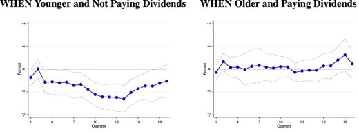
Exploiting only within-firm variation over the life-cycle. This figure shows the IRFs for the investment rate following a 25 bp increase in the one year interest rate. Only firms who eventually become old and pay dividends are kept for this exercise. We then examine the response of these firms to a monetary policy shock when they are old and when they are young. Young refers to less than 15 years since incorporation. The IRFs are estimated using the LP-IV approach described in the text. Dotted lines are 90% standard error bands. Standard errors are computed using the Driscoll–Kraay method, clustering by firm and time, which is robust to very general forms of cross-sectional and temporal dependence.
An additional concern is that our results might be influenced by cohort effects, where being young in the early part of the sample has different implications from being young later in the sample. To assess the empirical relevance of this challenge, we have also reproduced the analysis behind Figure 3 by cohort (rather than age directly) and dividend status where cohort is defined based on the incorporation date of the firm. Younger firms are those incorporated after 1977. The 1977 threshold ensures that “older” companies are at least ten years old at the start of the sample. The results in Online Figure K.1 are very similar to our baseline findings in Figure 3, revealing that the heterogeneous responses that we document in this paper are not driven by this type of cohort effects.
6.4. Low versus Highly Collateralized Firms
In Section 4, we argued that a firm facing higher costs of external finance may be less likely to pay dividends earlier in their life-cycle in an effort to retain internal funds for investment. Indeed, in the previous section, we showed that the same companies whose investment was most sensitive to monetary policy when younger and paying no dividends, became unresponsive after growing old and starting to pay dividends.
As argued by Gertler and Gilchrist (1994, pp. 312–313), informational frictions can add to the costs of external finance if companies are not well collateralized. Whenever external funds are secured against a lower level of collateral, these firms may be particularly sensitive to movements in collateral values. This is indeed the type of mechanism discussed in Section 5. But it also suggests an alternative measure of financial conditions: the share of assets that can be used as collateral. In this section, we therefore consider grouping firms based on the market value of their collateral (scaled by total assets).
There are pros and cons to this strategy. On the one hand, grouping firms by their collateral share may speak more directly to the type of financial frictions that we seek to investigate in our empirical analysis. On the other hand, there are several disadvantages. First, the market value of collateral has to be imputed (which, as discussed in Section 5, we do by using the market value of real estate at the state-level) and thus is likely to be measured with error. In contrast, age and whether a company pays dividends or not are observed with virtually no measurement error in every quarter of our sample. Second, the market value of collateral is endogenous and responds significantly to changes in interest rates. This implies that firms may move from one group to another in response to monetary policy shocks. In contrast, age cannot vary with interest rate changes and therefore is not subject to this selection issue.
Despite the drawbacks, it is still instructive to consider this further split of the data. Prima facie evidence that our age/dividend grouping strategy may be correlated with a firm’s collateral position comes from noting that, on average, younger non-dividend payers tend to have less collateral on their balance sheets. For example, the market value of real estate relative to overall (net) plant, property, and equipment is |$17\%$| and only |$5\%$| when measured as a share of total assets. On the other hand, the same ratios for older companies paying dividends is much higher, at |$46\%$| and |$13\%$|, respectively. Of course, not all young firms have a low collateral share and, conversely, not all old firms have a high share.
In Figure 14, we therefore split firms in eight bins depending on their age (below or above 15 years since incorporation), whether they pay dividends or not and whether their collateral share (market value of real estate as a share of total assets) is above or below the median of the sample distribution in each year. The rows denote age. The even (odd) columns refer to paying (no) dividends. The four panels on the left (right) represent firms with below- (above-) median collateral share within each group.
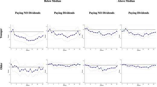
Response of investment by age, dividends paid and collateral share. This figure shows the IRFs for the investment rate following a 25 bp increase in the one year interest rate. The interest rate is interacted with binary indicators based on age, dividend status, and size. Younger refers to <15 and older refers to >15 years since incorporation. No dividends means the firm did not pay cash dividends in the previous year. Below median refers to those firms below the median market value of collateral/lagged total assets in the previous year. The IRFs are estimated using the LP-IV approach described in the text. Dotted lines are 90% standard error bands. Standard errors are computed using the Driscoll–Kraay method, clustering by firm and time, which is robust to very general forms of cross-sectional and temporal dependence.
To the extent that the share of pledgable assets drives access to external finance and thus the investment response of younger non-dividend payers, we would expect that—within this group—younger non-dividend payers with a below median collateral share would adjust their capital expenditure in response to monetary policy much more than younger non-dividend payers with an above median collateral share. On the other hand, within each of the other groups, which are unlikely to face significant collateral constraints, there should be little difference in the investment responses of low versus highly collaterized firms.
Two main results emerge from Figure 14. First, the peak response of low-collateral younger non-dividend payers (in the top left corner) is twice as large as the response of high-collateral younger non-dividend payers (in the panel on the first row of the third column). Second, whether a firm is below or above the median collateral share makes little difference to the investment responses within each of the other three age/dividend groups (in the second and fourth columns as well as in the bottom row of the first and third columns).
The findings in this section are consistent with the notion that the larger investment response of younger non-dividend payers reported in Section 4 reflects, at least partially, the heterogeneity in collateral shares exploited in this section. While we still favour the grouping strategy based on dividend payment status because of its higher coverage, absence of measurement error and independence from changes in monetary policy, we interpret the results in this section as further evidence that we are identifying the exposure of a firm to collateral-based financial frictions.
6.5. Identification of Monetary Policy Shocks
In this section, we consider a number of alternative ways of identifying exogenous variation in monetary policy. One popular method has been proposed by Romer and Romer (2004), who isolate the residuals of a Taylor-type rule by projecting changes in the target federal funds rate on the Federal Reserve Greenbook forecasts of the change in inflation, unemployment, and output growth. In the first row of Figure 15, we show the results based on Romer and Romer’s identification for the period 1986–2007.45 As in Romer and Romer (2004) we use the Romer and Romer shock directly in the baseline regression. We focus on the results for younger non-dividend payers (left column) versus older dividend payers (right column). The third column reports the relative effect. The estimates confirm, by and large, the heterogeneity in the capital expenditure responses along the age/dividend dimension.
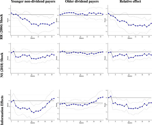
Response of investment using different shock identification schemes. This figure shows the IRFs for the investment rate following a 25 bp increase in the one year interest rate. Relative to Figure 3: (i) The first row uses the Romer and Romer (2004) shocks (extended by Wieland and Yang 2020 to 2007) in the main regression. This series only uses data to 2007 given the lack of variation in the Federal Funds Rate after 2008. (ii) The second row reconstructs the monetary policy shocks by re-estimating the Gertler and Karadi (2015) proxy-VAR using the high frequency “Policy News Shock” from Nakamura and Steinsson (2018a). (iii) The third row includes controls for the change in the central bank’s forecast for GDP, inflation and unemployment for the current quarter and two and four quarters ahead. Forecast data come from the Philadelphia Fed’s Greenbook Data Set. Results are similar including more forecasts although the standard errors become wider. The IRFs are estimated using the LP-IV approach described in the text. Dotted lines are 90% standard error bands. Standard errors are computed using the Driscoll–Kraay method, clustering by firm and time, which is robust to very general forms of cross-sectional and temporal dependence.
As a second robustness check, we use a different measure of the high frequency monetary surprise. Instead of using the high frequency surprises from Gertler and Karadi (2015) to identify our monetary policy shocks, we follow Nakamura and Steinsson (2018a) and use their Policy News Shock as the instrument. This variable is the first principal component of the change in several interest rate variables in the 30 minute window around the policy announcement. This shock may contain richer information about the policy surprise and is therefore a very useful alternative. The second row of Figure 15 reveals that our findings are robust also to using this alternative high frequency instrument.
Finally, a recent literature, pioneered by Nakamura and Steinsson (2018a), Miranda-Agrippino and Ricco (2021), and Jarociński and Karadi (2020), emphasize that high frequency movements in short-rate futures around the policy announcements may also reveal information about the central bank’s view of the economy. Romer and Romer (2000) document that Federal Reserve policy announcements contain signals about the Fed’s private information and private forecasters tend to update their forecasts as a result. High frequency surprises might therefore be a mix of a genuine monetary policy surprise and an information effect (e.g., the central bank becomes more/less optimistic about the economy than previously thought). While this does not invalidate our strategy to isolate exogenous variation in monetary policy, it may affect the interpretation of our results. In the final row of Figure 15, we therefore conduct a further robustness check. Miranda-Agrippino and Ricco (2021) suggest controlling for central bank forecasts as a way of netting-out the information effect. We reproduce our main specification augmented with the changes in the central bank forecasts for inflation, GDP and unemployment around the policy decisions. This adds a number of additional parameters to estimate, which would become very demanding if we made this the baseline specification for all the exercises in the paper. But, reassuringly, the estimates are very similar to the baseline results in Figure 3: The response of young non-dividend payers is large and significant, whereas the response of old firms paying dividends is small and statistically insignificant. We conclude that our results are not being driven by an information effect.
6.6. Sub-Sample Stability and Sectoral Effects
This section considers whether our estimates are overturned by dropping the recent financial crisis, controlling for differential time trends and effects across industrial sectors. Since these exercises either limit the number of observations or greatly increase the number of parameters to be estimated, we show these results as sensitivity analyses.
The top row of Online Appendix Figure L.1, shows the investment response of younger non-dividend payers dropping the period after 2007. While the bands are marginally wider, the responses are still large and significant for this group. In contrast, older firms paying dividends do not respond at all over this shorter sample, confirming that the heterogeneity we find in Figure 3 is not driven by the financial crisis. To some extent, this result could have been anticipated from the previous section, where we showed that a completely different shock identification scheme (Romer and Romer 2004) that ends in 2007 also produced similar estimates.
Next, we consider whether our results are sensitive to controlling for industrial sectors. We do this in two ways. First, the second row of Online Appendix Figure L.1 shows the dynamic effects of monetary policy on the capital expenditure of younger firms not paying dividends when we add sector-time fixed effects. This specification allows for different time trends by industrial sector. The third row allows the marginal effect of interest rate changes to vary by industrial sector.46 In using time fixed effects, the impulse response functions in both exercises are relative to one of the age-dividend groups. Without loss of generality, we report the results relative to the old firms paying dividends group, which is the least responsive group. We still find a relatively stronger investment adjustment for younger firms paying no-dividends. The main result in Figure 3 therefore holds over and above any possible heterogeneity across sectors.
7. Conclusions
This paper asks two main questions: (i) Do financial frictions matter for the transmission of monetary policy? (ii) How much do they contribute to the aggregate investment response? The answer to the first question is: “yes, they do”. The answer to the second question is: “around 1/3”. We reach these conclusions after a detailed firm-level analysis of the heterogeneous responses of balance sheet and income statement variables from the universe of U.S. public firms. The quest for these answers allows us to identify firm characteristics that are most likely to correlate with the presence of these types of financial frictions.
Younger firms paying no dividends tend to be smaller, have lower credit ratings, earn less, and access less credit. Most importantly, the borrowing of this group is most sensitive to fluctuations in collateral values. As interest rate increases significantly affect firms’ collateral values, younger non-dividend payers are forced to reduce borrowing and therefore cut investment. In contrast, older firms paying dividends adjust their investment by much less and the change in their borrowing is modest, statistically and economically. Other channels, including changes in interest payments, product demand, firms’ costs, and mark-ups, generate little heterogeneity across firms and thus seem unlikely to explain our findings.
A further contribution of our analysis is to show that the combination of age and dividend-payment status is a far stronger and more robust predictor of a large positive comovement between investment and borrowing than other firm characteristics such as size, leverage, and liquidity. In our favourite interpretation, we are capturing a firm at the point in their life cycle in which they are most likely to face asset-based financial frictions: when they are younger and not paying dividends. Younger firms are likely to be some distance from their optimal scale, are seeking to grow but are probably still missing the necessary historical record in credit markets to access low cost external finance. A simple collateral constraint model with heterogeneity in optimal size generates predictions on the heterogeneous effects of monetary policy on investment and borrowing across constrained and unconstrained firms that are in line with our empirical evidence by age/dividends status. Overall, our findings highlight an important role for a financial accelerator in the transmission of monetary policy to investment.
Acknowledgments
We are grateful to Adrien Auclert, Saleem Bahaj, Saki Bigio, Florin Bilbiie, Colin Cameron, Thomas Chaney, Larry Christiano, Nicolas Crouzet, Juan-Antolin Diaz, Thomas Drechsel, Martin Eichenbaum, Angus Foulis, Nicola Gennaioli, Mark Gertler, Yuriy Gorodnichenko, Oscar Jorda, Sebnem Kalemli-Ozcan, Peter Karadi, Yueran Ma, Joseba Martinez, Emi Nakamura, Elias Papaioannou, Gabor Pinter, Giorgio Primiceri, Vincenzo Quadrini, Ayşegül Şahin, Martin Schneider, Petr Sedláček, Stefanie Stantcheva, Jon Steinsson, Alan Taylor, Philip Vermeulen, Gianluca Violante, and participants at many seminars and conferences for very useful comments and suggestions. We also thank Diego Kaenzig and Ezgi Kurt for excellent research assistance. The views in this paper are those of the authors and do not necessarily reflect the views of the Bank of Spain, the Euro-system, or the Bank of England. Surico gratefully acknowledges financial support from the European Research Council (Consolidator Grant 771976). Cloyne is affiliated at NBER and CEPR. Surico is affiliated at CEPR.
Footnotes
We note that financial frictions might dampen the response of a constrained firm precisely because it is harder to access funds. Our focus is therefore on whether certain financial frictions can generate large indirect effects.
Interestingly, Gertler and Gilchrist (1994) note that “the informational frictions that add to the costs of external finance apply mainly to younger firms, firms with a high degree of idiosyncratic risk, and firms that are not well collateralized. These are, on average, smaller firms” (pp. 312–313. Emphasis added). We are grateful to Ayşegül Şahin for kindly reminding us of this quote.
Several later studies have warned that the investment sensitivity to cash flows should not be interpreted as evidence in favor of financial frictions as cash flows can be shown to be a determinant of investment in both theoretical models with and without financial frictions (see, for instance, Kaplan and Zingales 1997; Gomes 2001).
Although data are assigned to calendar quarters in Compustat, some variables are cumulative within the fiscal year. In line with the literature, we difference these variables within the fiscal year to reconstruct the quarterly series.
We proxy size using total assets rather than employment because the employment variable is less well populated.
Unlike survey data where we would use sampling weights to evaluate the representativeness relative to the population, here we are not dealing with a sampling issue as we observe the universe of publicly listed companies.
Younger firms tend to be growing faster and are, therefore, often raising finance in order to expand. We will show in Section 5 that this fact alone does not seem to explain our results. Fast growing old firms do not respond as much to changes in monetary policy.
Similar selection and endogeneity issues apply to measures of “distance to default”, which load heavily on leverage. As shown by Ottonello and Winberry (2020) in a sample of U.S. public firms from Compustat, distance to default and leverage exhibit a strongly negative correlation at the firm-level.
To create our baseline binary indicator of “dividend paying status,” we focus on dividends paid and do not include information on buy backs. A firm’s decision to buy back stock appears quite cyclical, possibly because of the uncertain future returns or different tax treatment. More formally, we run two separate sets of panel regressions (for dividend payouts and buy backs, respectively) in which the left hand side variable takes the value of one if a firm at time |$t$| paid dividends/bought back shares and zero otherwise. The regressors are firm fixed effects and two years of monetary policy shocks interacted with dummies for each age group. We find that monetary policy shocks are significant predictors of whether a firm buys backs shares, whereas the probability of paying dividends in any given period is not statistically affected by changes in the interest rate. Accordingly, we exclude buybacks and focus exclusively on further splitting the age groups between firms who have or have not paid dividends before the shock hits. This is also less consequential because we focus on the extensive margin of whether a firm is a dividend payer. As noted above, dividend status is usually an absorbing state.
Heterogeneity in the investment responses also suggests that total assets respond heterogeneously. Bahaj et al. (2018) show that firms (especially younger) vary their number of employees when interest rates change. In Section 5.1, we find that the effects on net debt flows are also heterogeneous, implying that leverage responds endogenously. In Section 5.2, cash flows and liquidity exhibit significant adjustments after a monetary policy shock.
This can be done using Jay Ritter’s database and we have verified that our main findings are robust to exploiting years since foundation as a measure of age in this more selected sample of firms. This robustness check is also useful to confirm that structural changes in the firm over time are not significantly biasing our measure of firm age.
As a robustness check, we follow a more semi-parametric approach using dummies to capture the firm’s position in the age distribution in each period. It is also worth noting that while we focus on age rather than birth cohorts, the empirical specifications behind the charts in Figure 1 include time fixed effects (interacted with industry fixed effects). This implies that the evidence in this section can be interpreted as about firm dynamics over their life-cycle.
Credit ratings come from the Center for Research in Security Prices and is only available for the small group of bond issuers. On average, less than 7% of U.S. traded firms issue bonds yearly and only one fifth have ever done so over their entire life. While credit ratings are, in principle, an appealing—albeit endogenous—metric, the lack of coverage is one reason why finding a good proxy for financial conditions is necessary.
Instead, the regression curve of leverage on age is negatively sloped for private firms (Dinlersoz et al. 2018).
The larger liquidity holding observed among younger firms chimes with the evidence in Bates, Kahle, and Stulz (2009), who identify a precautionary motive (in anticipation of possible financial constraints in the future) as a main driver of larger cash holdings among U.S. traded firms, especially non-dividend payers (which are likely to be younger firms).
A recent literature, for example, Nakamura and Steinsson (2018a) and Miranda-Agrippino and Ricco (2021), emphasizes that the monetary surprises identified using high frequency movements in short-rate futures around policy announcements may also capture changes in the central bank information set as perceived by the private sector. Several factors make this issue less acute in our context. First, as we show below, we are not using the high frequency surprises directly but we will extract shocks from a VAR (where the high frequency surprises are used as an instrument) that already controls for a range of macro variables. Furthermore, in Section 6, we condition our estimates also on the changes in the central bank’s forecasts at the time of the policy announcement as a way of controlling for changes in the central bank’s view of the economy. Adding forecasts would greatly increase the number of parameters in the baseline panel specifications so we leave this as as an ex-post robustness check. Finally, in that same Section 6, we also present results using the identification strategy in Romer and Romer (2004), which is rather different from the high frequency strategy and is not subject to the information effect concern.
These can simply be obtained by inverting the structural VAR impact matrix in Gertler and Karadi (2015). While this requires invertibility, Stock and Watson (2018) show that adding further controls in a pure local projections (LPs) framework—as is typically necessary when using high frequency surprises—imposes similar restrictions. This assumption is, therefore, standard.
This approach does not, therefore, require the more restrictive assumption that the high frequency surprises are the true monetary policy shocks.
Following Gertler and Karadi (2015), the interest rate is the one-year government bond yield, while the financial conditions proxies are the excess bond premium and the Gilchrist–Zakrajek spread (Gilchrist and Zakrajsek 2012). We are grateful to Peter Karadi, who has kindly provided us with an updated set of financial market surprises to 2016. The updated Gilchrist and Zakrajsek (2012) spreads data are available from the authors’ websites.
As a useful check, using aggregate data from national accounts and the LP-IV set up, in Online Appendix C, we show that an initial 25 bp rise in the interest rate leads to a fall in business investment of around 0.6%–0.8% after 2 years. We also report the results for industrial production, CPI, employment, the one year rate, and credit spreads to show that this method produces results that are qualitatively and quantitatively consistent with the findings in the original Gertler and Karadi (2015) paper.
Our results for investment are also robust to considering only investment rates above 1%.
We also include the lagged interest rate in the controls.
To provide reassurance that sectoral heterogeneity is not contaminating our results, in Section 6 we show that our findings are robust to including sector-time fixed effects.
Given this is an LP, it is not necessary to include lags of the firm-level variables (including investment), unless we believe the firm level variables influence the monetary policy shock. Adding firm level controls would also greatly increase the number of parameters to estimate as we would ideally allow these coefficients to vary by group.
In the Online Appendix, we will further divide the older group into relatively younger and relatively less young firms and document that above the 15 years threshold the heterogeneity within this older group is modest.
Note that the slight increase in the point estimate in quarter 1 for non-dividend payers is not significant. This effect is also attenuated in a number of the robustness checks but these specifications are more demanding to estimate and tend to widen standard errors overall.
The significant but small peak decline in investment for older dividend payers is still, of course, consistent with other channels of monetary transmission where higher interest rates discourage investment.
Interestingly, however, when we use young firms paying dividends as base category, we cannot reject the null hypothesis that the response of any other group is statistically different from young dividend payers at any horizon. This lends support to the notion that there may still be considerable heterogeneity within this group. A sizable share of young dividend payers may also be constrained, but another share may not. We will explicitly return to the interpretation of this group when we consider the contribution of financial frictions to the aggregate effects of monetary policy in Section 5.5.
As a prelude to the findings below, it is interesting to note that in Online Appendix E each of these traditional measures of financial frictions generates far less heterogeneity (if any) than age or dividend status, on their own.
Young firms paying dividends account for about |$27\%$| of the effects of interest rates on aggregate investment, while representing |$12\%$| and |$11\%$| of the shares of capital stock and aggregate investment respectively. We will come back on the interpretation of this group in Section 5.5.
Implicit in these calculations is the assumption that the behavior of private and public firms is similar. However, to the extent that private firms tend to be younger, not to pay dividends and are more likely to face worse credit market access, the |$21\%$| share computed in the main text would probably be a lower bound on the actual contribution of younger non-dividend payers to the response of aggregate investment to monetary policy in the whole economy.
Firms differ in their optimal scale and the borrowing constraint may become less binding as they approach the optimal size. We interpret distance to optimal scale as firm age.
More detail on this variable is given in the Online Appendix.
The decline for younger non-dividend payers applies to both short-term and long-term borrowings.
To help interpret these relative magnitudes, consider the response of investment to changes in the market value of collateral (or debt) at the peak of the investment response, quarter 12. We cumulate the IRF for the investment rate and divide by the associated cumulative response of the growth rate of the market value of collateral (or debt). We then multiply by the average PPE to collateral value (or debt) ratio. For young non-dividend payers, this is 0.8 for the effect of collateral values on investment and 0.7 for the effect of debt on investment. In contrast, the effect of collateral values on investment for old dividend payers is only 0.1, which illustrates the greater sensitivity of investment relative to collateral values for the young non-dividend paying group. Another way to interpret the relative magnitudes of the IRFs for investment, collateral values and debt is as a series of IV regressions using the monetary policy shock as the instrument. Following the IV terminology, the dynamic effects of monetary policy on investment could be interpreted as the reduced-form model, whereas the dynamic effects of monetary policy on debt and collateral values could be viewed as first-stage regressions. The ratio of these two sets of impulse responses at each forecast horizon represents the IV estimate of changes in corporate debt and collateral values on firm investment at that horizon. That said, because the monetary shock has various general equilibrium effects, such estimates should not be seen as the partial equilibrium causal effect of collateral values on investment holding “all else equal”; we discuss this further later.
It is worth making a few remarks about the magnitudes in Table 1 relative to the sizable comovement of borrowing and collateral values in the impulse response analysis. The impulse response functions presented earlier track the dynamic evolution of an endogenous variable without conditioning, by design, on the evolution of other firms’ or aggregate outcome variables. From the IRFs, we would not interpret an X% peak investment response as being driven causally by a Y% movement collateral values “all else equal”; rather, the response of investment would be also capturing any general equilibrium effect. Still, if the collateral channel is at work, we should see a significantly positive comovement between investment, borrowing and collateral values as we discuss. In contrast, micro estimates in Table 1 are more akin to a static partial derivative that, by controlling for a wide range of firm-level and macro variables, tries to replicate the partial equilibrium notion of estimating the association between two variables “all else equal.” These estimates are also not conditional on a monetary policy shock.
The capital share of older dividend payers is |$73\%$| and they account for around 39% of the overall investment response. Making use of our previous approximations, per 1 pp capital share the contribution of “unconstrained” firms to the aggregate investment response is |$0.39/0.73 = 0.53$|. Applying this ratio to the |$6\%$| capital share of the constrained firms (i.e., younger non-dividend payers) leads to a counterfactual |$3\%$| contribution for this group. In other words, if younger non-dividend payers had the same marginal response to monetary policy as older dividend payers, their current capital share would have implied a contribution to the aggregate response of only |$3\%$|. It is counterfactual because this calculation is based on the assumption that younger non-dividend payers behaved “as if” they were older dividend payers (who we view as “unconstrained”).
It should be noted that, because we only observe public firms in Compustat, this calculation implicitly assumes that private firms behave in a similar manner to public firms. If this was not the case because, for instance, collateral constraints were more prevalent among private firms (than among public firms), then even our back-of-the envelope calculation of |$1/3$| would be a lower bound.
This section chimes with the evidence in Bahaj et al. (2018), who exploit spatial variation in UK house prices and the fact that directors’ homes are a key source of collateral for corporate loans in the UK They find that the employment response of British young firms is larger than for any other group.
As Hadlock–Pierce’s measure is based on both size (more prominently) and age, the larger confidence bands in the bottom right panel of Figure 11 relative to the top left panel of Figure 3 is consistent with the notion that size is a weaker driver of the heterogeneity in firm responses to a monetary policy shock
Further splitting the firms grouped according to Kaplan–Zingales’ index reveals that young firms always respond more than old firms, independently of whether they are above or below the median of the distribution of the financial constraint measure proposed by Kaplan and Zingales (1997).
The second exercise allows the marginal effect of monetary policy to vary by sectors defined at the 1-digit SIC level. The first exercise allows us to be more flexible, defining sectors at the 2-digit level.
Notes
The editor in charge of this paper was Guido Lorenzoni.
