


Abstract
The structure of taxes and their burden have undergone large and frequent changes over time. We provide a brief history of U.S. federal income tax reform since the 1960s, calculate effective federal income tax rates for each wave of the Panel Study of Income Dynamics, and discuss how effective taxation changed from 1969 to 2016. We show that most tax regimes are short-lived and that the variation in taxes over time and across groups is large. We also use an estimated dynamic model of couples and singles to show that the various tax regimes that we estimate imply very different labor market and saving behavior. These findings stress the importance of studying and modeling tax changes over time and across groups.
A set of Teaching Slides to accompany this article is available online as Supplementary Data.
1. Introduction
In 1716, British dramatist Christopher Bullock wrote, “’Tis impossible to be sure of anything but Death and Taxes,” and in 1789, Benjamin Franklin reiterated that “Our new Constitution is now established and has an appearance that promises permanency; but in this world, nothing can be said to be certain, except death and taxes.”
While taxes have been around for a long time, their structure has frequently changed. We use the Panel Study of Income Dynamics (PSID) to compute federal effective tax functions year by year (or every other year, after the data turn biannual) from 1969 to 2016 to evaluate how income taxes have changed over time for several groups of people. We use these effective tax functions to compute average and marginal tax rates and income tax progressivity and to study taxes as a function of taxable income. We also provide an overview of the history of the changes in income tax laws in the United States from 1962 to 2016, which we use to better understand the rationale for these reforms, the economic environment in which they took place, and how these tax reforms translate into effective taxation (due to space constraints, we document the history of these tax changes in the Online Historical Appendix). Finally, we discuss in detail the most notable reforms that occurred between 1969 and 2016 and evaluate their effects by using an estimated dynamic model of couples and singles.
Effective tax functions describe the empirical relationship between taxes paid and pre-tax income, approximated using a parsimonious functional form. Hence, they are both a convenient way to represent the key features of a tax system and a useful instrument for economic analysis. In fact, estimating effective taxes and relating them to the tax code and its stated goals is not only interesting but also important for understanding many economic questions, including those pertaining to the aggregate and distributional effects of taxes and transfers. For instance, Barro and Redlick (2011) computes the aggregate income multipliers of taxes as a result of the changes in marginal tax rates.
In addition, there is a vast literature that uses estimated tax functions in quantitative structural models of household behavior to study a variety of issues, including the effects of taxes on household behavior and welfare, inequality, and Social Security and other transfer programs. Often, for simplicity, structural models adopt the tax functions for a given period and ignore the variation of taxes over time. As mentioned above, in addition to compiling a detailed history of the income tax reforms in the United States—which highlights the many significant changes in income taxation that occurred over the last 60 years—we estimate effective tax functions for each year. Our work, thus, also provides the inputs to incorporate time variation in taxes into structural models.
Most of these frameworks also adopt the paradigm of a one-agent decision-maker, again for simplicity. More recent work stresses the importance of modeling both couples and singles to better understand the answers to many important questions (see, for instance, Borella, De Nardi, and Yang 2018b, 2020) . In addition, and importantly, during this time period, the federal tax code taxed single and married people differently. For these reasons, we estimate both effective tax functions that abstract from marital status1 and effective tax functions for singles and married couples. The first set of tax functions can be used in models that abstract from the distinction between couples and singles. The second set is suited to richer models that allow for such a distinction.
We also use a structural model to evaluate the effects of the tax changes that we observe. To do so, we adopt the framework in Borella, De Nardi, and Yang (2023), which features a rich, dynamic life-cycle model of labor supply, and savings for couples and singles. We estimate it using the method of simulated moments for the 1945 birth cohort. As a result, our model matches well the life-cycle profiles of labor market participation, hours, and savings for married and single people and also generates plausible elasticities of labor supply.
Our findings can be summarized as follows. First, we find that the trends of average and marginal tax rates are broadly similar. When average tax rates increase, marginal tax rates typically rise, regardless of the political regime and economic circumstances. These patterns are robust across time and household types, as we observe them between 1969 and 2016 and for the representative decision unit, couples, and singles. For example, when the Reagan reforms in the eighties lowered marginal tax rates, average tax rates also decreased.
Second, we document significant variation in tax rates and income tax progressivity for the median decision unit across time and household types. In the first year of our analysis, 1969, the presidency transitioned from Johnson to Nixon. In that year, the tax structure for the median household in each of the groups we consider was characterized by an average tax rate of 10.0% for the representative decision unit, 10.8% for married couples, and 7.3% for singles. The corresponding marginal tax rates were 15.8%, 17.9%, and 13.3%, respectively.
During the seventies, three presidents were in office: Nixon, followed by Ford, and Carter. Strong and rising inflation characterized most of the decade. The 1969 Nixon Tax Reform Act generated a temporary tax reduction, but effective taxes rose throughout the decade. The average tax rates for the median representative decision unit, couples, and singles all increased significantly. For example, the average tax rate for the median representative decision unit rose from 9.4% in 1970 under Nixon to 10.6% in 1979 under Carter. The seventies also constitute the peak for the effective average tax rates of the median representative decision unit and married couples, reaching their highest values in 1978 at 12.0% and 13.4%, respectively. The marginal tax rate exhibited similar trends and rose steadily for everyone during the seventies. The marginal tax rate for the representative decision unit, for example, grew from 15.2% in 1970 to 18.0% in 1979, peaking at 20.9% in 1978. As average and marginal tax rates increased during the seventies, so did progressivity.
The next decade was characterized by the 8-year Reagan presidency, the start of the George H.W. Bush administration, and a considerable decline in income tax rates and progressivity. The average and marginal tax rates for the median representative decision unit went from highs of 11.0% and 18.5% in 1980 to lows of 8.6% and 14.7% in 1989. Similarly, the average and marginal tax rates for median couples and singles decreased by at least 3 percentage points between those years. These considerable tax rate decreases were related to the Reagan administration’s Economic Recovery Tax Act of 1981 and Tax Reform Act of 1986, which Congress passed to lower income taxes. Progressivity also decreased for everyone between 1980 and 1989.
The nineties were characterized by an increase in both the level and progressivity of income taxation. First, President George H. W. Bush pursued an increase in tax rates to reduce the federal budget deficit through the Omnibus Budget Reconciliation Act of 1990. As a result, effective taxes increased for all of the groups that we consider. Then, in 1993, Clinton took office and attempted to raise taxes further with the Omnibus Budget Reconciliation Act of 1993. However, effective taxes changed little between 1992 and 1993. Overall, the average and marginal tax rates for the median representative decision unit grew steadily between 1990 and 2000, going from 8.6% and 14.8% to 10.3% and 17.3%, respectively. Similarly, the average and marginal tax rates for median couples and singles increased during the same period. Progressivity rose steadily for every demographic group between 1990 and 2000.
Following the increase in the nineties, income tax rates decreased in the first decade of the 21st century, during President George W. Bush’s time in office. After the 2001 and 2003 reforms, known as the “Bush tax cuts,” the average tax rate for the median representative decision unit decreased through the decade, going from 10.3% in 2000 to 8.2% in 2008. Similarly, the marginal tax rate fell from 17.3% in 2000 to 14.5% in 2008. The dynamics of the median married couples’ and singles’ tax rates were similar. The average and marginal tax rates fell for both groups between 2000 and 2008.
The Obama presidency and a rebound in income following the Great Recession characterized the years between 2010 and 2016. As a result of the rise in income after the Great Recession, the average and marginal effective tax rates increased throughout the decade, despite the Obama administration’s Tax Relief, Unemployment Insurance Reauthorization, and Job Creation Act of 2010 and American Taxpayer Relief Act of 2012, which Congress passed to reduce the tax increases that were implied by the expiration of the Bush tax cuts. The average tax rate for the median representative decision unit went from 6.7% in 2010 to 8.2% in 2016, while the marginal tax rate ranged between 13.5% and 14.7% during the same period. Similarly, the average and marginal tax rates for median couples and singles grew between 2010 and 2016.
Lastly, we use our estimated structural model to evaluate to what extent these tax regimes affect key economic behaviors and hence to what extent it is important to model the evolution of tax changes over time. We find not only that these tax regime changes are frequent but also that many of them imply effective tax variation that generates very different economic outcomes. For example, the increase in effective taxation that occurred during the 1973–1978 high-inflation tax period significantly and negatively affected the participation of married women, the hours worked by single and married men and women, and their labor income and savings. In particular, under the 1978 tax regime, the participation of young married women is 9.4 percentage points lower than under the 1973 regime; hours worked are 5.1%, 2.4%, 4.5%, and 1.7% lower for young married women, married men, single women, and single men, respectively; their labor income is 20.2%, 3.1%, 6.2%, and 2.1% lower, respectively; and savings are 6.3%, 4.5%, and 6.0% lower, for couples, single women, and single men, respectively. The 1981 Reagan tax cut also affected these behaviors, although in the opposite direction and to a slightly smaller extent. Noticeable also are the 1986 Reagan tax cut, the 1990 George H.W. Bush tax increases, and the 2001 and 2003 George W. Bush tax cuts, which especially affected the participation of married women. Our model also predicts that the 2010 Obama tax cut extensions generated an increase in hours worked by all four groups.
Our paper provides several contributions. First, it compiles a history of federal income tax reforms in the United States over the past 60 years (in the Online Historical Appendix). Second, it evaluates the changes in federal income tax law by estimating effective tax functions by year. Third, it estimates tax functions both for a representative decision unit and for couples and singles, thus taking into account the differential impact of tax laws on different household types. Fourth, it relates the trends in average and marginal tax rates and income tax progressivity over the past 50 years with the changes in federal income tax law over the same period. Fifth, it shows that many of the observed tax changes have a large effect on household labor supply and savings.
The rest of the paper is organized as follows. Section 2 places our paper in the context of the existing literature. Section 3 describes our tax function and estimation strategy. Section 4 analyzes the evolution of effective income taxes over time for the representative decision unit. Section 5 describes effective income taxes over time by household type. Section 6 describes our structural model. Section 7 studies the effects of various tax regimes in the context of nine notable tax reforms. Section 8 concludes.
2. Related Literature
Our paper relates to three branches of the literature. The first evaluates the effects of marginal tax rates on output over time. It includes Barro and Redlick (2011), which computes marginal tax rates from Internal Revenue Service income tax returns, and Romer and Romer (2010) and Mertens and Montiel Olea (2018), which use a narrative approach. Ferriere and Navarro (2023) studies how the distribution of taxes affects government spending multipliers and compiles a historical overview of the changes in U.S. tax progressivity. We complement this literature by estimating effective tax functions and relating them to the history of U.S. federal income taxes.
Second, our paper relates to the literature on approximating the tax system by estimating effective tax functions. Two main approaches prevail in this literature. The first is based on the three-parameter non-linear tax function, popularized by Gouveia and Strauss (1994). However, their functional form does not allow taxes to be negative and therefore cannot capture, for example, the Earned Income Tax Credit (EITC). The second approach is based on the log-linear tax function of Feldstein (1969), Benabou (2000), and Heathcote, Storesletten, and Violante (2017). This is a parsimonious two-parameter function that is easy to estimate, allows taxes to be negative, and thus captures, for instance, the EITC.
We adopt the second approach because during our time period, the EITC becomes important and generates negative effective income tax rates for a non-trivial fraction of households starting in 1980. Moreover, in Appendix B we show that this function fits remarkably well for our data.
Several papers have estimated effective tax functions, for both the U.S. and other countries (García-Miralles, Guner, and Ramos 2019; Kurnaz and Yip 2022; Wu 2021) . We contribute to this literature by measuring federal income taxes since the late 1960s, putting them in the historical context, and using an estimated structural model to show that this tax variation implies large changes in important economic outcomes. A complementary paper by Fleck et al. (2021) estimates effective tax functions by state in the United States at a point in time. Another related paper is Guner, Kaygusuz, and Ventura (2014). It estimates tax functions by marital status for a cross-section of U.S. households in 2000. Our analysis uncovers that various tax reforms differentially affect the taxation of couples and singles over time.
Third, our paper relates to the literature using tax functions in structural models. Examples include Gourinchas and Parker (2002) and French (2005), which estimate structural models over the life cycle; Blundell, Pistaferri, and Saporta-Eksten (2016b), which focuses on the effect of family labor supply on consumption and wage inequality; Guvenen, Kuruscu, and Ozkan (2014), which studies the effect of progressive labor income taxation on wage inequality; Heathcote, Storesletten, and Violante (2017), which evaluates the optimal degree of progressivity in the U.S. using a general equilibrium model; Heathcote, Storesletten, and Violante (2020), which examines the optimal response of tax progressivity to rising income inequality in the U.S.; and Wu (2021), which analyzes the reasons behind the decline in progressivity that has occurred in the U.S. since the late 1970s.
Most of these papers assume that taxation did not vary over time. An important exception is Blundell et al. (2021), which studies multiple cohorts entering the labor market and facing a time-varying welfare and tax system. These changes over time generate exogenous variation in economic incentives for people of various cohorts and ages. Other exceptions are Kaymak and Poschke (2016), Borella, De Nardi, and Yang (2023), and Yu (2022). Our work provides time-varying effective tax functions, including across groups, which can be used to better understand these incentives.
In addition to measuring and parsimoniously parameterizing effective taxation over time and across groups, we also relate and interpret our estimated tax functions in the context of the observed changes in the tax code and evaluate their implications in the context of a structural model.
3. The Effective Tax Function
Following Feldstein (1969), Benabou (2000), and Heathcote, Storesletten, and Violante (2017), we model taxes |$T(Y)$| as a function of total income Y,
We can derive the average and marginal tax rate as
thus, |$\lambda$| is the average tax rate when |$Y=1$|. The parameter |$\tau$| is an index of progressivity, and we can see it in two ways. First, taking logs of equation (1) and rearranging
we obtain that |$1-\tau$| is the elasticity of post-tax income with respect to pre-tax income; that is,
Second, a tax system is considered progressive if the marginal tax rate is larger than the average tax rate. This implies
Using equation (1) we have
Thus, when |$\tau >0$|, |$1-\tau <1$|, and thus the system is progressive. When |$\tau <0$|, |$1-\tau >1$|, and thus the system is regressive. When |$\tau =0$|, marginal and average tax rates coincide and are flat at |$\lambda$|.
We estimate the parameters |$\lambda$| and |$\tau$| for each PSID wave until 2016 via OLS. We regress the logarithm of post-tax household income on a constant and on the logarithm of pre-tax household income, as in equation (4).
We convert all nominal variables in real terms by using the Consumer Price Index for All Urban Consumers (CPI-U), and we use 2016 as our base year. We then estimate effective tax functions by year and demographic group, using the PSID between 1969 and 2016. We perform minimal sample selection to remove outliers and observations with missing data on key variables of interest.2 Appendix A describes our data and sample selection in detail. Appendix B shows that the log-linear functional form fits the data remarkably well.
To facilitate the interpretation of the estimated tax parameters, for each year, we normalize pre- and post-tax income by median pre-tax income in that year for each demographic group (that is, the representative decision unit, singles, married couples, and cohabiters). As a result, the parameter |$\lambda$| is the average tax rate for the decision unit with median income in each of these groups, and the marginal tax rate also refers to the decision unit with median income in each group.3
4. Effective Taxation over Time for a “Representative Decision Unit”
Although the tax code is based on family structure, many economic investigations abstract from it. Thus, it is useful to start looking at taxes for a “representative decision unit” to outline the broad patterns in the data. We do so by constructing a representative decision unit using household-level data and summing the incomes of the one or two adults present within the household and computing the corresponding taxes. Because this scheme counts households rather than people in a household, we also present an alternative measure in which we define a “representative person,” a notion that counts households containing two adults twice. The results are broadly similar, and we report them in Online Appendix D.
4.1. Effective Taxes
This section discusses the main features of effective taxation for our representative decision unit over time. Here, we normalize pre- and post-tax income by the median pre-tax income of the representative decision unit in each year.
We start by reporting the average tax rate (|$\lambda$|) for the median representative decision unit over time. In this computation, pre-tax income is defined as the sum of all income received by the head of the household and the spouse (if present) in a given tax year, and thus includes both government and private transfers (see Appendix A.2 for more details.) The PSID provides information about federal income taxes up to 1991. After that, we compute them by using TAXSIM (see Appendix A.3 for details). We calculate post-tax income as pre-tax income less taxes.
Then, we display the progressivity parameter |$\tau$|. As we discuss in Section 3, |$1-\tau$| is the elasticity of post-tax income with respect to pre-tax income. Hence, as |$\tau$| increases, the elasticity decreases, and the tax system is more progressive. We complement |$\tau$| by reporting the marginal tax rate for the representative decision unit with median income in a given year. As equation (3) shows, the marginal tax rate depends on |$\lambda$|, |$\tau$|, and the level of income. Thus, changes in any of these arguments cause changes in the marginal tax rate.
Figure 1 shows substantial variation in the average tax rate for the median representative decision unit and progressivity. In 1969, the median representative decision unit earns about |${\$}$|52,000 (in 2016 dollars) and pays an average tax rate of 10%. Panel (a) shows that the average tax rate goes from a maximum of 12.0% in 1978 to a minimum of 6.7% in 2010. Panel (b) displays the evolution of |$\tau$| over time, and Panel (c) shows the evolution of the marginal tax rate. We also observe significant variation over time in both |$\tau$| and the marginal tax rate. The parameter |$\tau$| varies between a minimum of 0.06 in 1987 to a maximum of 0.10 in 1978, while the marginal tax rate for the median representative decision unit varies between a minimum of 13.5% in 2010 and a maximum of 20.9% in 1978.

Representative decision unit: average tax rate at the median income, tax progressivity, marginal tax rate at the median income, pre-tax median income, and inflation. Vertical dashed lines correspond to the tax reforms in the following years: 1969, 1981, 1984, 1986, 1990, 1993, 2001, 2003, 2010, and 2012. We construct the representative decision unit using household-level data and do not distinguish between household types.
The dashed lines in Figure 1 mark notable tax reforms. They occur in 1969, 1981, 1984, 1986, 1990, 1993, 2001, 2003, 2010, and 2012. In Section 7, we discuss several of these reforms in detail.
We now discuss the changes in the average tax rate and progressivity by decades.
Seventies.
The average tax rate for the median income and the progressivity parameter trend up during the seventies. The increase in the average tax rate is partly caused by bracket creep. That is, tax brackets are not indexed to inflation, which is rising fast. For instance, Panel (e) of Figure 1 shows that inflation (measured using CPI-U) rises from about 5% in 1970 to over 13% in 1980. During this high inflation period, several tax reforms generate temporary changes in the average tax rate and progressivity. The average tax rate drops between 1969 and 1970 and between 1970 and 1971 as a result of the reduction in statutory tax rates and increase in exemptions and deductions implemented by Tax Reform Act of 1969 during the Nixon administration. In particular, the Tax Reform Act of 1969 increased the nominal value of personal exemptions for 1970, 1971, 1972, and 1973, raised the standard deduction, and introduced the low-income allowance. These provisions result in an increase in |$\tau$| between 1971 and 1974. The marginal tax rate for the median representative decision unit increases over the same period. As equation (3) shows, this increase can be driven by increases in |$\lambda$|, |$\tau$|, and median income, all of which occur between 1971 and 1974. Following an increase between 1971 and 1974, the average tax rate drops between 1974 and 1975 because of the Ford administration’s Tax Reduction Act of 1975, which provided a rebate on 1974 taxes, introduced the EITC, and, for 1975 only, increased the low-income allowance and the standard deduction and gave a nonrefundable general tax credit. In a spirit similar to that of the Tax Reduction Act of 1975, the Tax Reform Act of 1976 increased the low-income allowance and the maximum standard deduction. These provisions result in an increase in |$\tau$| and the marginal tax rate between 1976 and 1977. Both measures of progressivity increase again between 1977 and 1978—the year in which both |$\tau$| and the marginal tax rate peak—owing to the Carter administration’s Tax Reduction and Simplification Act of 1977. This reform introduced the zero percent tax bracket on top of the pre-existing standard deduction. Finally, the average tax rate drops between 1978 and 1979, as a result of the increase in exemptions and deductions implied by the Carter administration’s Revenue Act of 1978. The Revenue Act of 1978 also raised the upper bound of the zero percent tax bracket, increased the personal exemption, and made the EITC permanent. Despite these provisions, both measures of progressivity decline between 1978 and 1979.
Eighties.
The eighties are characterized by a general downward trend in average tax rates at median income, which decrease from 11.0% in 1980 to 8.5% in 1989, much lower inflation, a sharp decrease in progressivity, and the Reagan tax reforms. In particular, the average tax rate decreases after 1981 as a result of the reductions in statutory tax rates established by the Reagan administration’s Economic Recovery Tax Act (ERTA) of 1981. The ERTA established reductions in tax rates for 1981, 1982, and 1983 (including a reduction in the top tax rate from 70% to 50%), causing a decrease in |$\tau$| and the marginal tax rate between 1981 and 1983. The ERTA also established that beginning in 1985, income tax brackets would be indexed to inflation.4 The average tax rate increases slightly from 9.5% in 1983 to 10.0% in 1984, which could be due to an increase in median income and the nature of progressive taxation. During the same period, both |$\tau$| and the marginal tax rate increase slightly, in keeping with President Reagan’s administration’s Deficit Reduction Act of 1984, which increased the EITC. After a period of relative stability between 1984 and 1986—consistent with the absence of major tax reforms in those years other than the implementation of indexation—the average tax rate significantly decreases after 1986. This follows from the Reagan administration’s Tax Reform Act of 1986, which raised the bottom tax rate, lowered the top tax rate, and increased the EITC. The provisions of the Tax Reform Act of 1986 cause a considerable drop in progressivity between 1986 and 1987.
Nineties.
The nineties are characterized by an increase in the average tax rate for the median-income representative decision unit at the beginning of the decade, followed by a period of relative stability and a generally increasing progressivity. First, the average tax rate increases markedly between 1990 and 1992 during President George H.W. Bush’s administration, whose Omnibus Budget Reconciliation Act of 1990 raised the top tax rate and expanded the EITC. As a consequence, both |$\tau$| and the marginal tax rate increase between 1990 and 1991. Then, the Clinton administration’s Omnibus Budget Reconciliation Act of 1993 raised the top tax rate, but the higher rate does not translate into an increase in either average tax rate or progressivity. In fact, effective progressivity declines between 1992 and 1993. While the average tax rate remains relatively stable until 1999, both measures of progressivity increase markedly between 1996 and 2000. Another tax act during this period, the Taxpayer Relief Act of 1997, introduces the child tax credit and education credits, which phase out at higher income levels.
Two-Thousands.
The first decade of the 21st century is characterized by a marked decrease in tax rates, primarily due to the “Bush tax cuts,” and by a V-shaped evolution of progressivity. In particular, the average tax rate for the median representative decision unit drops between 2000 and 2004, due to the tax cuts included in the Economic Growth and Tax Relief Reconciliation Act (EGTRRA) of 2001 and the Jobs and Growth Tax Relief Reconciliation Act (JGTRRA) of 2003. These tax cuts lower both |$\tau$| and the marginal tax rate during the period. Between 2004 and 2008, the average tax rate is stable, while both measures of progressivity rise. The rebound in progressivity is due to several reforms passed during George W. Bush’s administration. The JGTRRA of 2003 expanded the child tax credit and raised the standard deduction. The Working Families Tax Relief Act of 2004 extended some of the provisions of the JGTRRA, including the increase in the standard deduction and the child tax credit, until 2008 and 2009, respectively. While progressivity continues to increase until 2010, the average tax rate drops from 2008 to 2010. Given that there were no tax changes from 2008 to 2010, the drop in the average tax rate during this period is likely a consequence of the drop in median income caused by the Great Recession.
Twenty-Tens.
The period between 2010 and 2016 sees a stable upward trend in the average tax rate at median income and an overall increase in progressivity. On the one hand, the steady increase in the average tax rate over this period mirrors a rebound in median income during the same years. This may explain why tax rates increase despite the tax reforms of 2010 and 2012, which extended the Bush tax cuts of 2001 and 2003. On the other hand, while the marginal tax rate for the median representative decision unit increases steadily from 2010 to 2016, |$\tau$| decreases between 2010 and 2012 and increases from 2012 to 2016. Despite the Obama administration’s Tax Relief, Unemployment Insurance Reauthorization, and Job Creation Act of 2010 (which increased the child tax credit and the EITC), |$\tau$| decreases between 2010 and 2012. The subsequent increase in progressivity between 2012 and 2013 is consistent with President Obama’s administration’s American Taxpayer Relief Act of 2012, which raised the top tax rate.
5. Effective Taxation over Time by Household Type
Focusing on the representative decision unit provides a comprehensive view of the dynamics of income taxation. Still, it ignores a fundamental feature of the U.S. federal income tax system: the distinction by marital status. As noted in Alm, Whittington, and Fletcher (2002), differential taxation by marital status has not always been a feature of the federal income tax system. When the system was established in 1913, each person was taxed according to their own income. Then, the Revenue Act of 1948 introduced income splitting for married couples, which allowed couples to sum their incomes and divide the sum in half to compute their federal tax liability. Finally, the Tax Reform Act of 1969 established that from 1971 onward, single people would be taxed under a different tax schedule than that for married people (between 1949 and 1970, the tax schedule for singles was the same as the one for married people filing separately.)
To study how effective income taxes vary by marital status, we divide our sample into three types of households: married, single, and cohabiting. We define a married household as one composed of two legally married adults. A single household comprises an unmarried adult, while a cohabiting household comprises two unmarried adults living together. In this section, we present the results for married couples and singles. In Online Appendix E, we discuss the results for cohabiters.
We estimate year- and marital-status-specific tax functions. Our definition of pre-tax income is similar to the one we used for the representative decision unit: we define it as the sum of all income each household member receives in a given tax year, including private and government transfers (see Appendix A.2 for more details). We compute post-tax income by subtracting federal income taxes from pre-tax income. The measure of federal income taxes paid varies by marital status. For married couples filing jointly, income taxes are taxes paid at the household level.5 For singles, taxes are given by the sum of the individual income taxes paid by each household member. As discussed in Section 3, we normalize pre- and post-tax income by median pre-tax income for each demographic group and year to ease interpretation.
We compare typical singles with typical married couples. We do so by analyzing taxes for the household with median income in each year and group. Figure 2 displays the average tax rate, progressivity, the marginal tax rate, and pre-tax median income over time and by marital status. Panel (d) shows that the pre-tax median household income increases over time for both couples and singles and that median income is higher (by about a factor of three) for married couples than for singles.
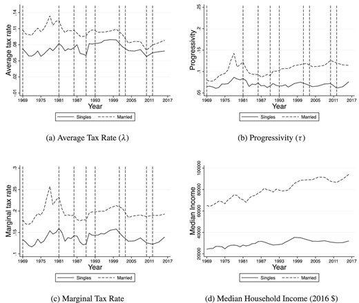
Estimation by household type: average tax rate, progressivity, marginal tax rate, and pre-tax median income. The average and marginal tax rates refer to the median household income for each household type and in each year. Vertical dashed lines: 1969, 1981, 1986, 1990, 1993, 2001, 2003, 2010, 2012 tax reforms.
Panel (a) of Figure 2 shows the evolution of the average tax rate, which is always higher for the median married couple than for the median single. For example, in 1969, the median single person has an income of about |${\$}$|24,000 and an average tax rate of about 7.3%, while the median married couple has an income of about |${\$}$|65,000 and an average tax rate of 10.8%. Over the period that we consider, the average tax rates for each group are at their lowest values in 2010, reaching 5.8 and 7.0% for singles and married couples, respectively. Their maximum values vary by demographic group and are 8.9% in 1998 for singles and 13.4% in 1978 for married couples.
Panel (b) of Figure 2 displays our progressivity parameter |$\tau$| over time. It is substantially higher for married couples. For singles, |$\tau$| varies from a minimum of 0.06 in 1971 to a maximum of 0.09 in 1978. For married couples, |$\tau$| varies between a low of 0.08 in 1970 and a high of 0.14 in 1978. Progressivity substantially flattens for singles after 1983, while it increases for married couples starting in 1987.
Panel (c) of Figure 2 shows the evolution of the marginal tax rate at the median income of each group every year. Like |$\tau$|, the marginal tax rate is substantially higher for married couples. The marginal tax rate for median singles varies between a low of 11.6% in 1972 and a high of 15.9% in 1981. The one for median couples varies between a low of 16.9 in 1971% and a high of 25.7% in 1978.
We now characterize the changes in the average tax rate and in progressivity for these groups by decade.
Seventies.
The seventies are characterized by a general upward trend in the average tax rate and progressivity for both married and single households. The average tax rate and progressivity evolve similarly for both groups; this finding is consistent with the absence of marital-status-specific reforms during the decade. During the seventies, median income is remarkably flat for singles, while it increases for couples. However, differences in median income only partially explain the differences in the average tax rate. In fact, the average tax rate at the median income decreases for both groups between 1974 and 1975 as a result of the Ford administration’s Tax Reduction Act of 1975, with the drop being larger for singles (1 percentage point) than for couples (0.6 percentage points), and with the drop in the associated median income being the same (about |${\$}$|2000 in 2016 units) for both groups. In addition, the average tax rate decreases between 1978 and 1979 because of Carter administration’s Revenue Act of 1978, with the drop in taxes being much larger for couples (1.7 percentage points) than for singles (0.4 percentage points) and with the associated decrease in median income being about |${\$}$|160 (in 2016 dollars) more pronounced for couples than for singles. Thus, the Tax Reduction Act of 1975 lowered taxes more for the median single household than for the median married household, while the opposite is true for the Revenue Act of 1978. In turn, progressivity, as measured by the parameter |$\tau$|, increases between 1972 and 1978 for both groups, and its increase for couples is double that for singles. Thus, the reforms just mentioned, the Nixon administration’s Tax Reform Act of 1969, and the Ford administration’s Tax Reform Act of 1976 result in increased progressivity, especially for median-income couples. As is consistent with the increases in both |$\lambda$| and |$\tau$|, the marginal tax rate at the median income of each group increases between 1972 and 1978, with the increase twice as large for couples (8 percentage points) than for singles (4 percentage points.)
Eighties.
In the first half of the eighties, all measures exhibit similar dynamics. In contrast, in the second half of the decade, they diverge by demographic group. The average tax rate declines for couples and singles during the first half of the decade. Specifically, after the Reagan administration’s ERTA of 1981, the average tax rate decreases between 1981 and 1983, increases slightly between 1983 and 1984, and is fairly stable between 1984 and 1985. Progressivity, as measured by |$\tau$| and the marginal tax rate at median income, drops sharply for all groups until 1983. After that, it declines slightly for couples, while it increases for singles until 1986. The drop in progressivity between 1981 and 1983 is related to the ERTA of 1981, while the increase between 1983 and 1986 could be due to the Reagan administration’s Deficit Reduction Act of 1984, which increased the EITC and is, thus, more relevant for singles than couples because singles are more likely to have lower incomes. The average tax rate for couples drops between 1986 and 1988 and is fairly stable between 1988 and 1990, while it rises for singles between 1986 and 1987 and then significantly declines until 1990. The Reagan administration’s Tax Reform Act of 1986 lowers the top tax rate and increases the bottom tax rate. This feature of the act may explain why couples, who have higher median income, face a decrease in the average tax rate, while singles, who have lower median income, face an increase in the average tax rate. The parameter |$\tau$| drops for both singles and couples between 1986 and 1987, in keeping with the Tax Reform Act of 1986, but after that, it substantially stabilizes for singles, while it starts increasing for couples, marking the start of a rise in |$\tau$| that lasts until 2000. The marginal tax rate drops for couples and singles between 1986 and 1990.
Nineties.
The nineties are characterized by a marked increase in progressivity for median couples, flat progressivity for median singles, and an increase in average tax rates for median couples and singles. The average tax rate increases for all groups between 1990 and 1992, as a consequence of the H.W. Bush administration’s Omnibus Budget Reconciliation Act of 1990. The average tax rate continues to increase for singles until 2000, while it declines slightly for couples between 1992 and 1994 and then increases until 2000. The Clinton administration’s Omnibus Budget Reconciliation Act of 1993 raised top tax rates for all demographic groups, but the act translated into an increase in effective taxes in 1993 only for median singles, while median married couples faced an increased tax rate starting in 1995. Progressivity, measured by |$\tau$|, rises markedly for median couples over the whole decade. The increase in progressivity is consistent with both the Omnibus Budget Reconciliation Act of 1990—which raised the top tax rate and expanded the EITC—and the Omnibus Budget Reconciliation Act of 1993—which raised the top tax rate. However, |$\tau$| declines for singles between 1991 and 1993 and increases only after 1996. This means that the Omnibus Budget Reconciliation Act of 1993 increased progressivity for median couples, but did not do so for median singles until 1996. The marginal tax rate increases steadily for median couples and singles between 1990 and 1999, reflecting the increases in |$\lambda$|, |$\tau$|, and real income.
Two-Thousands.
The first decade of the 21st century is characterized by a decrease in average tax rates and by heterogeneous dynamics in progressivity by demographic group. The average tax rate decreases for all demographic groups between 2000 and 2004, owing to the Bush administration’s tax cuts of 2001 and 2003. The tax rate then continues to decline for median singles but increases slightly for median couples until 2006. It then decreases for all groups between 2008 and 2010, due to the decline in median income during the Great Recession. Progressivity, measured by both |$\tau$| and the marginal tax rate, declines for all groups between 2001 and 2003, consistent with the Bush tax cuts of 2001 and 2003. The parameter |$\tau$| then increases for median couples and singles until 2010. The marginal tax rate increases between 2004 and 2008 but declines between 2008 and 2010. The increase in progressivity between 2004 and 2010 is due to several reforms during George W. Bush’s administration, including the JGTRRA of 2003 and the Working Families Tax Relief Act of 2004.
Twenty-Tens.
The period between 2010 and 2016 is characterized by an increase in the average tax rate for all demographic groups and by divergent paths for progressivity. The increase in tax rates is accompanied by the rebound in real median income after the Great Recession, which may explain why the average tax rate increases despite the tax reforms of 2010 and 2012, which extended the Bush tax cuts of 2003. The progressivity parameter |$\tau$| declines steadily for median married couples between 2010 and 2016, while it shows a V-shaped path for median singles, with |$\tau$| decreasing between 2010 and 2012 and increasing between 2012 and 2016, as |$\tau$| does. The marginal tax rate is substantially flat for median-income married couples, declines for median-income singles between 2010 and 2012, and then increases between 2012 and 2016. Progressivity decreases between 2010 and 2012, despite the Obama administration’s Tax Relief, Unemployment Insurance Reauthorization, and Job Creation Act of 2010, which increased the child tax credit and EITC. However, progressivity increases for singles between 2012 and 2016, consistent with the Obama administration’s American Taxpayer Relief Act of 2012, which raised the top tax rate.
6. A Structural Model of Couples and Singles to Evaluate the Effects of Various Tax Regimes
Looking at effective tax rates over time is interesting and important, but gives us only a limited sense of whether these tax changes are large or small. One way to determine whether they are sizeable is to check the extent to which they affect household behavior. To do so, we adopt an estimated dynamic quantitative model of couples and singles over the life cycle and use it to evaluate the implications of various tax regimes on outcomes such as participation, hours worked by the workers, labor income, and savings.
We adopt the model of Borella, De Nardi, and Yang (2023), which we re-estimate for the cohort born in 1941–1945 using the PSID and the Health and Retirement Study (HRS) dataset. Our model fits the historical data over the life cycle of this cohort very well and implies sensible labor supply elasticities by age, gender, and marital status.
Importantly, in our benchmark estimation, each year, households face the effective tax functions that we estimate from the PSID for that year (See Figure 2 for a summary). We, thus, assume that households have perfect foresight about future tax regimes.
In Section 7, we discuss some tax regimes in more detail, both from a historical standpoint and by describing the changes in our estimated tax functions. We then compare the outcomes from our estimated model when we keep each tax regime fixed for the duration of the households’ life cycle. Besides quantifying outcomes and, thus, providing a better sense of how substantial a tax change was, these comparisons are important because in the structural literature, it is common to ignore tax and policy variation over time and to pick one particular year to estimate one’s model. We show that because tax variation over time is large, the choice of assuming a constant tax regime over one’s entire estimation horizon is not an innocuous one.
In our model, a period is one year long. Single people meet partners, and married people might get divorced. These marital status changes occur exogenously. Every working-age person experiences wage shocks, and every retiree faces health, medical expenses, and lifespan risk. People in couples face the risk of both partners. Households can self-insure by saving and by choosing whether to work and how much to work (for both partners, in the case of couples) and when to retire. To be consistent with the data, we allow for human capital (in the form of learning by doing) to affect wages. We explicitly model Social Security, including its spousal and survival benefits, the differential tax treatment of married and single people, the progressivity of the tax system (including the EITC) as estimated by our tax functions, and old-age means-tested transfer programs, such as Medicaid and Supplemental Security Income (SSI), which we parsimoniously represent as an old-age consumption floor. We also model the changes in the tax and Social Security system over time. We report the model’s details in Appendix C.
Figure 3 reports our model-implied moments, data, and 95% confidence intervals (from the PSID) for our 1945 birth cohort. More specifically, it shows participation and hours worked by the workers for married and single men and women and net worth for couples and single men and women. The model fits the targeted data well, which is remarkable given that it is tightly parameterized: we have 448 targets and estimate 19 parameters. One aspect of the fit that could be improved is wealth accumulation around retirement: average wealth tends to keep increasing in the data while it peaks in the model. A potentially important explanation that we leave for future research is bequest motives (De Nardi, French, and Jones 2016; De Nardi et al. 2021 find them to be important during the retirement period).
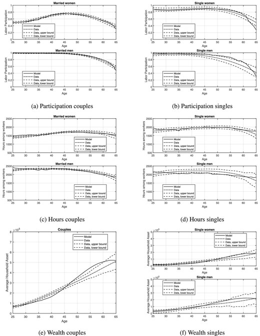
Model-implied participation (top panel), hours (middle panel), wealth (bottom panel), and average and 95% confidence intervals from the PSID. Time-varying taxation as in historical data.
Table 1 reports our model’s implied elasticities of participation and hours among workers with respect to an anticipated change to their own wage.6 It shows that the elasticity of participation of women is larger than that of men, that married men have the lowest elasticity of participation, that the elasticity of hours is different from that of participation, and that the elasticity of participation for all groups is largest around retirement age. Our elasticities are consistent with those in Blundell and Macurdy (1999), French (2000), Liebman, Luttmer, and Seif (2009), and Attanasio et al. (2018). This heterogeneity in elasticities underscores that the labor supply effects of a reform crucially depend on which groups are most affected by it.
Labor supply elasticity, temporary wage change, 1945 cohort. W: women, M: men.
| Participation | Hours among workers | |||||||
|---|---|---|---|---|---|---|---|---|
| Married | Single | Married | Single | |||||
| W | M | W | M | W | M | W | M | |
| 30 | 1.0 | 0.0 | 0.6 | 0.2 | 0.3 | 0.3 | 0.6 | 0.4 |
| 40 | 0.7 | 0.1 | 0.4 | 0.2 | 0.4 | 0.5 | 0.8 | 0.5 |
| 50 | 0.7 | 0.2 | 0.4 | 0.8 | 0.4 | 0.5 | 0.7 | 0.4 |
| 60 | 1.2 | 0.7 | 2.0 | 1.7 | 0.3 | 0.3 | 0.5 | 0.6 |
7. Selected Tax Reforms and Model Outcomes
We now turn to discussing nine tax reforms that represented major tax law changes, received extensive media coverage, and were sponsored by a president. The Online Historical Appendix compiles a history of all income tax reforms from 1962 to 2018 and presents more detail for each reform.
For each reform, we first describe the spirit of the law, its primary goals, and the context in which it takes place. Then, we show the effective tax functions in the year preceding the reform, the ones after the reform occurred, and those for the phase-in period, when one exists.7 To understand the effects of these tax regimes on household behavior, we then compare our model’s implications under the pre-reform tax regime with those under the post-reform regime. For clarity, in both cases, we hold each of these regimes constant over the households’ life cycle.
Finally, we turn to contrasting our estimated model’s implications for our benchmark in which taxes change every year (and households perfectly anticipate it) with our model’s implications under a scenario in which taxes remain constant at their 1969 levels. While this experiment is more complex to interpret (because taxes change every year and we have a dynamic model in which households react to both current and future changes), it is informative about the implications of ignoring tax variation over time, a choice often made by the literature calibrating or estimating structural models.
7.1. The Tax Reform Act of 1969
On April 21, 1969, President Nixon pushed for tax reform in a “special message to Congress,” saying “we must reform our tax structure to make it more equitable and efficient; we must redirect our tax policy to make it more conducive to stable economic growth and responsive to urgent social needs.” The 1969 Tax Reform Act was meant to achieve these goals. However, Nixon did not appear to like the final version of the bill passed by Congress. Nixon’s signing statement on December 30, 1969, was ambivalent, saying that “Congress has passed an unbalanced bill that is both good and bad. The tax reforms, on the whole, are good; the effect on the budget and the cost of living is bad” (Nixon 1969).
This reform was phased in gradually over the four years, between 1969 and 1973, and contained numerous income tax changes. First, it introduced a new rate schedule for singles that began in 1971. Until 1970, singles were taxed using the same schedule as married couples filing separately. Second, it established individual minimum taxes, which were a precursor to the modern Alternative Minimum Tax. Finally, it increased the personal exemption and the standard deduction.
The top four graphs of Figure 4 highlight the main features of this tax reform and its phase-in period. First, effective average and marginal tax rates vary over time, more so for singles than couples. For instance, the average tax rate for the median-income single (who earns |${\$}$|24,000, expressed in 2016 dollars, in 1969) decreases from 7.2% in 1969 to 5.6% in 1973. Similarly, the marginal tax rate for singles drops from 13.2% to 11.5%. The average tax rate for median-income couples (who earn |${\$}$|65,000, expressed in 2016 dollars in 1969) decreases only slightly, from 10.8% to 10.0% in 1973. In contrast, the marginal tax rate increases from 17.9% to 18.5% over the same time period. Second, the increases in personal exemptions and the standard deduction imply a higher effective income level below which the household pays no taxes (which generates the flat portion at zero in our graphs) that increases during the whole phase-in period. Third, the direction of these changes is not monotone over time. Taxes decrease every year until 1972 but go back up again in 1973 for both singles and couples. Fourth, the comparison of the 1973 and 1969 effective tax functions reveals that while average and marginal taxes decline at all income levels for singles, the patterns are different for couples, and the new tax regime implies more redistribution. Specifically, the average tax rate in 1973 is higher for couples with incomes above |${\$}$|155,000, and the marginal tax rate is higher for couples with incomes above |${\$}$|52,000.
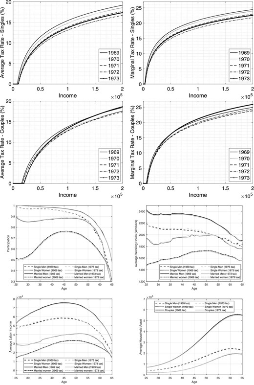
Comparing 1969 and 1973. Top two panels: tax rates. Bottom two panels: outcomes from structural model.
Next, we compare our model’s implications for the 1969 tax regime and the 1973 one. The bottom four panels of Figure 4 report four key model outcomes. The first three are participation, hours worked for the workers, and average labor income for four groups of people: single men and women and married men and women. The fourth displays the average wealth for couples and single men and women. These graphs show that singles, who now face lower average and marginal tax rates, work more. In contrast, married people, many of whom now face higher marginal tax rates, work and earn less. Within a couple, female labor supply is more elastic, especially at younger ages (owing to the effects of human capital accumulation). With respect to magnitudes, because the changes in tax rates are relatively small, so are changes in behavior. The participation rate of single people increases by 0.1 to 0.7 percentage points, depending on age and gender. The decrease in participation for married people ranges from 0.9 percentage points for young women to 0.2 for older men. The changes in hours and income go in the same direction and are also small. Moreover, singles save more (up to 3.5% more), and couples save less (up to 1.5% less).
7.2. The Inflation Period and 1978
The period between 1973 and 1978 was characterized by high inflation. The lack of tax bracket indexation to inflation, combined with the limited scope of the tax reforms during that period, resulted in much higher average and marginal tax rates than before and after. While inflation kept rising after 1978, effective taxation peaked that year, which is why we choose it.
The top four graphs of Figure 5 compare the 1973 and 1978 effective tax schedules. The first noticeable feature is that the changes in tax rates from 1973 to 1978 are much larger than those that took place during the previous 4-year period, during the Nixon reform. The second feature is that average and marginal tax rates increase substantially, except for those for lower-income couples. For instance, the average tax rate for the median-income single (who earns |${\$}$|27,000 in 1973) increases from 6.3% to 7.0%. Similarly, the median-income single’s marginal tax rate increases from 12.2% to 15.1%. The average tax rate for median-income couples (who earn |${\$}$|69,000 in 1973) increases from 10.5% to 12.5%, while their marginal tax rate increases from 18.5% to 24.9%.
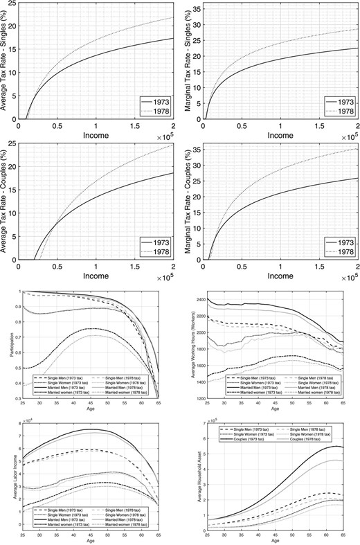
Comparing 1973 and 1978. Top two panels: tax rates. Bottom two panels: outcomes from structural model.
Next, we compare our model’s implications for the 1973 tax regime with those for the 1978 one. The bottom four panels of Figure 5 show that these two tax regimes have very different consequences on household behavior. An important feature is that the model’s implied participation of married women is much lower under the 1978 tax regime (9.4 percentage points at younger ages and 2.9 percentage points closer to retirement). In addition, hours worked by the workers are lower for all four demographic groups over most of their working period. For instance, over the first 10 years of the working period, hours drop by 5.1%, 2.4%, 4.5%, and 1.7% for married women, married men, single women, and single men, respectively. These drops in participation and hours translate into large reductions in labor income, of the order of 20.2%, 3.1%, 6.2%, and 2.1%, respectively. These decreases in labor income, in turn, result in substantial decreases in savings.
7.3. The Economic Recovery Tax Act of 1981
The impetus for the ERTA of 1981 was—as President Reagan argued during a televised address from the White House in February 1981—the federal government deficit, high inflation rates, high interest rates, high unemployment, burdensome regulations, low productivity growth, and excessive taxation of individuals. To tackle these issues, Congress passed the ERTA in August 1981.
This reform was phased in gradually between 1981 and 1984. It lowered income tax rates for all filing statuses and brackets. It also allowed a new deduction in computing adjusted gross income for two-earner married couples filing a joint return. The tax brackets, the personal exemption, and other tax elements were indexed to inflation starting in 1985.
The top four graphs of Figure 6 compare the 1980 and 1984 effective tax schedules and show that effective tax rates are lower in 1984, reflecting the goal of reducing “excessive taxation of individuals.” For instance, the average tax rate for the median-income single (who earns |${\$}$|27,000 in 1980) decreases from 7.6% to 6.7%. Similarly, the marginal tax rate for this category drops from 15.1% to 13.3%. The average tax rate for median-income couples (who earn |${\$}$|72,000 in 1980) decreases from 12.4% to 10.5%, while their marginal tax rate drops from 22.5% to 18.9%.
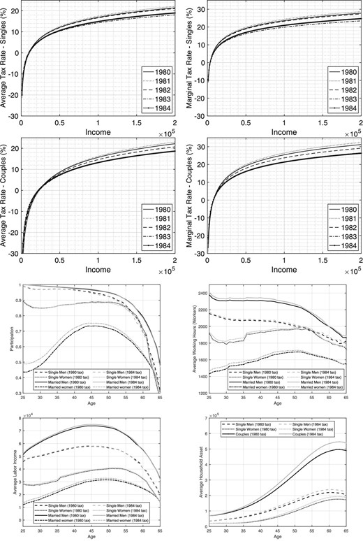
Comparing 1980 and 1984. Top two panels: tax rates. Bottom two panels: outcomes from structural model.
We now turn to our model’s implications for the 1980 tax regime and the 1984 one. The bottom four panels of Figure 6 show that these tax regimes have different implications for household behavior. As taxes drop, labor supply and savings increase. However, because the tax changes are a little smaller than those between 1973 and 1978, so are the household’s responses. For instance, the participation of married women increases by 4.4 percentage points at younger ages and 1.0 percentage points closer to retirement. In addition, hours worked by the workers increase for all four demographic groups over most of their working period. For instance, over the first 10 years of the working period, hours rise by 2.4%, 1.1%, 1.9%, and 0.7% for married women, married men, single women, and single men, respectively. These increases in participation and hours translate into higher labor income, of the order of 10.5%, 1.4%, 2.7%, and 0.8% for married women, married men, single women, and single men, respectively. These higher labor incomes, in turn, result in larger savings.
7.4. The Tax Reform Act of 1986
In the mid-1980s, President Reagan continued pushing the tax reduction effort. The 1986 Tax Reform Act was phased in between 1986 and 1988 and contained numerous provisions related to income taxes. First, it decreased the number of tax brackets and statutory tax rates. Second, it instituted a 2-year increase in the EITC and introduced a provision to address inflation in calculating the EITC. Finally, it increased the standard deduction and the personal exemption.
The top four graphs of Figure 7 compare the 1985 and 1988 effective tax schedules and show that effective tax rates are lower in 1988, reflecting Reagan’s continued goal of reducing taxation. The average tax rate for the median-income single (who earns |${\$}$|30,000 in 1985) decreases from 7.2% to 6.2%. Similarly, the median-income single’s marginal tax rate drops from 13.6% to 12.5%. The average tax rate for median-income couples (who earn |${\$}$|75,000 in 1985) decreases from 10.7% to 9.0%, while their marginal tax rate drops from 19.0% to 17.1%.
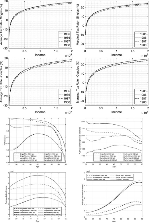
Comparing 1985 and 1988. Top two panels: tax rates. Bottom two panels: outcomes from structural model.
With respect to our model’s implications for these two tax regimes, the bottom four panels of Figure 7 reveal that in this case, the most noticeable changes occur for married women. More specifically, at younger ages, their participation increases by 1.3 percentage points, their hours worked, conditional on working, go up by 0.7%, and their income rises by 2.8%. As a result, the wealth of young married couples is 2.5% higher.
7.5. The Omnibus Budget Reconciliation Act of 1990
The Omnibus Budget Reconciliation Act (OBRA) of 1990 aimed at reducing the federal budget deficit. It was signed in November 1990 by President George H.W. Bush. The act took effect in 1991 and increased the individual income statutory tax rates, the alternative minimum tax rate, and payroll taxes. It also expanded the EITC and other low-income credits.
The top four graphs of Figure 8 compare the 1989 and 1991 effective tax schedules and show that this tax reform did increase effective taxation for both singles and couples, reflecting the goal of reducing the budget deficit. More specifically, the average tax rate for the median-income single (who earns |${\$}$|31,000 in 1989) increases from 6.4% to 8.8%. Similarly, the median-income single’s marginal tax rate rises from 12.3% to 15.4%. The average tax rate for median-income couples (who earn |${\$}$|80,000 in 1989) grows from 11.8% to 14.8%, while their marginal tax rate rises from 17.4% to 21.0%.
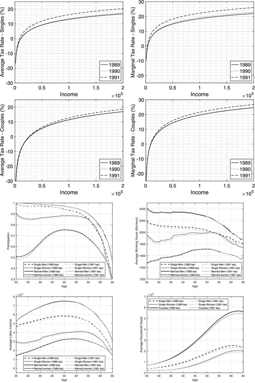
Comparing 1989 and 1991. Top two panels: tax rates. Bottom two panels: outcomes from structural model.
With respect to our model’s implications for these two tax regimes, the bottom four panels of Figure 8 show that this reform results in lower participation by young married and single women, lower hours for young married women and single people, and lower income and savings. More specifically, over the first 10 years of their working period, the participation of young married and single women drops by 1.9 and 0.9 percentage points, respectively. The hours of married women drop by 0.8%, those of single men by 1.2%, and those of single women by 2.3%. By contrast, income drops by 3.8% for married women, 1.6% for single men, and 2.6% for single women. Wealth for couples decreases by 1.4% and that of single men and women by 4.6% and 1.5%, respectively.
7.6. The Omnibus Budget Reconciliation Act of 1993
Soon after taking office in January 1993, President Clinton criticized the tax policy of his predecessor: “The big tax cuts for the wealthy, the growth in Government spending, and soaring health care costs all caused the Federal deficit to explode...while the deficit went up, investments in the things that make us stronger and smarter, richer and safer, were neglected...” (Clinton 1993b). Soon after, he also stated that: “in order to accomplish both increased investment and deficit reduction...spending must be cut and taxes must be raised” (Clinton 1993a).
The OBRA was signed in August 1993 and increased individual income tax rates retroactively, starting on January 1, 1993. Specifically, it raised the top tax rate, previously set at 31%, and imposed two new brackets with 36% and 39.6% tax rates. It also increased the Alternative Minimum Tax (AMT) exemption amounts and created a two-tiered tax rate structure for the AMT, replacing the pre-1993 24% AMT tax rate with 26% and 28% tax rates. Finally, OBRA extended the EITC to single workers with no children earning |${\$}$|9,000 or less per year.
We estimate no statistically significant changes in the tax parameters for singles and small but statistically significant changes in the parameters for couples. As a result, the estimated tax functions (and the model implications) for 1993 are very similar to those in 1992. Hence, we do not report them. The fact that there are no changes in singles’ taxes is consistent with the fact that OBRA contained provisions directed mostly at high-income taxpayers. For instance, the increase in the top tax rates affected singles earning more than |${\$}$|115,000 and couples earning more than |${\$}$|140,000. While the fraction of singles earning more than |${\$}$|115,000 is small, the fraction of couples earning more than |${\$}$|140,000 is relatively larger. This is why we observe no change for singles but statistically significant changes for couples.
7.7. The Economic Growth and Tax Relief Reconciliation Act of 2001 and the Jobs and Growth Tax Relief Reconciliation Act of 2003
President George W. Bush focused on the federal government budget surplus as a rationale for tax reform and tax cuts. The 2001 EGTRRA introduced a lower income tax bracket, reduced marriage penalties by increasing the joint standard deduction, and increased the child tax credit. This reform was phased in until 2006, and most of its provisions were meant to be temporary and expire at the end of 2010.
In 2003, President George W. Bush called for faster implementation of the changes set in motion by the 2001 EGTRRA. To this end, Congress passed the JGTRRA in May 2003 to make the previous reform’s tax cuts permanent and decrease income taxes further. The JGTRRA also accelerated many of the previous reform’s provisions and made them effective in 2003. In particular, it expanded the child tax credit and implemented the tax rate schedule and lower tax brackets and tax rates that were supposed to be in effect starting in 2006.
The top four graphs of Figure 9 compare the 2000 and 2006 effective tax schedules. The average tax rate for the median-income single (who earns |${\$}$|35,000 in 2000) decreases from 8.9% to 7.5%. Similarly, the median-income single’s marginal tax rate drops from 15.8% to 13.6%. The average tax rate for median-income couples (who earn |${\$}$|89,000 in 2000) decreases from 10.9% to 8.3%, while their marginal tax rate changes from 21.3% to 18.6%.
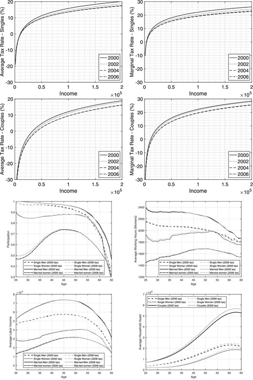
Comparing 2000 and 2006. Top two panels: tax rates. Bottom two panels: outcomes from structural model.
With respect to our model’s implications for these two tax regimes, the bottom four panels of Figure 9 show that this reform results in higher participation by young married and single women, higher hours and income for married and single women, and large increases in savings by all groups. More specifically, the participation over the first ten years of the working period by married and single women increases by 2.3 and 0.1 percentage points, respectively. Hours rise by 0.8% and 1.2% for the same groups. Their incomes go up by 4.6 and 1.7%, while the wealth of young couples is 3.8% higher and that of single women and men is 3.0% and 2.9% higher, respectively.
7.8. The Tax Relief, Unemployment Insurance Reauthorization, and Job Creation Act of 2010
The Great Recession motivated the Tax Relief, Unemployment Insurance Reauthorization, and Job Creation Act of 2010. President Obama wanted to avoid the automatic increase in tax rates caused by the expiration of the Economic Growth and Tax Relief Reconciliation Act of 2001 and the Jobs and Growth Tax Relief Reconciliation Act of 2003 (collectively known as the Bush tax cuts.) The 2010 Act temporarily prolonged the Bush tax cuts until the end of 2012, increased the Alternative Minimum Tax exemption, and provided a temporary payroll tax cut.
The top four graphs of Figure 10 compare the 2008 and 2012 effective tax schedules. They show that while the reform slightly raises the effective tax rates of couples with above median income, it decreases those of singles above a certain income threshold (|${\$}$|25,000 and |${\$}$|8,000 for the average and marginal tax rate, respectively.) As a result, the average tax rate for the median-income single (who earns |${\$}$|32,000 in 2008) decreases from 7.1% to 6.8%. Similarly, the median-income single marginal tax rate drops from 13.7% to 12.5%. The average tax rate for median-income couples (who earn |${\$}$|91,000 in 2008) goes from 8.6% to 8.5%, while their marginal tax rate increases from 18.8% to 19.5%.
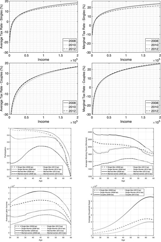
Comparing 2008 and 2012. Top two panels: tax rates. Bottom two panels: outcomes from structural model.
With respect to our model’s implications for these two tax regimes, the bottom four graphs of Figure 10 show that this reform results mainly in more hours worked by single people. More specifically, hours worked over the first 10 years of the working period go up by 1.4% for single women and by 0.7% for single men. The rest of the outcomes do not vary much.
7.9. The 1969 Tax Regime Compared with the Historically Realized Regimes
In this subsection, we investigate how household behavior would have evolved if households had faced the 1969 tax regime during their entire life cycle instead of facing the observed historical tax variation. Hence, we start by comparing the 1969 tax regime with the time-varying tax regime described in Figure 2. In particular, we assume that households have perfect foresight about the evolution of taxes over time.
Figure 11 shows that a fixed tax regime has very different implications for household behavior than those of our time-varying benchmark. Panel (a) shows that the 1969 tax regime implies higher participation by married people and lower participation by singles. For instance, the participation of young married women is 2.1 percentage points higher, while the participation of young single women is 0.3 percentage points lower. Panel (b) shows that the increase in participation by married people is accompanied by a rise in their hours worked. In particular, hours increase by 1.4% and 0.9% for young married women and young married men, respectively under the 1969 regime. The increase in participation and hours leads to higher labor income, as shown in Panel (c), which grows by 4.9% for young married women and by 1.2% for young married men. Finally, Panel (d) shows that the increase in couples’ income leads to a rise in their savings, which are 0.8% and 7.4% higher at younger and older ages, respectively.
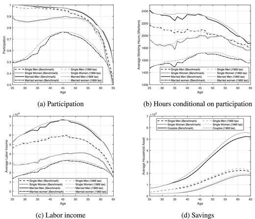
Comparing outcomes from our structural model with the observed variation in taxes (benchmark) with outcomes with a 1969 constant tax regime.
8. Conclusions
This paper estimates effective income tax functions from 1969 to 2016 for a representative decision unit, married couples, and singles. We find substantial variation in average tax rates, marginal tax rates, and income tax progressivity across time and household types. We also compile a detailed history of income tax reforms over the last 60 years and relate nine notable tax reforms to our estimated tax functions. Finally, we use an estimated, dynamic model of couples and singles to better evaluate to what extent different tax regimes lead to different behavior responses in labor market participation, hours worked, and labor income and savings over the life cycle for married and single men and women.
We document the changes over time in average and marginal tax rates and income tax progressivity. We first do so for a representative decision unit; that is, we do not distinguish between couples and singles. We find that average and marginal tax rates display similar trends. When average tax rates increase—as is the case in the seventies and nineties—the marginal tax rates grow. When average tax rates decrease—as in the eighties, two-thousands, and twenty-tens—marginal tax rates also fall.
Second, we study the same changes over time, conditional on family structure—that is, for couples and singles. We show that tax rates and progressivity have changed significantly over time because of both different economic circumstances and policy changes. While some reforms met the goal they were meant to achieve, others did not have the desired effects on tax rates and progressivity.
Third, we use our estimated structural model to evaluate to what extent these tax regimes affect key economic behaviors and hence to what extent it is important to model the evolution of tax changes over time. We find not only that these tax regime changes are frequent but also that many of them imply effective tax variation that generates very different economic outcomes. For example, the increase in effective taxation that occurred during the 1973–1978 high-inflation tax period significantly and negatively affected the participation of married women, the hours worked by single and married men and women, and their labor income and savings. The 1981 Reagan tax cut also affected these behaviors, although in the opposite direction and to a slightly smaller extent. Noticeable also are the 1986 Reagan tax cut, the 1990 George H.W. Bush. tax increases, and the George W. Bush tax cuts, which especially affected the participation of married women. Our model also predicts that the 2010 Obama tax cut increased hours worked by all four groups.
While we model tax changes over time, we assume perfect foresight. Given the frequency of these tax changes and the uncertainty surrounding the legislative process, it seems likely that economic decision-makers face a significant amount of uncertainty about the size and evolution of future taxes. While quantifying the effects of this uncertainty is very important, it makes for a major endeavor, and we leave it to future research.
Acknowledgments
This paper is based on the JEEA-FBBVA Lecture of the European Economic Association given virtually at FBBVA headquarters in Madrid in May 2023. The authors gratefully acknowledge support from the BBVA Foundation. De Nardi gratefully acknowledges support from NSF grant SES-2044748. We thank Marco Bassetto, Ellen McGrattan, Edward Nelson, Markus Poschke, and David Sturrock for their useful comments. The views expressed herein are those of the authors and do not necessarily reflect the views of the National Bureau of Economic Research, the CEPR, any federal government agency, the Federal Reserve Bank of Dallas, the Federal Reserve Bank of Minneapolis, or the Federal Reserve System. De Nardi is a Faculty Research Fellow of the CEPR and NBER.
Appendix A: Data
A.1 The PSID
The PSID is a longitudinal survey of U.S. families that started in 1968 to evaluate President Johnson’s War on Poverty. The original PSID sample included approximately 5,000 households divided into two subsamples: the Survey Research Center (SRC) sample, which was a representative sample of the U.S. population and consisted of around 3,000 families, and the Survey of Economic Opportunity (SEO) sample, which oversampled poor families and included approximately 2,000 families. We consider only the SRC sample.8
Data have been collected annually from 1968 to 1997 and biennially after. Income questions in the PSID are retrospective, which means that, for example, questions asked in the 2017 wave refer to income for the 2016 calendar year.
We use each PSID wave available between 1970 and 2017 (corresponding to the tax years 1969–2016) to estimate time-specific tax functions. While PSID data are available for 1967 and 1968 as well, they miss information on the transfers that we need to construct our estimation inputs, and thus we do not use them.
A.2 Income Definitions and Components
Our measure of household income is the sum of the income received by the head of the household and the spouse (if present).
Pre-tax income is defined as the sum of all monetary income received by the head of the household and the spouse (or by the head only, if single) in a given tax year. It includes labor income; the asset part of the income from farm, business, roomers, and the like; income from rent received; interest and dividend income; and transfer income, which includes (Aid to Dependent Children later turned into Aid to Families with Dependent Children and currently Temporary Assistance for Needy Families), Social Security benefits, income from retirement pay, pensions or annuities, unemployment benefits and worker’s compensation, alimony and child support received, help from relatives, Supplemental Security Income (SSI), income from other sources, and other welfare income. Post-tax income is defined as pre-tax income minus the federal income tax liability, which includes capital gains rates, surtaxes, AMT, and refundable and nonrefundable credits, as computed by TAXSIM (the NBER microsimulation program to compute taxes).
We convert all nominal variables into real terms using the CPI-U and 2016 as our base year.
A.3 Taxes
Information about federal income taxes paid is provided directly by the PSID up to 1991. After that date, we compute taxes by using the NBER’s TAXSIM (we extend the program written by Kimberlin, Kim, and Shaefer 2015).9 We calculate post-tax income as pre-tax income minus taxes.
A.4 Imputation of Medical Expenses
Medical expenses are needed to compute tax liabilities. We compute them using the approach of Borella, De Nardi, and Yang (2023) as follows.
For years before 1999, data on medical expenses and charitable contributions are not available and must be imputed, as they may be deducted from gross income (if the household chooses to itemize). We impute them by regressing the sum of the two items for the pooled years 1999–2016 and using these regression coefficients to compute fitted values for the years prior to 1999. To perform this regression we include demographic and income variables, such as family size, employment status of the head and spouse, if present, state of residence, wages, pensions, other incomes, education, number of children, age, and marital status. Then, we add an error term to that prediction to tackle the attenuation in the variance of the distribution of the imputed values, following the procedure in David et al. (1986), and French and Jones (2011). Considered in more detail, the procedure is as follows. After regressing the sum of the two items on the vector of observables for the sample of heads who choose to itemize, we compute both the predicted value and the residual. So we have |$\textit {deduc} = z\beta + \varepsilon$|. Second, for each household i for which |$\textit {deduc}$| is observed, we calculate the predicted value |$\widehat{\textit{deduc}}_i = z_i\beta$| and the residual |$\hat{e}_i ={\textit deduc}_i-\widehat{\textit {deduc}}_i$|. Third, we sort the predicted value |$\widehat{\textit {deduc}}_i$| into deciles and keep track of all values of |$\hat{e}_i$| within each decile. Next, for every individual j with missing |$\textit {deduc}$|, we impute |$\widehat{\textit {deduc}}_j = z_j\beta$|. Then, we impute |$\hat{e}_{\!j}$| for households with missing |$\textit {deduc}$| by finding a random individual i in the non-missing sample with a value of |$\widehat{\textit {deduc}}_i$| in the same decile as |$\widehat{\textit {deduc}}_j$| and set |$\hat{e}_j=\hat{e}_i$|. The imputed value of |$\textit {deduc}$| is |$\widehat{\textit {deduc}}_j + \hat{e}_j$|.
A.5 Marital Status
In Section 5, we estimate tax functions by marital status. We distinguish between singles, married couples, and cohabiters. We only consider to be “married,” couples who are legally married and can thus file their taxes jointly, while cohabiting households are composed of two unmarried people who live together. By law, cohabiters cannot file their taxes jointly—only legally married couples can—and must file their taxes as singles. Until 1983 the PSID did not distinguish between married couples and cohabiters, so we observe cohabiters only from the 1983 wave onward.
A.6 Sample Selection
Our initial sample consists of 161,321 observations for households from the SRC subsample of the PSID.
Table A.1 describes our sample selection for estimating effective tax functions for the representative decision unit. We first drop all observations with non-positive income, as we cannot compute logs for those. Then, we drop the observations for the years 1967 and 1968 because they do not contain crucial information about transfers that we need to construct our income definitions. This leaves us with 154,669 observations. Then, we trim the sample to exclude observations with pre-tax income below the 0.5th and above the 99th percentile in each year. Subsequently, we drop observations with missing values of either log pre- or post-tax income and observations with plainly incorrect values of the income component variables. This leaves us with 150,501 observations.
Sample selection for representative decision unit.
| Sample | Selected out | Selected in |
|---|---|---|
| Initial sample | 161,321 | |
| Positive income | 1,092 | 160,229 |
| 1969–2016 | 5,560 | 154,669 |
| After income trimming | 2,248 | 152,421 |
| Has all values of income | 1,914 | 150,507 |
| Has consistent income | 6 | 150,501 |
| |$|\text{DFBETA}|<1$| | 1 | 150,500 |
We further clean additional outliers using the DFBETA procedure (see for instance Bollen and Jackman 1985). That is, before estimating our tax functions, we run year-by-year regressions of log post-tax income on log pre-tax income to compute DFBETAs. The DFBETAs cleaning methodology focuses on one coefficient—in our case, the coefficient on the logarithm of pre-tax income in equation 4—and computes the difference between the estimated coefficients when a certain observation is included and when it is excluded. It then scales that difference by the estimated standard error of the coefficient. We remove observations with DFBETA greater than 1 (as done by Bollen and Jackman 1985), which imply that a particular observation is eliminated when it shifts the estimated coefficient by at least one standard error. Our final sample for the representative decision unit consists of 150,500 observations.
Table A.2 describes the sample selection for estimating effective tax functions by household type. The procedure is similar to the one for the representative decision unit, the only difference being that we perform income trimming by year and household type. The final samples consist of 50,561 observations for singles, 93,166 for married couples, and 6,845 for cohabiters.
Sample selection by household type.
| Sample | Selected out | Selected in |
|---|---|---|
| Initial sample | 161,321 | |
| Positive income | 1,092 | 160,229 |
| 1969–2016 | 5,560 | 154,669 |
| After income trimming | 2,204 | 152,465 |
| Has all values of income | 1,870 | 150,595 |
| Has consistent income | 5 | 150,590 |
| Singles | ||
| |$|\text{DFBETA}|<1$| | 1 | 50,561 |
| Married Couples | ||
| |$|\text{DFBETA}|<1$| | 0 | 93,166 |
| Cohabiters | ||
| |$|\text{DFBETA}|<1$| | 17 | 6,845 |
Appendix B: Tax Function Fit
Among others, Heathcote, Storesletten, and Violante (2017) and Fleck et al. (2021) show that our log-linear tax function provides a good approximation of the federal income tax system in the United States. We corroborate this finding by dividing log pre-tax income in 50 bins; for each of those bins, we compute the average of log pre- and post-tax income at 50 quantiles. Figure B.1 reports the results for 6 years and shows that this relationship is approximately log-linear. The remaining PSID waves display very similar patterns.

Log post-tax income as a function of log pre-tax income. Post-tax income is defined as pre-tax income minus federal income taxes. Each dot corresponds to a quantile of the log pre-tax income distribution and the corresponding average log post-tax income. The dashed line is the 45-degree line.
Appendix C: Structural Model
As our model comes from Borella, De Nardi, and Yang (2023), we follow its exposition closely. Net worth |$a_{t}$| earns a rate of return r. Our model period is one year long. There are three stages in one’s life: a working stage (ages 25–61), an early retirement stage (ages 62–65), and a retirement stage (age 66 to the maximum age of 99).
During the working stage, single and married individuals choose how much to work and save and face wage shocks. Married people face divorce shocks, and single people might meet partners and get married. Wages are a function of one’s human capital (which is endogenously accumulated while working) and are affected by shocks.
We model (and estimate) available time to be split between working and leisure and allow it to depend on one’s gender and marital status. We interpret it as net of home production, child care, and elderly care that one has to perform whether working or not (and that is not easy to outsource). All workers have to pay a fixed cost of working, which depends on their age, gender, and marital status. It represents the cost of commuting, getting ready for work, making arrangements for being able to work, and so on.
Single women and married people have children, and their number depends on maternal age and marital status. We allow for both time costs and monetary costs of raising children. The time costs affect one’s available time for working and enjoying leisure. The monetary costs enter our model in two ways: they affect consumption through equivalent scales, and working mothers have to pay child care costs that depend on the age and number of their children and on their own earnings. Hence, child care costs are a normal good: women with higher earnings pay for more expensive child care.
During the early retirement stage, people still experience wage shocks, but single people don’t get married anymore, and couples no longer divorce.10 If they claim Social Security, they can no longer work. Couples claim Social Security jointly.
During the first year of the retirement stage, those who have not already claimed Social Security do so and stop working. People face health shocks, out-of-pocket medical expenses, and mortality shocks. Thus, each married person faces the risk of their spouse dying, in addition to their own death. Mortality risk and medical expenses depend on gender, age, health status, and marital status.
C.1 Preferences
Let t be age, with people entering at age 25 and dying by age 99. Given that we only have one cohort, t indexes both age and time.
Households discount the future at rate |$\beta$|. The superscript i denotes gender, with |$i=1, 2$| being a man or a woman, respectively. The superscript j denotes marital status, with |$j=1, 2$| being single or being in a couple, respectively.
Each single person has preferences over consumption and leisure, and the period flow of utility is given by the standard CRRA utility function
where |$c_t$| is consumption, |$\eta ^{i,j}_t$| is its equivalent scale for couples and |$\eta ^{i,1}_t$| is the one for singles, and |$l_t^{i,j}$| is leisure, which is given by
where |$L^{i,j}$| is available time, net of home production, which can be different for single and married men and women. The functional form we use for it is
where we normalize L to 112 hours a week and estimate |$FL^{i,j}$| using our structural model. The term |$n^i_t,$| is hours worked, and |$I_{n^i_t}$| is an indicator function that equals 1 when hours worked are positive.
The term |$\Phi ^{i,j}_t$| is the fixed time cost of working, which depends on gender, marital status, and age. It assumes the following functional form, whose parameters we estimate using our structural model:
We assume that couples maximize their joint utility function
Note that for couples, |$\eta ^{i,j}_t$| does not depend on gender and |$j=2$|.
C.2 Human Capital and Wages
We define human capital, |$\bar{y}^i_t$|, as one’s average past earnings at each age [see equation (C.11) for a formal definition]. It is therefore a function of one’s initial wages (and schooling to the extent that it is reflected in one’s wages) and subsequent labor market experience and wages, and not just of experience measured as the amount of time one has previously worked. Our definition has two important benefits. First, it respects the previous findings that the returns to experience depend on one’s education, and thus human capital and earnings (Blundell et al. 2016a; Costa Dias, Joyce, and Parodi 2020). Second, it allows us to use only one state variable to keep track of both human capital and Social Security contributions, thereby keeping our framework manageable.
Wages have two components: a deterministic function of age, gender, and human capital |$e_{t}^{i}(\bar{y}^i_t)$| and a persistent shock |$\epsilon _{t}^{i}$| that evolves as follows:
The product of |$e_{t}^{i}(\cdot )$| and |$\epsilon _{t}^{i}$| determines one’s effective hourly wage per hour.
C.3 Marriage and Divorce
During the working period, the probability that a single person gets married at the beginning of next period depends on age, gender, and wage shock: |$\nu _{t+1}(\cdot )=\nu _{t+1}(i, \epsilon ^i_{t})$|.
To allow for assortative mating conditional on meeting a partner, we make it so that the probability of meeting a partner p with wage shock |$\epsilon _{t+1}^{p}$| is
We assume random matching over wealth |$a_{t+1}$| and average accumulated earnings of the partner |$\bar{y}_{t+1}^{p}$|, conditional on the partner’s wage shock. Thus, we have
A working-age couple can be hit by a divorce shock that depends on age and the wage shock of both partners: |$\zeta _{t+1}(\cdot )=\zeta _{t+1}(\epsilon _{t}^{1},\epsilon _{t}^{2})$|. If the couple divorces, they split their wealth equally (we experimented with different asset splits with very similar results). We abstract from alimony.
C.4 Costs of Raising Children and Running a Household
We keep track of both the total number of children and their age as a function of mothers’ age and marital status. The term |$f^{0,5}(i,j,t)$| is the number of children age 0–5, and |$\tau _c^{0,5}$| is the child care cost for each child in that age group. Similarly, |$f^{6,11}(i,j,t)$| is the number of children age 6–11, and |$f^{0,5}(i,j,t)$| is the corresponding child care cost for each child. We use our structural model to estimate these costs.
C.5 Medical Expenses and Death
Once they reach age 66, we endow people with a distribution of health that depends on their marital status and gender. After that, they face survival, medical expenses, and health shocks. Health status |$\psi _{t}^i$| can be either good or bad and evolves according to a Markov process |$\pi _t^{i,j}(\psi _t^i)$| that also depends on age, gender, and marital status. Medical expenses |$m_t^{i,j}(\psi _{t}^i)$| are a function of age, gender, marital status, and health. Survival probabilities |$s_{t}^{i,1}(\psi _{t}^{i})$| are a function of age, gender, marital status, and health.
C.6 Initial Conditions
We take the fraction of single and married people at age 25 and their distribution over the relevant state variables (wealth, human capital, and wage shocks, the latter two being for each of the spouses in the case of couples) from the PSID for our cohort.
C.7 Government
Each household in our model faces the effective time-varying tax rates that it experienced in the data and that we estimate from the PSID as discussed in the main body of the paper and in several appendices. We allow our effective tax rates to depend on marital status and age for our cohort (and thus time). Taxes paid are a function of total income Y as described in equation (1) in the main body of the paper.
The government uses a proportional payroll tax |$\tau ^{SS}_t$|, up to a Social Security cap |$\tilde{y}_t,$| to help finance old-age Social Security benefits, which are a function of average past earnings (or human capital, as discussed in Section C.2). We also allow the payroll tax and the Social Security cap to change over time, as in the data. We thus assume that the tax changes were anticipated by the households. The insurance provided by Medicaid and SSI in old age is represented by a means-tested consumption floor, |$\underline {c}(j)$|, as in Hubbard, Skinner, and Zeldes (1995).11
C.8 Recursive Formulation
We compute nine value functions for the following groups and stages of life.
C.8.1. The Value Function of Working-Age Singles
The value function of a working-age single depends on the person’s age t, gender i, wealth |$a_{t}^{i}$|, persistent earnings shock |$\epsilon _{t}^{i}$|, and human capital |$\bar{y}_{t}^{i}$|:
subject to equation (C.1) and
The expectation of the value function for next period if one remains single integrates over one’s wage shock next period. If one gets married, it also integrates over the distribution of the partner’s state variables. The value function |$\widehat{W}^c$| is the person’s discounted present value of utility once he or she is in a married relationship with someone with given state variables (see Appendix C.8.7). equation (C.11) describes the evolution of human capital, measured as average accumulated earnings (up to the Social Security earnings cap |$\tilde{y}_{t}$|) and in which |$t_0=25$|.
C.8.2. The Value Function of Singles during the Early Retirement Stage
The recursive problem for someone who has claimed Social Security at age |$tr$| is
subject to equations (C.9), (C.12), and
The term |$SS(\bar{y_{r}}^i, tr)$| is a function of the income that the single person earned during his or her working life |$\bar{y}_{r}^i$| and claiming age |$tr$|.
Let |$N^{s}(t, i, a_{t}^{i},\epsilon _{t}^{i},\bar{y}_{t}^{i})$| denote the value function of a person during the early retirement period who has not yet claimed benefits:
subject to equations (C.1), (C.7), (C.9), (C.11), (C.12), (C.13), and
Let |$V^{s}(t, i, a_{t}^{i},\epsilon _{t}^{i},\bar{y}_{t}^{i})$| denote the value function for a person during the early retirement stage who has not yet claimed and who, at the beginning of each period, chooses whether to claim, where |$D_{t}^{i}$| is an indicator function for claiming
C.8.3. The Value Function of Retired Singles
The value function of a retired single with health |$\psi _{t}^{i}$|, average realized lifetime earnings |$\bar{y}_{r}^i$|, and Social Security claiming age |$tr$| is
subject to equations (C.9), (C.12), (C.15), and
The term |$B(a_{t},Y_{t}^{i},\psi _{t}^{i},\underline {c}(j))$| represents old-age means-tested government transfers (such as Medicaid and SSI) that ensure a minimum consumption floor |$\underline {c}(j)$|.
C.8.4. The Value Function of Couples during the Working Period
The value function of a married couple at this stage depends on both partners’ state variables, where 1 and 2 refer to gender and |$j=2$|:
subject to equations (C.1), (C.7), (C.8), (C.11), and
The expected value of the couple’s value function is taken with respect to the conditional probabilities of the wage shocks for each of the spouses (we assume independent draws). The expected values for the newly divorced people are taken using the appropriate conditional distribution for their own wage shocks. The term |$\zeta _{t+1}(\cdot )$| represents the probability of divorce.
C.8.5. The Value Function of Couples during the Early Retirement Period
The recursive problem for couples that have claimed Social Security at age |$tr$| is
subject to equations (C.9), (C.16), (C.12), and
The variable |$Y_{t}$| represents Social Security spousal benefits: married people receive the highest amount between their own benefit and half of their spouse’s benefit.
The value function of a couple that has not yet claimed benefits is
subject to equations (C.1), (C.7), (C.11), (C.25), (C.27), and
The value function of a married couple during the early retirement stage that has not yet claimed Social Security benefits is
C.8.6. The Value Function of Couples during Retirement
During this stage, the married couple’s recursive problem (|$j=2$|) depends on each spouse’s health shocks |$\psi _{t}^{i}$|, and there are survival shocks |$s_{t}^{i,2}(\psi _{t}^{i})$|. We assume that the health shocks of each spouse are independent of each other and that the death shocks of each spouse are also independent of each other:
subject to equations (C.9), (C.12), (C.23), (C.29), and
Survivors collect benefits based on the higher amount between their own contributions and those of their deceased spouse [equation (C.34)].
C.8.7. The Value Functions of Individuals in Couples
We have to compute the joint value function of the couple to appropriately compute joint labor supply and savings under the married couple’s available resources. However, when computing the value of getting married for a single person, the relevant object for that person is his or her discounted present value of utility in the marriage. We thus compute this object for person of gender i who is married with a specific partner.
Let |$\hat{c}_{t}(\cdot )$|, |$\hat{l}_t^{i,j}(\cdot )$|, |$\hat{a}_{t+1}(\cdot )$|, and |$\widehat{D}_{t}(\cdot )$| denote, respectively, the optimal consumption, leisure, saving, and claiming decision for an individual of gender i in a couple with a given set of state variables. During the working period, we have
During the early retirement period, we have
During the retirement period, we have
where |$s_{t}^{p,j}(\psi _{t}^{p})$| is the survival probability of the partner of the person of gender i.
C.9 Estimation
We estimate the model by adopting a two-step estimation strategy (as Gourinchas and Parker 2002). In the first step, we use data on the initial distributions at age 25 for our model’s state variables and estimate or calibrate those parameters that can be cleanly identified outside our model.
In the second step, we use the method of simulated moments. We normalize the time endowment for single men and estimate 19 model parameters (|$\beta$|, |$\omega$|, (|$\phi _0^{i,j}, \phi _1^{i,j}, \phi _2^{i,j}$|), (|$\tau _c^{0,5}, \tau _c^{6,11}$|), |$L^{i,j}$|). The data that inform the estimation of the parameters of our model are composed of the following 448 moments:
Labor market participation of married and single men and women age 25–65
Hours worked, conditional on working, for married and single men and women age 25–65
Wealth for couples and single men and women age 26–65.
Footnotes
We do so by constructing a representative decision unit using household-level data and, within the household, summing the incomes of the one or two adults present and computing the corresponding taxes.
As discussed in Appendix A, we trim our sample to exclude the top 1% and bottom 0.5% of pre-tax income by year to reduce heteroskedasticity.
It is worth pointing out the parameter |$\tau$| is unaffected by any normalization. For |$\lambda$|, we provide both normalized and un-normalized estimates in our replication package, as well as the formula expressing it as a function of the normalization.
After 1985, tax brackets, personal exemptions, standard deductions, and many other tax elements are indexed to inflation. In particular, until 2018, indexation is based on the CPI-U. We also use the CPI-U to convert nominal variables into real ones for estimation. After 2018, indexation is based on the chained CPI-U (C-CPI-U.)
In principle, married couples could file as married but filing separately. However, doing so entails the loss of many deductions and exemptions. As a result, the vast majority of couples (about 97%) chooses to file jointly.
To compute these elasticities, we temporarily increase the wage for only one age and one group at a time (married men, married women, single men, or single women) by 5%. While we do not compensate this wage change, a temporary change in wage of this size is very small compared to a family’s lifetime earnings and consumption.
We report the results for the representative decision unit in Online Appendix F.
We follow Kimberlin, Kim, and Shaefer (2015) also to compute mortgage interest and the related itemized deduction in each year.
Only |$1\%$| of couples get divorced and |$4\%$| of singles get married between ages 62 and 72 in the HRS data for our 1945 cohort.
Borella, De Nardi, and French (2018a) discuss Medicaid rules and observed outcomes after retirement.
Notes
The editor in charge of this paper was Nicola Pavoni.
