


Abstract
We study the optimal progressivity of personal income taxes in a general equilibrium overlapping generations model where individuals are exposed to idiosyncratic shocks to labor productivity and health status over the lifecycle. Our results—based on a calibration to the US economy—indicate that both, the presence of health risk and the available insurance institutions, have a strong effect on the optimal level of tax progressivity. Given the fragmented and non-universal health insurance system in the US, a welfare maximizing income tax system is substantially more progressive than the current US income tax. The higher progressivity provides additional redistribution and social insurance, especially for unhealthy low income individuals who have limited access to health insurance. When exposure to health risk is removed or reduced by introducing more comprehensive health insurance systems, we observe large decreases in the optimal level of income tax progressivity, and the optimal tax system resembles findings from the previous literature. These findings highlight the importance of accounting for the unique characteristics of health risk and the design of the health insurance system when characterizing optimal income taxes.
1. Introduction
The US income tax system is progressive and plays a key role in shaping the income distribution across households and over time. Traditionally, the optimal taxation literature has investigated optimal progressivity levels in heterogeneous agent models with income risk and incomplete markets (Varian 1980; Conesa and Krueger 2006; Heathcote et al. 2017). In particular, Heathcote et al. (2017) find that in their model, the optimal income tax system is less progressive than the existing system in the US. What is currently missing from the discussion on optimal tax progressivity is the consideration of health risk and limited access to health insurance, which have both been identified as a prominent source of risk and lifecycle inequality (Capatina 2015; De Nardi, Pashchenko, and Porapakkarm 2018). The purpose of this paper is to revisit the optimal tax progressivity in a new analytical framework that explicitly models health risk and institutional features of the US health insurance system.
The presence of health risk as an additional source of agent heterogeneity, in addition to income risk, introduces a new channel that influences the traditional roles of a progressive income tax system.1 In the context of the US policy settings where the health insurance system is fragmented and only provides partial health insurance, we find that the optimal income tax system is more progressive in order to provide a sufficient level of redistribution and social health insurance to unhealthy low income individuals who have limited access to health insurance. However, when more inclusive health insurance systems such as “Medicare for all”—we refer to this as universal public health insurance (UPHI)—are introduced, we observe large decreases in the optimal level of income tax progressivity. When the exposure to health risk is already largely mitigated through the UPHI system, not much additional social health insurance is required from the progressive income tax system and therefore the optimal level of progressivity decreases. Our findings highlight the importance of accounting for health risk and insurance arrangement when characterizing the optimal progressive income system.
We show that the progressive income tax system has two channels that increase welfare: one that reduces post tax earnings inequality and the other that provides support to low income individual who have limited access to health insurance. The former traditionally appears in any models without market mechanisms to hedge against initial skill endowments; meanwhile, the latter appears in this model where the health insurance system fails to protect the poor from high health expenditure. We refer the latter as “health-related tax progressivity” channel.
We next formulate a quantitative model of the US economy and use it to simulate how this health-related tax progressivity channel plays out in a general equilibrium framework. Our quantitative model is an overlapping generations economy model with a consumption, savings, labor, and insurance choice and household heterogeneity due to idiosyncratic shocks to labor productivity and health status. More specifically, our benchmark model combines the key ingredients of a standard heterogeneous agent model with idiosyncratic income risk (Bewley 1986; Huggett 1993; Aiyagari 1994) and ingredients of a heterogeneous agent model with health risk (Jeske and Kitao 2009). Importantly, our model incorporates important institutional features of the US health insurance system, including private individual health insurance (IHI) plans, employer sponsored group health insurance (GHI) plans, Medicaid for the poor, and Medicare for retirees. Individuals have limited access to certain types of health insurance plans and rely partially on precautionary saving and labor supply to smooth consumption spending over the lifecycle. Health expenditure shocks affect household utility via reducing funds available for purchasing final consumption goods. In this incomplete markets setting, the simultaneous presence of both income and health risks shapes the distributions of income, wealth, and consumption. Progressive income taxes and public health insurance simultaneously serve as policy tools that provide social insurance against income and health risks.
We calibrate the model to US data. Our benchmark model is capable of matching labor supply, asset holdings, consumption, health expenditures, and health insurance take-up rates over the lifecycle similar to observable US data. We next use the model to quantify the optimal level of income tax progressivity, using ex-ante expected utility of a newborn agent in a stationary equilibrium as the welfare criterion.
We use a two parameter polynomial tax function following Benabou (2002) to approximate the US income tax code.2 The optimal income tax system is highly progressive and comprises a tax break for income up to |${\$}$|8,800 followed by a steep increase in the marginal tax rate to |$20\%$| at the income level of |${\$}$|20,000. The marginal tax rate then increases further to over |$30\%$| for income above |${\$}$|70,000 and to over 35 percent for income above |${\$}$|150,000. The zero tax bracket at the low end of the income distribution is mainly driven by the high demand for social health insurance for the low income, unhealthy population who has limited access to the US health insurance system. The high tax rates at the upper end of the income distribution are required to meet the financing needs of government spending programs. The optimal income tax system found in our model has much higher marginal tax rates than the optimal ones reported in the previous literature that largely abstract from health risk and insurance (Conesa and Krueger 2006; Heathcote et al. 2017).
In order to compare the progressivity levels of the different income tax regimes, we follow Suits (1977) and compute a tax progressivity (Suits) index, which is a Gini coefficient for income tax contributions by income group.3 The US income tax system in the benchmark model has a Suits index of 0.122. The optimal US tax system is substantially more progressive with a Suits index of 0.218, which reduces income inequality significantly. The after-tax-income Gini coefficient decreases from 0.352 in the benchmark economy to 0.320 after the progressivity level is optimized. Moderate welfare gains of |$0.102\%$| of compensating lifetime consumption at the aggregate level can be realized. These gains are mainly driven by large welfare gains of low and middle income individuals who dominate the welfare losses of the higher income group.
Our results highlight the quantitative importance of the social health insurance role of progressive income taxes. More specifically, in our incomplete markets setting with income and health risks, the redistribution of income via the progressive income tax system provides implicit insurance for both, income and health risks. The latter is a new channel that is missing in prior studies that abstract from modeling health risk. In our model with exogenous health expenditure shocks, unhealthy individuals are more likely to have lower income as health shocks correlate with labor productivity. In addition, lower income workers are less likely to be matched with employers who offer group health insurance and therefore have higher out-of-pocket medical expenditures. Many of these lower income individuals are uninsured as they are not poor enough to qualify for Medicaid and not rich enough to buy private health insurance on their own or through their employers.4 The “poor working class” benefits strongly from the optimized tax system in terms of welfare gains as they benefit from the expanded zero tax threshold. As a result, these individuals are in a better position to smooth consumption fluctuations due to uncertainty in health expenditure and income shocks. The consumption of the uninsured indeed increases under the optimal income tax system. This novel mechanism emphasizes the importance of accounting for health risk and the institutional features of the US healthcare system, when studying the optimal design of a progressive income tax system in the US context.
In order to isolate quantitatively the importance of the health-related tax progressivity channel, we take a step back and consider a framework where health risk is no longer present in the model. The demand for health insurance becomes redundant in this reduced model.5 The social health insurance role of the progressive income tax system—the health-related tax progressivity channel—is therefore removed from the model. Our quantitative analysis based on this model indicates that the optimal income tax system is much less progressive than the US status quo tax system and exhibits similar features of the optimal progressive tax code found in Conesa and Krueger (2006). We conclude that health risk, as another source of agent heterogeneity, in addition to income risk, plays an important role in shaping the optimal level of progressivity of the US income tax system. The absence of health risk diminishes the social insurance function of the redistributive income tax system and results in a much lower level of tax progressivity in the optimum.
We next investigate how different designs of the US health insurance system affect the optimal design of the progressive income tax system. We focus on two alternative health insurance scenarios: (i) a system where all public and private health insurance are eliminated and individuals rely exclusively on self-insurance (No health insurance), and (ii) a system with Medicare for all workers and retirees that we refer to as universal public health insurance (UPHI). Under the no health insurance scenario, the optimal level of tax progressivity increases significantly and exhibits a much higher tax progressivity (Suits) index of 0.369. Conversely, when an inclusive UPHI system is introduced, the optimal level of tax progressivity decreases significantly. The reason is that the UPHI system already removes a large portion of the health spending risk. In particular, with a coinsurance rate of |$30\%$| the tax break at the lower end of the income distribution decreases significantly to |${\$}$|200, and the marginal tax rates imposed on top earners are lower at approximately |$32\%$| for income over |${\$}$|150,000. The tax progressivity (Suits) index decreases to 0.07 under the UPHI system. Thus, the introduction of UPHI significantly reduces the residual demand for social health insurance provided by the progressive income tax system.
Furthermore, the optimal level of tax progressivity varies significantly across alternative designs of UPHI coinsurance. There is indeed an inverse relationship between UPHI coinsurance rate and optimal tax progressivity. When the UPHI system is more generous with lower coinsurance rates, the optimal tax system becomes less progressive. When the UPHI coinsurance rate is set to zero, namely full health insurance, the optimal tax system resembles a proportional tax schedule found in Conesa and Krueger (2006). When the UPHI system is less generous with higher coinsurance rates, the optimal tax system becomes more progressive and looks more similar to the one found in Heathcote, Storesletten, and Violante (2017). This result again confirms a strong connection between the available health insurance arrangement and the optimal tax progressivity in a model with health and income risks.
As robustness checks we relax several modeling assumptions. Our main results are robust to alternative values of preference parameters, the addition of health-dependent preferences similar to De Nardi, French, and Jones (2010), the addition of state and local taxes as well as corporate taxes similar to Guner, Lopez-Daneri, and Ventura (2016), changes to the labor productivity process, and a higher minimum consumption floor.6
The paper is structured as follows. Section 2 presents the quantitative model. Section 3 describes our calibration strategy. Section 4 describes our experiments and quantitative results. Section 5 is devoted to extensions and sensitivity analyses. Section 6 concludes. The appendices provide additional results from the benchmark model, the model description of the model without health shocks, more details about the data we used for calibration, and a description of the computational algorithm we used to solve the model.
Related Literature.
In a seminal paper, Varian (1980) shows analytically how social insurance can be provided via a progressive tax system. Building on this insight, there exists a large quantitative literature on the optimal design of the progressive income tax code. Examples include Conesa and Krueger (2006), Erosa and Koreshkova (2007), Chambers, Garriga, and Schlagenhauf (2009), Krueger and Ludwig (2016), Stantcheva (2017), Heathcote et al. (2017), and McKay and Reis (2021). However, none of these papers studies progressive income taxes in combination with health insurance policies as our paper does.
Our paper uses an incomplete markets macroeconomic models with heterogeneous agent as pioneered by Bewley (1986) and extended by Huggett (1993) and Aiyagari (1994). The Bewley-type model has been applied widely to quantify the welfare effects of providing social insurance against income risk (Hansen and Imrohoroglu 1992; İmrohoroğlu, İmrohoroğlu, and Joines 1995; Golosov and Tsyvinski 2006; Heathcote, Storesletten, and Violante 2008; Conesa, Kitao, and Krueger 2009; Huggett and Parra 2010). We contribute to this literature a quantitative model with health risk and health insurance arrangement. We highlight that the presence of health-related spending adds a new channel, which affects the social insurance role of a progressive income tax system.
Our work contributes to a growing macro-public finance literature that focuses on health shocks and healthcare policy. Early studies usually view health shocks as health expenditure shocks (Palumbo 1999; Jeske and Kitao 2009). Recent studies endogenize health expenditure (Jung and Tran 2007; Scholz and Seshadri 2013; Jung and Tran 2016; Yogo 2016; Cole, Kim, and Krueger 2019; Fonseca et al. 2021). However, none of these papers analyze the social insurance role of progressive income taxes, which is the focus of this paper. In addition, there is an analogy to the literature that emphasizes the complementarity between progressive taxes and education policies, dated back to an influential work by Bovenberg and Jacobs (2005). Recently, Krueger and Ludwig (2016) provide a quantitative analysis. Our quantitative model contains a similar fiscal externality as it has a similar modeling approach. Different from theirs, our paper aims to better understand the interaction of optimal progressive taxes with health insurance policies.
Finally, our paper is connected to the literature on high marginal tax rates for top income earners. Diamond and Saez (2011) advocates for taxing labor earnings at the high end of the distribution at high marginal rates in excess of |$75\%$|. Badel, Huggett, and Luo (2020) assess the consequences of increasing the marginal tax rate on US top income earners using a human capital model. Guner, Lopez-Daneri, and Ventura (2016) analyze the effectiveness of progressive income tax systems in raising tax revenue, and Kindermann and Krueger (2022) show that high marginal labor income tax rates are an effective tool for social insurance in an overlapping generations model. Different from these studies, we base our analysis on a new model where health risk is an additional source of heterogeneity. We show that high marginal tax rates at the top are an essential component of the optimal progressive tax system.
2. The Quantitative Model
We formulate a baseline quantitative model based on an overlapping generations (OLG), incomplete market model with uninsurable idiosyncratic income risk in the spirit of Conesa and Krueger (2006), augmented by exogenous ex-post heterogeneity in health status due to health risk and a fragmented health insurance system due to the US institutional settings. In the model, the utility maximizing households are exposed to exogenous labor productivity shocks and health expenditure shocks, while having limited access to private or public health insurance contracts. The profit maximizing firm produces a final consumption good and government provides Social Security, Medicare, Medicaid, and consumption insurance for low income households.
2.1. Demographics, Endowments, and Preferences
Individuals are born and become economically active at the age of 21 and live to a maximum of J periods. Individuals are allowed to work for a maximum of JW periods. In each period, individuals of age j face an exogenous survival probability πj(εh) that depends on their exogenous health state εh. Due to the mortality risk, individuals will leave accidental bequests.
In addition, the population grows exogenously at an annual rate |${\mathit {n}}$|. We assume stable demographic patterns, so that age j agents make up a constant fraction μj of the entire population at any point in time. The relative sizes of the cohorts alive μj and the mass of individuals dying |$\tilde{\mu }_{j}$| in each period (conditional on survival up to the previous period) can be recursively defined as
where |$\textit {years}$| denotes the number of years per model period and μj(εh) is the mass of individuals with health εh.
In each period, households are endowed with one unit of time that can be used for work ℓ or leisure. Conditional on labor force participation, a household earns before-tax wage income yj = w × ej(ϑ, εn, εh) × nj at age j, where w is the wage rate, and ej is a labor productivity endowment that depends on age j, a permanent income group ϑ, an idiosyncratic productivity shock εn, and idiosyncratic health state εh. Labor shocks follow a Markov process with transition probability matrix Πn. Parameter |$\bar{n}_{j}$| denotes age-dependent fixed cost of working.
The period utility function |$u(c_{j},\ell _{j};\bar{n}_{j}\cdot 1_{[0\le n_{j}]})$| depends on consumption (c), leisure (ℓ), and labor force participation status, which is only equal to 1 if labor supply exceeds a minimum threshold.
2.2. Health Status, Expenditure, and Insurance
Individuals are different in their health status εh, which evolves exogenously over their life time. Specifically, health status follows a Markov process that depends on age and the permanent income group. The conditional transition probabilities are elements of matrix Πh(j, ϑ). A specific level of health expenditures m(j, ϑ, εh) is linked directly to health status and fluctuates accordingly. In addition, the permanent income type and age also affect the fluctuation of exogenous health expenditure. It is important to note that health affects consumption and utility indirectly via exogenous shocks to health expenditure and labor productivity in the household budget constraint in this baseline model (namely the budget channel). In an extension, we will relax this assumption and allow for the exogenous health state to directly affect household preferences (namely a morbidity channel).
Workers can buy two types of private health insurance policies: a group health insurance plan (GHI) via their employer or an individual health insurance plan (IHI). In the US setting, GHI is not only more strictly regulated than IHI but also subsidized via the US tax system via tax deductible premium payments. This makes GHI a particularly attractive form of health insurance. Agents are required to buy insurance before the realization of their health state and the associated medical expenditures and insurance needs to be renewed each period. GHI can only be bought by workers who receive a GHI offer from their employer. Let εGHI be a binary random variable that indicates the state of the GHI offer from the employer. The GHI offers follow a Markov process summarized as the two state transition matrix ΠGHI(j, ϑ) that depends also on age and an individuals permanent income group. A fraction ψ ∈ [0, 1] of the insurance premium for GHI, |$\text{prem}_{j}^{\text{GHI}}$|, is paid for by the employer, the remainder of the premium |$\widehat{\text{prem}}_{j}^{\text{GHI}}=(1-\psi )\text{prem}_{j}^{\text{GHI}}$| is tax deductible and paid by the worker. This premium is group rated so that insurance companies are not allowed to screen workers by health.7 If a worker is not offered GHI by their employer, then the worker can buy IHI. In this case, the insurance premium is not tax deductible and the insurance company screens the workers by age and health status, |$\text{$\text{prem}$}^{\text{IHI}}(j,\epsilon ^{h})$|.8
There are two public health insurance programs in the US health insurance system: Medicaid for the poor workers and Medicare for retirees. To be eligible for Medicaid, agents are required to pass an income and asset test. After retirement (j > JW + 1) all agents are covered by public health insurance, which is a combination of Medicare and Medicaid. Let inj denote the insurance state, which can take on the following values:
The out-of-pocket health expenditure oj(m) depends on health insurance status
where 0 ≤ γin ≤ 1 are the coinsurance rates of the different insurance types.
2.3. Insurance Companies
We abstain from modeling insurance companies as profit maximizing firms and simply allow for a premium markup ω. Since insurance companies in the individual market screen customers by age and health, we impose separate clearing conditions for each age-health type, so that premiums, premIHI(j, h), adjust to balance
where |$x_{j,-\epsilon ^{h}}$| is the state vector for cohort age j not containing health state εh since we do not want to aggregate over the health state vector εh in this case. The clearing condition for the group health insurances is simpler as only one price, premGHI, adjusts to balance
where |$\omega _{j,h}^{\text{IHI}}$| and ωGHI are markup factors that determine loading costs (fixed costs) and γIHI and γGHI are coinsurance rates. The respective left-hand-sides in the above expressions summarize aggregate payments made by insurance companies, whereas the right-hand-sides aggregate the premium collections one period prior. Since premiums are invested for one period, they enter the capital stock and we therefore multiply the term with the after tax gross interest rate R.
2.4. Technology and Factor Prices
The production sector is modeled by a representative firm that uses physical capital K and effective labor services N to produce output. The representative firm solves the following maximization problem:
taking the rental rate of capital q and the wage rate w as given. Capital depreciates at rate δ in each period.
Similarly to Jeske and Kitao (2009), we assume that the firm offering GHI to its workers subsidizes a fraction ψ of the premium cost. The firm passes these costs on to its employees by lowering the efficiency wage. To ensure the zero profit condition the firm subtracts the cost cE from the wage rate, which is just enough to cover the total premium cost of the firm. The effective wage rate received by the household with a GHI offer is therefore |$\widehat{w}=(w-1_{[\text{$\epsilon $}^{\text{GHI}}=1]}\times c_{E}).$| The zero profit condition implies that the wage reduction equals
In this scenario, high productivity workers effectively pay higher contributions toward financing the employer contribution to GHI as their wage deductions are larger in absolute terms. The remaining share of the GHI premium |$\widehat{\text{prem}}{}^{\text{GHI}}=\left(1-\psi \right)\times \text{prem$^{\text{GHI}}$}$| is income tax deductible and paid by the worker directly.
2.5. Government and Fiscal Policy
The government has the following fiscal activities.
Spending Programs.
The government runs five main spending programs: Social Security, Medicare, Medicaid, Social Transfers, and general government consumption. Social Security benefits are available only to the retirees after the eligibility age (j > JW). The benefit payment is determined by the average earnings history of a permanent income type |$\bar{y}^{\vartheta }$|. Retiring households are also eligible for Medicare after age j > JW at which point they start paying a Medicare premium premMCare every period. The surplus/deficit of Social Security and Medicare are given by
Medicaid is a public health insurance program for the poor. Working households are eligible for Medicaid payments if they pass the income and asset tests |$y_{j}<\bar{y}^{\text{MAid}}$| and |$a_{j}<\bar{a}^{\text{MAid}}$|, respectively. Social Security, Medicare, and Medicaid are included into the overall government budget constraint.9 Social Transfers bSI is a social insurance program that targets low income earners to guarantee a minimum consumption level |$\underline{c}$|. Finally, general government consumption CG is a residual (unproductive) government spending program.
Taxes.
The government raises revenues by imposing various taxes on income, consumption, and assets. This includes a progressive income tax |$T^{y}(y_{j}^{\text{T}})$| on taxable income |$y_{j}^{\text{T}}$|, which is the sum of labor income and capital interest income net of some deductibles as described in the next section. In addition, the government collects payroll taxes |$T^{{\rm SS}}(y_{j}^{{\rm SS}};\, \bar{y}^{{\rm SS}})$| and |$T^{{\rm MCare}}(y_{j}^{{\rm SS}})$| for Social Security and Medicare, respectively. The tax base for these payroll taxes |$y_{j}^{{\rm SS}}$| is defined as labor income minus GHI premiums. GHI premiums can be deducted from the progressive income tax base as well as the payroll tax base. In addition, the payroll tax for Social Security is proportional but capped at the maximum taxable earnings of |$\bar{y}^{{\rm SS}}$|. Finally, the government taxes consumption at a rate of τc and bequests at a rate of τBeq.
The progressive income tax schedule is modeled via a parametric function |$\tilde{\tau }(y^{\text{T}})=y^{\text{T}}-\lambda \times (y^{\text{T}})^{(1-\tau )}$|, where |$\tilde{\tau }(y^{\text{T}})$| denotes tax revenue as a function of taxable income yT, τ is the progressivity parameter, and λ is a scaling factor to match the US income tax revenue. This tax function is fairly general and captures the common cases:
This tax function has a long tradition in public finance (Musgrave 1959; Kakwani 1977) and was implemented into a dynamic setting by Benabou (2002) and more recently used in Heathcote et al. (2017). This tax function is flexible and can be used to model the transfer programs. Note that, Heathcote et al. (2017) abstract from modeling government transfer programs explicitly, but allow negative income taxes to act as implicit government transfers. We instead model the US institutional details of government transfer program explicitly via Social Security, Medicare, Medicaid, and Social Transfers. To avoid double counting, we impose a non-negative income tax restriction
This non-negative restriction eliminates all government transfers embedded in the tax function.
Budget Balancing.
The government budget constraint is given by
where surplus = surplusSS + surplusMCare is the combined surplus/deficit of Medicare and Social Security. The government adjusts the progressive income tax to balance its budget.
2.6. The Household Problem
In the model, we distinguish between workers and retirees.
Workers.
The state vector of a worker at a particular age is defined as |$x_{j}=\lbrace \vartheta ,a_{j},\text{$\text{in}_{j}$},\epsilon _{j}^{n},\epsilon ^{h},\epsilon _{j}^{\text{GHI}}\rbrace \in \lbrace 1,2,3\rbrace \times R^{+}\times \lbrace 0,1,2,3\rbrace \times \lbrace 1,2,3,4,5\rbrace \times \lbrace 1,2,3,4,5\rbrace \times \lbrace 0,1\rbrace$|, where ϑ denotes the permanent income group of no-high-school, high-school, and college types, aj denotes the beginning-of-period assets, inj denotes the health insurance state, |$\epsilon _{j}^{n}$| denotes the labor shock, and εh denotes the exogenous health state, and |$\epsilon _{j}^{\text{GHI}}$| is the employer (with group health insurance) matching shock. After the realization of the state variables, agents simultaneously chose from their choice set
where cj is consumption, ℓj is leisure, aj+1 are asset holdings for the next period, and inj+1 is the health insurance state for next period in order to maximize their lifetime expected utility. All choice variables in the optimization problem are functions of the state vector but we suppress this notation in order to not clutter the exposition. The household problem of the working household can be recursively written as
where β is a time preference factor, πj(εh) is the age and health state dependent survival probability, w is the market wage rate, r is the interest rate, o(mj) is out-of-pocket medical spending, and premin is the insurance premium paid. The indicator functions are defined as 1[true] = 1 and 1[false] = 0. Accidental bequests bBeq are redistributed to surviving households in a lump-sum fashion.10 Labor income |$y_{j}^{n}$|, total taxable income |$y_{j}^{\text{T}}$|, and payroll tax eligible income |$y_{j}^{ss}$| are defined as
where private GHI premiums are tax deductible as are out-of-pocket health expenses that exceed |$7.5\%$| of adjusted gross income.11
Consumption is taxed with rate τc, lump-sum bequests bBeq are taxed at rate τBeq and the remaining taxes are defined as
where Ty is a progressive income tax function of taxable household income |$y_{j}^{\text{T}}$|, τSS is the social security payroll tax levied on “social security wages”—essentially wages minus GHI premiums—and an upper contribution limit of |$\bar{y}^{{\rm SS}}$|, and |$T^{{\rm MCare}}$| is a Medicare payroll function with the same tax base but without an upper limit.12 Social transfers are defined as
and ensure a minimum consumption floor |$\underline{c}$| after medical expenses and taxes are paid for. A household consuming at the lower bound cannot save into the next period or purchase private insurance.
Average past labor earnings for each permanent income group ϑ follow
where |$\boldsymbol{x}\left(\vartheta \right)$| is the mass of households belonging to permanent income group ϑ.
Retirees.
Households can stop working at any time. Households retire at age j > JW at which point they receive Social Security benefits and qualify for Medicare.13 The state vector of a retiree at a particular age is defined as xj = {ϑ, aj, εh} ∈ {1, 2, 3} × R+ × {1, 2, 3, 4, 5}. The household optimization problem reduces to
where taxable income |$y_{j}^{\text{T}}$| is defined as
For retirees out-of-pocket expenses plus Medicare premiums that exceed 7.5% of gross income are tax deductible.14 Social insurance transfers are defined as
Since we force every retired individual into the combined Medicare/Medicaid program, the social insurance transfers include the Medicare premium.
Aggregation.
We denote |$\boldsymbol{x}\equiv \lbrace j,\, x_{j}\rbrace$| as the augmented state vector including age j and |$\Lambda \left(\boldsymbol{x}\right)$| is the measure of households with state |$\boldsymbol{x}$|, which incorporates the relative cohort sizes μj.
2.7. Competitive Equilibrium
The competitive equilibrium of the model with exogenous health spending risk is defined as follows. Given the transition probability matrices |$\lbrace \Pi _{j}^{n},\Pi _{j}^{h},\Pi _{j,\vartheta }^{\text{GHI}}\rbrace _{j=1}^{J}$| for ϑ ∈ {1, 2, 3}, the survival probabilities |$\lbrace \pi _{j} (\epsilon ^{h})\rbrace _{j=1}^{J}$| and the exogenous government policies exogenous government policies |$\lbrace T_{j}^{y},b_{j}^{\text{SI}},b_{j}^{{\rm SS}} \rbrace _{j=1}^{J}$| and |$\lbrace \tau ^{c},\tau ^{{\rm SS}},\tau ^{{\rm MCare}},\text{prem}^{{\rm MCare}},\gamma ^{{\rm MCare}},\gamma ^{\text{MAid}},C_{G}\rbrace ,$| a competitive equilibrium is a collection of sequences of distributions |$\Lambda \left(\boldsymbol{x}\right)$| of household decisions |$\lbrace c(\boldsymbol{x}),\ell (\boldsymbol{x}),a(\boldsymbol{x}),\text{in}\left(\boldsymbol{x}\right)\rbrace ,$| aggregate stocks of physical capital and effective labor services {K, N}, factor prices {w, q, R}, and insurance premiums {premIHI(j, εh), premGHI} such that:
|$\left\lbrace c\left(\boldsymbol{x}\right),\ell \left(\boldsymbol{x}\right),a\left(\boldsymbol{x}\right),in\left(\boldsymbol{x}\right)\right\rbrace$| solves the consumer problem (8, 9) ,
- the firm first order conditions hold$$\begin{eqnarray} w & = \frac{\partial F\left(K,N\right)}{\partial N},\\ q & = \frac{\partial F\left(K,N\right)}{\partial K},\\ R & = 1+q-\delta =1+r, \end{eqnarray}$$
- markets clear(16)$$\begin{eqnarray} K&=\int a(\boldsymbol{x})+\text{Prem}^{\text{GHI}}\left(\boldsymbol{x}\right)+\text{Prem}^{\text{IHI}}\left(\boldsymbol{x}\right)d\Lambda (\boldsymbol{x}) \end{eqnarray}$$(17)$$\begin{eqnarray} N&=\int e(\boldsymbol{x})\left(1-\ell (\boldsymbol{x})\right)d\Lambda (\boldsymbol{x}).\\ B^{\text{Beq}} & = \sum \limits _{j=1}^{J}\tilde{\mu }_{j}\int a_{j}(x_{j})d\Lambda (x_{j}), \end{eqnarray}$$
- the aggregate resource constraint holds$$\begin{eqnarray} C_{G}+\int \left(c\left(\boldsymbol{x}\right)+m\left(\boldsymbol{x}\right)+a\left(\boldsymbol{x}\right)\right)d\Lambda \left(\boldsymbol{x}\right)=Y+\left(1-\delta \right)K, \end{eqnarray}$$
the government programs clear so that (5),(6), and (7) hold,
the budget conditions of the insurance companies (2) and (3) hold, and
- the distribution is stationary$$\begin{eqnarray} (\mu _{j+1},\Lambda (x_{j+1}))=T_{\mu ,\Lambda }(\mu _{j},\Lambda (x_{j})), \end{eqnarray}$$where Tμ, Λ is a one period transition operator on the measure distribution$$\begin{eqnarray} \Lambda (\boldsymbol{x^{\prime }})=T_{\Lambda }(\Lambda (\boldsymbol{x})). \end{eqnarray}$$
3. Calibration
We calibrate the model to match data of the US economy between 1999 and 2009. Macroeconomic data moments include capital accumulation, patterns of labor supply, and health insurance take-up rates over the life cycle. For the calibration we distinguish between two sets of parameters: (i) externally selected parameters, and (ii) internally calibrated parameters. Externally selected parameters are estimated independently from our model and are either based on our own estimates using data from the Medical Expenditure Panel Survey (MEPS) or estimates provided by other studies. The model unit is an individual that we calibrate using information from the male and female heads of Health Insurance Eligibility Units (HIEU), which is a subset of a household in MEPS and comprises |$44\%$| women.15
We summarize these external parameters in Table 1. Internally calibrated parameters are assigned values so that model-generated data match a given set of targets from US data. These parameters are presented in Table 2. Model generated data moments and target moments from US data are juxtaposed in Table 3.16
3.1. Demographics, Endowments, and Preferences
Demographics.
We model households from age 21 to age 95. One model period is defined as 5 years, which results in J = 15 model periods. A typical individual works for nine periods and retiree for six periods. Once the individual enters period Jr+1 = 9, corresponding to the age of 65, she is forced to retire. We set the population annual growth rate to |$\mathit {n}=0.01$|, and we take the age and health specific survival probabilities π(h(εh)) from İmrohoroğlu and Kitao (2012) shown panel [8] of Figure 1. For the purpose of survival probabilities, we distinguish between healthy and sick individuals. The nature of exogenous health states εh is described in Section 2.2.
![Data input: exogenous health state process and health spending. Healthy is defined as an individual reporting either Excellent, Very Good, or Good health. Sick is defined as Fair or Poor health. Panels [1]–[4] show the average medical spending per age group (20–24, 25–29, 30–34, ...), self-reported health status, and permanent income group (no high school, high school, or college and higher). Panel [5] shows the average out-of-pocket health expenditures by age group and permanent income type. Panel [6] shows the medical spending distribution of the model period of 5 years. Panel [7] shows the self-reported health states by age group. The survival probabilities in panel [8] are from İmrohoroğlu and Kitao (2012), who base their estimates on data from the Health and Retirement Study and life table estimates in Bell and Miller (2005). Data source is MEPS 1999–2009. The observational unit is the head of a Health Insurance Eligibility Unit (HIEU), which is a subset of a household. We apply population weights.](https://oup.silverchair-cdn.com/oup/backfile/Content_public/Journal/jeea/21/5/10.1093_jeea_jvad010/2/m_jvad010fig1.jpeg?Expires=1750198579&Signature=mZIbAeh7aIr1eL096~HqAzLehdMuJ5CGB0GNI5OoBTE79ABfbngoSXyTHDfiokx7vRIgYdtaIlFG~5jpv2NbmMo2hc1UxREl9Yu36CWoOs43fw5y-xJPETMNuM6BcsWwdZ-m9S~6SvGfffkJ8RF9ncozG0DIG0V9EHUK-W7bYZvxBozy5oQ1wkb5n4cKpqMCVoFNvt1jvSyxOx4jSrO77tZnm9DN5z~y1ZGhlHg1iFvUbE6-9jWqf1TB3w4p3uHseeKIo~FYYuSvrQ7LuhPf4VB4MSeOiefGeO~uYWtJMR7dSp3dbevBSnk9ZleuEnFpK~OuaPMB1MuCfH6BpCFgow__&Key-Pair-Id=APKAIE5G5CRDK6RD3PGA)
Data input: exogenous health state process and health spending. Healthy is defined as an individual reporting either Excellent, Very Good, or Good health. Sick is defined as Fair or Poor health. Panels [1]–[4] show the average medical spending per age group (20–24, 25–29, 30–34, ...), self-reported health status, and permanent income group (no high school, high school, or college and higher). Panel [5] shows the average out-of-pocket health expenditures by age group and permanent income type. Panel [6] shows the medical spending distribution of the model period of 5 years. Panel [7] shows the self-reported health states by age group. The survival probabilities in panel [8] are from İmrohoroğlu and Kitao (2012), who base their estimates on data from the Health and Retirement Study and life table estimates in Bell and Miller (2005). Data source is MEPS 1999–2009. The observational unit is the head of a Health Insurance Eligibility Unit (HIEU), which is a subset of a household. We apply population weights.
Endowments.
We model the labor income process by assuming that labor productivity at age j is driven by an age, income group, and stochastic health state dependent component |$\bar{e}_{j}(\vartheta ,\, h(\epsilon ^{h}))$| and a residual stochastic labor shock component |$\epsilon _{j}^{n}$|
The permanent income group is defined as the education level ϑ in the first model period.
Using 1999–2009 MEPS data, we construct cohort adjusted and bias corrected wage profiles for each education–health subgroup (ϑ, h(εh)) limiting the sample to heads of health insurance eligibility units (HIEU) with labor incomes larger than |${\$}$|400.17 We distinguish between three permanent educational groups
and two health states
These are standard definitions for healthy and sick in the health macro literature. Panel [3] in Figure 4 depicts the fraction of healthy individuals. We then deflate hourly wage observations with the urban CPI and remove cohort effects. Following the procedure in Casanova (2013) and Rupert and Zanella (2015), we subsequently estimate a selection model to remove the selection bias that is typically associated with wage observations to get an average wage offer rate for each (ϑ, h(εh)) subgroup. We finally smooth the wage profiles with a second degree polynomial in age.18
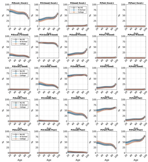
Data input: conditional health status Markov transition probabilities. The estimates of the conditional health state transition probabilities are based on an ordered logit model. Data source is MEPS 1999–2009, heads of HIEU, population weighted.
![Calibration targets: Labor market and insurance percentages. Labor participation (5 year averages) in Panel [1] and average work hours in Panel [2] are calibration targets that determine the fixed cost of labor participation as well as the consumption versus leisure weight in the utility function. Panels [3]–[6] show the fraction of individuals with individual health insurance (IHI), employer provided group health insurance (GHI), as well as the recipients of Medicaid and Medicare. Data source is MEPS 1999–2009, heads of HIEU, population weighted.](https://oup.silverchair-cdn.com/oup/backfile/Content_public/Journal/jeea/21/5/10.1093_jeea_jvad010/2/m_jvad010fig3.jpeg?Expires=1750198579&Signature=oOPtg4SVWkWkLsY-3cev2tFUenSutZBD4rDkrAUSU6cCnd64HQRORyZ89swB~MNdAL8q2lo82yMBLJK8lRRRa72r0xnZMf3ctCpYigKApvnA32o1kMti6TiL1q4iIJVC5VTTI5WF7wU693SzSieDLtavU-s7cPpyUV27zTVjd5qAwEoaHmo08U-ieou7TofFpfb2FNHftj60qwJLUZnCvCXxwLXQxHtBtnxwZYUi9Z2IJoye9O4L5M7yrC6PcEjdkZMQFqqggso7kYT5fz002KbRYFdELCTfjzJFeY7Phl1eOvHgq4hqYdyKSupJzXiL-t-22t7vQsjlgp23N4vXKQ__&Key-Pair-Id=APKAIE5G5CRDK6RD3PGA)
Calibration targets: Labor market and insurance percentages. Labor participation (5 year averages) in Panel [1] and average work hours in Panel [2] are calibration targets that determine the fixed cost of labor participation as well as the consumption versus leisure weight in the utility function. Panels [3]–[6] show the fraction of individuals with individual health insurance (IHI), employer provided group health insurance (GHI), as well as the recipients of Medicaid and Medicare. Data source is MEPS 1999–2009, heads of HIEU, population weighted.
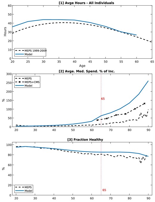
Model performance: Lifecycle profiles. These are not calibration targets. Data source is MEPS 1999–2009, heads of HIEU, population weighted.
The stochastic component is modeled as an auto-regressive process so that
with persistence parameter ρ and a white-noise disturbance |$\varepsilon \sim N\left(0,\sigma _{\varepsilon }^{2}\right)$|. To calibrate the stochastic component εn, we use ρ = 0.977 and |$\sigma _{\epsilon }^{2}=0.0141$| based on estimates in French (2005), who uses Panel Study of Income Dynamics (PSID) data and controls for cohort effects and health states. We approximate the joint distribution of the persistent and transitory shocks using a five-state first-order discrete Markov process following Tauchen and Hussey (1991).
Preferences.
We specify period utility as
We set the relative risk aversion parameter σ to 3, and the intertemporal discount factor β to 0.99 to match the capital–output ratio target in equilibrium. Labor is chosen from a grid n ∈ {0, nmin , …, nmax }, where the minimum amount of non-zero labor possible is nmin = 300 hours per year. The fixed cost of working |$\bar{n}_{j}$| is set to match the average labor participation rate per 5-year age group from MEPS. The consumption intensity parameter η is 0.272 to match average labor hours of the working population. The resulting Frisch labor elasticity is state dependent and the average Frisch elasticity of age j individuals can be calculated based on individuals that are working as19
where |$1_{[0\le n_{j}(x_{j})]}$| is an indicator function equal to 1 if an individual is working. Our calibration results in average Frisch elasticities between 1.19 for younger workers and 1.51 for older workers.20 Section 5.3 provides robustness checks using parameter values for σ and η that result in slightly lower Frisch elasticities. Finally, in our model the intertemporal elasticity of substitution (IES) is |$\frac{1}{3}.$|21
3.2. Health Status, Health Expenditure, and Insurance
Health Status And Expenditure.
We group individuals into five health groups εh ∈ {1, 2, 3, 4, 5} by self-reported health status: 1. excellent health, 2. very good health, 3. good health, 4. fair health, and 5. poor health. We then use data from MEPS 1999–2009 to estimate the magnitude of the age dependent health expenditure shocks m(j, ϑ, εh) as well as the 5 × 5 Markov transition probability matrix Πh(j, ϑ) that contains the conditional health state transition probabilities |$\Pr (\epsilon _{j+1}^{h}|\epsilon _{j}^{h},\vartheta ).$|
We calculate average medical spending of each health state type by age group (20–24, 25–29, 30–34, etc.) and education level (no high school, high school, or college and higher) to determine the magnitude of the health spending shocks m(j, ϑ, εh) for a model period. Since MEPS only accounts for about 65%–70% of health care spending in the national accounts (see Sing et al. 2006; Bernard et al. 2012) we scale up the medical spending profiles for individuals older than 65 similar to Pashchenko and Porapakkarm (2013). The resulting spending profiles are shown in panels [1]–[4] of Figure 1.22
We next estimate an ordered logit model with the future health state as dependent variable. We regress this on current health state, a 4th order age polynomial, and indicator variables for relationship status, gender, race, schooling type, region, birth cohort, and a variable controlling for household income. We then use these estimates and predict the probability to move between health states by age and schooling type. This results in conditional transition probabilities |$\Pr (\epsilon _{t+1}^{h}|\epsilon _{t}^{h},j,\vartheta )$|, where t is the current year and t + 1 is the future year. We collect these annual transition probabilities into a transition probability matrix Πh(t, ϑ), and then transform these annual conditional probabilities into 5-year period probabilities according to Πh(j = 1, ϑ) = Πh(t = 20, ϑ) × Πh(t = 21, ϑ) × … × Πh(t = 24, ϑ) using matrix multiplication. As an example, the resulting model transition probability in the first row/first column of matrix Πh(j = 1, ϑ) is |$\Pr (\epsilon _{j+1}^{h}=\text{excellent}|\epsilon _{j}^{h}=\text{excellent},\vartheta )$| or the conditional probability of a 20 year old person in excellent health to still be in excellent health 5 years later. The transition probabilities between all health states are summarized in Figure 2.
Note that, our modeling choice of the health spending process has two important limitations. First, the Markov assumption cannot fully capture the complex health transition dynamics in the real world as recently discussed in Bianco and Moro (2022), Hosseini, Kopecky, and Zhao (2022), and De Nardi, Pashchenko, and Porapakkarm (2018). Second, the 5-year frequency in the model is likely to understate the variation in medical spending. For instance, the model assumes that a 20 year old person in excellent health has the average medical spending of people in excellent health aged 20–24 in MEPS. The person is assumed to be “stuck” with excellent health for 5 years, which underestimates her true health spending risk. Similarly, a 20 year old person in poor health is assumed to have the average medical spending of individuals in poor health aged 20–24 in MEPS. This person is assumed to be “stuck” with poor health for 5 years which, on average, overestimates the true health spending of this type.
Group Insurance Offer.
We estimate a Markov process that governs the group insurance offer probability using MEPS, which contains information about whether agents have received a group health insurance offer from their employer, offer shock εGHI = {0, 1}, where 0 indicates no offer and 1 indicates a group insurance offer. Since the probability of a GHI offer |$\Pr (\epsilon _{j+1}^{\text{GHI}}|\epsilon _{j}^{\text{GHI}},\vartheta )$| is highly correlated with income, we construct the group offer transition matrix |$\Pi _{j,\vartheta }^{\text{GHI}}$| by education type ϑ based on estimates of a logit model. Figure C.6 in Online Appendix C shows the conditional transition probabilities.
Coinsurance Rates.
We define the coinsurance rate as the fraction of out-of-pocket health expenditures over total health expenditures. The coinsurance rates used in our model, therefore, include copays and other direct out-of-pocket payments. We use MEPS data from 1999 to 2000 and calculate the average coinsurance rate of heads of HIEUs (population weighted) by age for all four insurance types represented in the model. Consequently, we set the coinsurance rates for the different types of insurance plans to γIHI = 0.46, γGHI = 0.31,
3.3. Insurance Companies
Age and health dependent markups |$\omega _{j,\epsilon ^{h}}^{\text{IHI}}$| in expression (2) are set to zero. The GHI markup ωGHI in expression (3) is set to |$6\%$|, which is below the estimate of loading costs of |$11\%$| by Kahn et al. (2005). IHI premiums |$\text{prem}_{j,\epsilon ^{h}}^{\text{IHI}}$| and GHI premium premGHI clear the zero-profit conditions (2) and (3), respectively.23
3.4. Technology and Factor Prices
We assume that output is produced using a Cobb–Douglas production function with capital K and labor N inputs so that
where α is the share of capital in total income. We set the capital share α = 0.35 and the annual capital depreciation rate at δ = 0.064 according to new estimates in Koh, Santaeulàlia-Llopis, and Zheng (2020). Total factor productivity A is normalized to unity. The fraction ψ = 0.8 as in Jeske and Kitao (2009).
3.5. Fiscal Policy
Taxes.
The consumption tax rate, τC, is set to |$5\%$|. The tax progressivity level τ is set to 0.053 based on Guner, Lopez-Daneri, and Ventura (2016).24 We calibrate the tax scaling parameter to match the relative size of the government budget so that λ = 1.017.
Social Security, Medicare, and Medicaid.
The Social Security system is partly financed via a payroll tax with a contribution limit. The Social Security payroll tax is |$\tau ^{{\rm SS}}=10.6\%$|. The Social Security payroll tax is collected on labor income up to a maximum of |${\$}$|106,800.25
The Medicare system is also self-financed via a payroll tax and Medicare premium payments. The Medicare payroll tax is |$\tau ^{{\rm MCare}}=2.9\%$|. It is not restricted by an upper limit (see SSA 2007). Overall, the model results in total income tax revenue of |$25\%$| of GDP, Social Security tax revenue of |$8.1\%$| of GDP and Medicare tax revenue of |$1.9\%$| of GDP.
Expenditures.
The government uses income tax revenue to make lump-sum transfers to maintain a minimum level of consumption |$\underline {c}$| of |${\$}$|2,500, which is close to the estimated level from De Nardi, French, and Jones (2010). Residual unproductive government consumption CG of |$15\%$| of GDP.
Social Security.
In the model, social security transfers are defined as a function of average labor income per skill type |$\bar{y}^{\vartheta }$|. Let |$T^{{\rm SS}}(\vartheta )=\Psi \times \bar{y}^{\vartheta }$| be type specific pension payments, where Ψ is the average replacement rate that determines the size of the pension payments. In the model, total pension payments amount to |$6\%$| of GDP. This is close to the number reported in the budget tables of the Office of Management and Budget (OMB) for 2008, which is close to |$5\%$|.
Medicare and Medicaid for Retirees.
According to data from the National Health Expenditure Accounts (NHEA 2020a), Medicare spending in 2010 was |$3.47\%$| of GDP and Medicaid spending (Federal and State) was |$2.65\%$| of GDP. We use data from CMS (Keehan et al. 2011) and calculate that the share of total Medicaid spending that is spent on individuals older than 65 is about |$36\%$|. Adding this amount to the total size of Medicare results in a combined total of 4.4% of GDP of public health insurance reimbursements for the old, while the residual Medicaid program that covers workers is about |$1.7\%$| of GDP.
Since MEPS only accounts for about 65%–70% of health care spending in the national accounts (see Sing et al. 2006; Bernard et al. 2012), we would not be able to meet this target of health spending of the elderly. Based on communication with CMS (Office of the Actuary), we therefore scale up the MEPS based health spending shocks to match the adjusted medical spending over income ratios in panel [3] of Figure A.3 in the Online Appendix. Given the estimated coinsurance rate of γMCare from MEPS and the exogenous, scaled up, health expenditure shocks, the size of the combined Medicare/Medicaid program in the model is |$3.1\%$| of GDP. We fix the premium for Medicare at |$2.11\%$| of per-capita GDP as in Jeske and Kitao (2009). The Medicare tax τMcare is set to 2.9%.26
Medicaid for Workers.
According to Kaiser (2013), 16 states have Medicaid eligibility thresholds below |$50\%$| of the FPL, 17 states have eligibility levels between |$50\%$| and |$99\%$|, and 18 states have eligibility levels that exceed |$100\%$| of the FPL.27 In addition, state regulations vary greatly with respect to the asset test of Medicaid. According to MEPS data, |$9.2\%$| of working age individuals have some form of public health insurance. In the model, we therefore calibrate the Medicaid income eligibility level to |$70\%$| of the FPL (|$\bar{y}^{\text{MAid}}=0.7\times$|FPL) to match the fraction of 20–39 year old individuals on Medicaid. We then calibrate the asset test level, |$\bar{a}^{{{\rm MAid}}}$| to |$17\%$| of the FPL, so match the fraction of individuals aged 40–64 on Medicaid according to panel [6] in Figure 3. Overall |$5.7\%$| of the working age population becomes eligible for Medicaid.
3.6. Model Performance
Table 3 and Figure 3 show the targeted moments of the calibration. In addition, we perform checks of non-targeted data moments in Figure 4. The model results in medical spending as fraction of GDP of |$17.2\%$|, which is close to the |$17.3\%$| reported in CMS data for 2010.28 The percent of workers on Medicaid is |$15\%$| and slightly below the percentage of workers on Medicaid reported in MEPS. The capital output ratio is 3.0, which is a standard value in the calibration literature. The Frisch labor supply elasticities increase with age and range from 1.19 to 1.51, which is within the range of estimated macro elasticities from 1.1 to 1.7 (Fiorito and Zanella 2012). The interest rate in the model is |$5.9\%$|, which falls within the range of estimated capital returns in Gomme, Ravikumar, and Rupert (2011).
External parameters.
| Parameter descriptions | Parameter values | Sources |
|---|---|---|
| Periods J | 15 | |
| Periods work JW | 9 | Age 20–64 |
| Years modeled | 75 | Age 20–95 |
| Total factor productivity A | 1 | Normalization |
| Capital share in productivity α | 0.36 | Koh, Santaeulàlia-Llopis, and Zheng (2020) |
| Capital depreciation δ | |$6.4\%$| | Koh, Santaeulàlia-Llopis, and Zheng (2020) |
| Firm share of premGHI ψ | 0.8 | Jeske and Kitao (2009) |
| Relative risk aversion σ | 3 | Standard values between 2.5 and 3.5 |
| Survival probabilities πj(h(εh)) | Panel 8, Figure 1 | İmrohoroğlu and Kitao (2012) |
| Health shocks |$\epsilon _{j}^{h}$| | Panel 7, Figure 1 | MEPS 1999–2009 |
| Medical spending shocks m(j, ϑ, εh) | Panel 1–3, Figure 1 | MEPS 1999–2009 |
| Health transition probabilities |$\Pi _{j}^{h}$| | Online Appendix C | MEPS 1999–2009 |
| Persistent labor shock auto-correlation ρ | 0.977 | French (2005) |
| Variance transitory labor shock |$\sigma _{\varepsilon }^{2}$| | 0.0141 | French (2005) |
| Bias adjusted wage profile |$\bar{e}_{j}\left(\vartheta ,h\left(\epsilon ^{h}\right)\right)$| | Online Appendix C, Figure C.3 | MEPS 1999–2009 |
| Private HI coins. γIHI | 0.46 | MEPS 1999–2009 |
| Private group HI coins. γGHI | 0.31 | |
| Medicaid coins. γMAid | $\begin{array}{c}0.11\end{array}$ | MEPS 1999–2009 |
| Medicare coins. γMCare | 0.30 | MEPS 1999–2009 |
| Medicare premiums/GDP | |$2.11\%$| | Jeske and Kitao (2009) |
| Consumption tax τC | |$5\%$| | IRS |
| Bequest tax τBeq | |$20\%$| | De Nardi and Yang (2014) |
| Payroll tax social security τSS | |$12.4\%$| | SSA (2007) |
| Payroll tax Medicare τMCare | |$2.9\%$| | SSA (2007) |
| Government consumption CG/Y | |$15\%$| | BEA 2009 |
| Tax progressivity parameterτ | 0.053 | Guner, Lopez-Daneri, and Ventura (2016) |
| Consumption floor cmin | |${\$}$|2,500 | De Nardi, French, and Jones (2010) |
Notes: These parameters are based on our own estimates from MEPS and CMS data as well as other studies.
Exogenous health model: internal (calibrated) parameters.
| Parameters | Values | Calibration targets | Model generated moments | Data | Sources |
|---|---|---|---|---|---|
| Discount factor β | 0.995 | |$\frac{K}{Y}$| | 3 | 3 | Standard value |
| Population adjustment rate n | 0.01 | Fraction of pop 65+ | |$17.5\%$| | |$17.5\%$| | US census 2010 |
| Fixed time cost of labor |$\bar{n_{j}}$| | [0.05, 0.17] | Labor participation by age | Panel 1, Figure 3 | MEPS 1999–2009 | |
| Preference consumption vs. leisure η | 0.272 | Average work hours workers | Panel 2, Figure 3 | MEPS 1999–2009 | |
| GHI premium scaling φGHI | 0.75 | GHI take-up of 25 year olds | Panel 4, Figure 3 | MEPS 1999–2009 | |
| Tax scaling parameter λ | 1.016 | Clear govt BC with CG/Y | |$15\%$| | |$15\%{-}17\%$| | BEA 2009 |
| Pension scaling Ψ | 0.32 | Size of social security/Y | |$5\%$| | |$4.8\%$| | SSA (2010) |
| Medicaid asset test |$\bar{a}^{\text{MAid}}$| | |${\$}$|75,000 | Workers age 40–64 on Medicaid | Panel 6, Figure 3 | MEPS 1999–2009 | |
| Medicaid income test |$\bar{y}^{\text{MAid}}$| | |${\$}$|5,500 | Workers age 20–39 on Medicaid | Panel 6, Figure 3 | MEPS 1999–2009 |
Notes: We choose these parameters in order to match a set of target moments in the data.
Exogenous health model: performance of the benchmark model.
| Moments | Model | Data | Sources |
|---|---|---|---|
| Medical expenses/Y | |$16.5\%$| | |$15.2\%$| | NHEA (2020b) |
| Gini medical spending | 0.56* | 0.60 | MEPS 1999–2009 |
| Gini gross income | 0.40* | 0.46 | MEPS 1999–2009 |
| Gini labor income | 0.55* | 0.54 | MEPS 1999–2009 |
| Gini assets | 0.58 | 0.69 | PSID 1999–2009 |
| Frisch labor supply elasticities | 1.19–1.51 | 1.1–1.7 | Fiorito and Zanella (2012) |
| Interest rate: r | |$5.9\%$| | |$5.2\%$|–|$5.9\%$| | Gomme, Ravikumar, and Rupert (2011) |
| Size of Medicare/Y | |$5.5\%$| | |$4.4\%\, (3.47\%)^{**}$| | NHEA (2020a) |
| Size of Medicaid/Y | |$0.68\%$| | |$1.7\%\, (2.65\%)^{***}$| | NHEA (2020a) |
Notes: These are not calibration targets.*The Gini coefficients of flow variables from the model are based on 5 year averages, whereas the Gini coefficients based on MEPS data are based on annual flow variables. MEPS is an overlapping panel, where individuals are only observed over two consecutive years so that 5 year averages cannot be computed for a particular individual.**We do not distinguish between Medicare and Medicaid for the population older than 65. We therefore compare the size of Medicare in the model to the spending of Medicare plus Medicaid on individuals older than 65 to capture the out-of-pocket spending of the older generation more realistically without explicitly modeling Medicaid past the age of 65. According to NHEA (2010) aggregate, Medicare spending in 2010 was approximately 3.47% of GDP. More details are provided in Section 3.5. ***Medicaid in the model refers to the portion of Medicaid that targets the working age population. According to NHEA (2010) aggregate, Medicaid payments for individuals younger than 65 in 2010 was approximately 1.7% of GDP. More details are provided in Section 3.5.
The model reproduces the hump shaped pattern of average work hours (see panel [1] of Figure 4). The model also tracks the fraction of healthy individuals as shown in panel [2] of Figure 4. In addition, the model reproduces the lifecycle patterns of labor income, work hours, and labor participation by education group and health state.29 Finally, the model generates realistic Gini coefficients for medical spending (0.56 in model vs. 0.60 in data) and labor income (0.547 in model vs. 0.54 in data).
4. Quantitative Analysis
We first quantify the optimal income tax system in the benchmark calibrated economy using a parametric income tax function from Benabou (2002) and Heathcote et al. (2017). We then analyze quantitatively how the optimal level of tax progressivity changes under different assumptions on health risk and insurance arrangement.
4.1. The Optimal Degree of Tax Progressivity with Exogenous Health Risk
The Government Problem.
In order to characterize the optimal level of progressivity in the tax function in this large-scale OLG model with uninsurable idiosyncratic income and health risks, we follow the Ramsey tradition and restrict the choice dimension of the government similar to Conesa, Kitao, and Krueger (2009).30 We assume that the social welfare function–defined as the ex-ante lifetime utility of an individual born into the stationary equilibrium–depends on the two parameters of the income tax polynomial: WF(λ, τ) = ∫V(xj=1|λ, τ)dΛ(xj=1). The government’s objective is to choose the tax parameter values {λ, τ} that maximize the social welfare function taking the decision rules of consumers and firms as well as competitive equilibrium conditions into account. All other policy variables are kept unchanged.
We implement the government problem as a grid-search over values of progressivity parameter τ, while letting the scaling parameter λ adjust to keep the government budget balanced. We fix the level of exogenous government consumption CG to the benchmark government consumption level |$\overline{C_{G}}$|. The tax maximization problem can be written as
where the terms on the right hand side of the constraint are aggregates that depend on the tax parameters due to tax distortions and general equilibrium price effects. The optimal tax policy and the reported welfare results are based on the comparison between two steady states.
Aggregate Effects.
Table 4 summarizes the macroeconomic and welfare effects. Optimal income tax progressivity implies that the government does not collect taxes on annual income below |${\$}$|8,810, while it imposes higher marginal taxes than under current tax law on income exceeding this threshold. This increase in progressivity affects the work and savings decisions of households as follows. Low income households that were close to the income threshold for Medicaid would decide to either not work or work little in order to qualify for public health insurance. Once the tax free threshold is increased, some of these workers begin to participate in the labor market again, which allows them to move out of Medicaid. We can observe this in the increase of the labor participation rate from 67.14% to 69.21% and the decrease in workers insured by Medicaid from 8.8% to 5.8%. These are primarily younger and low risk workers. Once they join the labor force, they purchase IHI or GHI and since they are lower risk, the premiums in both insurance markets decrease, which leads to previously uninsured individuals enter the insurance markets as well. Overall, we therefore observe an increase in individuals with IHI from 7.8% to 10.17% and an increases of individuals with GHI from 63.8% to 65.7%. Higher income individuals, on the other hand, have to pay higher income taxes, which raises the marginal taxes for both labor income and interest income. These workers therefore do not only reduce their work hours but also their saving. As a result, the capital stock decreases by almost 10% and weekly hours worked decrease by about |$6\%$|. This leads to subsequent losses of output. Overall GDP decreases by about |$6.6\%$|.
Optimal tax progressivity in model with exogenous health and income risk.
| (1) Benchmark | (2) Optimized progressivity τ* | |
|---|---|---|
| Output (GDP) | 100 | 93.36 |
| Capital (K) | 100 | 90.77 |
| Non-medical consumption (C) | 100 | 93.25 |
| Labor participation rate | 67.14 | 69.21 |
| Weekly hours worked | 100 | 93.92 |
| Workers IHI (%) | |$7.8\%$| | |$10.17\%$| |
| Workers GHI (%) | |$63.8\%$| | |$65.7\%$| |
| Workers Medicaid (%) | |$8.8\%$| | |$5.8\%$| |
| Average IHI premium | 100 | 90.11 |
| Average GHI premium | 100 | 90.30 |
| Interest rate |$(r\text{ in $\%$})$| | 5.9 | 6.16 |
| Wage rate (w) | 100.00 | 98.48 |
| Gini (net income) | 0.352 | 0.320 |
| Gini (OOP health expenditure) | 0.548 | 0.543 |
| Suits index (income tax) | 0.122 | 0.218 |
| Tax progressivity (τ) | 0.053 | 0.113 |
| Scaling parameter (λ) | 1.017 | 1.277 |
| Tax break threshold | |${\$}$|1,402 | |${\$}$|8,810 |
| Welfare (CEV): | 0 | +0.102 |
| • Income group 1 (sick) | 0 | +1.815 |
| • Income group 2 (sick) | 0 | +0.724 |
| • Income group 2 (healthy) | 0 | +1.159 |
| • Income group 3 (healthy) | 0 | −2.584 |
Notes: Column (1) shows steady-state results of the benchmark economy based on the current US income tax system. Column (2) shows steady-state results for an identical economy with a welfare maximizing (optimal) progressive income tax system. Numbers in rows marked with the % symbol are either fractions in percent or tax rates in percent. The other rows are normalized with values of the benchmark case. Each column presents steady-state results. Compensating Equivalent Variation (CEV) values are reported as percentage changes in terms of lifetime consumption of a newborn individual with respect to consumption levels in the benchmark model.
Welfare Effects.
The welfare effects vary significantly across the four permanent skill types. Workers with medium and high skill levels experience welfare losses, while low skill workers experience welfare gains. The welfare gains are mainly due to increases in after tax income of low skill type agents. Under the benchmark, income tax unhealthy low income individuals have limited access to the health insurance system and are therefore more exposed to health expenditure shocks. The optimal progressive income tax system, on the other hand, provides a tax break for individuals with lower income, which provides implicit social health insurance, especially to those without health insurance. This generates large welfare gains for unhealthy low income workers. Furthermore, the exposure to health and income risks is significantly reduced over the lifecycle as shown in Figure 6. In this figure, we plot the coefficient of variation of consumption, medical spending, and net income by age. The “negative” bars indicate that after the implementation of the optimal progressive income tax, the variation of consumption, medical spending, and net income decreases substantially for almost every age group.
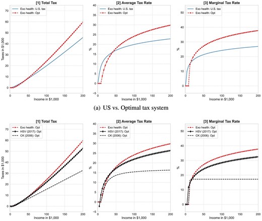
Optimal income taxes. Progressive income taxes of the benchmark case are based on Guner, Lopez-Daneri, and Ventura (2016),which uses the tax polynomial introduced in Benabou (2002). The optimal tax function consists of an income tax break of up to US|${\$}$|8,810, a scaling parameter of λ* = 1.277, and a tax progressivity parameter of τ* = 0.112. The black line with diamond markers is the optimal tax from Heathcote et al. (2017). The black dotted line is the optimal tax from Conesa and Krueger (2006), which is based on a model without health shocks and health insurance and a tax polynomial based on Gouveia and Strauss (1994) with three parameters.
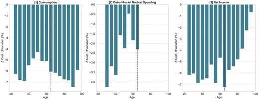
Change in the coefficient of variation by age group after introducing the optimal progressive income tax. We report the difference in the coefficient of variation of variable x by age group: CV(x-optimal)—CV(x-US benchmark), where x is either consumption, out-of-pocket medical spending, or net income.
In summary, the welfare gain for the lowest skill type can be large at up to |$1.8\%$| of lifetime consumption (compensating equivalent variation in consumption or CEV), whereas welfare losses can amount to |$2.6\%$| for the highest income types, as reported at the bottom of Table 4. Overall, we calculate a welfare gain of |$0.102\%$| at the aggregate level due to switching to the income tax system with optimal tax progressivity. The positive welfare outcome indicates that the welfare gains resulting from improvements in risk sharing and redistribution dominate the welfare losses from tax distortions and lower output.31
Suits Index.
In order to compare the progressivity levels across different income tax regimes, we follow Suits (1977) and compute a tax progressivity (Suits) index, which is a Gini coefficient for income tax contributions by income group as shown in Figure 7. The Suits index varies from +1 (most progressive, the entire tax burden falls on households of the highest income bracket), through 0 for a proportional tax, to —1 (most regressive, the entire tax burden falls on households of the lowest income bracket). The US income tax system in the benchmark model has a Suits index of 0.122, whereas the optimal US tax system is substantially more progressive with a Suits index of 0.218, which reduces income inequality significantly. The after-tax-income Gini coefficient decreases from 0.352 in the benchmark economy to 0.320 after the progressivity level is optimized.
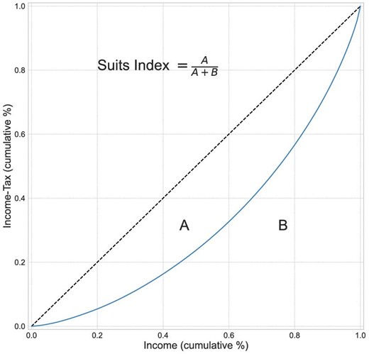
Lorenz curves and Suits index for the income taxes. The Tax Lorenz-type curve and Suits index measure the degree of disproportionality between pretax income and tax contributions by means of a relative concentration curve. The Suits index is essentially a Gini coefficient for tax contributions by income group. It varies from +1 (most progressive), where the entire tax burden is allocated to households of the highest income bracket, through 0 for a proportional tax, and to −1 (most regressive), where the entire tax burden is allocated to households of the lowest income bracket.
The Optimal Income Tax Polynomial.
Figure 5(a) compares the current US income taxes, average tax rates, and marginal tax rates—all plotted as functions of gross income—to their respective counterparts in the optimized income tax system. The optimal tax function consists of a progressivity parameter of |$\tau {}_{US}^{*}=0.113$| and a scaling parameter of |$\lambda _{US}^{*}=1.277$|. This level of progressivity is much higher than the US benchmark case with progressivity parameter τUS = 0.053. As already discussed earlier, the optimal tax system is characterized by a tax break for income earners below |${\$}$|8,810 followed by a steep increase in the marginal tax rate to |$20\%$| around income levels of |${\$}$|20,000 and a more moderate increase thereafter to marginal rates of over |$30\%$| for taxable income above |${\$}$|70,000 and around |$36\%$| for income above |${\$}$|150,000.
In panel [1] of Figure 5(a), we compare the tax burdens of the US benchmark economy to the economy with the optimal tax system. Under the optimal tax system very low income individuals pay almost zero taxes, whereas middle and high income individuals pay significantly more than under the current US income tax system. Panels [2] and [3] present the average and marginal tax rates, respectively. From panel [1], we see that individuals with income below |${\$}$|48,000 pay less in total taxes and benefit most from optimizing the progressivity level.32 Meanwhile, the tax burden shifts to individuals in the upper tail of the income distribution. For instance, individuals with taxable income exceeding |${\$}$|200,000 face average taxes that are roughly 8 percentage points higher than before the reform. Overall, the optimal income tax system is significantly more progressive than the current US system.
Connections to the Literature.
The optimal income tax system in our model is more progressive than the optimal progressivity found in previous studies. For comparison, we present our optimal tax progressivity results together with the optimal progressivity levels in Conesa and Krueger (2006) and Heathcote et al. (2017) in Figure 5(b). We emphasize that health risk and health insurance play a crucial role in explaining the differences in the observed optimal progressivity rates.
While our model has many similarities with the model in Conesa and Krueger (2006), there are some important differences. Their framework does not account for health states and the associated health spending risk explicitly. As a consequence, they also abstract from modeling health insurance contracts so that households rely on self-insurance via savings and adjusting labor supply as well as a minimum consumption floor that is maintained by the government. In their framework, labor productivity shocks are the only source of household heterogeneity. While this modeling assumption covers some of the health/income risk, it does not factor in health spending risk. In addition, as retirees are not exposed to income shocks anymore, their model abstracts from any risk associated with health that is not embedded in the average survival probability by age group. On the other hand, they use a less restrictive tax polynomial that is based on three parameters following Gouveia and Strauss (1994) as opposed to our two parameter tax polynomial. They find that the optimal level of tax progressivity is a proportional tax of |$17.2\%$| with a tax free threshold of about |${\$}$|9,400. Differently, in our model individuals are exposed to both income and health risks during their active work life and to health risk during retirement. Health risk affects the income process, triggers idiosyncratic health spending, and affects the survival probabilities. We also model the main institutional features of the US health insurance system. Our optimal tax function is more progressive and results in much higher marginal tax rates, especially at the high end of the income distribution as shown in panel [3] of Figure 5(a).33
Heathcote et al. (2017) use a similar functional form of progressive income taxes based on two parameters, but do not impose the non-negative tax restriction. However, their modeling approach is very different from ours as they do not explicitly model the US transfer programs such as Social Security, Medicare, Medicaid, and other means-tested transfers. They, in fact, combine many government spending programs into a public goods consumption (CG) component, which enters the household preferences. In addition, they use a perpetual youth model with skill investment and labor market shocks. Their perpetual youth model is therefore structurally very different from our large scale overlapping generations model with shocks to labor productivity and health status. They find that the optimal tax progressivity parameter is |$\tau _{HSV}^{*}=0.084$|, which is smaller than our optimal progressivity of |$\tau {}_{US}^{\ast }=0.113.$|34 Note that, Heathcote et al. (2017) do not explicitly model health expenditure shocks and the US health insurance system. They do, however, target consumption spending which includes some health expenditures. They also abstract from modeling precautionary saving and capital accumulation. It is perhaps not surprising that the optimal tax rate in our model is therefore much closer to their optimal tax rate than to Conesa and Krueger (2006).
The high marginal income tax rates found in our model are consistent with the recent income taxation literature (Diamond and Saez 2011; Badel, Huggett, and Luo 2020; Kindermann and Krueger 2022). In particular, Kindermann and Krueger (2022) show that very high marginal tax rates for the top one percent of income earners are primarily driven by the social insurance benefits that these high taxes imply. A similar mechanism is present in our framework, as households during their working age are simultaneously exposed to both, health and income risks, and households at retirement age are still exposed to health risk. Precautionary motives are relatively strong in our setting because health risk and out-of-pocket health expenditure shocks become more severe with as an individual gets older and especially after retirement, which is in line with the findings in De Nardi, French, and Jones (2010).
Thus, in the context of the US where the health insurance system is fragmented and only provides partial health insurance, the optimal income tax progressivity exhibits a higher level of progressivity in order to provide a sufficient level of redistribution and social insurance to unhealthy low income individuals who have limited access to health insurance. This result highlights that the health-related tax progressivity channel plays an important role in determining the optimal progressivity level of the US income tax system.
4.2. Isolating the Role of Health Spending Risk
In this section, we examine to what extent health spending risk contributes to the optimal progressivity level of the US income tax system. To do so, we take a step back and build a new quantitative model without health spending risk. We start from the benchmark model and remove the health spending risk. Removing medical spending will make the private health insurance system redundant so that premium payments for IHI and GHI are removed from the model. This simplified model does also not include the tax deductibility of premiums and catastrophic medical spending. This version of the model is therefore very similar to a standard Bewley–Aiyagari–Huggett incomplete markets model used in the macro and public finance literature such as Conesa and Krueger (2006).
Note, however, that this version of the model still allows for health dependent efficiency profiles |$e_{j}(\vartheta ,\epsilon _{j}^{n},h(\epsilon ^{h}))$| and survival probabilities πj(h(εh)). This means that the model still features idiosyncratic health states εh that follow a Markov process, which depends on age and the permanent income group so that conditional transition probabilities are elements of matrix Πh(j, ϑ). In this environment, individuals face permanent and transitory income shocks over the lifecycle as in the previous model. The progressive income tax system therefore provides a redistribution mechanism and social insurance against income and survival risk. Only the health-spending channel and as it relates to tax progressivity is removed in this setting. We also do not change any government policies so that taxes for Medicare and premium payments for Medicare are still in place. In order to match tax revenues from the original model, we scale up exogenous government consumption CG when we re-calibrate the model to match US data.35
We then again solve for the optimal tax progressivity level, which is the solution of the government maximization problem (23) in the absence of health expenditure risk. We summarize the new results in Table 5. We also display the associated optimal progressive tax schedule in Figures 8(a) and 8(b).
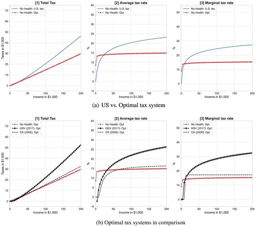
Optimal income taxes in model without health expenditure risk. For the benchmark US tax progressivity, we use estimates of the tax polynomial from Guner, Lopez-Daneri, and Ventura (2016). The blue solid line is the US tax case. The red line is the optimal tax progressivity in our model. It consists of no income tax break with a scaling parameter of λ* = 0.882 and a tax progressivity parameter of τ* = 0.007. The black line with diamond markers is the optimal tax from Heathcote et al. (2017). The black dotted line is the optimal tax from Conesa and Krueger (2006), which is based on a model without health shocks and health insurance and a tax polynomial based on Gouveia and Strauss (1994) with three parameters.
Model without health spending risk.
| (1) Bench. | (2) Optimized progressivity τ* | |
|---|---|---|
| Output (GDP) | 100 | 106.51 |
| Capital (K) | 100 | 110.86 |
| Non-medical consumption (C) | 100 | 106.80 |
| Labor participation rate | 66.86 | 65.27 |
| Weekly hours worked | 100 | 105.3 |
| Gini (net income) | 0.408 | 0.433 |
| Suits index (income tax) | 0.105 | 0.014 |
| Tax progressivity (τ) | 0.053 | 0.005 |
| Scaling parameter (λ) | 1.022 | 0.874 |
| Tax break threshold | |${\$}$|1,630 | |${\$}$|1 |
| Welfare (CEV): | 0 | +0.859 |
Notes: This table presents steady-state results from the model with income risk only. Health expenditure shocks are removed and health insurance is redundant from the model. This model shares a similar structure as the one in Conesa and Krueger (2006). Column (1) shows steady-state results of the new benchmark economy without health spending risk. Column (2) shows steady-state results for an identical economy with a welfare maximizing (optimal) progressive income tax system. Numbers in rows marked with the % symbol are either fractions in percent or tax rates in percent. The other rows are normalized with values of the benchmark case. Each column presents steady-state results. CEV values are reported as percentage changes in terms of lifetime consumption of a newborn individual with respect to consumption levels in the benchmark.
The new optimal income tax function changes significantly once health spending risk is removed from the model. The optimal tax function now removes the income tax deductibility and imposes a tax progressivity of |$\tau _{\text{noH-risk}}^{*}=0.005$|, which is very close to a flat marginal tax rate. The scaling parameter is |$\lambda _{\text{noH-risk}}^{*}=0.874$|. As shown in Figure 8(a), the entire tax function shifts downward and flattens out. The marginal tax rates are significantly lower for all households. The Suits index for the optimal tax system decreases to 0.014, which is much lower than the Suits index of 0.218 for the optimal tax in the model with health spending risk.
The main conclusion is that the optimal income tax system is much less progressive in the model without health risk. The mechanism behind this result is straightforward. In the model with health expenditure risk, the progressive income tax system has two social insurance roles: (i) redistributing income across different earnings ability groups and insuring against income risk, and (ii) supplementing the social health insurance function of the fragmented US health insurance system that fails to provide health insurance to some individuals. The latter mechanism exists only in models with health spending risk and therefore leads to more progressive income taxation. This result implies that most of the benefits of highly progressive taxes stem from social health insurance rather than income redistribution and consumption floor insurance. Furthermore, the precautionary savings motive is much stronger in a model with exogenous health spending risk than in a model where health spending is implicitly part of consumption that a household can smooth over the lifecycle. With a strong precautionary savings channel in place, the savings distortions caused by higher tax progressivity will be muted and a social planner is going to be able to impose a more progressive tax system without triggering massive decreases in capital stock and GDP.
In order to clarify this result, we compare our optimal tax system without health spending risk to the optimal tax system in Conesa and Krueger (2006), which is also a model without explicit health risk. As shown in panel [3] of Figure 8(b), the optimal income tax system looks very similar to theirs and is essentially a flat tax rate of |$15\%$|. This is only slightly lower than the optimal flat tax rate of |$17.2\%$| in their paper.36
Overall, we reach a similar conclusion in that the optimal tax system in a model without health expenditure risk exhibits a lower level of progressivity than the existing US income tax scheme. This finding emphasizes the quantitative importance of the social health insurance role of progressive income taxes in a model where individuals are exposed to health spending risk.
4.3. Interactions between Health Insurance and Optimal Tax Progressivity
In a model with health risk, a health insurance system can be devised to reduce or possibly completely remove health expenditure risk. In this section, we examine the effect of alternative health insurance designs on the optimal degree of income tax progressivity. We specifically consider two alternative health insurance arrangements: (i) no health insurance, and (ii) universal public health insurance (hereafter, UPHI).
4.3.1. No Health Insurance
We begin with the no health insurance case, where all forms of private and public health insurance such as IHI, GHI, Medicare, and Medicaid and associated taxes are removed from the model. In this setting, individuals exclusively rely on their own income from savings and labor supply to cover health expenditures (self-insurance). The out-of-pocket health expenditure is therefore given by m(j, ϑ, εh). The model again inherits the structural parameter values for preferences, technologies, labor productivity profiles, and health shocks from the US calibration. All fiscal policies including social security, consumption floor insurance, general government consumption, and taxes are kept at US levels. However, the entire health insurance system, public and private insurance, is eliminated.
We then search for the optimal income tax progressivity rate |$\tau _{noHI}^{*}$| that solves the government maximization problem (23) with no health insurance. We report the macroeconomic and welfare effects in column (3) of Table 6. For comparison, we also repeat the US benchmark steady-state values in column (1) and the steady-state values for the US benchmark model with optimal income taxes in column (2).
Alternative health insurance systems in model with health spending risk.
| Optimized tax progressivity τ* | ||||||||
|---|---|---|---|---|---|---|---|---|
| (1) | (2) | (3) | (4) | (5) | (6) | (7) | (8) | |
| Benchmark | US-HI | No HI | ρUPHI | |||||
| |$\overset{\text{Full}}{\overbrace{0}}$| | |$\overset{\text{Partial}}{\overbrace{0.3}}$| | |$\overset{\text{Partial}}{\overbrace{0.5}}$| | |$\overset{\text{Optimal}}{\overbrace{0.55}}$| | |$\overset{\text{Null}}{\overbrace{1}}$| | ||||
| Output (GDP) | 100 | 93.36 | 106.61 | 85.86 | 95.12 | 93.88 | 98.18 | 107.24 |
| Capital (K) | 100 | 90.77 | 113.34 | 74.72 | 90.53 | 91.54 | 98.09 | 115.16 |
| Non-medical consumption (C) | 100 | 93.25 | 104.75 | 87.97 | 95.74 | 92.88 | 96.86 | 104.97 |
| Labor participation rate | 67.14 | 69.21 | 73.64 | 62.07 | 67.18 | 71.70 | 72.29 | 73.06 |
| Weekly hours worked | 100 | 93.92 | 97.42 | 98.58 | 98.18 | 92.33 | 94.09 | 98.05 |
| Workers insured (%) | 80.40 | 81.58 | 0 | 100 | 100 | 100 | 100 | 100 |
| Retirees insured (%) | 100 | 100 | 0 | 100 | 100 | 100 | 100 | 100 |
| Interest rate |$(r\text{ in $\%$})$| | 5.9 | 6.16 | 5.36 | 7.30 | 5.39 | 6.13 | 5.75 | 5.27 |
| Wage rate (w) | 100.00 | 98.48 | 103.34 | 92.40 | 97.22 | 98.70 | 99.98 | 103.91 |
| Gini (income) | 0.353 | 0.320 | 0.292 | 0.413 | 0.359 | 0.300 | 0.311 | 0.291 |
| Gini (health expenditure) | 0.548 | 0.543 | 0.560 | 0.960 | 0.547 | 0.553 | 0.554 | 0.560 |
| Suits index (income tax) | 0.122 | 0.218 | 0.369 | 0.003 | 0.070 | 0.225 | 0.224 | 0.415 |
| Tax progressivity (τ) | 0.053 | 0.113 | 0.155 | 0.003 | 0.039 | 0.102 | 0.110 | 0.155 |
| Scaling parameter (λ) | 1.017 | 1.277 | 1.603 | 0.710 | 0.900 | 1.317 | 1.267 | 1.646 |
| Tax break threshold | |${\$}$|1,402 | |${\$}$|8,810 | |${\$}$|21,022 | |${\$}$|1 | |${\$}$|201 | |${\$}$|9,210 | |${\$}$|8,810 | |${\$}$|25,226 |
| Welfare (CEV in %): | 0 | +0.102 | −4.651 | −7.411 | −2.047 | −0.936 | −0.586 | −5.051 |
| • Income group 1 (sick) | 0 | +1.815 | −0.631 | ( − ) | ( − ) | ( + ) | ( + ) | ( − ) |
| • Income group 2 (sick) | 0 | +0.724 | −7.390 | ( − ) | ( − ) | ( − ) | ( − ) | ( − ) |
| • Income group 2 (healthy) | 0 | +1.159 | −6.950 | ( − ) | ( − ) | ( + ) | ( + ) | ( − ) |
| • Income group 3 (healthy) | 0 | −2.584 | −3.814 | ( − ) | ( − ) | ( − ) | ( − ) | ( − ) |
Notes: Column (1) shows steady-state results of the benchmark economy based on the US income tax and health insurance system. Column (2) shows steady-state results for optimal income taxes with the US health insurance system. Column (3) shows steady-state results for optimal income taxes without any health insurance in place. Columns (4)–(8) show results with a UPHI system with coinsurance rate |$\rho ^{\textit {UPHI}}$|ranging from 0 (full insurance) to 1 (no insurance). All UPHI systems are financed by the progressive income tax system. The difference between column (3) No health insurance and column (8) UPHI with 100% coinsurance is that in the UPHI experiments the Medicare payroll tax is left in place whereas in the No-health-insurance version of the model all elements of insurance, public or private, are removed from the model. Data in rows marked with the % symbol are either fractions in percent or tax rates in percent. All other rows are normalized with values of the benchmark case. CEV values are reported as percentage changes in terms of lifetime consumption of a newborn.
Without any health insurance, individuals are fully exposed to health expenditure shocks, especially at the end of the lifecycle where health expenditure shocks tend to be large and have a higher probability of occurring. Individuals therefore work longer hours and save more in order to self-insure against the health expenditure shocks. These precautionary motives raise capital accumulation and labor supply at the aggregate level, which subsequently leads to a large expansion of the economy. As reported in column (3), output and capital stock increase by |$6.6\%$| and |$13\%$|, respectively, compared to the benchmark economy. In addition, consumption levels are |$4.75\%$| higher.
The optimal tax function for the no insurance case implies a tax free income threshold of |${\$}$|21,000, a scaling parameter of |$\lambda _{noHI}^{*}=1.603,$| and a tax progressivity parameter of |$\tau _{noHI}^{*}=0.155.$| The optimal total and average tax schedules shift downward compared to the optimal tax case with the US health insurance system in place. This is shown in panels [1] and [2] in Figure 9. The zero tax income threshold at |${\$}$|21,000 is much higher than the threshold of |${\$}$|8,800 under the optimal tax regime with the US health insurance system in place. The marginal income tax rates are also higher for income above |${\$}$|50,000 as shown in panel [3] of Figure 9. The rates imposed on incomes above |${\$}$|150,000 are around |$38\%$|. These increases are mainly due to a much larger demand for tax revenue from the top end of the income distribution in order to balance the government budget after further cutting taxes for individuals at the lower end of the income distribution. The Suits index increases to 0.369, which is higher than 0.122 in the benchmark and also higher than 0.218 from the optimal tax case with the US health insurance institutions in place (compare column (2) in Table 6).
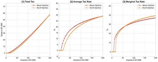
No health insurance and optimal income tax progressivity in health risk model. The optimal tax function consists of an income tax break of up to US|${\$}$|21,022, a scaling parameter of λ* = 1.601, and a tax progressivity parameter of τ* = 0.155.
The health insurance system provides an important mechanism for sharing health risk by redistributing income to relatively sicker households. Turning off the health insurance system strengthens the redistribution and social insurance function of the progressive income tax system. As a result, income tax progressivity increases in the optimum compared to environments with some form of health insurance in place.
4.3.2. Universal Public Health Insurance
The current US health insurance system relies heavily on private, employer sponsored, health insurance to cover the working age population, while public health insurance predominantly focuses on insuring the retired (through Medicare) and individuals with low income (through Medicaid). As a result of this fragmented approach, a significant share of the population does not have health insurance. We therefore analyze how removing this fragmentation by extending Medicare to all individuals, that is, UPHI, affects the optimal income tax progressivity level.
When we introduce the UPHI system, we need to set the coinsurance rate |$\rho ^{\textit {UPHI}}\in \left[0,1\right].$| The lower the level of the coinsurance rate is set, the more insurance is provided against health expenditure shocks. A coinsurance of zero provides full insurance, while a coinsurance rate of one (or 100%) would not provide any insurance.37
When we solve the various UPHI versions of the model we keep social security, the consumption floor insurance, government consumption, and all taxes at the benchmark levels, while eliminating all private health insurance (GHI and IHI) programs. We do not recalibrate the UPHI models. We then again solve for the optimal level of tax progressivity of each version of the UPHI model (distinguished only by the UPHI coinsurance rate) and report the results in columns (4)–(8) of Table 6. We first discuss the results of a UPHI system with the current Medicare coinsurance rate of 30%. The results for this experiment are shown in column (5) of Table 6.
Aggregate effects. The fiscal distortions caused by income tax increases that are needed to finance the UPHI program are significant. The payments through the UPHI system as well as the higher taxes needed to finance it both distort the incentives to save and work. Weekly hours worked decrease by almost |$2\%$|. Similarly, the capital stock decreases by almost |$10\%$|. These distortions lead to significant efficiency losses and result in a |$5\%$| decrease of GDP. As the economy shrinks, households have less income which leads to welfare losses. On the other hand, the UPHI system improves health risk sharing which can improve welfare. The overall welfare loss of −2.047 of compensating lifetime consumption is the result of the negative incentive effects dominating the positive insurance and redistribution effects. We do, however, observe that the welfare losses are smaller for low income groups at |$-0.25\%$| of CEV as opposed to the much larger losses of |$-3.33\%$| of CEV of the high income group.
The optimal income tax polynomial. UPHI provides (social) health insurance for all types of individuals in the economy, especially members of the poor working class who are not covered by the US healthcare system. In this setting, the demand for social insurance provided through the progressive income tax system decreases and therefore the optimal degree of progressivity decreases as well.
The welfare maximizing progressivity level of the UPHI system with a 30% coinsurance rate exhibits a much lower tax progressivity parameter of |$\tau _{\textit {UPHI}}^{*}=0.039$| than the optimal progressivity under the US healthcare system |$\tau _{US}^{*}=0.113$| (see column (2) of Table 6). The new optimal income tax schedule shifts to the left in Figure 10 and the tax free income threshold decreases significantly to |${\$}$|200, which is much smaller than threshold of |${\$}$|8,810 in the model with the US health insurance system in place. The marginal income tax rates are larger on income below |${\$}$|60,000 but lower for income above |${\$}$|60,000. The rates imposed on incomes above |${\$}$|150,000 are lower at |$32\%$|, compared to around |$35\%$| under the optimal tax system in the benchmark US model. The Suits index of the optimal tax system in this environment decreases to 0.070 and indicates that the tax system is less progressive than the optimal tax system in the model with the US healthcare system.
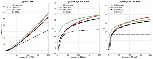
Optimal income tax progressivity and UPHI in health risk model. Optimal progressivity levels are calculated for (i) US health insurance (in red), and (ii) UPHI with 30% coinsurance (partial insurance similar to Medicare). The black line with diamond markers is the optimal tax from Heathcote et al. (2017). The black dotted line is the optimal tax from Conesa and Krueger (2006), which is based on a model without health shocks and health insurance and a tax polynomial based on Gouveia and Strauss (1994) with three parameters.
It is important to note that the new optimal income tax function moves toward the optimal ones in Conesa and Krueger (2006) and Heathcote et al. (2017). The mechanism behind this change is as follows. The introduction of UPHI with a coinsurance rate of |$30\%$| reduces the individual exposure to health shocks by |$70\%$|. This makes the model’s incentive structure more similar to previous studies that abstract from health expenditure risk and health insurance. In addition, this expansion of public (social) health insurance significantly reduces the demand for additional social health insurance through the progressive income tax system.
Thus, this quantitative finding confirms that the social insurance role of the progressive income tax system interacts with the social insurance role of public health insurance. The optimal progressivity level of an income tax system therefore depends critically on the design (or generosity) of the health insurance system.
The effect of coinsurance rates in the UPHI system. As already mentioned in the introduction to this section, in a UPHI system, the intensity of a household’s exposure to health expenditure shocks is determined by the coinsurance rate. If the coinsurance rate is set at a higher level, then individuals pay for a larger share of their total health expenditure out-of-pocket and must therefore either reduce their consumption or increase their cash-on-hand by either working more or saving less to account for sudden health related expenditures.38 This higher exposure to health spending risk decreases welfare of risk averse households. On the government side, a high coinsurance rate implies a smaller (less generous) public health insurance program that requires less tax revenue and therefore creates fewer tax distortions. This results in efficiency gains and higher income, which increases welfare.
Taken together, implementing UPHI with a specific coinsurance rate trades off negative incentive effects with positive insurance/redistribution effects. The sum of these will determine the overall effect on household welfare. Since the government has aggregate household welfare in mind when solving for the optimal level of income tax progressivity, the UPHI coinsurance rate will have a direct effect on the optimal degree of income tax progressivity as the need for more insurance/redistribution through the progressive tax system is strongly determined by how much risk the UPHI system already removes. In order to measure the magnitude of this effect, we implement the UPHI system with a number of different coinsurance rates in the range from 0% (full insurance) to 100% (no insurance). We then solve for the optimal tax progressivity level and report the results in Table 6 and Figure 11.
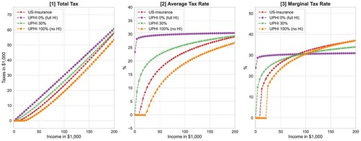
Generosity of UPHI and optimal tax progressivity in health risk model. For the benchmark US tax progressivity (red line with stars), we use estimates of the tax polynomial from Guner, Lopez-Daneri, and Ventura (2016). For the UPHI cases, the coinsurance rates are set to 0% (full insurance), 30% (partial insurance) and 100% (no insurance). If the UPHI is the most generous—UPHI with 0 coinsurance—then the optimal income tax system is the least progressive. If the UPHI is the least generous—UPHI with 100% coinsurance—then the optimal income tax system is the most progressive.
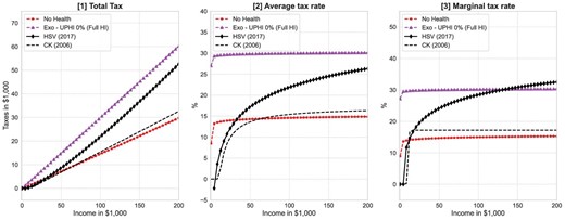
No health risk model versus health risk model with full insurance. In the No health risk model, we remove the exogenous health spending process and all private insurance programs. The UPHI 0% model is a model with exogenous health spending but a UPHI system with no coinsurance (full insurance). The black line with diamond markers is the optimal tax from Heathcote et al. (2017). The black dotted line is the optimal tax from Conesa and Krueger (2006), which is based on a model without health shocks and health insurance and a tax polynomial based on Gouveia and Strauss (1994) with three parameters.
A more generous UPHI system with lower coinsurance rates provides more (social) health insurance for low income and sick individuals and therefore reduces the need for high marginal taxes on high income earners to achieve welfare improving re-distribution. For the most generous UPHI case, |$\rho ^{\textit {UPHI}}=0$|, individuals pay no healthcare cost out of pocket, that is, o(mj) = 0. In this setting, even though individuals still face health risk via health dependent survival probabilities and health dependent labor market efficiency profiles, their exposure to health expenditure shocks is removed by the health insurance system. We find that in this case, the optimal income tax system is characterized by a flat tax (as the tax progressivity parameter approaches zero |$\tau _{\textit {UPHI}}^{*}=0.003$|), a scaling parameter of |$\lambda _{\textit {UPHI}}^{*}=0.71,$| and a complete removal of income tax deductibility. (see column (4) of Table 6). This outcome is very close to the optimal tax in our model with no health risk (compare Figure 12) or the model in Conesa and Krueger (2006). However, the tax burden increases dramatically as the government has to finance fairly large health insurance program. This generates large output losses so that overall welfare decreases.
For a less generous UPHI case, that is, |$\rho ^{\textit {UPHI}}=0.5$|, the optimal tax system becomes more progressive with a tax progressivity parameter value of |$\tau _{\textit {UPHI}}^{*}=0.102$|, which looks more similar to the one reported Heathcote et al. (2017). Finally, when the UPHI coinsurance rate is set to |$100\%$|, that is, |$\rho ^{\textit {UPHI}}=1,$| individuals pay for all health expenditures out-of-pocket. Under this null UPHI system, individuals exclusively rely on self-insurance via savings and labor. The optimal income tax system becomes a lot more progressive with a tax progressivity parameter of |$\tau _{\textit {UPHI}}^{*}=0.155$| (see the column (8) in Table 6).39
In conclusion, we demonstrate an inverse relationship between the generosity of the UPHI system and the optimal tax progressivity as shown in the entries for the tax progressivity parameter τ across columns (4)–(8) in Table 6. As the exposure to health expenditure shocks is reduced or removed by making public health insurance more generous, the need to redistribute or insure through the income tax system decreases and the optimal tax system becomes less progressive. This result confirms that the optimal design of a progressive income tax system is strongly influenced by the concurrent design of the health insurance system in models with health expenditure risk.
5. Robustness Checks
In this section, we investigate whether the mechanism discovered in the previous section prevails under different modeling and calibration assumptions, including alternative values of preference parameters and health in utility as a preference shifter.
5.1. Preferences
In this section, we assess the robustness of our results with respect to changes in values of preference parameters. We choose alternative parameter values for the preference weight on consumption η (0.27 and 0.28) and the risk aversion parameter σ (2.5 and 3.5 ). These parameters determine the level of risk aversion as well as the labor supply elasticity. Note that, we only consider one-dimensional changes in the model. We recalibrate the model after each change by adjusting the discount factor β so that the model exhibits the benchmark capital output ratio of 3 again. We then solve for the optimal level of income tax progressivity as before and present the results in Table 7.
US HI system and optimal progressive taxation with alternate preference parameters.
| (1) | (2) | (3) | (4) | (5) | |
|---|---|---|---|---|---|
| Benchmark | $\begin{array}{l}\eta =0.265\\
\sigma =3.0 \end{array}$ | $\begin{array}{l}\eta =0.28\\
\sigma =3.0 \end{array}$ | $\begin{array}{l}\eta =0.272\\
\sigma =2.5 \end{array}$ | $\begin{array}{l}\eta =0.272\\
\sigma =3.5 \end{array}$ | |
| Output (GDP) | 93.36 | 94.38 | 95.73 | 95.46 | 92.98 |
| Capital (K) | 90.77 | 92.03 | 93.98 | 93.17 | 90.61 |
| Non-medical consumption (C) | 93.25 | 94.39 | 95.76 | 95.49 | 92.079 |
| Frisch labor elasticity range | 1.19–1.51 | 1.18–1.50 | 1.20–1.53 | 1.30–1.66 | 1.11–1.41 |
| Suits index (income tax) | 0.218 | 0.207 | 0.192 | 0.187 | 0.223 |
| Optimal Tax Progressivity (τ*) | 0.113 | 0.105 | 0.097 | 0.092 | 0.117 |
| Scaling parameter (λ) | 1.017 | 1.239 | 1.200 | 1.179 | 1.297 |
| Tax break threshold | |${\$}$|8,810 | |${\$}$|7,809 | |${\$}$|6,808 | |${\$}$|6,007 | |${\$}$|9,410 |
| Welfare (CEV in %): | +0.102 | +0.257 | +0.569 | +0.106 | +0.147 |
Notes: The US health insurance system is kept unchanged as in the benchmark economy. Each column shows steady-state results for an identical economy with a welfare maximizing (optimal) progressive income tax system. Numbers in rows marked with the % symbol are either fractions in percent or tax rates in percent. The other rows are normalized with values of the benchmark case. CEV values are reported as percentage changes in terms of lifetime consumption of a newborn individual with respect to consumption levels in the benchmark model.
In the model with the US health insurance, system variations in the preference parameter η have only small effects on the Frisch labor supply elasticities and the progressivity parameter τ as shown in Table 7. Qualitatively the results are identical and quantitatively the optimal progressive level ranges from 0.092 to 0.117. They all exhibit a much higher degree of progressivity than the benchmark progressivity level of 0.053.
Similarly, making individuals less risk averse by lowering parameter σ from 3.0 to 2.5 also does not change the main conclusion qualitatively. In an economy with lower values of risk aversion (σ = 2.5), the optimal tax progressivity is τ* = 0.092, and a scaling parameter of λ* = 1.179, which implies a tax free income threshold of |${\$}$|6,000. That is, the optimal income tax system is again more progressive than the US tax system. Our result is also robust to higher values of risk aversion (σ = 3.5). In this case, the optimal level of tax progressivity is slightly higher at 0.117. Overall, we consistently find that the optimal income tax system is more progressive than the benchmark system under alternative values of preference parameters.
When we introduce a more inclusive health insurance system, such as Medicare-for-all (UPHI with a |$30\%$| coinsurance rate), the optimal level of tax progressivity is much lower, ranging between 0.041and0.071 for all variations of parameter values of η and σ as shown in Table 8. We thus conclude that overall our findings are robust with respect to the considered range of risk aversion and consumption/leisure preference parameter values.
Optimal progressive taxation in UPHI (ρUPHI = 0.3) model with alternate preference parameters.
| (1) | (2) | (3) | (4) | (5) | |
|---|---|---|---|---|---|
| Benchmark | $\begin{array}{l}\eta =0.265\\
\sigma =3.0 \end{array}$ | $\begin{array}{l}\eta =0.28\\
\sigma =3.0 \end{array}$ | $\begin{array}{l}\eta =0.272\\
\sigma =2.5 \end{array}$ | $\begin{array}{l}\eta =0.272\\
\sigma =3.5 \end{array}$ | |
| Output (GDP) | 95.12 | 95.20 | 91.55 | 93.56 | 90.94 |
| Capital (K) | 90.53 | 90.84 | 85.81 | 88.64 | 84.99 |
| Non-medical consumption (C) | 95.74 | 95.71 | 91.93 | 94.01 | 91.25 |
| Suits index (income tax) | 0.070 | 0.072 | 0.107 | 0.094 | 0.107 |
| Optimal tax progressivity (τ*) | 0.039 | 0.041 | 0.071 | 0.057 | 0.071 |
| Scaling parameter (λ) | 0.900 | 0.904 | 1.015 | 0.964 | 1.016 |
| Tax break threshold | |${\$}$|201 | |${\$}$|201 | |${\$}$|1,402 | |${\$}$|602 | |${\$}$|1,402 |
| Welfare (CEV in %): | −2.074 | −2.921 | −2.081 | −2.022 | −2.411 |
Notes: The US health insurance system is replaced by a universal public health insurance (UPHI) system that has a coinsurance rate of 30%. Each column shows steady-state results with a welfare maximizing (optimal) progressive income tax system. Numbers in rows marked with the % symbol are either fractions in percent or tax rates in percent. The other rows are normalized with values of the benchmark case. CEV values are reported as percentage changes in terms of lifetime consumption of a newborn individual with respect to consumption levels in the benchmark.
5.2. Health-in-Utility (HIU) Preferences
We next model health status as a consumption good, which introduces a utility-health channel into the model. In this setting, there are now two channels through which the exogenous health states affect household welfare: (i) via the household budget constraint (as in our benchmark model), and (ii) via a preference shifter that depends on health status h, which is a function of the exogenous health states εh. We follow the approach in De Nardi, French, and Jones (2010) and assume that each period the individual’s utility depends on consumption, leisure, and health status, h, according to
where θ(h(εh)) is preference shifter and health state h(εh) is restricted to either either good/healthy (h = 1) or bad/sick (h = 0) based on health status εh. The assignment into healthy and sick state follows again the definition in expression 19. Following De Nardi, French, and Jones (2010), we specify the preference shifter as θ(h) = 1 + θh × h and set parameter θh = −0.36. Given our parameterization, this results in uc > 0, uh > 0 and uc,h < 0. In other words, if an individual moves from healthy (h = 1) to sick (h = 0), her consumption spending c is going to increase.40 We keep all other components of the benchmark model unchanged when we re-calibrate the benchmark model to match the US data.
We solve again for optimal income tax progressivity and summarize the results in Table 9. From columns (1)–(2), we see that the optimal progressivity level in the model based on the US health insurance system is not affected by adding a health shifter into the utility function. The progressivity level is essentially identical across the two model versions. As already discussed, the optimal tax system is more progressive than the current US system.
HIU and optimal tax progressivity in health risk model.
| US-HI | UPHI | UPHI | UPHI | |||||
|---|---|---|---|---|---|---|---|---|
| |$\overset{\text{Full}}{\overbrace{\rho ^{\textit {UPHI}}=0.0}}$| | |$\overset{\text{Partial}}{\overbrace{\rho ^{\textit {UPHI}}=0.30}}$| | |$\overset{\text{Null}}{\overbrace{\rho ^{\textit {UPHI}}=1.0}}$| | ||||||
| (1) | (2) | (3) | (4) | (5) | (6) | (7) | (8) | |
| Benchmark | HIU | Benchmark | HIU | Benchmark | HIU | Benchmark | HIU | |
| Output (GDP) | 93.36 | 93.45 | 85.86 | 85.25 | 95.12 | 91.66 | 107.24 | 108.24 |
| Capital (K) | 90.77 | 90.76 | 74.72 | 73.30 | 90.54 | 85.82 | 115.16 | 117.45 |
| Non-medical consumption (C) | 93.25 | 93.42 | 87.97 | 88.28 | 95.74 | 92.56 | 104.97 | 105.85 |
| Suits index (income tax) | 0.218 | 0.220 | 0.004 | 0.004 | 0.070 | 0.109 | 0.415 | 0.464 |
| Optimal tax progressivity (τ*) | 0.113 | 0.113 | 0.003 | 0.004 | 0.039 | 0.071 | 0.155 | 0.178 |
| Scaling parameter (λ) | 1.277 | 1.277 | 0.710 | 0.713 | 0.900 | 1.015 | 1.646 | 1.821 |
| Tax break threshold | |${\$}$|8,810 | |${\$}$|8,810 | |${\$}$|1 | |${\$}$|0 | |${\$}$|201 | |${\$}$|1,402 | |${\$}$|25,226 | |${\$}$|28,830 |
| Welfare (CEV in %): | +0.102 | +0.137 | −7.411 | −6.588 | −1.837 | −1.581 | −5.051 | −6.272 |
Notes: Similarly to De Nardi, French, and Jones (2010), health acts as a preference shifter in the HIU (health-in-utiliity) model. Columns (1) and (2) show steady-state results for a welfare maximizing progressive tax system with the US health insurance system in place. Column (1) is the benchmark model and column (2) shows the HIU version of the model. Columns (3) and (4) compare the optimal tax progressivity results for the benchmark model and the HIU model with a UPHI system that fully insures all health expenditure shocks, that is, the coinsurance rate is zero. Columns (5) and (6) compare the optimal progressivity outcome for a model with Medicare-for-all in place, that is, a UPHI with a coinsurance rate of 30%. Finally, columns (6) and (7) compare the optimal progressivity outcome for a model without health insurance, that is, a UPHI with a coinsurance rate of 100%. All private insurance arrangements are turned-off in the UPHI models. GDP, capital, non-medical consumption, and welfare are normalized using either the benchmark model with health risk or the recalibrated benchmark of the HIU model. Each column presents steady-state results. CEV values are reported as percentage changes in terms of lifetime consumption of a newborn individual with respect to consumption levels in the benchmark.
In the model with full insurance (a UPHI coinsurance rate of zero), we also find very little effect of the health-utility channel. In both cases, benchmark and HIU, the optimal progressive income tax is essentially a flat tax. Once we allow for more health expenditure risk by increasing the coinsurance rate of the UPHI system, say to 30%, we begin to see small effects of the health-utility channel on the level of optimal tax progressivity. Column (5) shows that without the health-utility channel the optimal progressivity is τ* = 0.039 and the tax free income threshold is |${\$}$|200, whereas column (6) shows that with an active health-utility channel the optimal tax progressivity is higher |$\tau _{\textit {HIU}}^{*}=0.071$| and the tax free income threshold is |${\$}$|1,400. We find a similar discrepancy between the model with and without the health-utility channel when we essentially remove health insurance by setting the coinsurance rate of UPHI to 100%. Again, the presence of the HIU channel increases the progressivity from τ* = 0.155 to |$\tau _{\textit {HIU}}^{*}=0.178$| and the zero tax thresholds from |${\$}$|25,000 to |${\$}$|29,000. This shows that the health-utility channel adds risk to the system that begins to affect the optimal progressivity level, if the health insurance system is not removing the health spending risk sufficiently.
5.3. Additional Robustness Exercises
We next consider the following three alternative specifications in the benchmark model with the US health insurance system: (i) the addition of a corporate income tax and explicit state and local income taxes as flat taxes similar to Guner, Lopez-Daneri, and Ventura (2016); (ii) sensitivity analysis with respect to parameters determining the labor productivity process; and (iii) a higher minimum consumption floor. We recalibrate the benchmark for each specification change and search for the optimal level of tax progressivity as in the earlier sections. We summarize our main results below and in Table 10.
Optimal progressive taxation with alternative modeling assumptions.
| (1) | (2) | (3) | (4) | (5) | |
|---|---|---|---|---|---|
| Benchmark | $\begin{array}{r}\tau ^{I}=0.05\\
\tau ^{K}=0.074 \end{array}$ | $\begin{array}{r}\rho =0.95\\
\\
\end{array}$ | $\begin{array}{r}\sigma _{\varepsilon }^{2}=0.02\\
\\
\end{array}$ | $\begin{array}{r}c_{min}=\$4,000\\
\\
\end{array}$ | |
| A. US health insurance system | |||||
| + Optimal tax progressivity (τ*) | 0.113 | 0.122 | 0.072 | 0.150 | 0.117 |
| + Scaling parameter (λ) | 1.277 | 1.453 | 1.101 | 1.492 | 1.863 |
| + Tax break threshold | |${\$}$|8,810 | |${\$}$|6,608 | |${\$}$|1,600 | |${\$}$|1,630 | |${\$}$|1,200 |
| + Suits index (income tax) | 0.218 | 0.196 | 0.157 | 0.295 | 0.206 |
| B. UPHI system with |$\rho ^{\textit {UPHI}}=0.3$| | |||||
| + Optimal tax progressivity (τ*) | 0.039 | 0.053 | 0.04 | 0.071 | 0.109 |
| + Scaling parameter (λ) | 0.900 | 1.020 | 0.893 | 1.006 | 1.168 |
| + Tax break threshold | |${\$}$|201 | |${\$}$|1,600 | |${\$}$|200 | |${\$}$|1,200 | |${\$}$|4,200 |
| + Suits index (income tax) | 0.070 | 0.112 | 0.064 | 0.102 | 1.141 |
| C. UPHI system with |$\rho ^{\textit {UPHI}}=0.0$| | |||||
| + Optimal Tax Progressivity (τ*) | 0.003 | 0.006 | 0.023 | 0.008 | 0.066 |
| + Scaling parameter (λ) | 0.710 | 0.785 | 0.770 | 0.726 | 0.914 |
| + Tax break threshold | |${\$}$|1 | |${\$}$|0 | |${\$}$|0 | |${\$}$|0 | |${\$}$|400 |
| + Suits index (income tax) | 0.003 | 0.008 | 0.022 | 0.007 | 0.060 |
| D. UPHI system with |$\rho ^{\textit {UPHI}}=1.0$| | |||||
| + Optimal tax progressivity (τ*) | 0.155 | 0.112 | 0.117 | 0.142 | 0.133 |
| + Scaling parameter (λ) | 1.646 | 1.493 | 1.406 | 1.553 | 1.460 |
| + Tax break threshold | |${\$}$|25,226 | |${\$}$|33.837 | |${\$}$|18,820 | |${\$}$|22,420 | |${\$}$|17,418 |
| + Suits index (income tax) | 0.415 | 0.509 | 0.341 | 0.382 | 0.310 |
Notes: Column (1) reports steady-state results for the benchmark economies with a welfare maximizing (optimal) progressive income tax system. Next four columns report steady-state results under alternative assumptions. There are four experiments in consideration: (2) State and local income taxes as well as a linear tax on capital, (3) Less persistent labor shock process with ρ = 0.95 from ρ = 0.977 in the benchmark, (4) Larger variance of labor shock disturbance |$\sigma _{\varepsilon }^{2}=0.02$| from |$\sigma _{\varepsilon }^{2}=0.0141$| in the benchmark, and (5) Higher minimum consumption floor |$c_{\textit {min}}=\$4,000$| from |$c_{\textit {min}}=\$2,\!500$| in the benchmark. All models under alternative assumptions are re-calibrated to match the same set of moments as the benchmark model before we search for the optimal tax progressivity τ*.
Corporate Income Tax and State and Local Income Taxes.
We consider a modification to the income tax system by introducing an additional flat tax on income τI = 0.05 to approximate state and local income taxes as well as an additional capital income tax τK = 0.074 to approximate the corporate income. Our approach is similar to the one Guner, Lopez-Daneri, and Ventura (2016). We find that the changes to the income tax system result in small changes in the quantitative results. For example, the optimal tax progressivity has a value of τ* = 0.122 as opposed to τ* = 0.113 in our base specification without local and explicit corporate income taxes.
Changes to the Labor Productivity Process.
The labor productivity shock is modeled as an auto-regressive process as shown in expression 20 with persistence parameter ρ and a white noise disturbance |$\varepsilon \sim N\left(0,\sigma _{\varepsilon }^{2}\right)$|. In our benchmark calibration, we use ρ = 0.977 and |$\sigma _{\varepsilon }^{2}=0.0141$| based on estimates in French (2005). In our model, we adjust the parameter values for the 5 year time period. However, we do no account for gender differences as we abstract from modeling family structure. In our robustness check, we therefore consider cases in which we allow for small changes in the values for the persistence parameter ρ = 0.95 and the variance of the innovation |$\sigma _{\varepsilon }^{2}=0.02$|. We find that these changes do not change our conclusions.
Changes to the Minimum Consumption Floor.
We next increase the minimum consumption floor to |$c_{\textit {min}}=\$4,000$|. We rerun the optimization experiment and find that a higher minimum consumption floor does not alter our main results.
Endogenous Health Expenditure.
We also consider an endogenous health model in which health evolves endogenously over the lifecycle similar to the concept of health capital introduced in Grossman (1972). In this Bewley–Grossman model, health expenditure and health insurance choices are endogenously determined through the household decision making process. This endogenous health spending model shares many features with our model in Jung and Tran (2016). While the health investment channel affects the aggregate and welfare effects of the income tax reforms, the main conclusion about the shape of the optimal tax progressivity—with health risk the optimal tax is not flat anymore—is maintained.41
Overall, the optimal income tax system is more progressive in our model with health risk. When the exposure to health expenditure shocks is reduced or eliminated, the optimal level of tax progressivity is reduced. We conclude that our main findings are robust under these alternative versions of the model.
6. Conclusion
In this paper, we study the optimal level of progressivity of an income tax system in a model where individuals are exposed to idiosyncratic health and income shocks in an incomplete markets setting. In our framework, the distributions of consumption, income, and wealth are determined by exogenous earnings risk, health risk, and equilibrium conditions. We demonstrate that the presence of health risk in combination with incomplete insurance markets introduces a new channel that significantly affects the role of the progressive income tax system. In particular, given the institutional features of the US health insurance system the optimal income tax system exhibits higher levels of progressivity than the current tax system in order to provide a sufficient amount of redistribution and social insurance to individuals who are likely exposed to bad health and low income.
Our results highlight that the progressive income tax plays a key role in shaping the income distribution across households. Income inequality decreases under the optimal system as measured by after-tax income Gini coefficients. A fundamental tax reform that switches the current US tax system to the optimal tax system results in large welfare gains. However, the welfare effects are asymmetric. The poor and lower-middle income households gain because of lower taxes, whereas high income earners suffer from higher taxes. This suggests that implementing such a reform would be a political challenge. More importantly, our results indicate that the optimal level of tax progressivity is highly dependent on the type of health insurance system in place and the interaction between income and health risks over the lifecycle. Overall, the presence of health risk significantly amplifies the social insurance/redistribution role of the progressive income tax system.
Our results differ from previous studies that found much lower levels of optimal tax progressivity (Conesa and Krueger 2006; Heathcote, Storesletten, and Violante 2017). This difference is mainly attributed to the presence of the additional source of uncertainty, that is, health risk, and institutional features of the health insurance system in our framework. When health expenditure risk is reduced/eliminated, the optimal income tax system becomes more similar to the optimal systems reported in previous studies based on models with only income risk.
We do not address the effects of transitions between the benchmark steady state and the new steady state under the optimal tax system because of computational constraints. Transition dynamics impose complex issues as the level of optimal tax progressivity will depend on the nature of the welfare criteria (e.g. welfare of newborn vs. welfare of different groups along transitions as discussed in Krueger and Ludwig (2016)) as well as the way that the policy is phased in (e.g. a surprise one time implementation vs. staggered time varying implementations as discussed in Dyrda and Pedroni (2022)). The literature on optimal income tax progressivity has demonstrated that accounting for the costs of transitions is important for policy evaluation and does not only affect the degree of optimal progressivity but also the qualitative outcome of welfare (Bakıs, Kaymak, and Poschke 2015; Krueger and Ludwig 2016). We leave the discussion of the effects of transitions in combination with exposure to health risk for future research.
Finally, there are broader questions that can be investigated with our framework. For example, a switch from a progressive income tax to a progressive consumption tax or analyzing the optimal design of the a higher dimensional tax and transfer system in this environment are possible avenues for future investigations.
Acknowledgments
We would like to thank the editor and referees for their constructive comments. We are indebted to Dirk Krueger, Juan Carlos Conesa, Jonathan Heathcote, Kjetil Storesletten, and Gianluca Violante for detailed comments. We also appreciate comments from Thomas Sargent, Mariacristina De Nardi, Greg Kaplan, Sagiri Kitao, Elena Capatina and participants at the 2022 LAEF Conference on Aging and Healthcare in the Macroeconomy, 2019 SED Conference, 2017 Midwest Macroeconomics Meetings, the Treasury Workshop on Fiscal Policy Modelling, and the seminars at the University of Western Australia, Victoria University of Wellington, University of Auckland, Bank of Japan, GRIPS, University of Houston, Towson University, and Australian National University. This paper was previously circulated under the title “Optimal Progressive Income Taxation in a Bewley–Grossman Framework”. Juergen Jung received a grant from the School of Emerging Technologies (SET) at Towson University. Chung Tran was supported by the Australian Research Council (Grant No.: CE170100005). Beyond that the authors have no further relevant or material financial interests that relate to the research described in this paper. The content is solely the responsibility of the authors and does not represent the official views of the supporting institutions.
Notes
The editor in charge of this paper was Nicola Pavoni.
Footnotes
In an incomplete markets setting with income risk only, a progressive income tax system can improve welfare through two channels. First, progressive taxes lead to a more equal post-tax distribution of income and wealth and therefore to a more equitable distribution of household consumption. Second, in the absence of insurance markets, progressive taxes provide partial insurance for idiosyncratic income shocks and can therefore generate more stable lifecycle consumption paths through the redistribution of income from “lucky” high income individuals to “unlucky” individuals who experience negative income shocks.
This functional form has three appealing features. First, it provides a close approximation of the US income tax code as demonstrated by Heathcote et al. (2017). Second, it provides a flexible functional form, nesting a proportional income tax system and a wide variety of both progressive and regressive income tax systems. Third, the two parameters make numerical optimization over the parametric income tax function computationally less burdensome.
The Suits index varies from +1 (most progressive, the entire tax burden falls on households of the highest income bracket) through 0 for a proportional tax to −1 (most regressive, the entire tax burden falls on households of the lowest income bracket).
Gruber (2008) refers to this group as the “poor working class” whose income is below the median income but above the eligibility thresholds for public health insurance and income transfers. Jung and Tran (2022) show that social health insurance is under-provided and the expansion of Medicaid is welfare improving for low income agents.
Note that, this model is in the class of Bewley–Huggett–Aiyagari models commonly used in previous studies where income risk is the sole source of agent heterogeneity (see Conesa and Krueger 2006).
In an additional extension, we allow health to evolve endogenously over the lifecycle similar to the concept of health capital introduced in Grossman (1972). In this Bewley–Grossman model, health expenditure and health insurance choices are endogenously determined through the household decision making process. This endogenous health spending model shares many features with our model in Jung and Tran (2016). While the health investment channel affects the aggregate and welfare effects of the income tax reforms, the main conclusion about the shape of of the optimal tax progressivity is maintained. Detailed results of this extension are available upon request from the author.
Some age discrimination and discrimination by geographic area is allowed as detailed in Fernandez, Rosso, and Forsberg (2018).
This has been changed by the Affordable Care Act (ACA). Post ACA, insurers in the IHI markets are not allowed to discriminate by health status anymore.
Compare Schedule A (Form 1040), Itemized Deductions at: https://www.irs.gov/forms-pubs/about-schedule-a-form-1040.
Employers contribute |$50\%$| of Medicare and Social Security taxes. For simplicity, we assume that employees pay |$100\%$| of all payroll taxes.
We do not model late retirement after the age of 65.
Details about the tax deductibility of out-of-pocket expenses and Medicare premiums can be found in IRS (2010).
Online Appendix C provides more details about MEPS survey data used in this study.
The Online Appendix provides more detailed information about the data sources used.
Labor income follows the definition in PSID and comprises wage income (variable WAGEP) and 75% of business income (variable BUSNP).
Online Appendix C contains more details about the procedures to remove cohort effects and wage biases.
The Frisch labor supply elasticity is defined as |$\epsilon _{\text{Frisch}}:=u_{n}\times \left[n\times \big(u_{nn}-\frac{(u_{cn})^{2}}{u_{cc}}\big)\right]^{-1}.$|
This is the IES that allows for adjustments in both, consumption and labor/leisure to accommodate a change in the interest rate. It is calculated assuming a steady state and stable wages and follows the discussion in Swanson (2012).
We also present figures showing the distribution of health groups by age and the associated distribution of medical spending shocks by health group and age in the data section of the Online Appendix.
When clearing the GHI market, we adjust a base premium premGHI that is then multiplied by an exogenously imposed age dependent vector that scales up the group premium by age, similar to the age scales pointed out in Fernandez, Rosso, and Forsberg (2018) and detailed in https://www.cms.gov/CCIIO/Programs-and-Initiatives/Health-Insurance-Market-Reforms/state-rating.
Compare contribution bases for Social Security contributions at https://www.ssa.gov/oact/cola/cbb.html.
Medicare payroll taxes are |$2\times 1.45\%$| on all earnings split in employer and employee contributions (see SSA 2007).
The figures are shown in Online Appendix A.
This paper follows the Ramsey tradition in that we restrict the choices of the government to simple, easily implementable tax policies. Thus, the paper is subject to the critique of this approach by the New Dynamic Public Finance literature.
We do abstract from differences as well as changes in household decomposition including single, married, divorced, children, and others. This will likely overstate the insurance role of the progressive income tax system since we abstract from intra household self-insurance mechanisms such as female labor supply, home care, and so forth. Krueger and Wu (2021) explore this question in a partial equilibrium model without health. While we think it is worthwhile to explore this question in a model with health, we leave it for future research due to computational constraints.
Gruber (2008) refers to this group as the “poor working class” whose income is below the median income but above the eligibility thresholds for public health insurance (Medicaid) and income transfers
In Section 4.2, we will show that removing health spending risk from the model results in a very similar optimal tax progressivity as in Conesa and Krueger (2006) from which we conclude that most of the difference stems from explicitly modeling health spending risk as opposed to differential mortality by health state.
In our model, permanent earnings ability is not driven by endogenous choices such as education or other forms of human capital accumulation. Missing this channel potentially underestimates the distortion of progressive taxes (Guvenen, Kuruscu, and Ozkan 2014; Badel, Huggett, and Luo 2020). Krueger and Ludwig (2016) demonstrate how education policy affects a progressive tax system in general equilibrium.
We provide a more detailed description of this version of the model including the definition of competitive equilibrium and results of the calibration in Online Appendix B.
Note that, our results are not directly comparable to Conesa and Krueger (2006) as our tax polynomial has only two parameters and is not able to generate a flat tax together with a tax deductible threshold. A flat tax in our framework automatically removes the tax free threshold, whereas the three parameter polynomial based on Gouveia and Strauss (1994) explicitly allows for the possibility of a flat tax together with a tax free threshold. In addition, our model without health spending risk has still some features that differ from the model in Conesa and Krueger (2006), which can explain the slight difference in optimal taxes (e.g. health dependent survival, small differences in bequests and transfer schemes, etc.).
This is similar to the no insurance case discussed earlier in column (3) of Table 6. The difference is that in the UPHI with 100% coinsurance case we leave the Medicare payroll tax in place, whereas in the no insurance case we also removed this payroll tax.
Note that in our setting, households face a no-borrowing constraint.
We also search for the optimal mix of UPHI coinsurance and progressive tax rate and find that |$\rho ^{ \textit{UPHI}}=0.55$| with a tax progressivity parameter value of |$\tau _{\textit{UPHI}}^{*}=0.110$| results in the highest possible welfare under this insurance scenario. Note that, many alternative health insurance designs in combination with an optimal tax progressivity are possible and an exhaustive search over all the possibilities is beyond the scope of this paper. We investigate optimal universal public health insurance in an incomplete market model with heterogeneous agents due to income and health risks in Jung and Tran (2022).
This is in line with parameterizations found in the disability literature such as Low and Pistaferri (2015), who model the disability state (in our context a move from healthy to unhealthy) as a Frisch complement to consumption.
The results of this experiment are available in the working paper version from the authors’ websites.
