


Abstract
Despite recent attention to the role of competition in determining health outcomes in developed nations, little is known about how market power impedes access to quality care in lower-income countries. This paper studies the effects of policy changes that stopped collusion among firms supplying insulin to one of Mexico’s largest health care providers. I document increased insulin utilization and decreased diabetes complications and mortality following the sudden drop in insulin prices caused by the cartel’s collapse. These adverse health outcomes expand the assessment of damages caused by the cartel. The findings highlight the importance of market design policies in health markets, particularly for low- and middle-income countries.
A set of Teaching Slides to accompany this article is available online as Supplementary Data.
1. Introduction
The provision of health care is one of the most important issues facing low- and middle-income countries. Despite significant progress in recent decades, access to high-quality health care advice and treatment lags far behind developed nations (Kremer 2002, Das and Hammer 2014). The rise in chronic diseases, such as cardiovascular disease, cancer, and diabetes, has placed additional burdens on these health care systems. More than 80% of all deaths due to chronic diseases occur in low- and middle-income countries and half of these deaths occur in individuals younger than 70 years (Abegunde et al. 2007). Effective long-term management of chronic diseases is essential to improving quality of life and life expectancy.
The challenges to improving the treatment of chronic diseases in lower-income countries are numerous and complex.1 Currently, there is little known about how the functioning of markets contributes to these challenges. While many countries use centralized, non-market means to provide health care, access to inputs of health care provision, such as labor, medical equipment, and pharmaceuticals, are still primarily determined by market forces. Well-regulated health care markets are crucial to supplying treatment at the regular intervals required for adequate care of chronic diseases. However, weak institutions can undermine the regulation necessary for delivering these inputs, and designing regulation in the presence of weak institutions remains challenging (Estache and Wren-Lewis 2009).
This paper shows how effective market design can overcome weak regulation and improve health outcomes in lower-income countries. Specifically, I demonstrate how simple policy changes were able to stop collusion in Mexico’s pharmaceutical sector and led to improved health outcomes for those directly affected by the cartel. Identification comes from the collapse of a cartel for generic insulin in Mexico due to policy changes made by the Mexican government. Insulin is used by diabetes patients to control blood sugar levels and is often required to manage diabetes effectively. From 2003 to 2005, a four-firm bidding ring controlled the market for generic insulin sold to Instituto Mexicano del Seguro Social (IMSS), one of Mexico’s largest health care providers. Government interventions, detailed in Section 2, that relaxed entry restrictions and increased incentives to price competitively by consolidating purchases were instituted in 2006 and 2007, respectively.
These interventions successfully restored competitive pricing. Figure 1 displays prices and quantities of insulin purchased by IMSS from 2003 to 2007. Figure 1(a) shows that by the end of 2007, the price of insulin sold to IMSS had fallen 78% from the average price during the cartel period. IMSS responded to the price decline by substantially increasing insulin purchases: Figure 1(b) shows annual insulin purchases (minimum and maximum purchase quantities) for 10 ml vials of insulin from 2003 to 2007.2 Taking the midpoints of these purchase ranges as the estimated annual quantity suggests that insulin purchases increased by 149% from 2005 to 2007, greatly expanding the availability of insulin for IMSS diabetic patients.

Prices and quantities of IMSS insulin, 2003–2007.
To measure the health impacts of the cartel on diabetic patients covered by IMSS, I use three large-scale data sets on health care and diabetes outcomes in Mexico. The Encuesta National de Salud y Nutrición (ENSANUT) survey gathers detailed health care and diabetes diagnosis and treatment information from a large sample of the Mexican population using a repeated cross-sectional design. The survey wave timing enables comparing changes in insulin utilization and diabetes complications during and after the cartel. To examine the effect on mortality, I use Instituto Nacional de Estadística y Geografía (INEGI) vital records data, which contains age, insurance information, and cause of death for more than 7 million deaths between 2000 and 2014. Finally, I use the Mexican Family Life Survey (MXFLS), a longitudinal household survey of socioeconomic and health information that tracks diabetes diagnoses and insurance coverage over time.
Using a difference-in-differences (DiD) regression framework, I study the effects of the cartel’s collapse by comparing insulin utilization, diabetes complications, and mortality among diabetic patients covered by IMSS to those insured by other public health care providers in Mexico. The results indicate that the cartel’s collapse increased insulin usage by 42%, decreased complications by 25%, and lowered the yearly risk of diabetes-specific mortality by over 3%. The lower mortality risk implies a reduction of 971 diabetes-related deaths per year had the cartel never operated. These findings are robust to a wide variety of placebo tests and robustness checks, which assess pre-trends in insulin usage, flexible functional form and time interaction specifications, and numerous specifications for medical controls. Several of these tests draw on the longitudinal survey data of MXLFS, allowing for direct tests of selection into IMSS insurance coverage and changes to diabetes diagnoses within IMSS following the cartel’s collapse.
The success of procurement policy changes in eliminating collusion demonstrates the importance of market design in the face of weak institutions. At the time of the insulin cartel’s operation, Mexican antitrust law limited the ability of regulators to prosecute and punish collusive pricing.3 The ability of IMSS to stop the cartel by changing the design of the procurement market shows that market design can be an alternative and complementary approach to antitrust policy when weak institutions inhibit traditional enforcement. Market design may be a particularly attractive policy tool as these policies often do not require new legislation or costly enforcement procedures. The magnitude of the improvement in health outcomes, which are generally far greater than similar effects in developed countries, and the efficacy of market policies to eliminate collusion suggests that health market design in developing countries is an important element in improving health care quality.
This paper combines industrial organization, health economics, and development economics and contributes to each of these areas. Within industrial organization, this paper contributes to the study of cartel damages by demonstrating the direct human development consequences of collusion. Empirical studies of cartels predominantly focus on intermediate goods (Levenstein and Suslow 2015) and measure consumer welfare in a price-theoretic setting by measuring the loss of consumer surplus due to higher prices (Jacquemin and Slade 1989) or through productive misallocation (Asker, Collard-Wexler, and De Loecker 2019). These approaches require strong assumptions on the nature of demand and supply, and they are generally restricted to partial equilibrium welfare assessments. Antitrust economists increasingly recognize the importance of the welfare effects of cartels that are not detectable through price changes alone (Asker and Nocke 2021). By demonstrating consumer harm due to adverse health effects in a final goods market, this paper expands how damages from cartels are measured and assessed.
Previous theoretical work on market design when collusion is a concern has stressed limiting the frequency of market interactions as a way to deter collusion (Marshall and Marx 2012), and regulators have emphasized this as a potential source of market power to consider in merger review (US Department of Justice and Federal Trade Commission 2010). However, no empirical evidence exists to document the effectiveness of such restrictions in practice. The reduction in insulin prices effected by the procurement consolidation enacted by IMSS provides this evidence, giving empirical justification for the proposals motivated by theory and helping to inform future public procurement design.4
This paper adds to the literature on the market design of health care markets in developing countries by studying the health effects of market power.5 Previous empirical work on pharmaceutical markets in lower-income countries includes studies of patent protections (Chaudhuri, Goldberg, and Jia 2006, Goldberg 2010, Chatterjee, Kubo, and Pingali 2015, and Duggan, Garthwaite, and Goyal 2016), the impact of retail pharmacy market structure on drug prices and quality (Bennett and Yin 2019), and collusion initiation in Chile’s retail pharmacy industry (Chilet 2018).6 These papers estimate drug price, quantity, and quality effects of market changes; I add to this literature by directly measuring the health effects of pharmaceutical market design changes.
Finally, this paper is also related to the literature on market power and health care quality. While the effects of provider consolidation on health care prices have been extensively studied,7 the literature on the relationship between market power and quality of care is relatively more recent. Several studies have found evidence that increasing market concentration reduces the quality of care, including Ho and Hamilton (2000) and Beaulieu et al. (2020), which examine hospital mergers and acquisitions, and Eliason et al. (2020), which follows dialysis facilities before and after acquisition. Studies of the effects of government-level market reforms include Cooper et al. (2011), Gaynor, Moreno-Serra, and Propper (2013), and Bloom et al. (2015), who investigate competition-promoting market reforms and the impact on health outcomes in the context of the United Kingdom’s National Health Service. By studying the impact of collusion within the pharmaceutical sector, this paper expands the understanding of how market power influences health outcomes beyond provider concentration.
2. The Collapse of an Insulin Cartel
2.1. Health Care Provision in Mexico
Health care in Mexico consists of the public system and the private system. Private health care operates as in many other countries in that individuals may elect to purchase health care services or insurance plans directly from the market. The public health system has two components: social security and the social protection system in health. Social security offers health care, pensions, and other social protections for employed workers and their families. There are several social security schemes in Mexico, but the largest is IMSS, which covers workers in the private sector.8 As of 2013, IMSS insured 42 million people.
Other social security programs in Mexico cover workers in other sectors. After IMSS, the largest of these programs is Instituto de Seguridad y Servicios Sociales de los Trabajadores del Estado (ISSSTE), which covers federal government employees and their families. The remaining programs cover workers in the oil and energy sector, military personnel, and programs at the state level.9 All social security programs, including IMSS, are funded by a payroll tax paid by employers and employees and federal government contributions. Each social security scheme has a separate provider network, and beneficiaries of one scheme cannot visit providers belonging to another scheme. This extends to insulin therapy, discussed further below, so that diabetes patients in one social security program only have pharmaceutical coverage at clinics associated with their program and not other clinics.
Health care for individuals with coverage through a social security program, including pharmaceutical treatment, is nominally free in that there is no out-of-pocket cost (Moïse and Docteur 2007). However, there are limited financial resources to meet the demand for health care in practice. Public health care expenditures were 2.8% of GDP in 2002, among the lowest of OECD countries. These financial constraints are associated with significant implicit rationing (OECD 2005). Individuals often wait long periods before medications and other treatments become available and, in some cases, may be forced to purchase medicines from the private market (Gidi 2010).
The other area of the public health care system is the Social Protection System in Health (Sistema de Protección Social en Salud or SPSS). The purpose of SPSS is to cover all individuals in Mexico without access to other healthcare. The main pillar of SPSS is Seguro Popular, which grew from its inception in 2003 to cover 52 million people as of 2013 (Bonilla-Chacín and Aguilera 2013). Seguro Popular was a relatively recent program that saw significant enrollment increases over the sample period; I discuss how this is incorporated into the empirical analysis in Section 4.1.
2.2. Diabetes Treatment in Mexico
Diabetes treatment in Mexico is emblematic of health care provision challenges in lower-income countries. Access to care is low, and the health outcomes associated with diabetes are more severe than in high-income countries. In 2005, the final year of the insulin cartel’s operation, there were an estimated 53.1 million individuals without health insurance, accounting for 51.6% of the population (Urquieta-Salomón and Villarreal 2016). In the same year, an estimated 7.2 million adults had diabetes.
The prognoses for those with diagnosed diabetes in Mexico are grim. Diabetes is a public health crisis in Mexico due not only to its increasing prevalence but also to the high mortality risk associated with diabetes (Beaubien 2017). Diabetes was the leading cause of death from 2005 to 2009, accounting for 13.8% of deaths. The mortality rate for adults aged 35–74 with diabetes in Mexico is more than double that of high-income countries (Alegre-Díaz et al. 2016).
Limited treatment access is a critical factor behind poor health outcomes associated with diabetes. Several effective treatments for managing diabetes exist, including diet and exercise, oral treatments such as metformin, and injectable medications such as insulin.10 Insulin therapy is recommended when blood glucose, commonly measured as glycated hemoglobin or HbA1c, has not been brought under control by other treatments. Insulin treatment is highly effective in lowering HbA1c into recommended ranges (Davies et al. 2018), with HbA1c levels exceeding 8.0% reflecting poor diabetes management. As discussed above, individuals with public health care coverage through a specific program can receive insulin at no out-of-pocket cost, subject to availability, only at clinics associated with their public health care program.
Insulin usage in Mexico is low relative to high-income countries. According to the CDC, in the United States, 29% of diabetes patients use insulin, and 11% start using insulin within one year of their diagnosis. In 2005, only 7% of diabetics in Mexico reported using insulin. Insulin prescription follows national guidelines authored by physicians from the Mexican Secretary of Health, IMSS, ISSSTE, and other medical professionals from government policy centers and medical research hospitals.11 Broadly speaking, these guidelines recommend starting patients on nutrition plans and oral medications and then adding insulin therapy if specific biomarkers indicate poor control of the disease, such as HbA1c exceeding 8.0%. However, studies of diabetes patients in Mexico suggest insulin shortages that prevent the clinical guidelines from being followed. For example, Herrington et al. (2018) found that 47% of diabetes patients had HbA1c levels exceeding 9.0%, but only 6% reported using insulin.12 These patterns are consistent with implicit rationing noted in OECD (2005) and suggest lack of insulin availability as a key driver behind poor diabetes health outcomes. As stated in Herrington et al. (2018) regarding high diabetes mortality risk in Mexico, “the resources to treat diabetes have not been able to keep pace with the growing obesity and diabetes pandemic.”
2.3. IMSS Procurement, Collusion, and Regulation Changes
To obtain the materials necessary to deliver health services to its beneficiaries, IMSS holds procurement auctions to acquire medicine and other supplies from private sector firms. IMSS is among Latin America’s largest purchasers of medicine and medical supplies; in 2011, purchases of medicines and medical supplies exceeded US$3 billion. Procurement auctions are first-price sealed bid, with the lowest bidder being awarded the sale subject to being below the reserve price per unit set by IMSS. In the case of insulin, bidders submit bids in prices per unit, where each unit is a 10 ml vial containing 100 IU of NPH insulin (also known as isophane insulin).
Until 2007, procurement was carried out by 52 separate procurement divisions that collectively were responsible for the state delegations and 25 High Specialty Medical Units (HSMU) that obtained medicines and medical supplies through these procurement auctions. While the auction format, bidding rules, and reserve price were constant across all procurement units, each unit acted autonomously, and there was no central authority that coordinated auctions or monitored winning bids across them.
Concerns over potential bid manipulation led the Comisión Federal de Competencia (CFC) to issue recommendations for changes to the procurement methods used by IMSS in 2002.13 IMSS subsequently made two changes to the procurement market.
The first change was a reduction in entry barriers beginning in 2006. Before this change, only firms that operated a licensed laboratory for insulin production within Mexico were permitted to participate in IMSS procurement auctions. Starting on the first day of 2006, pharmaceutical companies that otherwise met the regulations to participate in IMSS insulin auctions but did not operate an insulin production laboratory in Mexico were permitted to bid. This change allowed firms that were importers or distributors of insulin, but not necessarily manufacturers themselves, to participate in IMSS procurement auctions. On January 30, just after the regulatory change to encourage entry was enacted, a new participant, Dimesa, entered the market.
The second policy, enacted in 2007, was a consolidation of procurement conducted by a central IMSS authority. Under this policy, all public tenders for generic pharmaceuticals were conducted by this central authority in fewer than ten auctions per year, with the purchased goods then allocated to the various state delegations and HSMUs. Before 2007, each of the 52 IMSS procurement divisions conducted separate auctions for insulin, which resulted in up to 132 insulin auctions each year. In 2007, there were nine insulin auctions held.
2.4. Conceptual Framework
The two policies enacted by IMSS were motivated by market design principles. This section provides a theoretical framework for these changes, with additional details and a discussion of other potential mechanisms in Online Appendix A. Reducing barriers to entry is a well-known tool to destabilize cartels (Levenstein and Suslow 2006). Consolidation affects collusion incentives by encouraging cheating on the cartel agreement by either causing a failure of incentive compatibility or facilitating renegotiation that degrades collusion.
Consider an infinitely repeated Bertrand game in which |$I \ge 2$| firms produce a homogeneous good at a constant marginal cost c. Firms sell to a single consumer with multiunit demand where all units up to a quantity q are valued at |$v>c$|, and additional units have a value of zero.14 Firms discount future profits at a rate |$\delta \in (0,1)$|. In every period |$t=0,1,2,\ldots$|, each firm i chooses a price |$p_{it} \in [0, \infty )$| and all q units are sold at the lowest price provided |$\min _i p_{it} \le v$|. If two or more firms tie for the lowest price, those firms split the quantity evenly.
Encouraging entry has a clear goal: increase I so that the incentive compatibility constraint fails and collusion is no longer sustainable. If the number of firms increases so that incentive compatibility fails, then there are no collusive equilibrium strategies, as firms will always find it beneficial to cheat on such arrangements.
Consolidation makes two changes to the game. The per-period quantity increases due to combining multiple separate offerings into a single sale, and the discount factor decreases because the time between sales has increased. I define N-period consolidation in the repeated Bertrand game above as a per-period quantity and discount factor |$(\tilde{q}_N, \tilde{\delta }_N)$| such that |$\tilde{q}_N = Nq$| and |$\tilde{\delta }_N = \delta ^{N}$|. For a given period t, N-period consolidation combines the quantity of the next |$(N-1)$| sales with the current period. It also moves the period in which the next sale occurs to period |$t+N$| so that the firm’s discount factor for the next period shrinks to |$\delta ^{N}$|.
One potential effect of consolidation is to cause a failure in the incentive compatibility constraint by lowering the discount factor. If |$\tilde{\delta }_N$| is sufficiently small, then we will have |$\tilde{\delta }_N < 1 - {1}/{I}$| and collusion will not be an equilibrium outcome. If this constraint fails, then no collusion is possible.
Encouraging Cheating by Facilitating Renegotiation.
The preceding analysis supposes that firms can never renegotiate an agreement following cheating. However, suppose firms can meet and renegotiate the agreement following cheating by one of the cartel’s members. If this renegotiation is costless, then the ability of the firms to collude will be severely undermined: After detecting cheating by one of its members, the cartel will reconvene and, realizing that it can increase future profits by forgoing punishment, ignore the transgression of the cheating firm and continue as normal. Since all firms know that cheating will not incur punishment, all firms will cheat, and the cartel will collapse. The only equilibrium in pure strategies not subject to this effect, that is, a weakly renegotiation-proof equilibrium (Farrell and Maskin 1989), is the repeated static Nash equilibrium of the Bertrand game.
Suppose the cost to meet and renegotiate the collusion agreement is lower than the punishment cost |$\gamma$|. In that case, firms will find it beneficial to cheat, pay the renegotiation cost, and avoid punishment. Hence, the cost of punishment represents the prohibitive renegotiation cost of McCutcheon (1997). If renegotiation costs more than this threshold level, firms will never renegotiate in equilibrium, and collusion is sustainable. Any increases to |$\gamma$| increase the likelihood that renegotiation is used by raising the threshold.
Consolidation encourages cheating because it increases the prohibitive renegotiation cost: |$\gamma (\tilde{\pi }^{C}_{N}, \tilde{\delta }_N) > \gamma (\pi ^{C}, \delta )$| for any |$N\ge 2$|. This result, proved in Online Appendix A, reflects that the punishment required to deter cheating increases under consolidation for two reasons: punishment length T increases as the discount factor decreases, and the per-period cost of punishment increases by a factor of the degree of consolidation N. This more severe punishment means that firms are willing to incur a higher cost to avoid it, thus expanding the set of meeting costs for which renegotiation occurs. Hence, consolidation broadens the scope of renegotiation as a viable option for firms and undermines the cartel agreement.
The primary argument of McCutcheon (1997) was that antitrust fines might encourage collusion by preventing renegotiation. Fines represent the expected cost of getting caught discussing collusion explicitly. If antitrust law sets fines for collusion that are smaller than the total profits from the cartel, then the fines will not prevent an initial meeting to establish a cartel. Moreover, fines that are small relative to total cartel profits but large relative to a single period’s profits create an expected meeting cost greater than the prohibitive renegotiation cost—these fines aid collusion by preventing any renegotiation of the agreement. The IMSS insulin case fits these conditions well. The CFC fined each cartel firm Mex$21.5 million, the maximum allowable at the time. This amount is only a small fraction of the total revenue obtained by the cartel, with per-firm revenue averaging Mex$216 million. However, with more than 70 auctions per year, this fine is nearly ten times the revenue obtainable in a single auction, meaning that the renegotiation costs are relatively high. The per-auction profits increased substantially after consolidation in 2007. When per-period profits are high, firms may be willing to suffer a penalty of “only” Mex$21.5 million if they can renegotiate the cartel. If all firms are willing to cheat and renegotiate, then collusion fails.
2.5. Cartel Punishment and the Weak Institutions Problem
The sharp drop in insulin prices following the adoption of these two policies provided evidence of collusive bidding that prompted a formal investigation by the CFC.16 Ultimately, evidence of collusive bidding was uncovered for 20 drug classifications: two types of insulin and 18 varieties of saline solutions.17 Six companies and eight individuals were implicated and eventually fined by the CFC for bid manipulation.
Four firms were implicated in the insulin market: Eli Lilly, Laboratorios Pisa, Laboratorios Cryopharma, and Probiomed. Table 1 provides summary statistics of the IMSS auction market for insulin over 2003–2007. Panel A demonstrates that the four cartel members and 2006 entrant Dimesa won 93% of auctions.18 The four cartel members used the low level of competition to engage in a bid-rotation scheme to keep prices high; Online Appendix A provides additional information on the cartel’s operation.
Auction statistics, 2003–2007.
| Panel A: Auction participation by firm | |||
|---|---|---|---|
| Firm | Auctions won | Auctions participated | |
| Cryopharma|${}^*$| | 102 | 259 | |
| Pisa|${}^*$| | 111 | 215 | |
| Eli Lilly|${}^*$| | 75 | 189 | |
| Probiomed|${}^*$| | 91 | 122 | |
| Dimesa|${}^+$| | 43 | 57 | |
| Savi | 10 | 18 | |
| SMS | 10 | 16 | |
| Maypo | 7 | 15 | |
| Audipharma | 3 | 6 | |
| Codifarma | 1 | 9 | |
| Panel B: Bid levels, total quantity, and auction frequency | |||
| Year | Average lowest bid | Est. total quantity | Number of auctions |
| 2003 | 155.15 | 1,790,311 | 53 |
| 2004 | 155.16 | 1,334,543 | 71 |
| 2005 | 155.26 | 1,663,158 | 132 |
| 2006 | 60.22 | 2,674,641 | 76 |
| 2007 | 34.35 | 4,237,606 | 9 |
Notes: |${}^*$| indicates cartel member, |${}^+$| indicates 2006 entrant. This table reports summary statistics on insulin auctions occurring from May 2003 to 2007. Panel A shows auction participation by firm. Panel B shows average minimum bids, estimated quantities (where each unit is a 10 ml vial), and auction frequency by year.
The legal case against the cartel is notable in that the evidence used to convict the cartel was almost entirely indirect. While the CFC had evidence of large price drops following the enactment of the policy changes, there was no direct evidence of a conspiracy to fix prices. The CFC supplemented the price data with information on the timing, but not the contents, of communications between employees of the colluding firms. This information consisted of the timing of phone calls between firms in the days leading up to an auction or when employees from two or more firms attended the same conference or trade organization. The use of indirect evidence was highly unusual in antitrust cases in Mexico up to the 2010 ruling by the CFC, and the lack of direct evidence of conspiracy was one of the primary aspects upon which the insulin cartel members based their judicial appeal (Comisión Federal de Competencia Económica 2015a). The appeal was unsuccessful, and the original ruling and fines imposed by the CFC were upheld.19
The problem of weak institutions is evident in both the conditions that led to the cartel’s formation and the legal strategy used by the CFC to punish the colluding firms. As discussed above, the CFC did not have sufficient punitive authority to deter cartel formation. The fines issued to each of the firms in the insulin cartel were the maximum allowable at the time: Mex$21.5 million per firm, or approximately $1.7 million in 2010 US dollars, a small fraction of the bidding ring’s revenue. It is also small relative to the direct monetary damages from the cartel, which were approximately Mex$610 million (US$49 million).20
The CFC was also limited in its ability to investigate the colluding firms. Dawn raids, which allow agents to carry out unannounced searches of company property for evidence of violations of antitrust law, and other investigative procedures were unusable by regulators until Mexican competition law was strengthened in 2014 (Comisión Federal de Competencia Económica 2015c). The inability to gather direct evidence of conspiracy necessitated using the indirect evidence discussed above.
2.6. Price and Quantity Effects
Price data for IMSS purchases during the investigation period (2003–2007) are obtained from legal documents of the case against the cartel participants (Comisión Federal de Competencia 2010), and quantity data are obtained from IMSS purchase records. Data for after the cartel period are obtained from the IMSS purchase portal, which records IMSS purchase contracts starting in 2009. Online Appendix B provides additional details on price and quantity data.
Both policies had a substantial effect on insulin prices paid by IMSS. Panel B of Table 1 summarizes the price and quantity data contained in Figure 1. Substantial price declines coincided with the implementation of the two procurement policy changes. The average price paid per unit of insulin during 2003–2005 was Mex$155.21. In 2006, after the change to entry regulations, the average price declined to Mex$60.22. In 2007, following the procurement consolidation, which saw the number of auctions reduced to nine, the average price fell further to Mex$34.35 per unit. Purchase data obtained from the IMSS procurement portal from 2009 to 2015, displayed in Online Appendix C, shows that the lower price level was persistent, indicating that the enacted policies successfully triggered competitive pricing strategies.
The additional drop in price accompanying the second policy change of consolidation is notable in that it signifies that the entry of Dimesa alone was insufficient to eliminate supracompetitive pricing. The effect of the entrant was to disrupt the pricing of the cartel. The bids submitted by the cartel members fell suddenly just before the entry of Dimesa, likely in anticipation of the entrant disrupting the cartel. Following entry, Dimesa signaled a willingness to coordinate on the previous collusive price of Mex$155 by submitting bids at this level in several auctions sequentially. While these price signaling efforts could not restore the previous collusive price, they stopped further price declines and stabilized the winning bid around Mex$60. Procurement consolidation in 2007 prompted further undercutting and another price decline. Online Appendix A provides additional discussion, as well as a comparison to the price dynamics of the other 18 drug categories involved in the CFC’s ruling that underscores the disruptive effects of entry in the insulin market.
Instituto Mexicano del Seguro Social responded to this price decline by substantially increasing purchases of insulin, as shown in Panel B of Table 1, which displays the midpoint of the purchase range in Figure 1. The estimated quantity for 2006 is 57% higher than realized annual insulin purchases during the cartel period, while the 2007 estimated quantity is 149% higher than during the cartel period.21 This increase is corroborated by more recent data for which realized purchase quantities are available; in 2009, IMSS made a sequence of purchases amounting to approximately 3.8 million units of insulin per year, the same magnitude as the estimated purchase range for 2007.
There are several reasons why the changes in price and quantity may have impacted the quality of care for IMSS diabetic patients. Increasing insulin purchases may have expanded insulin use by increasing the frequency of use for those already using insulin and expanding the set of diabetic patients with access to insulin treatment. Both of these factors could influence long-term patient health outcomes.22 As discussed in Section 2.1, low public health expenditures resulted in rationing and wait times for treatment. The collapse of the cartel lessened financial constraints for the treatment of diabetes within IMSS, making insulin therapy available to more diabetes patients.
There is also an indirect mechanism through which the cartel’s collapse may have benefited IMSS diabetes patients: despite the total quantity of insulin increasing from 2005 to 2007, total insulin expenditures fell from Mex$292 to Mex$143 million (based on means of the quantity ranges). This expenditure reduction may have allowed for the reallocation of resources within IMSS for other diabetes care, such as increased blood testing or treatment of diabetes complications.23
2.7. Insulin Procurement in other Sectors
Public procurement procedures for all public health care organizations are collectively governed by the Procurement Act24, which sets forth the allowable procedures for all procurement offerings. Like IMSS, other public health care procurement for programs such as ISSSTE and Seguro Popular is conducted by procurement auctions for many products, including generic pharmaceuticals.25 These practices also mirror other public procurement practices in the region. In addition to public health care pharmaceutical markets, there are also private health care markets.
The collapse of the insulin cartel generated a considerable disruption to prices and quantities within IMSS.26 When evaluating the impacts of the cartel’s collapse on health outcomes for IMSS patients, one potential concern is that these disruptions had spillover effects on other markets that affected the availability of insulin in other public health care programs. Such spillovers would complicate the interpretation of empirical analyses that use non-IMSS public health care beneficiaries as a reference group in assessing health outcomes after the cartel’s collapse.
A detailed discussion of potential sources of spillovers and why they are unlikely to be a significant concern in this setting is contained in Online Appendix C. These spillovers might arise from production capacity constraints, increasing marginal costs of insulin production, or changes in firm conduct across sectors that change the availability of insulin for other public health care providers or the private market. As discussed in Online Appendix C.1, I find little evidence of capacity constraints or increasing marginal costs, as prices remained level despite surging quantities across multiple public sector health care providers. Insulin price and diabetes expenditure data from the private market also suggest that the collapse of the insulin cartel did not substantially disrupt private insulin expenditures and consumption outside of IMSS; Online Appendix C.2 elaborates.
3. Data
Data on diabetes treatment, health outcomes, insurance coverage, and mortality are taken from three sources. The primary data for assessing health outcomes and mortality are the ENSANUT survey and INEGI vital records data. The ENSANUT survey (Instituto Nacional de Salud Pública 2000–2016) is a large, national household health and nutrition survey conducted every six years throughout Mexico. The INEGI vital statistics records (Instituto Nacional de Estadística y Geografía 2000–2014) contain information on individual deaths throughout Mexico, including insurance coverage and cause of death. These data allow for analysis of changes to health and treatment outcomes following the cartel’s collapse. I supplement these two datasets with the MXFLS (Centro de Investigación y Docencia Económicas and Universidad Iberoamericana 2002–2012), a longitudinal survey that gathers information on economic, health, and social variables from Mexican households. Mexican Family Life Survey data tracks individual insurance and health status over time and is used to measure selection into IMSS coverage and other effects.
3.1. ENSANUT Health Data
Data on insulin utilization and complications from diabetes are obtained from the ENSANUT survey, a household health and nutrition survey conducted every six years throughout Mexico. The ENSANUT survey selects a representative sample of households in Mexico and conducts interviews with all household members to record demographic, social, economic, and health information. I use data from the 2006, 2012, and 2016 editions of the ENSANUT survey on adult respondents that indicated that they have been diagnosed with diabetes.27 The 2006 and 2012 editions represent complete surveys, consisting of large, representative samples of the Mexican population, while the 2016 edition is a smaller sample with a primary focus on individuals diagnosed with chronic diseases such as diabetes. Summary statistics for the ENSANUT survey are given in Table 2, and additional information on variable definitions is contained in Online Appendix B.
Summary statistics, ENASNUT survey.
| 2006 | 2012 | 2016 | |
|---|---|---|---|
| Total survey size | 45,241 | 46,277 | 8,824 |
| Number of individuals with diagnosed diabetes | 3,066 | 4,490 | 972 |
| Health: | |||
| Insulin | 0.07 | 0.12 | 0.19 |
| (0.26) | (0.32) | (0.39) | |
| Complications | 0.98 | 1.18 | 1.24 |
| (1.15) | (1.23) | (1.23) | |
| Loss of sensation | 0.12 | 0.39 | 0.38 |
| (0.33) | (0.49) | (0.49) | |
| Ulcers | 0.08 | 0.06 | 0.06 |
| (0.27) | (0.24) | (0.24) | |
| Diminished visual acuity | 0.49 | 0.47 | 0.52 |
| (0.50) | (0.50) | (0.50) | |
| Blindness | 0.06 | 0.06 | 0.08 |
| (0.24) | (0.24) | (0.27) | |
| Retinal damage | 0.14 | 0.12 | 0.12 |
| (0.35) | (0.33) | (0.33) | |
| Amputation | 0.02 | 0.02 | 0.02 |
| (0.15) | (0.13) | (0.15) | |
| Heart attack | 0.02 | 0.02 | 0.03 |
| (0.15) | (0.15) | (0.16) | |
| Dialysis | 0.02 | 0.01 | 0.01 |
| (0.14) | (0.11) | (0.11) | |
| Diabetes duration (years) | 8.37 | 8.88 | 10.79 |
| (7.74) | (9.07) | (8.62) | |
| Smoking | 0.27 | 0.33 | 0.27 |
| (0.44) | (0.47) | (0.44) | |
| Hypertension | 0.41 | 0.47 | 0.48 |
| (0.49) | (0.50) | (0.50) | |
| High cholesterol | 0.21 | 0.23 | 0.24 |
| (0.41) | (0.42) | (0.43) | |
| Alcohol | 0.40 | 0.21 | 0.11 |
| (0.49) | (0.40) | (0.31) | |
| Demographics: | |||
| IMSS | 0.33 | 0.30 | 0.29 |
| (0.47) | (0.46) | (0.45) | |
| Age | 56.77 | 57.59 | 58.87 |
| (13.61) | (13.24) | (12.54) | |
| Height (m) | 1.56 | 1.56 | 1.54 |
| (0.09) | (0.10) | (0.09) | |
| Weight (kg) | 71.10 | 72.28 | 71.06 |
| (15.11) | (15.71) | (15.32) | |
| Waist measurement (m) | 1.00 | 0.99 | 1.00 |
| (0.13) | (0.13) | (0.13) | |
| Sex (male) | 0.39 | 0.38 | 0.32 |
| (0.49) | (0.49) | (0.47) | |
| Less than primary school | 0.17 | 0.16 | 0.18 |
| (0.38) | (0.36) | (0.39) | |
| Primary school | 0.57 | 0.51 | 0.44 |
| (0.49) | (0.50) | (0.50) | |
| Secondary school | 0.11 | 0.15 | 0.16 |
| (0.31) | (0.36) | (0.37) | |
| Some college or more | 0.14 | 0.17 | 0.11 |
| (0.35) | (0.38) | (0.32) | |
| Working | 0.33 | 0.36 | 0.31 |
| (0.47) | (0.48) | (0.46) | |
| Not working | 0.58 | 0.54 | 0.51 |
| (0.49) | (0.50) | (0.50) | |
| Retired | 0.09 | 0.09 | 0.08 |
| (0.28) | (0.29) | (0.27) | |
| Urban | 0.81 | 0.72 | 0.57 |
| (0.39) | (0.45) | (0.50) |
Notes: This table presents summary statistics for diabetics in each wave of the ENSANUT survey. Means are listed for the estimation sample of 5,773 diabetes patients for whom all health and demographic information is available, with standard deviations in parentheses below. Online Appendix B provides additional details on sample construction.
While the surveys were published in 2006, 2012, and 2016, the survey interviews were conducted the year before publication, or in 2005, 2011, and 2015, respectively. Data from the first survey was gathered during the last year of the insulin cartel’s operation, while interviews in later surveys were conducted several years after the cartel’s collapse. The timing of the survey waves provides the opportunity to study the health effects of the cartel’s collapse.
The prevalence of diabetes increased from 2006 to 2012, with 3,066 adults diagnosed with diabetes in 2006 (out of 45,241 total individuals) and 4,490 in 2012 (out of 46,277 total individuals). Several notable changes occurred over this time. First, insulin use became more prevalent. Increased focus on diabetes within the Mexican health care system during this period, such as the national standardization of treatment guidelines, likely contributed to these changes. In Section 4.5, I further discuss these policies. Second, the population of individuals in later surveys is slightly older and has had diabetes for a longer period. These factors likely contribute to the overall increase in complications over this period. They may also provide a partial explanation for the increase in insulin use, as insulin use is commonly associated with the long-term treatment of diabetes.
The data also contains information on the treatment institution of diabetes patients. In the pre-cartel period, 33% of diabetes patients reported IMSS as their primary treatment institution, which declined slightly to 30% in the post-cartel period. The stable percentage of individuals treated through IMSS over time, combined with the fact that eligibility for other health insurance requires a change of employment sector, suggests that IMSS enrollment is stable and there were no significant changes to the composition of IMSS diabetics. IMSS enrollment over time is investigated further in Section 4.5.
The ENSANUT survey gathers information on a set of complications that may arise from poor management of diabetes. These are ulcers, reported loss of sensation, vision deterioration, amputation, retinal damage or blindness, kidney failure resulting from diabetic nephropathy, heart attack, or coma. These conditions indicate poor long-term management of diabetes. The Agency for Healthcare Research and Quality’s guidelines on prevention quality indicators classifies all renal, ocular, neurological, macrovascular, and circulatory disorders as signs of long-term poor disease management. As complications from diabetes result from poor long-term management, an extended period after the cartel’s collapse is necessary to measure any changes in these outcomes. The multi-year time horizon of the sample after the cartel’s collapse allows for the ability to detect any such changes.
3.2. INEGI Mortality Data
INEGI mortality data contains information on all recorded deaths from 2000 to 2014 throughout Mexico. Each record includes age, sex, cause of death, residence location, and insurance information, and they may also include information on socioeconomic factors such as education and occupation. The complete data covers over 7 million observations for deaths over this period.28Online Appendix B contains summary statistics for the data and a description of how causes of death are classified.
Over the years covered in the sample, diabetes became more prominent as a recorded cause of death, rising from 12% of deaths in 2000 to 16% in 2014. This trend is consistent with the increasing prevalence of diabetes in Mexico. Life expectancy also increases, showing the improvements in the Mexican health care system and the overall health of the Mexican population over time. Finally, the fraction of deaths accounted for by IMSS beneficiaries is stable over time, which is consistent with the stable proportion of diabetic patients covered by IMSS shown in the ENSANUT survey.
3.3. MXFLS Data
The final data set used in the empirical analysis is the MXFLS, which is used for selection tests and other robustness analyses. MXFLS is a longitudinal survey of Mexican households that gathers information on various socioeconomic and health factors. Currently, there are three rounds of the MXLFS. The first round of interviews occurred in 2002, the second in 2005 and 2006, and the third round from 2009 through 2012. Each follow-up survey re-interviews original participants and any new members of each participant’s household. The total size of the MXFLS is comparable to ENSANUT, with 8,440 households and over 35,000 individuals interviewed in the first wave. After restricting to adults aged 20 or older and eliminating individuals missing complete responses to important health and insurance information, the total sample consists of 16,931 individuals in the first round, growing to 24,894 by the third round through new household additions.
Because the MXLFS does not gather detailed information about diabetes treatment and health outcomes, particularly in the first two rounds of the survey, it is not suitable for analyzing the health effects of the cartel’s collapse. However, the longitudinal survey design of the MXFLS lends it to the analysis of changes in program enrollment, diabetes diagnosis, and other factors over time. As each household member is surveyed on their program participation in each round, changes in insurance coverage can be tracked before and after the cartel’s collapse. This feature also holds for diabetes diagnoses, allowing any changes in diagnosing behavior at the insurance provider level to be tracked over time.
Appendix B gives summary statistics for diabetic patients contained within the MXLFS survey. The patterns for diabetic patients surveyed by MXFLS are broadly similar to those of the ENSANUT survey: the population of individuals diagnosed with diabetes is majority females, grows slightly older over time, and has a stable proportion of individuals insured by IMSS. While the MXLFS does not gather information on specific diabetes medication usage, it does survey participants on out-of-pocket expenditures on diabetes medication.
4. Health Effects of Collusion
4.1. Identifying Health Effects of the Cartel’s Collapse
The empirical analysis tests the hypotheses that the collapse of the cartel increased the availability of insulin, decreased the number of diabetes-related complications, and decreased the likelihood of diabetes-related mortality. The analysis involves comparing the outcomes for the treatment group of IMSS diabetes patients with a control group of other diabetes patients in Mexico. Recall that the Mexican health system has three components: social security, social protection system in health, and the private health care system. To reduce the possibility of contamination from other policy changes, such as the expansion of the Seguro Popular program over the sample period, I do not include individuals affiliated with SPSS or the private health care system in the control group. I compare individuals within IMSS to those receiving health care in the public system from other state and federal social security programs before and after the collapse of the cartel.29 The base specifications correspond to the canonical DiD framework that features a single treatment group and two time periods, one during the cartel period and one after; Section 4.5 presents specifications examining year-specific effects for all outcome variables.
Because assignment to treatment is determined at the insurance provider level, all standard errors are clustered by insurance provider (Abadie et al. 2017). The number of clusters ranges from nine to nineteen, depending on the number of insurance coverage categories recorded in each data set. Due to the small number of clusters, all hypothesis tests of the DiD parameter are conducted using wild cluster bootstrap methods, which have demonstrated rejection rates similar to theoretical values for as few as six clusters (Cameron, Gelbach, and Miller 2008).32 Implementation follows Roodman et al. (2019), with linear models using the wild cluster bootstrap of Cameron, Gelbach, and Miller (2008) and non-linear models using the score bootstrap of Kline and Santos (2012).33
Identification of the DiD parameter also requires the exogeneity of the treatment. Exogeneity is based on the premise that the intervention was a random shock to insulin prices affecting only IMSS beneficiaries, that this shock was unanticipated, and that there was no movement between treatment and control groups due to the intervention. The random nature of the price shock is supported by the evidence of the sharp, sudden decline in price following the cartel’s collapse. Because patients enrolled in a given social security program can only receive insulin through their own program and not other social security programs, the extent to which demand-side spillovers could impact identification is limited to patients switching between programs post-cartel. As noted in Section 3, the proportion of individuals receiving diabetes treatment through IMSS is relatively stable across survey iterations, suggesting that there was no substantial shift of individuals into IMSS treatment facilities following the cartel’s collapse. In Section 4.5, I further analyze this assumption by testing for selection into IMSS coverage following the cartel’s collapse to examine whether there was significant movement between treatment and control groups. Finally, I find no evidence for spillovers on the supply side, which is discussed briefly above in Section 2.7 and more extensively in Online Appendix C.
Table 3 shows summary statistics for the treatment and control groups in the ENSANUT data before and after the collapse of the cartel. Insulin use during the cartel period was similar across groups, while in the post-cartel period, insulin increased dramatically for those covered by IMSS. Those covered by IMSS are generally slightly older and have had diabetes for a longer period; these differences are larger for the post-cartel period. Section 4.5 conducts tests for selection into IMSS coverage following the collapse of the cartel, and Online Appendix D estimates alternative empirical specifications, including matching estimators, that examines how the results might be affected by the differences in demographic composition.
Balance across groups, ENSANUT data.
| (1) | (2) | (1)–(2) | (3) | (4) | (3)–(4) | |
|---|---|---|---|---|---|---|
| Pre|$\times$|Control | Pre|$\times$|IMSS | Post|$\times$|Control | Post|$\times$|IMSS | |||
| Health: | ||||||
| Complications | 0.84 | 1.03 | −0.19 | 1.09 | 1.19 | −0.10 |
| (1.08) | (1.13) | (−2.23) | (1.18) | (1.20) | (−2.04) | |
| Insulin | 0.10 | 0.10 | 0.00 | 0.08 | 0.18 | −0.10 |
| (0.30) | (0.29) | (0.02) | (0.28) | (0.39) | (−6.92) | |
| Diabetes duration (years) | 8.88 | 9.32 | −0.44 | 8.19 | 10.10 | −1.91 |
| (8.18) | (8.12) | (−0.72) | (8.46) | (9.35) | (−5.11) | |
| Smoking | 0.30 | 0.27 | 0.03 | 0.36 | 0.33 | 0.03 |
| (0.46) | (0.44) | (1.02) | (0.48) | (0.47) | (1.50) | |
| Hypertension | 0.42 | 0.47 | −0.04 | 0.43 | 0.53 | −0.09 |
| (0.50) | (0.50) | (−1.13) | (0.50) | (0.50) | (−4.56) | |
| High cholesterol | 0.22 | 0.26 | −0.04 | 0.21 | 0.27 | −0.06 |
| (0.42) | (0.44) | (−1.22) | (0.41) | (0.44) | (−3.33) | |
| Alcohol | 0.43 | 0.37 | 0.05 | 0.26 | 0.16 | 0.09 |
| (0.50) | (0.48) | (1.48) | (0.44) | (0.37) | (5.63) | |
| Demographics: | ||||||
| Age | 57.41 | 58.39 | −0.98 | 56.30 | 59.82 | −3.53 |
| (12.81) | (12.69) | (−1.02) | (13.13) | (12.26) | (−6.70) | |
| Sex (male) | 0.39 | 0.36 | 0.02 | 0.43 | 0.32 | 0.11 |
| (0.49) | (0.48) | (0.68) | (0.49) | (0.47) | (5.35) | |
| Height (m) | 1.57 | 1.56 | 0.01 | 1.57 | 1.56 | 0.01 |
| (0.10) | (0.09) | (1.92) | (0.10) | (0.09) | (3.29) | |
| Weight (kg) | 73.63 | 72.18 | 1.45 | 73.62 | 72.67 | 0.95 |
| (15.93) | (14.74) | (1.28) | (16.26) | (15.12) | (1.47) | |
| Waist measurement (m) | 1.01 | 1.01 | 0.00 | 1.00 | 1.00 | −0.01 |
| (0.12) | (0.13) | (0.01) | (0.13) | (0.13) | (−1.07) | |
| Less than primary school | 0.12 | 0.15 | −0.04 | 0.13 | 0.13 | −0.01 |
| (0.32) | (0.36) | (−1.34) | (0.33) | (0.34) | (−0.41) | |
| Primary school | 0.52 | 0.60 | −0.09 | 0.45 | 0.57 | −0.12 |
| (0.50) | (0.49) | (−2.38) | (0.50) | (0.49) | (−5.86) | |
| Secondary school | 0.10 | 0.10 | 0.00 | 0.16 | 0.17 | −0.01 |
| (0.31) | (0.31) | (0.04) | (0.37) | (0.37) | (−0.37) | |
| Some college or more | 0.26 | 0.14 | 0.12 | 0.26 | 0.13 | 0.13 |
| (0.44) | (0.35) | (4.40) | (0.44) | (0.33) | (8.30) | |
| Working | 0.34 | 0.27 | 0.07 | 0.41 | 0.29 | 0.13 |
| (0.48) | (0.44) | (2.17) | (0.49) | (0.45) | (6.55) | |
| Not working | 0.55 | 0.57 | −0.02 | 0.47 | 0.57 | −0.09 |
| (0.50) | (0.50) | (−0.49) | (0.50) | (0.50) | (−4.58) | |
| Retired | 0.10 | 0.16 | −0.06 | 0.11 | 0.14 | −0.03 |
| (0.31) | (0.37) | (−2.08) | (0.31) | (0.35) | (−2.39) | |
| Urban | 0.92 | 0.88 | 0.04 | 0.78 | 0.75 | 0.03 |
| (0.28) | (0.33) | (1.61) | (0.42) | (0.43) | (1.61) |
Notes: This table presents summary statistics for health and demographic variables before and after the collapse of the insulin cartel. Columns (1)–(4) give means with standard deviations below. Columns (1)–(2) and (3)–(4) give the differences in means with the associated t-statistic in parentheses below.
4.2. Effect on Insulin Usage and Diabetes Complications
The results on insulin utilization and diabetes complications are presented in Table 4.34 Demographic controls are included in all specifications, as well as year fixed effects. Municipality fixed effects are present in all specifications and control for any variation in public health expenditures by state, differing access to health care facilities in rural vs. urban communities, and other geographic determinants of access to care. Specifications (2) and (4) add health controls to account for other conditions that might affect diabetes-related health outcomes. Online Appendix B contains variable definitions. The table reports the DiD coefficient with wild cluster bootstrap p-values and 95% confidence intervals reported below each estimate.
Effect on insulin utilization and diabetes complications.
| Insulin | Complications | |||
|---|---|---|---|---|
| (1) | (2) | (3) | (4) | |
| DiD coeff. | 0.050 | 0.050 | |$-0.302$| | |$-0.299$| |
| p-value | |${(0.035)}$| | |${(0.035)}$| | |${(0.034)}$| | |${(0.027)}$| |
| 95% CI | |$[0.02, 0.22]$| | |$[0.02, 0.21]$| | |$[ -0.57, -0.10]$| | |$[ -0.53, -0.15]$| |
| Base controls | X | X | X | X |
| Health controls | X | X | ||
| Observations | 5,773 | 5,773 | 5,773 | 5,773 |
Notes: Difference-in-differences coefficients for the effect of the cartel’s collapse on insulin usage and health complications from diabetes. Base controls are age, sex, height, weight, waist circumference, diabetes duration, survey year, insurance, education, employment, and municipality. Health controls are smoking, hypertension, high cholesterol, and alcohol use. Wild cluster bootstrap p-values and confidence intervals are reported below each coefficient.
The results indicate a substantial impact of the cartel’s collapse on insulin utilization and the number of complications for IMSS beneficiaries. Columns (1) and (2) report the DiD coefficient and standard errors when insulin usage is the dependent variable. The estimates in columns (1) and (2) find that the cartel’s collapse increased insulin usage among diabetes patients in the IMSS system by 5.0 percentage points. This estimate corresponds to a 42% increase in the number of IMSS individuals using insulin relative to the 12% using insulin before 2006. The midpoint of the purchase ranges for IMSS insulin in Figure 1 implies that overall insulin purchases increased by 149%. The greater increase in overall insulin supply relative to the number of individuals using insulin suggests that the increase in insulin supply may have contributed to the frequency of usage and accessibility.
The estimates in columns (3) and (4) report the DiD coefficient for the effect on complications from diabetes. The estimated coefficients are again both statistically significant and large in magnitude. The point estimate of column (4) implies that IMSS beneficiaries reported 0.299 fewer complications on average in the post-cartel period. This estimate implies a 25% reduction in reported complications from diabetes.
Effects by Socioeconomic Status.
Previous research (e.g., Lleras-Muney 2005) suggests that high socioeconomic status can mitigate adverse health effects, perhaps through an increased ability to pay for treatment or improved access to care through networks or other means. The concern that low SES individuals may experience the worst consequences of the cartel is especially relevant in Mexico, which ranked among the lowest OECD countries for income inequality during the 2000s. To determine how SES interacts with diabetes outcomes following the collapse of the cartel, I estimate the main specification separately on low- and high-education individuals, where low education represents less than secondary school education. This specification compares low-education IMSS diabetes patients with low-education non-IMSS social security diabetes patients, and similarly for high-education individuals.
The results are presented in Table 5, and show that the primary effect of the cartel is on low SES individuals. Individuals with less than a secondary school education are nearly 7 percentage points more likely to use insulin after the cartel’s collapse and experience 0.344 fewer complications on average. In contrast, neither effect for high-education individuals is statistically significant. The results suggest that the damaging health effects of pharmaceutical cartels are most likely to be borne by low SES individuals.
Effects by education status.
| Insulin | Complications | |||
|---|---|---|---|---|
| Low education | High education | Low education | High education | |
| (1) | (2) | (3) | (4) | |
| DiD coeff. | 0.068 | 0.002 | |$-0.344$| | |$-0.325$| |
| p-value | |${(0.019)}$| | |${(0.949)}$| | |${(0.009)}$| | |${(0.284)}$| |
| 95% CI | |$[0.03, 0.16]$| | |$[ -0.28, 0.47]$| | |$[ -0.80, -0.17]$| | |$[ -1.14, 1.33]$| |
| Base controls | X | X | X | X |
| Health controls | X | X | X | X |
| Observations | 4,212 | 1,561 | 4,212 | 1,561 |
Notes: Difference-in-differences coefficients for the effect of the cartel’s collapse on insulin usage and health complications from diabetes, separated by education status. Low education (columns (1) and (3)) refers to individuals with less than a secondary education, while high education (columns (2) and (4)) refers to individuals who have completed at least a secondary education. For control definitions, see Table 4. Wild cluster bootstrap p-values and confidence intervals are reported below each coefficient.
4.3. Effect on Mortality
Because the INEGI mortality data records both the cause of death and insurance coverage, it is possible to use this data to investigate the effects of the cartel’s collapse on diabetes mortality.35 The proportion of deaths caused by diabetes for each year between 2000 and 2014 is plotted in Figure 2. Before the cartel’s collapse, the rate of increase in the proportion of deaths caused by diabetes was similar across groups. After the cartel’s collapse, the proportion of diabetes deaths continues to increase for non-IMSS-affiliated individuals. However, the rate of diabetes deaths declines for those within IMSS.36 This trend is consistent with the health effects estimated in Table 4 and suggests that the collapse of the cartel decreased the risk of diabetes mortality for those receiving treatment through IMSS.
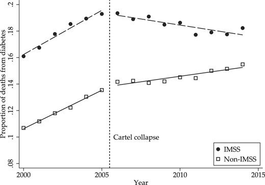
Proportion of deaths due to diabetes, 2000–2014.
Table 6 shows the estimated DiD hazard ratio |$\exp (\beta _4)$| from the proportional hazards diabetes-specific mortality model. Column (1) includes controls for state, year, and insurance coverage, while column (2) adds controls for education and occupation.38 Following the analysis of Section 4.2, uninsured individuals are omitted and an interaction term for post-cartel SSPS coverage is included to isolate the control group of other social security health insurance. The estimated hazard rate associated with the cartel’s collapse is statistically significant and less than one, indicating a reduction in the rate of death due to diabetes following the cartel’s collapse. The estimate corresponds to a per-year reduction in the probability of diabetes-related mortality of 3.4%.
Effect of cartel collapse on diabetes-specific mortality hazard rates.
| (1) | (2) | |
|---|---|---|
| DiD hazard ratio | 0.966 | 0.954 |
| p-value | |${(0.000)}$| | |${(0.000)}$| |
| Education | X | |
| Occupation | X | |
| Observations | 4,051,016 | 3,059,789 |
| (1) | (2) | |
|---|---|---|
| DiD hazard ratio | 0.966 | 0.954 |
| p-value | |${(0.000)}$| | |${(0.000)}$| |
| Education | X | |
| Occupation | X | |
| Observations | 4,051,016 | 3,059,789 |
Notes: Difference-in-differences hazard ratio for diabetes-specific mortality risk. Controls included in both specifications are sex, insurance, state, and year fixed effects. Score bootstrap p-values are reported below each estimated hazard ratio.
To gauge the overall mortality effects of the cartel, I use the estimated effect to calculate the total number of premature deaths due to diabetes that occurred over the cartel period. I define premature death as an individual who would have lived until at least the following calendar year had the cartel never operated. This number is calculated by applying the per-year reduction estimate in column (1) of Table 6 to the total IMSS diabetes deaths occurring over this period. From 2003 to 2005, there were 452,795 total deaths among IMSS beneficiaries, of which 85,692 were due to diabetes. Applying the proportional reduction of 0.966 to these diabetes deaths yields the prediction that 82,778 deaths would have occurred in the same year absent the cartel. The difference between this prediction and realized diabetes deaths implies that the lack of insulin availability created by the cartel caused 2,913 premature deaths or 971 premature deaths per year of the cartel’s operation.
Finally, I re-estimate the model of column (1) of Table 6 with separate IMSS |$\times$| Year interaction terms to examine the evolution of the effect on mortality over time and to test for the presence of pre-trends in diabetes mortality hazard rates. Figure 3 displays these estimated hazard ratios for 2003–2014, using the pre-cartel period as the base category. The first three years correspond to the cartel period, during which there is no observable trend or statistically significant effect. Diabetes mortality increased in the years after the cartel’s collapse before a pronounced downward trend in mortality rates emerged in 2009. The lag between the collapse of the cartel and the decline in diabetes mortality is consistent with the long-term nature of outcomes associated with poor management of diabetes.
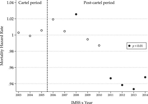
IMSS diabetes mortality hazard rates, 2003–2014.
4.4. Discussion
The utilization and diabetes complications results are large relative to previous studies that focus on developed countries, while the increased mortality risk estimates are comparable to the existing literature on increased pharmaceutical availability. Many studies on how expanded access to pharmaceuticals affects utilization, health outcomes, and mortality use the enactment of Medicare Part D in the United States, which expanded health care coverage to include prescription pharmaceuticals for individuals 65 and older starting in 2006. Estimates for the effect of this program on the increase in utilization in Lichtenberg and Sun (2007) and Yin et al. (2008) suggest that Medicare Part D increased utilization by 13% and 5.9%, respectively, well below the 42% increase in insulin utilization associated with the cartel’s collapse.
The effects of the increased utilization on health are also large relative to existing studies. Again drawing upon the enactment of Medicare Part D, Hanlon et al. (2013) find no improvement in cholesterol levels despite increased utilization of cholesterol-lowering medications. Specifically related to diabetes complications, Simpson, Lin, and Eurich (2016) find a 4% decrease in the risk of developing new diabetes complications associated with medication adherence in the United States.
Previous studies on how access to pharmaceuticals affects mortality have provided mixed evidence. The most related study for insulin availability on diabetes mortality is Américo and Rocha (2020), which studies the effect of subsidies for insulin in Brazil and finds evidence of a decline in hospitalizations but only weak effects on mortality. In studies using Medicare Part D, Kaestner, Schiman, and Alexander (2019) find no effect on mortality, while Huh and Reif (2017) estimate a lower mortality risk driven by reduced risk of cardiovascular death. Dunn and Shapiro (2019) echo this finding of reduced cardiovascular mortality and estimate that Medicare Part D prevented between 7,000 and 26,000 premature deaths out of 34.53 million individuals over 18 months. These estimates imply reduced deaths per million of between 205 and 764. The additional 569 deaths per million over the same period implied by the IMSS mortality estimates lies in the middle of this range.39 One caveat is that the nature of Medicare Part D requires a focus on individuals age 65 and older. In contrast, the mortality analysis for the IMSS diabetic patients applies across the entire age distribution. Restricting attention to individuals above age 65 may yield a different rate of additional premature deaths.
The benefits of eliminating the IMSS insulin cartel were amplified by institutional factors in Mexico, including the high prevalence of diabetes, low insulin utilization relative to high-income countries, and other factors. Market design changes similar to those implemented by IMSS are likely to have the most significant impact in countries facing similar circumstances, such as the treatment of AIDS in many African countries. However, they may have smaller effects in high-income countries where treatment availability is high.
4.5. Placebo, Robustness, and Selection tests
Placebo Tests and Parallel Trends Robustness.
Testing for pre-trends in insulin utilization: Using data from the 2000 ENSA survey, a precursor to the ENSANUT survey, I conduct a placebo test that categorizes 2000 as the pre-intervention period and 2006 as the post-intervention period.40 This test investigates whether insulin usage among IMSS beneficiaries was already increasing relative to other insurance groups in the years leading up to the collapse of the cartel.41 A positive and significant coefficient would indicate that existing trends likely drove increases in insulin usage in the post-cartel period among IMSS diabetics rather than the price change resulting from the cartel’s collapse. The results of these tests are reported in Panel A of Table 7, where column (1) includes base controls and column (2) adds health controls. The estimated coefficients are both low in magnitude and statistically insignificant, suggesting that the main results are not due to differences in pre-trends leading up to the fall of the cartel.
Placebo tests.
| (1) | (2) | |
|---|---|---|
| Panel A: Insulin usage 2000 vs. 2006 | ||
| IMSS |$\times$| 2006 | 0.009 | 0.009 |
| p-value | |${(0.709)}$| | |${(0.739)}$| |
| 95% CI | |$[ -0.16, 0.03]$| | |$[ -0.14, 0.04]$| |
| Base controls | X | X |
| Health controls | X | |
| Observations | 4,145 | 4,145 |
| (3) | (4) | |
| Panel B: Other treatment | ||
| DiD coeff. | |$-0.004$| | |$-0.004$| |
| p-value | |${(0.898)}$| | |${(0.901)}$| |
| 95% CI | |$[ -0.04, 0.21]$| | |$[ -0.04, 0.19]$| |
| Base controls | X | X |
| Health controls | X | |
| Observations | 5,773 | 5,773 |
Notes: Difference-in-differences coefficients for placebo tests on insulin utilization (Panel A) and adherence to nutrition plans (Panel B). For control definitions, see Table 4. Wild cluster bootstrap p-values and confidence intervals are reported below each coefficient.
Possible contamination from other policy changes: My DiD estimation strategy exploits the collapse of a cartel due to market design changes. One issue that needs to be addressed is whether these results might be due to other policies overlapping with the period covered in the data. While restricting the control group to consist only of other social security programs eliminates many sources of policy contamination, such as the Seguro Popular expansion, the presence of other policies with differential effects across the various social security programs constitute a potential threat to identification.
The primary health care policy change affecting diabetes patients in the social security system during the sample period was the introduction of national diabetes clinical guidelines issued by the Secretary of Health in 2008 (Secretaría de Salud 2008), which included specific updates to treatment recommendations (e.g., Kuri Morales et al. 2007). These clinical guidelines aimed to reduce adverse health outcomes resulting from diabetes, cardiovascular disease, and other non-communicable diseases and were published in 2008 with the goal of improving outcomes by 2012. All clinical recommendations issued by the Secretary of Health are national, unified guidelines authored by physicians from all leading public health care organizations. The main identifying assumption is that these clinical guidelines affected social security health care programs in the same way, that is, this program did not interact with IMSS differently than with other social security programs.
To investigate the suitability of this assumption, I perform a placebo test that estimates the DiD specification using another diabetes treatment, adherence to a nutrition plan, as the outcome variable. The use of nutrition plans are included in clinical guidelines for effectively managing diabetes, and the use of nutrition plans increased from 29% in 2006 to 36% in 2012. The recommendation of these plans by physicians and other medical professionals is unlikely to have been affected by the collapse of the insulin cartel. A significant increase in adherence to these plans among IMSS beneficiaries may signal that overall improvements to IMSS diabetes care relative to other health organizations drive the main results. Specifications (3) and (4) in Panel B of Table 7 report the tests of this hypothesis, where specification (3) includes base controls and specification (4) adds health controls. The estimated coefficients are neither large in magnitude nor statistically significant, providing evidence that the results are not due to overall increases in IMSS diabetes treatment quality.
Robustness to functional form: An additional way to examine parallel trends is to test the robustness of the results to different functional form specifications of the parallel trends assumption. As noted in Kahn-Lang and Lang (2019), different functional form assumptions in the regression specification effectively change the formulation of the parallel trends assumption. For instance, when the outcome variable has a log specification, the associated assumption is that trends are parallel as a proportion. In contrast, with a linear specification, the parallel trends assumption requires that the trends are parallel in levels. Varying the functional form used in estimation examines the robustness of the results to different versions of the parallel trends assumption. Table 8 shows the results of tests that vary the functional form of the regression for each outcome variable of Table 4. Column (1) presents the DiD coefficient with insulin use as the outcome variable when using a probit specification. 42 Column (2) shows the results with a logit specification. Finally, columns (3) and (4) show similar tests varying the functional form for the number of complications from diabetes, with column (3) showing the results using Poisson regression and column (4) using a log specification.43 The results show that the main results are robust to different formulations of the parallel trends assumption.
Robustness tests—functional form.
| Insulin | Complications | |||
|---|---|---|---|---|
| (1) | (2) | (3) | (4) | |
| Probit | Logit | Poisson | Log | |
| DiD coeff. | 0.296 | 0.473 | |$-0.314$| | |$-0.152$| |
| p-value | |${(0.032)}$| | |${(0.040)}$| | |${(0.047)}$| | |${(0.023)}$| |
| Base controls | X | X | X | X |
| Health controls | X | X | X | X |
| Observations | 5,307 | 5,307 | 5,773 | 5,773 |
Notes: Difference-in-differences coefficients for the effect on insulin utilization and diabetes complications that mirrors Table 4 with changes to functional form. For control definitions, see Table 4. Score bootstrap p-values (columns (1)–(3)) or wild cluster bootstrap p-values (column (4)) are reported below each coefficient.
Other Robustness Checks.
Table 9 displays the results of other robustness checks, which include the addition of medical variables correlated with diabetes severity, separate effects by survey wave, and restring the sample to individuals diagnosed with diabetes prior to the cartel’s collapse.
Robustness checks for medical variables, time effects, and diabetes duration.
| Insulin | Complications | |||||||
|---|---|---|---|---|---|---|---|---|
| (1) | (2) | (3) | (4) | (5) | (6) | (7) | (8) | |
| DiD coeff. | 0.056 | |$-0.314$| | ||||||
| |${(0.031)}$| | |${(0.021)}$| | |||||||
| IMSS |$\times$| 2012 | 0.040 | 0.049 | 0.056 | |$-0.305$| | |$-0.316$| | |$-0.321$| | ||
| |${(0.030)}$| | |${(0.022)}$| | |${(0.026)}$| | |${(0.034)}$| | |${(0.029)}$| | |${(0.024)}$| | |||
| IMSS |$\times$| 2016 | 0.090 | 0.083 | 0.064 | |$-0.276$| | |$-0.305$| | |$-0.153$| | ||
| |${(0.098)}$| | |${(0.052)}$| | |${(0.429)}$| | |${(0.150)}$| | |${(0.112)}$| | |${(0.279)}$| | |||
| Base controls | X | X | X | X | X | X | X | X |
| Health controls | X | X | X | X | X | X | X | X |
| Diabetes controls | X | X | X | X | X | X | ||
| Pre-2006 diag. | X | X | ||||||
| Observations | 5,618 | 5,773 | 5,618 | 4,079 | 5,618 | 5,773 | 5,618 | 4,079 |
Notes: Difference-in-differences coefficients for robustness checks that include diabetes medical controls for the base specification (columns (1) and (5)), separate year effects (columns (2)–(4) and (6)–(8)), and restricting the sample to individuals diagnosed with diabetes prior to the collapse of the cartel (columns (4) and (8)). For base and health control definitions see Table 4. Diabetes controls are the use of oral diabetes medication and the number of diabetes-related doctor visits per year. Wild cluster bootstrap p-values are reported below each coefficient.
Inclusion of health care and pharmaceutical utilization controls: To avoid the inclusion of potentially endogenous variables, the specifications of Table 4 include only patient-level demographic and health status variables and do not include other factors relating to diabetes care and treatment. However, unobserved factors influencing diabetes severity may be correlated with the treatment group. To examine this, I add diabetes treatment variables correlated with the severity of diabetes to the main specifications. These include the frequency of diabetes-related medical visits and the use of oral anti-diabetic medications. Table 9 reports the results of these tests. The estimates remain statistically significant and similar in magnitude to the main results.
Separate time effects: Columns (2)–(3) and (6)–(7) of Table 9 show the estimated effects for the 2012 and 2016 ENSANUT waves separately, first with base controls and health controls and then adding diabetes medical controls defined above. The most precise estimates are obtained for the 2012 wave, the first survey wave after the cartel’s collapse. The point estimate on insulin usage for 2016 is much higher but is only marginally significant at 10%. The effect on complications is similar across the 2012 and 2016 surveys, but as with the effect on insulin utilization, the estimate becomes less precise for the latter year.
Restricting to diabetes patients with pre-cartel collapse diagnosis: One potential threat to identification is that IMSS responded to the collapse of the cartel by increasing resources dedicated to detecting and diagnosing diabetes. If newly diagnosed cases within IMSS are less severe than previously diagnosed cases, then the main results of Table 4 might reflect this compositional change rather than the direct effects of the cartel’s collapse.
While the subsequent section tests for additional diagnoses directly using MXFLS data, it is also possible to test for the effects of newly diagnosed diabetes patients on the main results using the ENSANUT data by restricting the sample to cases diagnosed before the cartel’s collapse. Because this sample consists of those already having a diabetes diagnosis when the cartel collapses, the effects cannot be due to compositional effects resulting from newly diagnosed patients. Columns (4) and (8) of Table 9 show the results from this specification with estimates similar to the main results, suggesting that new diagnoses are not driving the results.
Additional robustness checks:Online Appendix E contains further robustness checks. Robustness checks on insulin utilization and diabetes complications include dropping all individuals affiliated with SSPS or the private health care system in the main specifications of Table 4 and adding the 2000 ENSA data to the full sample in the placebo analysis of Table 7.
For the mortality analysis, Online Appendix E examines the sensitivity of the results to incorporating competing causes of death. This specification adds cardiovascular disease as a competing mortality risk following the model of Fine and Gray (1999). None of the results are significantly affected by these specifications.
Patient Selection, Diabetes Diagnoses, and out-of-Pocket Expenditures.
Lastly, I perform a series of tests on the assumptions of the DiD models estimated in previous sections using the longitudinal data from MXFLS. Specifically, I test for patient selection to examine whether diabetes patients were more likely to switch to IMSS following the cartel’s collapse, changes to diabetes diagnoses to test whether IMSS became more likely to diagnose diabetes after the cartel, and how out-of-pocket expenditures for diabetes medication changed for individuals in IMSS relative to other social security groups.
Although the results are robust to controlling for observable individual characteristics, including additional diabetes treatment variables, I also examine whether diabetes patients were more likely to switch to IMSS coverage following the cartel’s collapse. This test tracks individuals with non-IMSS coverage before the collapse and assigns a dependent variable equal to one if the individual switched to IMSS after the collapse. The DiD framework for this specification compares individuals diagnosed with diabetes prior to the fall of the cartel to those who were never diagnosed with diabetes and hence tests whether diabetic patients with non-IMSS social security coverage were more likely to switch to IMSS coverage than non-diabetics. A positive and significant effect would suggest that individuals with diabetes selected into IMSS coverage following the cartel’s collapse, likely by finding employment in the formal sector. Column (1) of Table 10 gives the result of this test, which shows a statistically insignificant effect of having diabetes on switching to IMSS coverage. The result suggests that selection into IMSS coverage is not common; this is perhaps not surprising because changing to IMSS requires a change in employment by a household member, meaning that a change in job, employment sector, or location is required.
Effect of cartel collapse on insurance switches and diabetes diagnoses.
| (1) | (2) | |
|---|---|---|
| DV: Switch to IMSS | DV: Diabetes diagnosis | |
| Sample: non-IMSS beneficiaries | Sample: non-diabetics | |
| Diabetes |$\times$| Post | 0.023 | |
| IMSS |$\times$| Post | 0.010 | |
| p-value | |${(0.492)}$| | |${(0.260)}$| |
| 95% CI | |$[ -0.04, 0.09]$| | |$[ -0.18, 0.13]$| |
| Base controls | X | X |
| Health controls | X | X |
| Observations | 11,349 | 10,148 |
Notes: Difference-in-differences coefficients, which test for effects on the cartel’s collapse to cause diabetic patients covered by other insurers to switch to IMSS coverage (column (1), dependent variable mean is 0.15) and whether individuals within IMSS were more likely to be diagnosed with diabetes relative to other insurance groups after the cartel’s collapse (column (2), dependent variable mean is 0.04). Base controls are age, sex, height, weight, waist circumference, and fixed effects for insurance, survey wave, employment, education, and municipality. Health controls are smoking, hypertension, heart disease, and alcohol use fixed effects. Wild cluster bootstrap p-values and confidence intervals are reported below each coefficient.
Secondly, I also test whether individuals within IMSS were more likely to be diagnosed with diabetes conditional on individual characteristics. This test uses the sample of all individuals without diagnosed diabetes in 2005 and compares individuals in IMSS to those with non-IMSS social security insurance. A positive and significant effect would suggest that the composition of individuals within IMSS changed due to, for example, the reallocation of resources previously spent on high-priced insulin toward additional diabetes testing and diagnosis efforts. This constitutes a potential threat to identification, as those diagnosed with diabetes due to these new efforts may have unobservable factors correlated with diabetes severity. Column (2) of Table 10 displays the results of this test. I find no significant effect of those with IMSS being more likely to be diagnosed with diabetes.
Finally, I test whether individuals in IMSS saw their out-of-pocket expenditures for diabetes medications decline after the cartel’s collapse.44 Given the paucity of information on procurement outcomes for other public health care providers, this serves as a check that the increase in insulin usage for IMSS diabetes patients is due to increased availability and not changes to prescribing behavior by IMSS physicians. Because medication shortages may prompt individuals covered by public health insurance to purchase medication from the private sector (Gidi 2010), a negative effect on out-of-pocket diabetes medication expenditures among IMSS diabetes patients would indicate an increase in medication availability. Table 11 presents the results of this test, where column (1) uses a sample consisting of individuals who used diabetes medication in 2005, while the sample used in the specification for column (2) consists of all diabetic patients. The negative coefficients for IMSS out-of-pocket expenditures following the collapse of the cartel indicate that medication availability increased relative to those with other public social security health insurance, reinforcing the results of Section 4.2.
Effect of cartel collapse on diabetes medication expenditures.
| (1) | (2) | |
|---|---|---|
| Used diabetes medication in 2005 | All diabetic patients | |
| DiD coefficients | |$-230.015$| | |$-56.180$| |
| p-value | |${(0.041)}$| | |${(0.037)}$| |
| 95% CI | |$[ -1092.46, -172.74]$| | |$[-559.77, -11.92]$| |
| Base controls | X | X |
| Health controls | X | X |
| Observations | 917 | 1,547 |
Notes: Difference-in-differences coefficients with the inclusion of diabetes treatment variables. Dependent variable is quarterly diabetes expenditures in Mexican pesos. The pre-treatment mean of the dependent variable for all diabetes patients, column (2), is 297. For control definitions, see Table 10. Wild cluster bootstrap p-values and confidence intervals are reported below each coefficient.
5. Conclusion
In this paper, I show that the market power wielded by a pharmaceutical cartel restricted the supply of insulin to a significant public health care provider and contributed to adverse health outcomes. Straightforward policy changes motivated by economic theory successfully stopped the cartel and improved access to diabetes treatment. Estimates of diabetes-specific mortality indicate that the shortage of insulin caused by the cartel contributed to 971 premature deaths annually.
Broadly, this study informs the evaluation of damages caused by cartels. Evaluating direct consumer harm, such as worsened health outcomes and increased mortality risk, provides a new way to measure the detrimental effects of collusion beyond price-theoretic welfare evaluations for intermediate goods that currently dominate the literature. While the direct monetary effects of the insulin cartel were substantial, including detrimental health effects and premature deaths significantly increased the appraisal of the damages generated by the cartel.
The effectiveness of IMSS policy changes in stopping collusion also informs the debate on how best to achieve equitable outcomes in lower- and middle-income countries. Markets in these countries are often beset by the problem of weak institutions, such as weaker competition authorities relative to developed nations (Bradford and Chilton 2018). Market design is gaining attention as a means to combat weak institutions and alleviate inequality (Kominers, Teytelboym, and Crawford 2017, Roth forthcoming). Recent discussions on the role of contracts and institutions in allocating health care resources within developing nations, particularly vaccines for COVID-19 (Phelan et al. 2020), further enforce the importance of market design. The empirical results of this paper provide evidence that well-designed markets are crucial in achieving equitable outcomes.
While the ability of changes in market design to stop collusion is encouraging, the results paint a bleak picture of the potential for market power to disrupt the health and well-being of individuals. Much less is known about the functioning of markets in developing countries than in developed nations, often due to limited data availability. However, concerns of market disruption due to corruption and collusion are rife. Better understanding the propensity for these market inefficiencies to generate shortages in such goods as medicines, food, and housing will inform policies that enhance access to these necessities.
Acknowledgments
I thank the editor, Pierre Dubois, and four anonymous referees. I am also grateful to John Asker, David P. Byrne, Zhijun Chen, Simon Loertscher, Robert A. Miller, Kole Reddig, Regina Seibel, and participants during presentations at Monash University, the Hal White Antitrust Conference, the University of Melbourne Centre for Market Design, International Industrial Organization Conference, Asian Meeting of the Econometric Society, and Australasian Meeting of the Econometric Society for providing comments and Samuel Vazquez for providing information on IMSS purchases.
Notes
The editor in charge of this paper was Pierre Dubois.
Footnotes
IMSS procurement contracts stipulate a minimum purchase quantity and may include the option to purchase additional units over the contract’s duration. An analysis of the legal proceedings conducted by the Mexican competition authority contains data on average realized insulin purchases per year over the cartel period of 2003–2005 (Comisión Federal de Competencia Económica 2015b).
For example, antitrust violations drew paltry fines even for substantial infractions, and antitrust regulators were limited in the information they could obtain during an investigation without the investigated firm’s knowledge or consent. Section 2 elaborates.
Dubois, Lefouili, and Straub (2021) study the effects of centralized procurement on drug prices in low- and middle-income countries and find that centralization leads to lower prices but that higher industry concentration attenuates the price reduction. I document substantial price declines after consolidation, suggesting that market concentration and firm conduct may interact separately with centralization policies.
Formally, there are two component programs under the umbrella of IMSS: the main program, IMSS, which covers the vast majority of individuals, and IMSS Oportunidades, which focuses on the indigenous and marginalized populations of Mexico and has a much lower enrollment.
In the econometric specification, detailed in Section 4.1, the control group is comprised of these non-IMSS social security programs, while the treatment group contains IMSS individuals.
Individuals with type 1 diabetes, in which the pancreas produces little or no insulin at all, will require insulin therapy from the time of diagnosis. Type 2 diabetes, in which the body becomes resistant to insulin, often does not require immediate insulin therapy and can be managed with various treatments.
The Secretary of Health published the first set of national clinical guidelines for diabetes treatment in 1994, with updates in 2001 and 2007. All guidelines include recommendations for insulin prescription based on biomarker targets.
The CFC was the primary competition regulatory authority in Mexico until 2013, when it was replaced by the Comisión Federal de Competencia Económica (Cofece).
This corresponds to a first-price sealed-bid procurement auction where all firms have constant costs c and the auctioneer buys q units with a reserve price of v.
For simplicity of notation, the dependence of T on |$\delta$| and I is suppressed. This dependence and its implications are made more explicit in Online Appendix A.
Table A.1 in Online Appendix A gives a timeline of events for the insulin market for the investigation.
Estrada and Vazquez (2013) document the price effects across pharmaceutical markets that triggered an investigation by the CFC.
Dimesa first participated in January 2006 and frequently under-bid the cartel members. Dimesa submitted a bid lower or equal to the lowest cartel member bid in all but eight auctions in 2006. However, during this period, Dimesa frequently tied exactly with one or more cartel members.
One firm fined for bid-rigging in the market for saline solutions, Baxter, was successful in overturning their fine upon judicial review, perhaps revealing the risky nature of the legal strategy pursued by the CFC.
Monetary damages are calculated as the difference in price before and after the cartel at the total quantity purchased during the cartel period. A back-of-the-envelope calculation for indirect monetary damages arising from increased diabetes complications treatment costs is contained in Online Appendix A.
Even the most conservative estimate for quantity increases, comparing the upper quantity range in 2005 with the lower quantity range in 2007, indicates a 42% increase in insulin purchases. While the data are not suitable for precise estimates of demand elasticities, as done in Einav, Finkelstein, and Polyakova (2018), this represents evidence that purchase quantities are sensitive to prices at an institutional level.
The medical literature provides evidence that incomplete adherence to recommended insulin treatment increases complication risk (Khunti et al. (2017)).
These indirect effects are difficult to measure, as detailed patient treatment data, such as treatment of diabetes complications, is not available. The following sections focus on the direct effects of the cartel on insulin utilization and observable diabetes health outcomes and leave the study of the effects of resource reallocation in the aftermath of the cartel to future work.
Ley de Adquisiciones, Arrendamientos y Servicios del Sector Público, original version available at http://www.dof.gob.mx/nota_detalle.php?codigo=2049070&fecha=04/01/2000.
Specifically, purchases are conducted using first-price sealed-bid auctions with a reserve price set by the procurement authority. Regulations on bidding, such as how bids are submitted and how auction results are revealed to participants, are the same across social security procurement practices.
The successful prosecution of the cartel also prompted reviews of procurement practices across social security programs in Mexico in coordination with OECD guidelines (OECD (2011, 2013)). IMSS had already implemented many OECD recommendations, such as procurement consolidation and reducing entry barriers for international competitors. ISSSTE began implementing similar changes in 2012, including plans to further consolidate purchases via joint procurement with IMSS. Any price reduction in these markets from the procurement design changes would likely lead to underestimation of the effects of the cartel, as discussed in Online Appendix C.
The survey does not distinguish between Type I and Type II diabetes; the sample consists of all individuals diagnosed with any form of diabetes. Online Appendix B provides additional survey details.
For consistency with the ENSANUT survey, I define adult deaths as occurring at age 20 or later and drop all deaths occurring before age 20 from the estimation sample.
Specifically, the control group consists of members of non-IMSS social security programs, which includes ISSSTE, the sector-specific program PEMEX for oil and gas workers, military members, and state-level programs covering state government employees. In the ENSANUT data, this excludes (i) individuals who primarily use private health care and (ii) individuals enrolled in SPSS/Seguro Popular. The treatment group consists of individuals enrolled in IMSS or IMSS Oportunidades. As IMSS Oportunidades has a separate provider network, I treat these as separate insurance programs that were both subject to the treatment.
Online Appendix D shows the results of alternative econometric specifications, including variation to the control group and various matching-based estimators.
In the empirical analysis, I include all insured individuals and include time interactions with private health care and SPSS coverage to isolate the treatment and control groups; Online Appendix E shows results when other insurance groups are excluded entirely.
The difficulty of accurate inference with small number of clusters has been noted by Bertrand, Duflo, and Mullainathan (2004) and Conley and Taber (2011). MacKinnon and Webb (2017) demonstrate that when the number of treated clusters is small in DiD designs, there is a severe tendency to under-reject the null hypothesis when the restricted wild cluster bootstrap is used (that is, when the null hypothesis is imposed on the bootstrap DGP). I use only the restricted version of the wild cluster bootstrap, which suggests that the associated p-values for these specifications can be interpreted as conservative estimates of statistical significance tests. The results are robust to various clustering methods, with the wild cluster bootstrap yielding the most conservative p-values.
Because of the computational burden associated with generating confidence intervals using the score bootstrap, only p-values are reported for these results.
Online Appendix B describes the classification of deaths by cause.
The slope of the proportion of non-IMSS diabetes deaths flattens slightly in the post-cartel period. This may be due to programs such as the updated national clinical guidelines for diabetes, discussed further in Section 4.5. The primary identifying assumption is that these national programs would impact the slope of both non-IMSS and IMSS diabetes deaths in the same way, absent the cartel’s collapse.
The diabetes-specific mortality proportional hazards model treats other causes of death as independent censoring. In Online Appendix E, I relax this assumption by treating cardiovascular disease as a competing cause of death and find similar results.
Because INEGI changed occupation classifications in 2013, the specification in column (2) uses the sample through 2012.
This figure is reached by dividing the 2,913 total deaths over three years into 18 months, yielding 1,456.5 total deaths, and dividing this figure across the estimated number of IMSS diabetic patients in 2005 calculated from the ENSANUT survey data.
Specifications, which add the 2000 ENSA survey to the full data set and include Year|$\times$|IMSS interactions generate similar results; see Online Appendix E.
It is not possible to perform a similar test using complications as the dependent variable as complications from diabetes are not recorded in the 2000 edition of the ENSA survey.
The probit specification assumes that in the counterfactual of no intervention, the treatment and control groups would have moved by the same number of standard deviations of the normal standard error.
Specifically, the transformed outcome variable is |$\log (1+$| Number of Complications).
The MXFLS data contains the amount spent on all diabetes medications, not insulin specifically. Because this amount also includes any expenditures on oral anti-diabetic medication, this serves as a noisy measure of insulin availability.
