


Abstract
This paper studies consumers’ choice between two different water tariffs. We document a large inaction in a novel setting where customers face a binary decision and receive simple, detailed, and personalized information about the financial savings they would obtain if they were to switch water tariff. Our empirical framework separates two sources of inertia: inattention and switching costs. The model estimates that half of the customers that would benefit from changing tariff are not aware of the opportunity they are offered. Conditional on paying attention, we estimate median switching costs to be around £100. A model where all customers are assumed to pay attention delivers instead implausibly high switching costs, with a median of £400. This shows the importance of inattention in explaining consumers’ inaction. Looking at the characteristics of the households, our results confirm previous findings that areas where households have higher levels of education or the proportion of minorities is lower display a higher responsiveness to potential savings. The new insight offered by our analysis is that this is entirely driven by attention, whereas switching costs actually increase with education and ethnic homogeneity. Our findings suggest that policies aimed at increasing attention can play a central role in fostering competition among suppliers and reducing inequalities.
A set of Teaching Slides to accompany this article are available online as Supplementary Data.
1. Introduction
There is increasing evidence that people often fail to take actions that would benefit them financially. For instance, Keys, Pope, and Pope (2016) find that approximately 20% of U.S. households failed to take advantage of lower rates by refinancing their mortgage, with a median present-discounted cost of $11,500. Two different but not mutually exclusive explanations can justify the pervasiveness of this behavior: Some individuals may fail to consider the potential gains, because they do not pay attention, while some others may assess that the gains are not worth the hassle. Spending time and effort to gain a few dollars may well be reducing utility, whereas forfeiting an opportunity because of unawareness implies that the benefits may be worth the costs, but individuals do not have the information to make such comparison. Understanding the source of inaction is important to define more effective policies to encourage consumers to take action, with the aim of, for instance, increasing competition among firms or decreasing inequalities. For example, simplified application processes for social benefits may be effective if the main barrier for applicants is transaction costs, but may not be so effective if the main issue is instead lack of attention.
In this paper, we examine the choice of water tariff among more than 225 thousands households in the southeast of England. Between 2010 and 2015, a compulsory metering program saw the installation of water meters in all houses where it was technically feasible. Soon after installation, households were moved by default to the new metered tariff. However, they were also offered the possibility to pay for 2 years a transitional tariff, called changeover tariff, a combination of the metered tariff and the “old” unmetered tariff, based solely on the characteristics of the house. What we uncover is a massive inaction by consumers, who for the most part fail to take advantage of the option and, as a result, end up paying higher water bills, losing on average £121 (median £83). This despite consumers face a rather simple binary choice, whose financial implications are clearly communicated and which requires only a telephone call.
To understand the sources of consumers’ inertia, we define a simple empirical framework whereby the probability that a household takes advantage of the changeover tariff depends on two different elements: attention and switching costs. The former refers to the likelihood that households are aware of the changeover tariff, having read and understood its characteristics, while the latter refers to the probability that, conditional on paying attention, the benefits from changing contract are higher than the latent costs of requesting the switch of tariff. In this respect, our work is related to those by Heiss et al. (2021) and Drake, Ryan, and Dowd (2022), which investigate the relative importance of inattention and switching costs in explaining consumers’ inertia in health plan choices. However, in our study, customers are facing a simple binary choice in a setting where the costs of obtaining and processing the information about financial gains and of carrying out the switch can be expected to be considerably lower than those involved with the health plan choice. Furthermore, the identification strategies they use to estimate the two sources of inertia are very different from the one we use in this paper. In Heiss et al. (2021), identification relies on two fundamental exclusion restrictions: The attention stage excludes information on new plan features that are not observed by inattentive consumer, while the plan-choice stage excludes past information that is irrelevant for the new enrolment period. In Drake, Ryan, and Dowd (2022), latent inattention is identified in part through demand asymmetry (Abaluck and Adams-Prassl 2021) and in part using an exclusion restriction similar to Heiss et al. (2021). Drake, Ryan, and Dowd (2022) also use a second approach that exploits the fact that they can observe whether households actively selected their health plan—and so they know these households paid attention—or chose to automatically re-enrol in their default option. Differently from these two papers, our identification strategy makes use of a particular feature of our data, namely the fact that each household receives information about the specific financial gains they could obtain if they decide to adopt the changeover tariff: information that we assume does not affect the probability of attention because the financial gains are revealed only after a household reads the documents notifying them about the existence and structure of the tariff. In other words, customers can learn about their potential financial gains only by paying attention and, therefore, we assume that these gains are excluded from the attention stage.
To gauge the importance of modeling inattention, we estimate first a restricted model assuming that everyone is aware of the alternative tariff. Using this model, we estimate the median switching costs to be about £400, an amount unrealistically high considering the low effort required to adopt the changeover tariff, that is, making a telephone call. However, in a full model that allows for inattention as an additional source of inertia, the median switching costs are estimated at a more reasonable figure of around £100. Furthermore, we show that around 50% of households that gain financially from moving to the changeover tariff fail to take action because of inattention. Compared with an unconditional probability of switching of 24%, emerging from the restricted model, we find that, conditional on paying attention, the probability of switching is a much higher 56%. While the exact magnitude of switching costs is of course context-specific, these figures bring evidence of the importance of inattention in explaining consumer inaction. Given that the promotion of an increase in competition among suppliers is a centrepiece of market regulation, in particular for utilities, and that, to be effective, this needs active consumers, our empirical analysis suggests that policies aimed at increasing attention are particularly important.
This paper contributes to a growing literature documenting and explaining the root causes of consumers’ inaction.1 This has been observed in a variety of settings, including health insurance markets (Handel and Kolstad 2015), retirement plans (Madrian and Shea 2001; Benartzi and Thaler 2007), and electricity (Fowlie et al. 2021). In the context of water (and energy) consumption, a paper by Tiefenbeck et al. (2016) shows the importance of inattention by consumers and the importance of saliency through an experiment with real-time feedback during showering.2 As explained in Section 2, we study inaction in an environment where customers face a simple binary decision, potential gains are clearly explained, there is no role for brand loyalty and preferences for unobserved product characteristics. Thus, many potential explanations for inaction (e.g. search costs, choice overload, lack of salience, and status quo bias) are unlikely to play a role. Furthermore, the simple decision setting and the provision of personalized information makes identification of the relative importance of inattention and switching costs cleaner compared with other studies that have focused on more complex settings (e.g. Heiss et al. 2021).
We also explore how different demographic characteristics are associated with the observed inaction, a topic of high relevance for policy-making, because of its equity implications.3 A higher level of inaction among poorer households compared with better-off ones, for instance, regarding access to benefits, may make a policy regressive in its practical effects despite not being so in its design. We use a rich dataset combining billing data and customers’ information with data on income, education, and ethnicity at the neighborhood level to investigate how these characteristics affect the probability of being attentive as well as the switching costs associated with the adoption of the changeover tariff. Our results confirm previous findings that areas where households have higher levels of education or the proportion of minorities is lower, display a higher responsiveness to potential savings. Letzler et al. (2017) exploit a natural experiment about a fraudolent subscription program where letters providing the opportunity to cancel are sent to consumers. They find that “[c]onsumers from low socio-economic status (SES) neighbourhoods and racial and ethnic minorities were even less likely to respond to the notification letters than consumers from higher SES communities and consumers who were likely to be white”. Beshears et al. (2015) study 401(k) plans and find lower opt-out odds for the low-income group, as well as for younger employees. Bhargava, Loewenstein, and Sydnor (2017) find that low-income employees are significantly more likely to choose dominated health plan. Also, Hortaçsu, Madanizadeh, and Puller (2017) find evidence of inaction being larger in “neighbourhoods with lower income, lower education, and more senior citizens”. Sahari (2019) find a low sensitivity by low-income households to energy costs at the moment of making a long-term energy technology investment. The new insight offered by our analysis is that the higher responsiveness to potential savings by households living in more educated and homogeneous areas is entirely driven by a higher probability of paying attention, whereas switching costs actually increase with education and homogeneity.4
The rest of the paper is organized as follows. Section 2 describes the institutional setting, providing details regarding the tariff, the timing of the choice, and the information given and received by customers, as well as highlighting how, in light of the existing literature, several institutional features should be conducive to an active choice by consumer. Section 3 presents our econometric framework and identification strategy, while Section 4 describes our data and provides some descriptive empirical facts about the uptake of the changeover tariff. The estimation results are presented and discussed in Section 5. Section 6 concludes by discussing the policy implications of our findings.
2. Institutional Setting
In this section, we first describe the institutional context in which metering and the changeover tariff took place (Section 2.1). We then document the information provided to customers through the different stages of the metering process (Section 2.2) and explain the customers actual experience on the basis of qualitative research (Section 2.3). Finally, in Section 2.4, we discuss how, in light of the existing literature, this institutional setting presents several characteristics that should minimize inaction.
2.1. Metering and the Changeover Tariff
First of all, we provide some background information to understand the utility incentives. The water industry in England and Wales is regulated by Ofwat, a government department established in 1989 when the water and sewerage industry was privatized. Ofwat establishes an overall framework for setting price controls, with the aim of protecting customers from monopoly companies charging more than they need. The price for retail household services covers all relevant costs including a reasonable return on investment made in providing quality services to customers.5 All companies’ charging schemes, including the changeover tariff studied in this paper, are agreed with Ofwat.
The supply area of Southern Water (SW) was designated as an area of serious water stress by the Secretary of State for the Environment Food and Rural Affairs in 2007, and the company was required to consider the case for universal water metering as a cost-effective measure to balance demand and supply. Following public consultation on its plan in 2008, compulsory metering became part of the company’s statutory water resources management plan.
Soon after the approval of Southern Water’s Universal Metering Programme, Ofwat entered into discussion with Southern Water to see how the company could support households with high water use who used to pay a relatively low unmetered tariff. This resulted in the introduction of the changeover tariff, which allowed water bill increases to be phased in over a number of years.6
Being part of the charging scheme, the cost of the changeover tariff in terms of lost revenues was paid by customers through higher tariffs in the following years. As such, applying automatically a changeover tariff to customers that were better-off under such tariff would have meant a higher standard tariff to compensate the water utility for these extra costs. The optional setup finally implemented was cheaper and more targeted, under the—ex ante reasonable but empirically not validated—assumption that lower income households were more likely to call.
Accordingly, the water utility had an interest in raising awareness about the tariff because they did not have to bear the financial consequences, but they could comply with Ofwat’s requirements of improving efficiency in water usage while reducing the financial impact of metering on households.
After providing the background, we now describe in detail the tariffs. The metered tariff consists of a standing charge and a volume charge. The standing charge is a fixed charge based on the size of the meter fitted to the property and covers the costs of maintaining the water services account. The volume charge is based on the amount of water supplied to the home, that is, the volume of water recorded on the meter in each billing period.
The unmetered tariff does not depend on water consumption and consists of a standing charge and a rateable value charge. The standing charge is a fixed amount for all properties and covers the costs of maintaining the water services account. The rateable value charge is based on the rateable value of the house. The rateable value was used as the basis for local authority taxation prior to 1990. Rateable values were set by the Valuation Office (part of HM Revenue and Customs) to reflect the rental value of the property. The rateable value is no longer used for taxation and no longer updated. The water company normally used the rateable value quoted in the Valuation List in force on 31 March 1990.
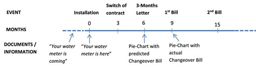
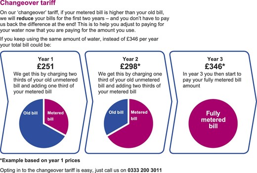
The changeover tariff is valid for 2 years after the switch of contract (see Figure 1), and it consists of a weighted average of the metered and unmetered tariffs described above. More precisely, during the first year after the switch, the changeover tariff is 1/3 of the metered tariff and 2/3 of the unmetered tariff, while during the second year, the bill is 2/3 of the metered tariff and 1/3 of the unmetered tariff.
Typical customer journey.
Customers can opt for the changeover tariff at any point within 2 years of the switch of contract. While theoretically it would be possible to go back to the metered tariff after having opted for the changeover tariff, this option is not advertized, and in our dataset, we do not observe anyone doing that, so we consider the decision to switch as irreversible. We also note that, regardless of when customers decide to opt for the changeover tariff, this is applied for the whole 2-year period.
2.2. Information
Figure 1 summarizes the typical customer journey with the information received at the different stages of the program. Notice that in the UK water bills are usually sent every 6 months. The exact month varies from customer to customer and, in our context, there is variation due to the fact that meters were installed throughout the year.
Approximately 4–6 weeks before installation, customers receive a booklet titled “Your water meter is coming—part 1 of 2”, where the changeover tariff is mentioned.7 A brief mention to a “changeover” period is also present in the leaflet titled “Southern Water’s metering programme” that customers receive approximately 3 weeks before installation and that is also distributed at key locations within the installation area (e.g. post offices, libraries, etc.). On the day of installation, customers receive a leaflet titled “Your water meter is here—part 2 of 2”. Here, the changeover tariff is explained in more details. In particular, customers are informed that about 3 months after installation they will be automatically switched to the new metered tariff and that 6 months after installation, they will receive the so-called 3-months letter “explaining how much water you have used and how much your first metered bill is likely to be if you keep using the same amount of water. You will also be given the choice to opt for our ‘changeover’ period of payment”. Then, they are informed that about 9 months after installation (6 months after switching contract), they will receive their first metered bill and be given a second opportunity to opt for the “changeover” period of payment. Finally, the leaflet explains the changeover period and provides an example based on a rateable value bill of £378 and a would-be fully metered bill of £450. The example is illustrated through a pie chart that shows how adopting the changeover tariff saves money for the customer. (See in the Online Appendix an extract from the installation leaflet explaining the changeover tariff in detail.)
The 3-month letter informs customers about their water usage in the first 3 months after the meter has been turned on. We report a sample in the Online Appendix, underlining in yellow the parts mentioning the changeover tariff. Figure 2 shows the key section of the 3-month letter dealing with the changeover tariff.
Main information in the 3-month letter.
As can be seen, the letter contains a personalized pie chart, with calculations based on the actual unmetered charges applying to the customers and on a projection about metered charges based on the observed consumption in the 3 month period. Thus, customers not only receive information about the main features of the changeover tariff, but also a clear indication of the potential savings arising from it given their specific characteristics. Research by Samek and Sydnor (2017) shows how, in the case of health insurance, moving from describing the features of plans to providing information about their different financial consequences through “consequence graphs” greatly reduces the share of people choosing financially dominated options thanks to improved understanding. In our case, we would thus expect the clear representation of the financial consequences of adopting the changeover tariff to reduce the scope for misunderstanding. In the letter, it is also clearly indicated that customers need to take action in order to adopt the tariff. In particular, under the pie chart it is mentioned how “[o]pting in to the changeover tariff is easy, just call us on 0333 200 3011”. At the end of the page explaining the changeover tariff, there is, moreover, the bright banner reported in Figure 3, making it very prominent that a call is needed to adopt the tariff.

Banner in 3-month letter.
The first bill is sent after a further 3 months and also includes a personalized pie chart, highlighting both the yearly fully metered charge and the changeover charge under the assumption that the customer keeps using the same amount of water. (See Online Appendix for a sample, with parts mentioning the changeover tariff highlighted in yellow.) Also here there are multiple indications that customers need to take action in order to switch to the changeover tariff. Under the pie chart, it is indicated how “[t]he charge for this period of £[personalized amount] is your fully metered charge. If you want to go on our changeover tariff just call 0333 200 3012 and we will send you a revised bill. If you do not contact us you will stay on the standard metered tariff.” There is once again at the end of the page the banner of Figure 3 and, in the following page, after detailing the charges, it is written “This is your first metered bill. For your first four metered bills, when your metered amount is higher than your old bill, you can go on our ‘changeover’ tariff—call 0333 200 3012 to go on this tariff.”
In the bills, the information about the changeover tariff is provided after the heading “Trouble paying? Can you afford it?”, while the changeover tariff could be requested by everyone, regardless of affordability issues. Indeed, the first booklet mentioned above correctly stated “[a]ll our customers will be given the opportunity to choose a ‘changeover’ tariff for paying their water bills”. This language may have deterred some relatively well-off customers from engaging with the tariff. The fact that, as we will see further on, people from more affluent neighborhood were more likely to apply, suggests, however, that this may not have been so common.
2.3. What Customers Experienced
The Consumer Council for Water (CCW),8 the independent representative of water consumers in England and Wales, commissioned in 2013 a report (CCW 2013) about the impact of metering on customers based on a quantitative survey, plus in-depth interviews, and focus groups. A follow up, this time in collaboration with Southern Water and based on a few focus group sessions, took place in 2016 (CCW and SW 2016). The first report highlights several aspects that are of direct relevance for this paper. First of all, the fact that there was widespread inattention among customers, in terms of both completely ignoring information and not understanding it properly. The report, for instance, highlights how “[t]he majority of customers are of the view that Southern Water has provided a large amount of information and even if they have not read it all, feel that the company has made a considerable effort to keep its customers informed. [...] on closer discussion, it emerged that customers are often unclear or have an inaccurate picture about what they can expect with respect to metering and the decisions they have to make”. Also, “[c]ustomers frequently had some understanding that the process of moving onto metered charging was a gradual one that would give them time to get used to it. Many had some appreciation that this involved a delay before their meter reading counted towards their bill and some knew something of the changeover tariff; however, the detail of both of these was often hazy and sometimes incorrect”. More specifically about the changeover tariff “[t]he changeover tariff was rarely known by name although customers sometimes recognised it when prompted; given that there is little about the tariff in the first information booklet and some customers had not read the second, this is perhaps not surprising. While customers had some understanding that it would help keep their bill at a lower level, they tended to be unaware of the mechanism for doing this and often made incorrect or incomplete assumptions about it”. Furthermore, “[t]he mechanism for going on to the tariff was another point of uncertainty with some thinking that they had just a three month window in which to decide if they wanted to opt into it and others thinking that it would be applied to everyone’s bills”. The second report also underlines how “[t]he concept of the ‘changeover tariff’ [...] was also generally well recalled, although metered customers were often vague about the details. Respondents typically understood that there would be a ‘phased’ approach to moving from rated to metered bills, although the detail of this process was not always well understood”. So, even if information was there, many customers ignored it outright or had only a cursory look at it, failing to reach a level of comprehension sufficient to take informed decisions. In the first report, transaction costs also get a mention (“Occasionally, a customer felt their bill had not risen sufficiently to make opting in worthwhile or that they would rather keep their billing simple and just pay what they owed”), but they are far from prominent.
Regarding how metering was perceived by the public, CCW (2013) reports how “[t]he majority of customers considered compulsory metered charging to be a fairer system than the old one based on rateable value although customers who expected to see/ had seen their bill increase, often felt that while it might be fairer for the wider good, for them personally, it seemed unfair and they would prefer to be able to have the option of staying with RV charging”. The changeover tariff indeed provided the option of staying, at least partially and for a limited period of time, with the previous charging system, but many with higher bills failed to take advantage of it. The report continues noting that “[o]nce they had received at least one metered bill, many, largely those who had seen a reduction, were supportive, and sometimes probably more so than previously, because they were now relieved at the outcome. In the opposite camp were those who were now more likely to feel that compulsory metering was unfair and that they were being ‘ripped off”’. It thus appears that customers were rather self-serving in their fairness assessment.
In terms of the main concerns of customers regarding metering, the first report highlights how “[t]he financial impact of metering was therefore the principal concern for customers” and “[a] possible increase in their bill was customers’ main concern in advance of metering and otherwise, there were few concerns”.9 It thus appears that the financial implications of metering were rather important. The changeover tariff was an instrument to mitigate the financial impact of metering and, as such, should have attracted the attention of customers.
Finally, with regard to the easiness of adopting the changeover tariff, it emerges in both reports that customers were satisfied with the service provided by the call center, a finding that is confirmed by a survey conducted on behalf of Ofwat in which Southern Water scores 4.59 out of a maximum of 5 in terms of satisfaction with the ease of contacting call centre.10
2.4. Institutional Setting and Inaction
The specific institutional context we study tend to exclude many explanations that have been proposed in the literature as root causes of consumers’ inertia, either in the form of inattention or in the form of switching costs. First, the choice we study is not a routine choice that, as such, can be easily overlooked. Instead, it is part of a considerable change in the way water is paid, the installation of a meter, which is, therefore, likely to focus attention on water consumption. Moreover, customers are reminded multiple times about the need to opt in. Therefore, lack of salience (as, for instance, in Chetty, Looney, and Kroft 2009) is unlikely to be behind our results (or, at least, it is difficult to imagine many circumstances in which water tariffs would be more salient).
Second, customers who should opt for the changeover tariff experience by definition higher bills compared with what they used to pay. Therefore, loss aversion (documented, for instance, by Genakos, Roumanias, and Valletti 2015 in the case of telephone bills) cannot be an explanation for the lack of action, but, on the opposite, should make customers more likely to act. Related to this, numerous studies have documented what has been called a “flat-rate bias”, that is, a preference for payment plans that are less sensitive to actual consumption (e.g. Della Vigna and Malmendier 2006; Lambrecht and Skiera 2006; Ater and Landsman 2013; Herweg and Mierendorff 2013; see, however, on the opposite Miravete 2003). Again, this cannot be an explanation in our context, as a “flat-rate bias” should induce people to opt for the tariff with a lower marginal price and higher fixed payment, that is, it should make it more likely to choose the changeover tariff. Along the same line, even in absence of any bias, due to the fact that future water consumption is uncertain, risk averse households should prefer the less risky option for a given expected payment, that is, should switch to the changeover tariff.
Third, the choice is time limited, so it cannot be postponed indefinitely, and this makes procrastination, due, for instance, to some present-biased preferences, a less likely explanation (O’Donoghue and Rabin 1999). It is still possible that some customers postpone the decision to a later period within the 2-years time frame, but then forget to call.
Fourth, in our context search costs and choice overload (see, for instance, Chernev, Böckenholt, and Goodman 2015; Le Lec and Tarroux 2020), potential explanations for lack of action by rational agents, are less likely to play a role. Customers affected by the metering program have simply to choose between two tariffs (changeover or metered tariff). At the same time, customers are given information not only about the features of the changeover tariff, but also about the financial consequences they are likely to face based on their own characteristics, which also reduces the likelihood of misunderstanding (Samek and Sydnor 2020).
Fifth, differently from many other studies studying consumers’ inaction, true or perceived brand effect (as documented in the case of electricity markets by Hortaçsu, Madanizadeh, and Puller 2017) is not at play, as there is no need (and actually, no possibility as the market is a local monopoly) to change company. Also, the fact that customers choose how to pay for the very same product avoids any potential confounding effect arising from taste heterogeneity for unobserved product characteristics.
Finally, before the compulsory metering program, when the status quo for water bills was the unmetered tariff, customers could at any time opt to have a meter installed at no cost, but the customers in our dataset clearly did not do so. This means that our results cannot be due to a “preference for metering”, for instance, because metering is perceived as a fairer way of paying for water or because metering acts as a commitment device to reduce consumption and, thus, for instance, benefits the environment (e.g. in a different context, Della Vigna and Malmendier 2006). It is still possible that the metering program, by changing the default, also changed the social norm. We have seen in the previous section how people perceptions about the fairness of metering were rather self-serving, but we cannot exclude that indeed some customers, despite not having opted for metering beforehand, decided after the rollover of the program that staying with a metered tariff was the fair thing to do, or they may find it of some value as a commitment device to adopt a more environmentally friendly behavior. For this type of motivation to have an impact on our estimate of inattention, however, it should induce a change in behavior regarding the adoption of the changeover tariff also for relatively high levels of switching gains, of several hundred pounds. This seems unlikely to be the case, as we can expect that for most customers the willingness to pay for this commitment device—that was always available at no cost, but they did not bother to ask—or to adhere to the social norm, to be in the tens, rather than in the hundreds of pounds. If this is indeed the case, then the presence of such motivation would imply an overestimation of switching costs, without affecting the estimate of the inattention probability. Similar considerations apply to another possible source of inaction, namely overoptimism in the amount of water savings. Customers could decide not to apply for the changeover tariff because they are overly optimistic about the extent to which they can change their consumption behavior and, therefore, reduce their metered bills. If, however, customers do generally overestimate their future savings for amounts that are lower than several hundreds of pounds, then this does not impact our estimate of the extent of inattention, but only our estimate of switching costs.
As mentioned earlier, due to the implementation of the program, the status quo became the metered tariff. Some customers could gain financially by going back, at least partially and temporarily, to the previous system through the changeover tariff, but most of them did not take advantage of this opportunity. Thus, in our setting, lack of action due to the role of the status quo as a reference point which alters preferences (as in Tversky and Kahneman 1991) or due to customers “sticking with what they know” is also unlikely to explain why customers stick with the newly implemented default option even if it is disadvantageous to them from a financial point of view and they have repeated opportunities to take action.
To sum up, our decision setting is such that standard explanations for inertia proposed in previous studies should not play a critical role. Moreover, the fact that gains are clearly communicated and there are no issues of unobserved product characteristics, makes our setting particularly suitable to evaluate the importance of inattention and switching costs.
3. Empirical Framework
3.1. Model and Identification
In our empirical framework, there are two reasons why households do not switch to the changeover tariff even though they would save money by doing so. (1) Inattention: Households may not be aware of the potential financial savings because they did not read (or, equivalently for our purposes, read, and forgot) or did not understand the information they receive. (2) Switching costs: Despite being aware, households decide not to go through the trouble of calling and switching contract because the perceived hassle outweighs the promised savings. Here, we describe how we disentangle these two sources of inertia empirically.
To introduce notation, let |$\pi ^a_i(\boldsymbol {x}_i)$| denote the attention probability, that is, the probability that household i reads and understands the information letters and, more generally, is aware of the changeover tariff. We allow it to depend on the vector of sociodemographic characteristics |$\boldsymbol {x}_i$|. And let |$\pi ^{s|a}_i(\boldsymbol {x}_i, g_i)$| denote the probability of household i switching given they pay attention. This naturally depends also on the individual amount of potential savings from switching, |$g_i$|, illustrated in the letters received from the water utility.
Accordingly, the overall probability of household i switching to a metered plan is
This overall probability corresponds to the observable share of switchers conditional on |$\boldsymbol {x}_i$| and |$g_i$| and is therefore directly identified.
To identify the two parts of (1), we make two assumptions. First, we introduce the exclusion restriction that potential savings from the changeover tariff |$g_i$| affect the decision to switch |$\pi ^{s|a}_i$| but do not affect attention |$\pi ^a_i$|. As explained in Section 2, most customers are not even aware of the existence of the changeover tariff, let alone the amount of savings it would offer to them. So, unless they pay attention, they plausibly do not know |$g_i$|. Despite the fact that it is not easy for most people to know their level of water consumption as they did not have a meter, it is still possible that some households are particularly worried about a potential increase in their bills compared with what they used to pay, and therefore pay special attention to the whole metering process. In particular, households with a high number of people and those that used to pay a low unmetered bill might anticipate a big increase in their bills when switching from unmetered to metered, and therefore are more likely to be attentive. As long as these household characteristics are controlled for in |$\boldsymbol {x}_i$|,11 the exclusion restriction still holds. Of course, people cannot have an exact understanding of the specific savings arising from the changeover tariff, unless they know the structure of the tariff itself.
Second, we assume that switching probabilities converge to 100% for households who pay attention, that is, |$\lim _{g_i \rightarrow \infty } \pi ^{s|a}_i(\boldsymbol {x}_i, g_i) = 1$|, and therefore, the (observable) switching probability is equal to the attention probability for very high gains, that is, |$\lim _{g_i \rightarrow \infty } \pi ^s_i(\boldsymbol {x}_i, g_i) = \pi ^a_i(\boldsymbol {x}_i)$|. In practice, we rely on financial gains to be large enough for some households to induce them to switch with certainty if they pay attention. For those households, the observed switching probabilities are equal to the attention probability. For example, in our data, only 50.3% of households with gains above £300 call to switch to the changeover plan. If we assumed that none of them have switching costs above £300, we would infer that all non-switchers in this group did not pay attention. Our model does not use a hard cut-off point like this but assumes normally distributed switching costs, instead.
Note that, as we assume that the level of inattention is identified from households with very high switching gains, our estimates represent a lower bound of the level of inattention. In fact, a violation of the assumption that households do not know |$g_i$| before paying attention would imply that households with smaller gains have ceteris paribus a lower (not the same) attention probability than households with high gains.
To illustrate how our model works, let us abstract for the moment from sociodemographic differences, so we treat the attention probability as a constant |$\pi ^a_i$|. We parameterize the switching probability in terms of individual switching costs |$c_i$|. Specifically, we assume that households who are aware of the financial gains |$g_i$| from adopting the changeover tariff decide to switch if |$g_i \ge c_i$|. We, as researchers, observe |$g_i$| and model |$c_i$| as a random variable:
which is simply the cumulative distribution function (c.d.f.) of the switching costs |$c_i$| evaluated at the observed gains |$g_i$|.
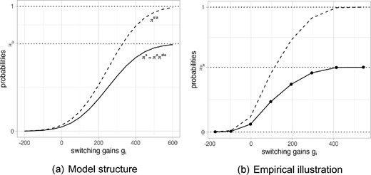
Figure 4(a) shows these probabilities for a hypothetical example. The dashed line is the conditional probability |$\pi ^{s|a}(g_i)$|, that is, the c.d.f. of switching costs. The attention probability |$\pi ^a_i$| is a fixed number (in the graph, it is 0.7). According to equation (1), the overall switching probability is simply |$\pi ^s_i(g_i)=\pi ^a_i\cdot \pi ^{s|a}(g_i)$|, that is, the c.d.f. of the switching costs scaled by a factor |$\pi ^a_i$|. It converges to |$\pi ^a_i$| as |$g\rightarrow \infty$|; that is, as savings become very large, only those unaware of them do not take action.
Model structure and identification.
In the empirical application, we observe |$g_i$| and the decision to switch, so that, we can directly identify |$\pi ^s_i(g_i)$|. As a descriptive exercise, Figure 4(b) shows the average switching rates for eight groups defined by the level of gains |$g_i$| as a solid line.12 This can be considered as a very basic estimate of the function |$\pi ^s_i(g_i)$| without any sociodemographic characteristics. As expected, the switching rate clearly increases with |$g_i$|. This function converges to a number around 0.5 as |$g_i$| grows. Our theoretical considerations suggest that this can be used as an estimate of the attention probability |$\pi ^a_i$|. If 50% of the households do not pay attention, the overall switching can never exceed 50%.
Once we have an estimate of |$\pi ^s_i(g_i)$| and |$\pi ^a_i$|, we can simply use (1) to get an estimate of switching probabilities conditional on attention, and in turn the distribution of the switching costs, as
In Figure 4(b), this estimate is shown as the dashed line. It crosses 50% at around £110, which according to the model structure can be interpreted as estimated median switching costs.
To evaluate the effect of inattention on households’ choice to adopt the changeover tariff, we also estimate a restricted model where all households are assumed to pay attention, that is, the restriction |$\pi ^a_i(\boldsymbol {x}_i)=1$| is imposed on the full model. As this restricted model consists only of the choice to switch contract, it attributes all inertia to the switching costs, thus inevitably delivering larger switching costs than those estimated with the full model.
We now analyze how sociodemographic characteristics can be used to separately identify their effects on attention probabilities and switching costs. If some households have the same switching costs but different attention probabilities, then their |$\hat{\pi }^s_i(\boldsymbol {x}_i, g_i)$| curves converge to different levels |$\pi ^a_i(\boldsymbol {x}_i)$|. If they have the same attention probabilities but different switching costs, then their |$\hat{\pi }^s_i(\boldsymbol {x}_i, g_i)$| curves converge to the same levels but may be shifted left or right.
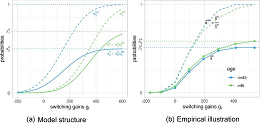
As an illustration, consider two groups of households: Group 1 has a higher attention probability but also higher average switching costs than group 2, so the overall difference in switching rates is ambiguous. Figure 5(a) depicts the switching probability of group 1 in green and of group 2 in blue. While the switching costs distribution is shifted to the left for group 2, it is scaled by a lower attention probability to arrive at the overall switching curve |$\pi ^s_2(g_i)$|. As a result, its shape differs, which then helps us to separately identify the two sources of inertia.
Identification of sociodemographic characteristics.
Figure 5(b) shows an empirical example with two groups defined by the age of contract holders. This simple analysis is just for illustrative purposes since, at this point, we do not account for any other covariates. In this case, switching converges to a lower number (implying lower attention) for the youngest group, while more senior households are more attentive. When we use these results on attention to identify the distribution of switching costs (the dashed lines), the differences are less obvious. The |$\hat{\pi }^{s|a}_i(g_i)$| curves overlap for gains below £150 and then the curve of the youngest households shifts to the left, thus suggesting lower switching costs. As mentioned, this is just an illustration, and we now move to explaining how we estimate our comprehensive model.
3.2. Specification and Estimation
As explained in Section 3.1, the main structure of our switching model is
where |$\pi ^s_i$| is the overall switching probability, |$\pi ^a_i$| is the attention probability, and |$\pi ^{s|a}_i$| is the switching probability conditional on paying attention which is driven by switching costs.
We write the attention probability similar to a simple probit model
where |$\Phi$| denotes the standard normal c.d.f. Obviously, we cannot estimate this model directly since we do not observe attention. This specification is chosen for convenience but could easily be replaced by other specifications.
Once households pay attention and know their potential gains from switching, they compare these gains with their switching costs and make the phone call if the net gain is positive. For convenience and ease of interpretation, we make a parametric assumption that the unknown switching costs are normally distributed, conditional on the household characteristics |$\boldsymbol {x}_i$|:
where the household characteristics |$\boldsymbol {x}_i$| that shift the mean switching costs can be the same as the determinants of attention. Conditional on characteristics |$\boldsymbol {x}_i$| and the gains |$g_i$|, the individual probability of switching given attention is
This is again similar to a probit model, but switching is not determined by whether unit-free utility is positive. Instead, households switch whenever the gains exceed the switching costs. Since we directly observe the switching gains |$g_i$|, we can explicitly estimate switching costs in pounds sterling as well.
Putting everything together, we have
We estimate the fully parametric model using maximum likelihood. The likelihood contribution of each household i is simply
The econometric model described above does not consider the timing of the decision, in particular the fact that households can switch to the changeover tariff at any point during the first 2 years since the change of contract. To explore the role of timing, we present results from a sequential model in Section 5, which distinguishes early and late switchers.
4. Variables and Descriptives
The institutional framework of the changeover tariff suggests that customers should not easily disregard the information they receive and they should also not find it too difficult to process and act upon such information. In order to understand what socio-economic characteristics make it more likely that a customer takes advantage of the changeover tariff, we construct a rich dataset by combining billing data and customers’ information provided by SW with data on income, education, and ethnicity at Output Areas (OA) level from the Office for National Statistics (ONS). OA is the lowest geographical level at which census estimates are provided. These were built from clusters of adjacent unit postcodes and, in 2011, had an average population of 309.13
The dataset we use to estimate our empirical model includes 225,961 customers who, by October 2015, have had a metered installed for the first time on their properties and have received at least four bills under the new tariff. Recall that after four bills (i.e. 2 years after switching contract), all customers, including those who applied for the changeover tariff, pay the normal metered bill. This sample includes 81,815 households with positive gains from adopting the changeover tariff over 2 years, and 144,146 households whose changeover bill is instead higher than the normal metered bill. While the latter are better-off under the new metered contract, our records show that 1,162 of these 144,146 customers decide to switch tariff, the vast majority because they have initial positive gains at the time they adopt the changeover tariff, but overall negative gains over the 2-year period.
Figure 6 shows the distribution of gains for the 225,961 households, distinguishing between the 24,175 households who switched to the changeover tariff and the 201,786 households who did not, resulting in a switching rate just above 10% (=24,175/225,961) for the whole sample and 28% (=(24,175−1,162)/81,815) for those with positive gains. Some interesting patterns emerge from Figure 6. First, while the great majority of households that did not switch had either negative gains or gains lower than £50, there is also a large portion of customers that would have obtained non-trivial savings. Indeed, among the 58,802 “no changeover” households with positive gains, the average savings over 2 years are £121.5 (median £83), an amount that for many families should be enough to compensate the hassle of making a phone call to the water utility. Not surprisingly, the average gain of the 24,175 customers who did call is much higher, at £198.6 (median £167), thus confirming that financial gains increase the probability of calling. Second, even for very high gains (above £300), the number of customers who do not switch contract is similar to the number who do switch. This is indicative that attention plays a key role in explaining customers’ inertia.
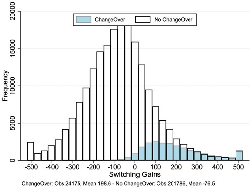
Distribution of gains/losses.The figure plots the distribution of gains/losses over 2 years for households who applied for the changeover tariff and those who did not. We windsorized the distribution below -£500 and above £500.
Table 1 reports descriptive statistics of the variables used in our empirical model, for households that switch to the changeover tariff on the left, and those that do not switch on the right. The average unmetered bills are £203 for changeover customers and £225 for the other customers. Considering that the unmetered bills do not change much over time, these two groups of households would have paid on average, around £800 and £900 over 2 years, respectively. The unmetered bill is the only information about cost of water households may be familiar with. Ceteris paribus, customers with a high unmetered bill should pay less attention to the information received as they are less likely to experience an increase in their bill due to metering. At the same time, unmetered bill is correlated with households’ wealth and other geo-social factors, which may affect switching costs. The variable is then included in both segments of equation (5).
Summary statistics.
| Changeover | No changeover | |||||
|---|---|---|---|---|---|---|
| Variables | Mean | Median | Standard deviation | Mean | Median | Standard deviation |
| SW data | ||||||
| Changeover gains|${\rm ^a}$| | 198.60 | 167 | 166.53 | -76.47 | -77 | 177.13 |
| Unmetered bill|${\rm ^b}$| | 203.44 | 202.22 | 58.80 | 225.10 | 222.56 | 77.17 |
| Occupants|${\rm ^c}$| | 3.62 | 4 | 1.12 | 2.41 | 2 | 1.15 |
| Age|${\rm ^d}$| | 49.49 | 49 | 12.06 | 55.38 | 55 | 15.32 |
| ONS data | ||||||
| Education score|${\rm ^e}$| | -0.258 | -0.219 | 0.178 | -0.236 | -0.194 | 0.173 |
| Income score|${\rm ^f}$| | -0.142 | -0.120 | 0.086 | -0.126 | -0.110 | 0.082 |
| Homogeneity|${\rm ^g}$| | 0.788 | 0.835 | 0.158 | 0.809 | 0.850 | 0.143 |
| Social rented|${\rm ^h}$| | 0.159 | 0.146 | 0.091 | 0.156 | 0.142 | 0.096 |
Note: Statistics for the 24,175 changeover households and 201,786 no changeover households.
|${\rm a.}\,$| The amount of money the customers can save by using the changeover plan.
|${\rm b.}\,$| The amount of money the customers used to pay before a meter was installed.
|${\rm c.}\,$| The number of people living in that household.
|${\rm d.}\,$| Age of the contract holder.
|${\rm e.}\,$| The extent of deprivation in terms of education, skills, and training in an output area.
|${\rm f.}\,$| The extent of deprivation in terms of low income in an output area.
|${\rm g.}\,$| Similar ethnical groups in an output area.
|${\rm h.}\,$| The proportion of social housing in the area.
Not surprisingly, the number of occupants is larger in the group of households that adopt the changeover tariff: on average, 3.6 occupants versus 2.4 occupants for the other group. Most of the households consist of two or three people, with a maximum value capped at six when there are more than six people living at the same address. As the number of households in this group is rather small, in the empirical analysis we will group households with five and six occupants together. As for the unmetered bill, we anticipate that the size of the household can affect the probability of switching by affecting both the probability of paying attention, as more numerous households may expect a larger shock due to metering, and the costs of considering and carrying out the switch of contract.
The mean age of the contract holder in the changeover group is 49:6 years younger than the contract holder in the other group.14 In the empirical analysis, we divide households in three age groups: below 35, between 35 and 65, and above 65.
Looking at the variables retrieved from ONS, the education score measures the extent of deprivation in terms of education, skills, and training in an area,15 while the income score refers to the proportion of the population in an area experiencing deprivation related to low income.16 Education and income score are calculated at the OA level and, originally, they are between 0 and 1, with an higher index indicating more deprived areas. We transform these variables by multiplying them by -1, so that a lower index is associated with more deprivation. The descriptive statistics reported in Table 1 show that households in the changeover group live in areas with higher levels of deprivation in both education and income.17 In the econometric analysis, we discretize income and education scores splitting the distribution in three groups, group 1 (Low) up to the first quartile, group 2 (Medium) between the first and third quartile, and group 3 (High) above the third quartile.
Another variable we retrieve from the ONS is the percentage of social rented housing in the area, Social Rented. These are houses provided at an affordable rent by housing associations (not-for-profit organizations that own, let, and manage rented housing) or a local council. This variable complements the information about wealth and income that is provided by the unmetered bill (because, as said, this is related to the rateable value of the house) and to the income index at OA.
The last variable in Table 1, Homogeneity, is the Herfindahl–Hirschman Index of concentration of different ethnicities in an OA. It is computed as the sum of squares of the percentage of seven different groups: White British, other White, Black, Pakistani, Indian, other Asian, and other ethnic groups. Note that White British represents on average 87% (median: 90%) of the population in the areas affected by the universal metering program, with Pakistanis, Indians, and Black people representing the most relevant minorities. Accordingly, a low level of homogeneity is indicative of a higher presence of these ethnic groups in an OA. Homogeneity is included in our empirical specifications to capture cultural differences that can affect attention and switching costs. Specifically, higher homogeneity may affect attention through word-of-mouth recommendations among neighbors. The numbers in Table 1 indicate that there are no major differences in Homogeneity between the two groups.
Finally, our specification includes a dummy indicating the quarter of the year when households receive their first bill. These quarterly dummies control for seasonality in consumption which can affect the probability of switching if households factor in that future consumption (and, in turn, financial gains from switching) may not be the same as past consumption used to compute the savings shown in the pie charts.18
5. Results
In this Section, we first present the results for the full model described in equation (1) vis-à-vis a restricted model that assumes that switching costs are the only determinant of consumers’ inaction. Then, in Section 5.2, we investigate how the results of the full model may change when taking into account that customers can take the decision to switch tariff over a period of 2 years.
5.1. Main Results
Recall that the probability of adopting the changeover tariff in the full model is defined as
where, conditional on individuals paying attention, the term |$\pi ^{s|a}_i(\boldsymbol {x}_i, g_i)$| reflects the comparison between the realized gains from adopting the changeover tariff over the 2 years and the latent switching costs.
To better gauge the importance of allowing for inattention to explain consumers’ inertia, we also specify a simpler model where we restrict the attention probability to be |$\pi ^a_i(\boldsymbol {x}_i)=1$| for everybody. This restricted model therefore explains the observed inertia of households who would profit from changing contract with switching costs.
Table 2 presents the average estimated values of the probability of switching for the restricted model and the full model, considering the whole sample (top panel) and households with positive gains (bottom panel). Because the full model explains a large share of non-switching with inattention, attentive individuals have a much higher probability to switch than in the restricted model: 21.7% versus 10.4% for the whole sample and 55.8% versus 24.4% for households with positive gains. This large difference in the probability of switching implies vastly different estimated switching costs, as shown in Figure 7. The restricted model estimates median switching costs above £400 which seems unrealistically high, considering the low effort required to adopt the changeover tariff. The full model estimates this cost at a much more reasonable figure of around £100. Furthermore, Figure 7 shows that, in the restricted model, all households are found to have switching costs well above £200, with estimates above £600 for some of them. This confirms that switching costs would need to be unreasonably large to explain the low switching rates we observe.
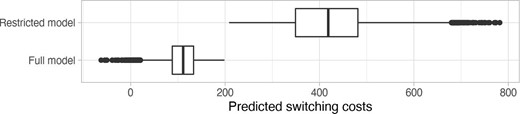
Distribution of switching costs.
Probability of switching.
| All households | Restricted model | Full model |
|---|---|---|
| Switching |$\pi ^s_i(\boldsymbol {x}_i, g_i; \boldsymbol{\beta }, \boldsymbol{\gamma }, \sigma )$| | 0.104 | 0.107 |
| Attention |$\pi ^a_i(\boldsymbol {x}_i)$| | 1.000 | 0.475 |
| Switching if attentive |$\pi ^{s\vert a}_i(\boldsymbol {x}_i, g_i)$| | 0.104 | 0.217 |
| Households with positive gains | Restricted model | Full model |
| Switching |$\pi ^s_i(\boldsymbol {x}_i, g_i; \boldsymbol{\beta }, \boldsymbol{\gamma }, \sigma )$| | 0.244 | 0.275 |
| Attention |$\pi ^a_i(\boldsymbol {x}_i)$| | 1.000 | 0.495 |
| Switching if attentive |$\pi ^{s\vert a}_i(\boldsymbol {x}_i, g_i)$| | 0.244 | 0.558 |
We now look at the effects of individual characteristics and socio-economic indicators at OA level on the probability of adopting the changeover tariff. Table 3 shows the results for the restricted model in column (1) and the full model in column (2). Recall that the coefficients on the variables in the top part of the table can be interpreted in terms of pounds sterling. The magnitude of the coefficients for the attention stage in the bottom part of the table does not have a direct economic interpretation. Therefore, in Table 4, we report the implied average partial effects (in percentage points) of the households’ characteristics on the overall switching probability as well as the probability to pay attention and the probability to switch given attention.
Attention and switching costs.
| Model 1 | Model 2 | |
|---|---|---|
| Switching costs: | ||
| Intercept | |$496.19 \,\, (9.02)^{***}$| | |$168.48 \,\, (7.22)^{***}$| |
| Two occupants | |$-126.93 \,\, (7.15)^{***}$| | |$-27.64 \,\, (5.49)^{***}$| |
| Three occupants | |$-212.88 \,\, (7.21)^{***}$| | |$-55.27 \,\, (5.61)^{***}$| |
| Four occupants | |$-263.98 \,\, (7.61)^{***}$| | |$-72.77 \,\, (5.96)^{***}$| |
| More than five occupants | |$-230.22 \,\, (7.88)^{***}$| | |$-66.79 \,\, (6.00)^{***}$| |
| Age 35–65 | |$-34.04 \,\, (3.56)^{***}$| | |$-1.39 \,\, (3.29)$| |
| Age |$>$|65 | |$8.64 \,\, (4.42)$| | |$-4.65 \,\, (3.89)$| |
| Education medium | |$4.13 \,\, (3.02)$| | |$7.54 \,\, (2.62)^{**}$| |
| Education high | |$0.72 \,\, (4.05)$| | |$8.77 \,\, (3.39)^{**}$| |
| Income medium | |$-6.60 \,\, (2.84)^{*}$| | |$8.28 \,\, (2.42)^{***}$| |
| Income high | |$13.02 \,\, (5.33)^{*}$| | |$9.67 \,\, (4.25)^{*}$| |
| Social rented | |$105.88 \,\, (14.52)^{***}$| | |$28.44 \,\, (12.19)^{*}$| |
| Homogeneity | |$-3.65 \,\, (2.62)$| | |$15.94 \,\, (2.14)^{***}$| |
| Unmetered bill | |$34.55 \,\, (2.14)^{***}$| | |$-15.80 \,\, (1.60)^{***}$| |
| Quarter 2 | |$8.33 \,\, (3.13)^{**}$| | |$-3.17 \,\, (2.60)$| |
| Quarter 3 | |$-8.09 \,\, (3.10)^{**}$| | |$-13.06 \,\, (2.57)^{***}$| |
| Quarter 4 | |$9.37 \,\, (3.76)^{*}$| | |$-4.98 \,\, (3.18)$| |
| Standard deviation |$\sigma$| | |$272.43 \,\, (1.75)^{***}$| | |$97.50 \,\, (0.99)^{***}$| |
| Attention probability: | ||
| Intercept | |$0.13 \,\, (0.09)$| | |
| Two occupants | |$0.03 \,\, (0.09)$| | |
| Three occupants | |$-0.05 \,\, (0.08)$| | |
| Four occupants | |$-0.01 \,\, (0.08)$| | |
| More than five occupants | |$0.09 \,\, (0.08)$| | |
| Age 35–65 | |$0.20 \,\, (0.03)^{***}$| | |
| Age |$>$|65 | |$0.07 \,\, (0.03)^{*}$| | |
| Education medium | |$0.06 \,\, (0.02)^{**}$| | |
| Education high | |$0.09 \,\, (0.03)^{**}$| | |
| Income medium | |$0.10 \,\, (0.02)^{***}$| | |
| Income high | |$0.05 \,\, (0.04)$| | |
| Social rented | |$-0.24 \,\, (0.10)^{*}$| | |
| Homogeneity | |$0.13 \,\, (0.02)^{***}$| | |
| Unmetered bill | |$-0.20 \,\, (0.02)^{***}$| | |
| Quarter 2 | |$-0.05 \,\, (0.02)^{*}$| | |
| Quarter 3 | |$-0.01 \,\, (0.02)$| | |
| Quarter 4 | |$-0.08 \,\, (0.03)^{**}$| | |
| Log likelihood | |$-52,\!328.08$| | |$-48,\!795.59$| |
Notes: Homogeneity is the Herfindahl–Hirschman Index of concentration of different ethnicities in an output area. Social rented is the percentage of social rented housing in the same area. Unmetered bill is measured in £100. Quarter refers to the quarter of the year when the households receive their first bill. Standard deviation refers to the unobserved heterogeneity of the switching costs. |$^{*}p<0.05$|; |$^{**}p<0.01$|; and |$^{***}p<0.001$|.
Probability of switching and paying attention.
| Pr(switching) | Pr(attention) | Pr(switching|attention) | |
|---|---|---|---|
| Average probability | 10.66 | 47.50 | 21.71 |
| Two occupants | 1.74 | 1.14 | 3.13 |
| Three occupants | 2.82 | -2.04 | 6.73 |
| Four occupants | 4.43 | -0.33 | 9.26 |
| More than five occupants | 4.97 | 3.63 | 8.38 |
| Age 35–65 | 1.74 | 7.64 | 0.17 |
| Age |$>$|65 | 0.84 | 2.65 | 0.58 |
| Education medium | 0.03 | 2.22 | -0.95 |
| Education high | 0.23 | 3.47 | -1.10 |
| Income medium | 0.38 | 4.00 | -1.04 |
| Income high | -0.17 | 1.82 | -1.21 |
| Social rented | -3.33 | -9.17 | -3.34 |
| Homogeneity | 0.13 | 5.16 | -1.98 |
| Unmetered bill | -0.83 | -7.61 | 2.04 |
A number of interesting results emerge from these two tables. First, both models show that an increase in the number of occupants is associated with a reduction in switching costs (with a minor change for the group of five or more occupants), a result that can be explained by the fact that there may be some specialization and division of tasks within large households. However, the restricted model produces estimates of the switching costs that are four to five times higher than those delivered by the full model. These numbers exemplify that, when including the attention stage, differences in switching rates between small and large households do not need to be explained by extremely large difference in switching costs, as in the restricted model.
Second, the restricted model suggests that switching costs are not different across areas with low or high education scores, and they do not show a clear pattern as we move from areas with low to areas with high income scores. However, a different picture emerges from the full model: Households in less deprived areas are more likely to pay attention but, conditional on paying attention, are found to have higher switching costs. Specifically, Table 4 shows that, compared with households in low income and low education neighborhoods (the reference group) with identical other characteristics, households in medium or high education income neighborhoods are more likely to pay attention by 2.2 and 3.4 percentage points, respectively. Similarly, households in medium and high income neighborhoods are more likely to pay attention by 4 and 1.8 percentage points, respectively. Moreover, Table 4 shows that, conditional on paying attention, households living in areas with higher levels of income and education are less likely to switch compared with the reference group. This is consistent with the idea that households with higher education and income may find it easier to understand the information but they may also have higher opportunity costs in acting upon such information.
Third, the full model estimates higher switching costs and lower attention in areas with a high proportion of social rented housing. More precisely, the numbers in Table 4 indicate that a one standard deviation increase in the proportion of social rented housing decreases the probability of paying attention by around 1 percentage point (=-9.17 * 0.091) and, conditional on paying attention, is associated with a decrease in probability of switching by 0.3 percentage point (=-3.34 * 0.091). This finding suggests that the changeover program is likely to exacerbate inequalities among households.
Fourth, the restricted model estimates switching costs for contract holders in their prime age (between 35 and 65 years old) to be £34 lower than contract holders below 35 (the reference group). Interestingly, in the full model, we observe that the prime age group is characterized by a higher probability of paying attention but no differences in switching costs. In other words, a higher switching rate among prime age group is not due to lower switching costs (as suggested by the restricted model) but to the fact that households in this group are more likely to pay attention by 7.64 percentage points.
Fifth, Tables 3 and 4 show the estimated effect of the unmetered bill measured in £100. An increase of £100 in the unmetered bill is associated with a decrease in switching costs by £15.8, which translates into higher switching probability of attentive households by 2 percentage points. At the same time, the attention probability decreases by 7.6 percentage points, entailing a decrease in overall switching probability by 0.8 percentage points. This is consistent with the idea that households who are used to pay a high bill may be less worried about the financial implications of metering, and therefore pay less attention to the whole process.
The effects of racial homogeneity is also noteworthy. The full model shows that the higher switching rate in areas with high concentration of White Caucasians are driven by higher level of attention (5.16 percentage points) while, conditional on paying attention, the probability of switching is actually lower (-1.98 percentage points). Two reasons can explain this result. First, higher homogeneity may facilitate social interaction and word-of-mouth diffusion of information, triggering a higher alert among households affected (e.g. neighbors mentioning the savings they realized by adopting the alternative tariff). Second, areas with lower homogeneity may be characterized by a higher share of non-native speakers, who may find it more difficult to fully engage with the information material provided by the water company.
Finally, the standard deviation |$\sigma$| measures the unobserved heterogeneity of the switching costs, that is, the standard deviation of the switching costs conditional on the household characteristics (see equation (3)).
To provide some intuition on the model mechanics and results, Figure 8 plots switching gains against estimated switching probabilities for the restricted model without the attention stage, while Figure 9 depicts the relevant aspects of the full model. In both cases, the black points represent the estimated switching probabilities. In the restricted model, switching costs are the only explanation of inaction. Therefore, the estimated switching cost distributions depicted by the red lines are very high. The minimum and maximum distributions refer to the households with the highest and the lowest predicted switching costs. For the average household (in terms of the switching costs explained by the regressors), median switching costs are above £400.
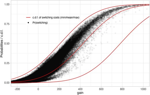
Restricted model: switching probabilities and costs.

Full model: attention probabilities, switching probabilities, and costs.
In the full model (Figure 9), the estimated switching probabilities are not forced to converge to 1 as gains go to infinity. Instead, they are allowed to converge to different values, which are then interpreted as the attention probabilities. As noted before, attention probabilities are slightly below 0.5 on average, but they vary quite a bit depending on the values of the explanatory variables, as depicted by the dashed green lines. The switching costs, shown in blue, are identified from the switching probabilities conditional on attention. The c.d.f.s of the minimum, maximum, and mean switching costs are shown in red. They are much lower that in the restricted model since the low switching rates even at high gains do not have to be explained by switching costs.
5.2. Sequential-Response Model
The results above demonstrate that our full model not only delivers more reasonable estimates of switching costs compared with a model that assumes that customers are fully informed, but provides also valuable insights on how attention and switching costs vary among households with different socio-economic characteristics. However, one limitation of our empirical framework is that it does not consider when the switching took place. In this section, we explore how switching costs and attention differ between the customers that adopt the changeover tariff before the second bill (“early-switch” group) and those that call after receiving the second bill (“late-switch” group).19
We follow a classical approach (Amemiya 1975) called a sequential discrete choice model (see also Maddala (1983), Section 2.14). We start by specifying a model with the same structure as before, but restrict the outcome “switching” to those who switched early, that is, those who call before the second bill. The results of this model are shown in the first column of Table 6. We then study the remaining households who did not switch early and estimate a model for late switching (given no early switching). The overall probability of late switching can then be reconstructed as Pr(late switching) = Pr(no early switching) |$\times$|Pr(late switching | no early switching). The results of this model are shown in the second column of Table 6.
Probability of switching—time of adoption.
| Overall | |||
|---|---|---|---|
| Households with positive gains | (Table 2) | Early switch | Late switch |
| Switching |$\pi ^s_i(\boldsymbol {x}_i, g_i; \boldsymbol{\beta }, \boldsymbol{\gamma }, \sigma )$| | 0.275 | 0.218 | 0.071 |
| Attention |$\pi ^a_i(\boldsymbol {x}_i)$| | 0.495 | 0.382 | 0.229 |
| Switching if attentive |$\pi ^{s\vert a}_i(\boldsymbol {x}_i, g_i)$| | 0.558 | 0.576 | 0.316 |
Attention and switching costs—time of adoption.
| Early switch | Late switch | |
|---|---|---|
| Switching costs: | ||
| Intercept | |$123.93 \,\, (7.20)^{***}$| | |$249.79 \,\, (16.70)^{***}$| |
| Two occupants | |$-15.46 \,\, (5.61)^{**}$| | |$-10.81 \,\, (12.63)$| |
| Three occupants | |$-25.46 \,\, (5.68)^{***}$| | |$-38.38 \,\, (12.80)^{**}$| |
| Four occupants | |$-34.50 \,\, (5.96)^{***}$| | |$-42.33 \,\, (13.52)^{**}$| |
| More than five occupants | |$-27.82 \,\, (6.00)^{***}$| | |$-47.62 \,\, (13.50)^{***}$| |
| Age 35–65 | |$2.32 \,\, (3.39)$| | |$16.53 \,\, (7.13)^{*}$| |
| Age |$>$|65 | |$0.69 \,\, (3.93)$| | |$14.40 \,\, (9.11)$| |
| Education medium | |$3.50 \,\, (2.62)$| | |$11.84 \,\, (6.12)$| |
| Education high | |$8.18 \,\, (3.36)^{*}$| | |$10.83 \,\, (8.27)$| |
| Income medium | |$9.38 \,\, (2.42)^{***}$| | |$17.09 \,\, (5.56)^{**}$| |
| Income high | |$4.38 \,\, (4.17)$| | |$7.47 \,\, (10.59)$| |
| Social rented | |$18.16 \,\, (12.29)$| | |$-4.00 \,\, (29.78)$| |
| Homogeneity | |$10.12 \,\, (2.11)^{***}$| | |$21.50 \,\, (5.18)^{***}$| |
| Unmetered bill | |$-8.87 \,\, (1.45)^{***}$| | |$-33.98 \,\, (3.85)^{***}$| |
| Gains change |$\delta$| | |$0.03 \,\, (0.01)^{*}$| | |$0.72 \,\, (0.02)^{***}$| |
| Quarter 2 | |$-1.20 \,\, (2.69)$| | |$6.24 \,\, (5.85)$| |
| Quarter 3 | |$-5.99 \,\, (2.56)^{*}$| | |$0.55 \,\, (6.43)$| |
| Quarter 4 | |$5.10 \,\, (2.99)$| | |$-17.26 \,\, (9.07)$| |
| Standard deviation |$\sigma$| | |$79.73 \,\, (0.76)^{***}$| | |$119.45 \,\, (2.53)^{***}$| |
| Attention probability: | ||
| Intercept | |$-0.52 \,\, (0.08)^{***}$| | |$-0.22 \,\, (0.15)$| |
| Two occupants | |$0.20 \,\, (0.07)^{**}$| | |$-0.21 \,\, (0.14)$| |
| Three occupants | |$0.21 \,\, (0.07)^{**}$| | |$-0.38 \,\, (0.14)^{**}$| |
| Four occupants | |$0.20 \,\, (0.07)^{**}$| | |$-0.31 \,\, (0.14)^{*}$| |
| More than five occupants | |$0.22 \,\, (0.07)^{**}$| | |$-0.26 \,\, (0.13)$| |
| Age 35–65 | |$0.25 \,\, (0.02)^{***}$| | |$0.04 \,\, (0.04)$| |
| Age |$>$|65 | |$0.15 \,\, (0.03)^{***}$| | |$-0.11 \,\, (0.06)$| |
| Education medium | |$0.07 \,\, (0.02)^{***}$| | |$-0.02 \,\, (0.04)$| |
| Education high | |$0.16 \,\, (0.03)^{***}$| | |$-0.08 \,\, (0.05)$| |
| Income medium | |$0.16 \,\, (0.02)^{***}$| | |$-0.04 \,\, (0.04)$| |
| Income high | |$0.12 \,\, (0.03)^{***}$| | |$-0.17 \,\, (0.07)^{**}$| |
| Social rented | |$-0.30 \,\, (0.10)^{**}$| | |$-0.19 \,\, (0.19)$| |
| Homogeneity | |$0.08 \,\, (0.02)^{***}$| | |$0.18 \,\, (0.04)^{***}$| |
| Unmetered bill | |$-0.19 \,\, (0.01)^{***}$| | |$-0.03 \,\, (0.03)$| |
| Gains change | |$0.00 \,\, (0.00)$| | |$0.00 \,\, (0.00)$| |
| Quarter 2 | |$-0.04 \,\, (0.02)^{*}$| | |$-0.05 \,\, (0.04)$| |
| Quarter 3 | |$0.08 \,\, (0.02)^{***}$| | |$-0.26 \,\, (0.04)^{***}$| |
| Quarter 4 | |$0.12 \,\, (0.02)^{***}$| | |$-0.59 \,\, (0.05)^{***}$| |
| Log likelihood | |$-42,\!191.59$| | |$-16,\!230.94$| |
Note: Homogeneity is the Herfindahl–Hirschman Index of concentration of different ethnicities in an output area. Social rented is the percentage of social rented housing in the same area. Unmetered bill is measured in £100. Gains change is the difference between the actual overall gains over the 2 years and the gains indicated in the first bill. Quarter refers to the quarter of the year when the households receive their first bill. Standard deviation refers to the unobserved heterogeneity of the switching costs. |$^{*}p<0.05$|; |$^{**}p<0.01$|; and |$^{***}p<0.001$|.
We note that the results for the late switching are conditioning on not having switched early. This means that these customers are likely to be a selected subgroup of households, and, in turn, the results cannot be interpreted as pertaining to the general population. Since we do not know the reason why households did not switch early (i.e. they did not pay attention or they have high switching costs), we have no way to control for correlations between early stage and late stage, and so we are unable to infer how the general population would have behaved in the late stage.
Of the 24,174 customers that adopt the changeover tariff, 18,953 of them are classified as “Early switch” and 5,222 are part of the “Late switch” group. The number of observations used to estimate the coefficients in columns (1) and (2) of Table 6 is respectively, 225,961 (the same as Table 3) and 207,008. The lower number of observation is due to the fact that, in the second column, we compare the characteristics of the 5,222 households who call late to the 201,786 households who do not switch tariff, but we drop the 18,953 customers that have already adopted the changeover tariff by calling early.
Table 5 shows that, for households with positive savings from switching, we estimate an average switching probabilities of 21.8% in the early stage. Among the (100–21.8=) 78.2% of households who do not switch early, the model for late switching implies average switching probabilities of 7.1%. This corresponds to 78.2% |$\times$| 7.1% = 5.6% of all households. The overall switching probability of 21.8 + 5.6 = 27.4% is consistent with the overall switching share, reported again in the first column of Table 5 for convenience. The implied probability to pay attention is only 38.2% in the early stage, which explains the difference between overall switching and early switching. On the contrary, the estimated switching costs and the implied conditional switching probabilities given attention are quite similar (55.8% vs. 57.6%). For the late switch, the average probability to pay attention is 22.9% and, if individuals do pay attention, the conditional switching probability is merely 31.68%. The difference between this number and the 57.6% for early switching can be explained by selection: by only looking at individuals who didn’t switch early, we select a sample with higher average switching costs.
To evaluate the role of new information gathered between the first bill and subsequent bills, we separate the financial gains |$g_i$| into two parts. One is the savings indicated in the first bill, extended over the 2 years period. The other is the ex-post difference of the actual overall gains and this earlier prediction. More formally, “overall gains” |$g_i$| = “gains implied by first bill” |$g_i^1$| + “gains change”|$g_i^\Delta$|.20 One of our identifying assumptions is that, conditional on observables like the unmetered bill and the number of occupants, the gains do not affect attention. With this separation, we can maintain this assumption for early implied gains while adding |$g_i^\Delta$| as a predictor into the attention stage. Reassuringly, we do not find any significant predictive power as shown in the lower part of Table 6.
The switching decision of attentive households depends on a comparison between gains and switching costs. If we allow the different parts of the gains to be taken into account with a different weight, we can rewrite equation (4) as
The new coefficient |$\delta$| would be equal to 1 if households took the updated information fully into account. As shown in the upper part of Table 6, we find that the parameter is small but significantly different from 0 for early switching, indicating that a small group of households understand the problem well enough to be able to predict future water consumption changes and their effect on their optimal tariff choice. The coefficient is quite large (0.72) for late switching. This suggests that most of the small group of customers who pay attention in the late decision round correctly take into account changes in water consumption and, in turn, in the actual savings from adopting the changeover tariff.
The other coefficients in the early switching results are qualitatively similar to the main results on overall switching. One notable exception is that the coefficients on occupants in the attention stage are positive and significantly different from 0, but almost exactly the same for two, three, five, and more than five occupants. This implies that single households ceteris paribus pay less attention early than larger households. As number of occupants is the most important predictor of consumption and, in turn, potential savings, the fact that coefficients are the same across all the groups of occupiers suggests that the probability of paying attention is not driven by expected savings. The coefficients for late switching are considerably different. But, since they pertain to a different and selected sub-population, they are more difficult to interpret. Single households appear to catch up somewhat in terms of attention since the coefficients of the number of occupants are negative and at least in part significantly different from 0. This explains why we do not find any significant differences in our main results on overall switching.
6. Conclusion
This paper shows how consumers fail to choose the most convenient between two water tariffs, in a setting where the choice should be salient and where other mechanisms that have been proposed in the literature to explain inertia, like status quo as reference point or “sticking with what you know”, do not play a role. We disentangle the role of inattention and switching costs, showing how the former plays a key role, and explore heterogeneity along dimensions like income and education.
Our findings have important policy implication. Consumer choice is a centrepiece of current market regulation policies promoting an increase in competition among suppliers. For instance, to control energy costs, the recently adopted EU energy policy framework Clean Energy for All Europeans requires energy suppliers to provide free access to at least one energy comparison tool and clearer information in household bills.21 As underlined in the literature (Waterson 2003), the impact of such measures is greatly diminished if consumers display a high degree of passivity, as documented in this paper. Our finding that low income/low education is associated with lower attention also raises distributional issues, as people from low socio-economic background appear to be the least likely to benefit from increased choice.
Similarly, the British energy regulator, Ofgem, has launched a program to address low levels of consumer engagement, testing measures “to encourage consumer engagement, promote competition and innovation in the retail energy market”.22 These measures include a so-called Cheaper Market Offer Communication, contacting customers with better tariff offers by post, or Collective Switch, where, similarly to our setting, customers on a default energy tariff received letters showing personalized savings if they switched from their current deal to an exclusive tariff. All these measures can be effective, but, crucially, require consumers to pay attention, something that, as we show, cannot be taken for granted. It would therefore be important for regulators to add to their toolbox measures aimed directly at increasing attention. For instance, there is a literature showing the importance of word-of-mouth communications, where information is conveyed through personal networks (see, for instance, Duflo and Saez 2003; Banerjee et al. 2013). There could be incentives to encourage engaged consumers to reach out to disengaged ones, along the lines of incentives provided by firms looking for employees (Burks et al. 2015) or in marketing (Aral and Walker 2011; Bapna and Umyarov 2015; Wolters, Schulze, and Gedenk 2020). This would have the advantage of leveraging on trust and direct experience by peers, and could be a promising venue to boost attention. Alternatively, in some contexts, individuals could be forced to make an active choice (see Heiss et al. 2021). For instance, in the context we study, customers could have been required to choose between metered and changeover tariffs, without providing a default. This would have entailed, however, considerable paperwork and possible disruptions in water supply if people failed anyway to comply.
In contexts in which it is not feasible to reach 100% attention, there is room for policy initiatives aimed at protecting consumers with low propensity to pay attention to tariffs and switch to the most convenient ones. An example of such a policy is the UK Domestic Gas and Electricity (Tariff Cap) Act that requires the energy regulator to design and implement a temporary cap on standard variable tariffs and fixed term default tariffs, entered into force on 1 January 2019 until 2023. As explained in the Ofgem website,23 “[t]hese tariffs are an energy supplier’s basic offer, and tend to apply if you have not shopped around for a better deal. They are typically poorer value and more expensive than a non-default, fixed-term contract deal, which you can choose to switch to. You will often need to renew fixed-term contracts after a year or more. If you have never switched, or not switched for a long time, you are likely to be on one of these tariffs. Over half of all households in Great Britain are on these tariffs because they have never switched or have not done so recently”. In the context we study, it would have been feasible to automatically apply to each household the most convenient tariff. However, as explained in Section 2, this would have been more expensive and less targeted under the—ex ante reasonable but not validated by our results—assumption that lower income households were more likely to call.
Our findings of massive inertia in an environment that should be favorable to consumers taking action suggest that policy interventions should not take consumers’ attention for granted but need to be accompanied by appropriate design choices and specific measures that can raise awareness. Yet, due consideration should be given to the fact that, even after deploying such measures, a non-negligible share of the public may still not pay attention, therefore calling for measures aimed at passive consumers. This is particularly important if, as we show, the most vulnerable part of the population is the most prone to inattention.
Acknowledgments
A previous version of this paper was circulated under the title: “Water Tariff and Consumers’ Inaction”. This study was financed through an Economic and Social Research Council (ESRC) grant (ES/K01210X/1) and through the University of Southampton Strategic Research Development Fund. The authors thanks the Department of Innovation, Research, University and Museums of the Autonomous Province of Bozen/Bolzano for covering the Open Access publication costs. We would like to thank Southern Water for providing the data. Carlos Pineda provided excellent research assistance. We would like to thank the editor and anonymous referees, as well as numerous colleagues and participants at seminars and conferences for useful discussions. Tonin is affiliated to IZA, CESifo, and Dondena Centre for Research on Social Dynamics and Public Policy.
Notes
The editor in charge of this paper was Pierre Dubois.
Footnotes
Also regarding water, Wichman (2017) studies information provision through a natural experiment and demonstrates how increasing bill frequency leads to higher water consumption. Szabó and Ujhelyi (2015) implement a randomized water education campaign to reduce water non-payment in South Africa and show the importance of reciprocity.
This is related to the literature on consumer search heterogeneity. Byrne and Martin (2021) provide a recent overview showing how there is an inverse-U-shape relationship between consumers’ willingness to search and their income, with both high- and low-income households searching less.
This is in line with the findings by Kiser (2002), who uses survey data on deposit account holders and shows that “[s]witching costs appear more severe for households with high income or education and for households with very low income or minority ethnicity”.
In particular, water tariffs are regulated through a price-cap regime implemented by Ofwat over a 5-year regulatory period. The volume tariff corresponds to the (expected) average costs of water service that will be incurred by regional utilities to supply and treat water and to maintain and improve the water supply and drainage system (e.g. replacement of pipes to reduce leakage and spillages from sewage into rivers) over the next regulatory period.
Ofwat response to freedom of information request FOI 202110117 of 12 November 2021.
The document reads as follows: “All our customers will be given the opportunity to choose a ‘Changeover’ tariff for paying their water bills. This means that if your metered bill is higher than your old bill, we will reduce your bill for the first two years—and you do not have to pay the difference. This is to help you adjust to paying for your water when you are paying for what you use. Please be aware that you cannot opt for our ‘Changeover’ tariff until your meter charges start.”
In the first report by the Consumer Council for Water (CCW 2013), they write, “The survey at M1 [before meter installation, ed.] showed that a third of respondents (n=200) thought that their water bill would increase (a fifth felt it would increase by ‘a lot’); a little less than a third expected a decrease and the same number did not know what to expect” and “[t]he M1 survey showed that of the third of the sample (n=67) who expected their bill to increase, nearly half thought they might struggle to pay or would be unable to afford it while two-fifths felt that they would find it harder to pay but would manage to do so”.
Number of people in the households and unmetered bill are indeed the most important predictor of the bill shock, explaining around 90% of the variation in the difference between metered and unmetered bill. See Ornaghi and Tonin (2021) for further details.
The gains thresholds for the grouping are -£150, -£50, £50, £150, £250, £350, and £500. The horizontal axis shows the average gains and the vertical axis shows the switching rate in these groups.
For details, see: http://www.ons.gov.uk/methodology/geography/ukgeographies/.
These figures are consistent with those reported in the Labour Force Survey for England as a whole, which indicates that the median age of the household reference person in 2014 was 51 years. The reference person is the adult contributing most to the total income of the household, a concept not equivalent to the contract holder, but nevertheless informative.
It is based on a series of indicators like, for instance, the proportion of adults aged 25–54 with no or low qualifications, or the proportion of young people not staying on in school or non-advanced education above the age of 16.
It is based on a series of indicators such as adults and children in Income Support families or adults and children in income-based Jobseeker’s Allowance families.
As a term of comparison, for England as a whole, the equivalent measure of the scores are rather similar, at -0.22 (median -0.16) for the education score and at -0.15 (median -0.11) for the income score.
For instance, assume that consumption is higher during summer months and a customer receives the first bill at the end of the summer indicating high savings from adopting the changeover tariff. These savings assume for the cold season the same consumption pattern of the past summer months. This means that we may overestimate switching costs of this customer if she does not switch, when in reality she may know that the expected savings are smaller because her water consumption is lower during the cold season. We are grateful to an anonymous referee for pointing this out.
We thank an anonymous referee for suggesting this extension to our main specification.
In most cases, there is not a big change over time which is reflected in the fact that the correlation between |$g_i$| and |$g_i^1$| is 0.95.
