


Abstract
We investigate women’s fertility, labor, and marriage market responses to a health innovation that led to reductions in mortality from treatable causes, and especially large declines in child mortality. We find delayed childbearing, with lower intensive and extensive margin fertility, a decline in the chances of ever having married, increased labor force participation, and an improvement in occupational status. Our results provide the first evidence that improvements in child survival allow women to start fertility later and invest more in the labor market. We present a new theory of fertility that incorporates dynamic choices and reconciles our findings with existing models of behavior.
1. Introduction
This paper investigates fertility, labor market, and marriage market responses to sharp declines in mortality and morbidity occasioned by a medical innovation, the introduction of antibiotics in 1937 in the United States. Pneumonia was a leading cause of death among children and it was treatable by these first generation antibiotics. We find that the sharp drop in pneumonia mortality risk in infancy is associated with lower fertility at both the intensive and the extensive margins. We outline a model that can explain this, augmenting the classical quantity–quality model of fertility with a dynamic process for childbearing that takes account of women’s labor market opportunities. Women in the model choose the timing of fertility, balancing the insurance value of starting early against the option value of delay, with the option value defined on enhanced labor market prospects. We characterize how the trade-off between early and delayed fertility depends on the rate of child mortality. Consistent with the predictions of this model, we find that women delay childbearing are less likely to have ever married, more likely to work and to have higher occupational scores (a measure of the skill intensity of employment).
Ours is the first attempt to analyze, within a single framework, how child mortality may modify the timing of birth, childlessness, the number of children, labor force participation, and marriage. In contrast to previous studies that focus on one or the other, we take into account both the child quality versus quantity trade-off and the family versus career trade-off. In particular, relative to Becker and Lewis (1973) and models that build on it (e.g. Kalemli-Ozcan 2003; Soares 2005; Galor 2012; Aaronson, Lange, and Mazumder 2014), we add a third dimension to the quantity–quality trade-off, namely fertility timing, the other side of which is labor market participation. We also incorporate in the model the potential role of improvements in women’s health, although the absolute infection rate among adults was many times lower than among children.
Our key insight is that innovations that affect the relative prices of child quantity and quality may also affect the disposable time of women, leading them to delay fertility and participate in the labor market. Child mortality decline implies that women need fewer pregnancies in order to achieve their target number of children, and that the target number is likely to decline due to a reduction in the price of having a higher quality child. This encourages fertility delay, which makes it more attractive to invest in the labor market. This can have knock on effects: It becomes unnecessary to marry early and any of positive shocks to wage earnings, learning about the benefits of work, or declines in the biological ability to have children with age can shift the opportunity cost of childbearing and lead to permanent childlessness.1
Contribution to the Literature.
Although the transition to low fertility is central in theories of economic growth (Galor and Weil 1996), the drivers of the fertility transition remain hotly debated (Galor 2012). In a seminal paper, Aaronson, Lange, and Mazumder (2014) propose that distinguishing extensive and intensive margin fertility responses permits discrimination between competing theories of the demographic transition. Their main insight is that, in the Becker and Lewis (1973) quantity–quality model of fertility, child quality and child quantity are substitutes on the intensive margin, but complements on the extensive margin. In particular, their model implies that when a change in the opportunity cost of women’s time is the dominant driver, the two margins will move together. In contrast, when changes in the price of child quality (proxied by a school building program) are the dominant driver, the two margins will move in opposite directions. They demonstrate this by estimating impacts of school construction on fertility.2
In contrast to the predictions of Aaronson, Lange, and Mazumder (2014), we find lower fertility on both margins following a decline in the price of child quality (proxied by an improvement in child health). Our explanation for this difference is that changes in the price of child quality can directly influence the opportunity cost of women’s time. By allowing this, we consider together the two forces often posited as competing explanations of the demographic transition: Improvements in child survival and increases in the opportunity cost of women’s time. We capture our hypothesis in a model that extends Aaronson, Lange, and Mazumder (2014) and Becker and Lewis (1973) to allow fertility to be a dynamic choice variable determined jointly with labor force participation.
By drawing a new, causal link between child mortality decline and increases in women’s labor force participation and childlessness, we provide a new theory of drivers of childlessness that contributes to an active literature in this area (Ananat, Gruber, and Levine 2007; Gobbi 2013; Currie and Schwandt 2014; Baudin, de la Croix, and Gobbi 2015; Baudin, de la Croix, and Gobbi 2020).3 Our key finding that child mortality decline encourages fertility delay and higher rates of women’s labor force participation augments research on the interplay between fertility and women’s careers (Goldin 1997; Goldin and Katz 2002; Jensen 2012; Albanesi and Olivetti 2014, 2016; Adda et al. 2017; Lundborg, Plug, and Rasmussen 2017), and research on fertility timing (Ananat and Hungerman 2012; Herr 2016; Choi 2017; de la Croix and Pommeret 2021). Our contribution here is to identify child mortality decline as a factor driving both fertility delay and women’s labor force participation. Ours is also the first analysis of extensive versus intensive margin fertility responses to declines in mortality and morbidity, Aaronson, Lange, and Mazumder (2014) having considered responses to school expansion.
Previous work has linked fertility delay to marriage and labor market incentives (Caucutt, Guner, and Knowles 2002), but not to falling child mortality. A related literature has documented the liberating influences of the expansion of women’s education and the introduction of the birth control pill, which enabled fertility delay, later marriage, and labor force participation (Goldin and Katz 2002; Bailey 2006; Goldin 2006); we show that child mortality decline had similar liberating effects.4 There were dramatic increases in women’s labor force participation in the mid-20th century, which have been associated with the high school movement and the emergence of more woman-friendly jobs (Goldin 2006); and we propose child mortality decline as another contributing channel. In fact, we also find that sulfa drugs increased high school completion.
Model of Fertility Timing and Labor Market Choices.
Our model extends the classical quantity–quality model of fertility choices. As in the existing literature following Becker and Lewis (1973), we assume that women have preferences over the quality of children, quantity of children, and other consumption. We extend the classical model to a dynamic environment, which introduces two novel features relative to the existing framework, which are realistic to our study period.
First, the quantity of children is not perfectly controllable, but is subject to the risk of child mortality. Second, there is an inherent trade-off between the quantity of children and the woman’s ability to earn income. At each date in her period of fertility, a woman chooses whether to work for a wage or to get pregnant.
The key trade-off in this model is as follows: Leaving the labor market early increases the number of pregnancies the woman can attempt. With more attempts, she is more likely to achieve the number of children that maximizes her utility, despite the risk of child mortality. On the other hand, leaving the labor market early reduces the woman’s expected lifetime income and, therefore, the resources available for consumption and child quality.
We characterize women’s optimal choices as a function of the rate |$\lambda$| of child mortality. Our model predicts that, for a realistic range of parameters, a decline in |$\lambda$| encourages women to delay their fertility and remain in the labor market for longer. This feature leads to a novel prediction: If enough women in the population switch from early to delayed fertility, then the total probability of childlessness in the population increases after a beneficial health shock that decreases |$\lambda$|, and the number of children on the intensive margin decreases. Importantly, the prediction of increased childlessness stands in contrast to the prediction of a classical quantity–quality model. It can be used to directly test for the importance of dynamic effects. We establish these results both for an illustrative model with three periods and for a general dynamic environment. We also demonstrate that these predictions are robust across a range of extensions to the baseline model. One extension we consider is to incorporate a role for women’s health. This is relevant as many medical and policy innovations that improve child health and survival will also tend to improve adult health, and distinguishing these channels is an important contribution of our modelling framework.
Empirical Strategy and Effect Sizes.
Identification exploits the fact that the introduction of the first antibiotics, sulfa drugs, led to a trend break in pneumonia mortality in 1937. Mortality declined more in states with higher baseline rates. We leverage these cross-cohort and cross-state patterns in a difference-in-differences strategy similar to that used in Acemoglu and Johnson (2007), Ager, Hansen, and Jensen (2017), Bleakley (2007), Bhalotra and Venkataramani (2011), and Gollin, Hansen, and Wingender (2021).
Modeling the fertility timing of women giving birth in a window around the 1937 event, we find that a representative interquartile decline in pneumonia mortality led to a 0.6 percentage point (6.9%) reduction in the annual probability of birth, and a 0.3 percentage point (5.9%) reduction in the annual probability of becoming a mother (extensive margin). We then track mothers of the sulfa era in later census files to study total fertility with a view to identifying tempo effects and effects on the distribution of the number of children per woman. Plugging in the same reduction in pneumonia mortality and considering women who are still in their childbearing years at the time of census interview, we identify a 4.6 percentage point increase in the probability of childlessness (12.8% of baseline), and 0.18 fewer (net) children conditional on at least one (7% of the baseline mean of 2.61). Considering the same cohorts of women at age 40–50, by when they will have completed their fertility, we find that the impact of mortality decline on childlessness is reduced by two-thirds, indicating significant delay effects in the childbearing sample. Analyzing changes in the distribution of fertility, we observe statistically significant responses at the two ends, with women being more likely to be childless and less likely to have three or more children.
Turning to labor market outcomes, we find that, in response to pneumonia mortality decline, the probability of women’s labor force participation increased by 2.6 percentage points (7%), occupational scores increased by 6.6 percentage points, and women worked more hours (1.15 hours more per week). Importantly, we find that child mortality decline increased the joint probability that a woman was both childless and in the labor force by 13% of the baseline probability (20.5%), and this increase was driven entirely by a decline in the number of women who were stay-at-home mothers. The estimated impacts on marriage rates are smaller, with the chances of being ever-married declining by 1.5 percentage points (1.8%), indicating that marriage was one, but not a key, pathway.
Identification Challenges and Specification Tests.
We demonstrate the robustness of our findings to several coherence and specification checks. The main threat to identification is differential pre-trends in outcomes between states with higher versus lower disease burdens in the pre-sulfa era. We scrutinize trends in an event study-style specification, and investigate stability of the results to controls for relevant time-varying covariates and unobservable trends. Following Pei, Pischke, and Schwandt (2018), we also conduct a balance test using these covariates and, similar to Aaronson, Lange, and Mazumder (2014), we estimate impacts of a placebo intervention. Identification is aided by the fact that sulfa drugs were only effective for certain antibacterial infections—for example, they were effective in treating pneumonia but not diseases such as tuberculosis (TB), which had similar risk factors. We show that our findings are not driven by potentially confounding events, including World War II (WW2) which encouraged women’s labor force participation (Acemoglu, Autor, and Lyle 2004; Goldin and Olivetti 2013), New Deal spending, and the Dust Bowl. We also show that the results are not explained by mean reversion, the introduction of prescription charges, measurement error in pneumonia mortality, survivorship bias, sample selection, or endogenous migration, and we discuss potential concerns over measurement of fertility and measurement of pneumonia. We present evidence that women did have access to fertility control in this early era, so that they could alter the timing of their births and, to allow for selection into uptake, we estimate a specification conditional on woman fixed effects.
Broader Relevance.
We confirm that the relationships between child mortality decline and childlessness, total fertility, and women’s labor force participation that we identify are also evident as stylized facts in contemporary data for developing countries. This underlines the broad scope of our theoretical model and empirical findings.
Pneumonia is the leading cause of death among children today, and 6 million under-5 children continue to die every year (Liu et al. 2016). While 80 years have elapsed since the innovation of antibiotics, the average consumption of antibiotics in West Africa is approximately 90% lower than in the United States, despite much higher rates of infectious disease, marking poor access (Hogberg et al. 2014). Our findings suggest that a benefit of policies that reduce child mortality is that they can “liberate” women from early childbearing and multiple pregnancies, and the disempowerment that often accompanies this practice. There is considerable variation in women’s rates of labor force participation across countries, conditional upon income. While uneven access to childcare is a potential explanation in Organization of Economic Cooperation and Development countries (Olivetti and Petrongelo 2017), our results suggest that uneven child survival rates may be a potential explanation in developing countries.
The remainder of the paper proceeds as follows. Section 2 describes the disease environment in the 1930s and the event of introduction of the first antibiotics. Section 3 describes the empirical strategy, data, results, and robustness checks for fertility during the sulfa era. Motivated by the extensive margin result, Section 4 outlines a theoretical model that rationalizes the link between child mortality decline, fertility timing, and labor force participation, and drives predictions for completed fertility, childlessness, and labor market outcomes. Section 5 presents the empirical strategy and results for these later life outcomes. Section 6 discusses external validity and Section 7 concludes.
2. Context
2.1. Mortality Rates and Sulfa Drugs
The United States in the 20th century was characterized by high levels of mortality (Britten 1942; Linder and Grove 1947). The arrival of the first antibiotics—sulphonamides, or sulfa drugs—in 1937 drastically altered the standard of medical care, creating large and sharp changes in morbidity and mortality from several bacterial infections. Sulfa drugs were discovered by German chemists experimenting with textile dyes in 1932 and they became available in the United States starting in 1937, achieving wide penetration in the consumer pharmaceuticals market (Lesch 2007). This was enabled by low costs (especially for a life-saving drug), the lack of prescription requirements to purchase the drugs (which were established only in 1939), and the lack of a binding patent.5 By all accounts, there was a “sulfa craze”, with adoption being widespread and quick (Lerner 1991).
Sulfa drugs were particularly effective in treating pneumonia among children, which was previously managed by supportive care (Jayachandran, Lleras-Muney, and Smith 2010).6 Pneumonia was the leading infectious cause of child morbidity and mortality, and the third leading cause overall (after death from premature birth and congenital defects), accounting for 17% of infant deaths in the United States in the 1930s. Mortality rates from pneumonia are U-shaped in age. Child mortality from pneumonia (under-5s) in the United States stood at an average of 11.8 per 1,000 population between 1930 and 1936 (pre-sulfa), and most deaths occurred among infants. The under-1 pneumonia mortality rate was 8.2 per 1,000 live births, while the adult rate for the same period was 0.4 per 1,000 people (also see Figure 1, which plots mortality rates by age per 1,000 population). Both the level and the trend in the all-age pneumonia mortality rate were dominated by the infant rate.
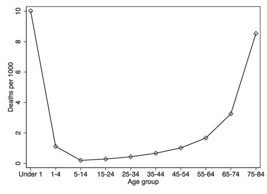
Pneumonia incidence by age, United States, 1935. This figure shows the average pneumonia mortality rate by age group in 1935 in the United States. Figure is drawn by authors using data sourced from Britten (1942).
In addition to reducing mortality, the arrival of sulfa drugs led to significant reductions in morbidity (Hodes et al. 1939; Moody and Knouf 1940; Greengard et al. 1943). Prior to the introduction of antibiotics, pneumonia was a debilitating disease with typical spells often lasting 39 days on average, and children tending to have recurrent spells (Britten 1942). Sulfa drugs reduced the severity and length of these episodes (Connolly et al. 2012), and this was documented in clinical trials among hospital inpatients (Moody and Knouf 1940; Greengard et al. 1943). A reduction in pneumonia morbidity among children thus considerably increased the disposable time of women, who were the main care-givers for children and the sick. By strengthening the infant health endowment, it will have also led parents to move along the quantity–quality indifference curve, trading up quantity in favor of quality. Consistent with this (and despite negative selection into survival following the positive shock of antibiotic access), children born after 1937 who survived to adulthood had significantly better indicators of educational attainment, employment, income, and lower disability (Bhalotra, Clarke, and Venkataramani 2022a). This is a marker of the substantive importance of pneumonia mortality decline among children born in the sulfa era and a result that is consistent with our finding of a decline in intensive margin fertility.7
2.2. Fertility and Fertility Control in Early 20th Century America
Between 1910 and the mid 1920s, the average number of children per woman stood between 3 and 3.5. Fertility thereafter fell during the Great Depression (to 2.5 children per woman) but rose during WW2 and the post-War (Baby Boom) period (1945–late 1950s). Over this period, there is evidence that women born in the early 20th century were able and willing to practise fertility control (Morgan 1991).8 Before the arrival of the birth control pill in the 1960s, couples used diaphragms, latex condoms, vaginal suppositories, withdrawal and douching techniques (Engelman 2011), with the invention of the diaphragm in 1882 being particularly crucial to the advent of effective fertility control by women.9
2.3. Trends in Women’s Labor Force Participation and Marriage
In the 1930s, there was a substantial increase in female labor force participation; for example, there was an increase of 15.5 percentage points, from 10% to 25%, on the extensive margin among married women (Goldin 2006). Marriage and fertility choices were closely related in this period, with only 8.5% of births being out of wedlock (Bachu 1999).10 Previous work has argued that important drivers of the increase in labor force participation in this period included higher rates of high school completion, the arrival of “nice” jobs, such as secretarial work in offices that reduced the stigma associated with married women working, and the virtual elimination of marriage bars by the early 1940s.11 Regardless of education, most working women were engaged in typing-oriented jobs and teaching (Goldin 2006).
3. Birth Timing
This Section presents the data, empirical specification, results and an extensive series of robustness checks for analysis of impacts of antibiotic exposure on birth timing among women who were of reproductive age when the antibiotics first became available. As indicated earlier, we find that the antibiotic-led decline in pneumonia mortality resulted in a decline in fertility on both the intensive and the extensive margins. As the extensive margin result is contrary to the predictions of Aaronson, Lange, and Mazumder (2014), we develop an extension of their model in Section 4, which is consistent with our result. Our model generates predictions for the impact of mortality decline on childlessness, the labor market and marriage outcomes, which we investigate in Section 5.
3.1. Data
Data on individual outcomes are taken from the United States Census Microdata (Ruggles et al. 2010). Online Appendix A describes the data in more detail, including sources and variable definitions. Below, we discuss the birth and mortality data.
Birth Timing Data.
To model fertility during the sulfa era, we use pooled census microdata using the 1940 and 1950 1% samples.12 We select women who were of childbearing age (15–40) at any time between 1930 and 1943 and expand the data to create a woman-level panel, with observations for every year in which a woman was at risk of giving birth. We only include woman–year observations in which a woman was aged 15–40 in that year, so that we capture choices during the fertile period. Thus, the cohorts in the “birth hazard sample” were born in the years 1890–1928.
We use a measure of net fertility that derives from a record of the children living in the mother’s household at the time of enumeration.13 Using a variable that links child records to mothers, we constructed a complete history of live births for each woman, restricting births to biological births (95% of children in the household) that occurred in the United States. As is standard, this measure excludes any pregnancies that did not result in live births, and any deaths that occurred after birth but before the census. It also excludes any children that had left home. The latest census we use is the 1950 census, where the oldest child born during the estimation period 1930–1943 would have been 20, which minimizes concerns about missing older children. In Section 3.4, we discuss estimates that measure fertility using only information on children under the age of 10 at the time of the census.
Mortality Rate Data.
We gathered data on diseases treatable with sulfa drugs and also for diseases that were not treatable, and that thus act as placebos. These data are from several volumes of the U.S. Vital Statistics (Bureau 1930–1943; Linder and Grove 1947; Grove and Hetzel 1968; Ruggles et al. 2010). We create the pre-intervention or baseline levels of cause-specific mortality rates as the state-level average over the years 1930–1936 of the mortality rate, which allows us to smooth over fluctuations in the rate created by influenza epidemics. There are no annual time series data in this era for pneumonia mortality. Instead, the Vital Statistics data contain the mortality rate from pneumonia and influenza combined. This is because the two diseases shared symptoms such as cough and fever, making them difficult to distinguish. Moreover, they were intrinsically related since pneumonia often followed as the more serious development of an initial influenza infection. Importantly for our purposes, because influenza is viral, it was not treatable with sulfa drugs but pneumonia, which includes a bacterial strain, was. Thus, a sulfa-driven decline in the combined influenza–pneumonia mortality rate reflects a decline in pneumonia mortality. Henceforth, for ease of exposition, we refer to this combined rate as pneumonia mortality.
We found decadal data that provide separate series for pneumonia and influenza to strengthen faith in this approach. First, these data show that pneumonia dominated the combined mortality rate, being responsible for 8.9 deaths per 1,000 in 1930, compared with 1.3 deaths per 1,000 live births from influenza. Second, the decline in the combined mortality rate between 1930 and 1940 was entirely on account of a decline in the pneumonia mortality rate: Influenza rates fluctuated considerably with epidemics and seasons, but the average influenza rate was steady across the decade.
In a similar vein, we use the all-age pneumonia and influenza mortality rate on the grounds that both the level and the trend are driven by the infant rate. Infant births and deaths, the two components required to calculate infant and child mortality rates, were known to be under-reported in this era (Eriksson et al. 2018; Linder and Grove 1947), making the child rate noisier than the all-age rate. In addition, under-reporting may have been more prominent in the Southeastern United States, where rates of pneumonia were higher on average, and this could result in systematic measurement error (Ewbank 1987). We show below that infant and child pneumonia mortality was the overwhelming source of variation in the all-age rate, and provide additional detail on the extent of mismeasurement in child mortality rates. In order to create a measure of women’s health distinct from adult health, we obtained gender- and cause-specific mortality rates, and age- and cause-specific mortality rates for the study period from Vital Statistics, which we incorporate in a specification check discussed in Section 3.4.
Summary Statistics.
Tables A.1 and A.2 in the Online Appendix provide descriptive statistics. The woman–year observations are balanced before and after the intervention, with an annual mean probability of birth of 8.7%. All-age pneumonia and influenza mortality before the intervention was on average 1.09 per 1,000 population.
3.2. Empirical Strategy
We begin by documenting the “first stage” impacts of the introduction of sulfa antibiotics on pneumonia mortality, demonstrating a nationwide trend break in 1937, and that this was larger in states with higher baseline rates of pneumonia mortality. As a result, the introduction of sulfa drugs drove convergence in pneumonia mortality across states. We then describe an empirical strategy that identifies the impact of sulfa drugs on fertility timing.
Trend Break in Pneumonia Mortality.
The timing of the introduction of antibiotics created sharp variation across cohorts in exposure to pneumonia, a disease treatable with sulfa drugs. Figure 2 shows trend breaks in pneumonia mortality in 1937. Pneumonia mortality declined on average 8.1% per year from 1937: See panel A in Online Appendix Table B.1 that shows the coefficients in regressions of pneumonia mortality that allow for a linear trend break in 1937. Most deaths from pneumonia occur in infancy, when the immune system is still fragile, and the steepest post-sulfa decline in pneumonia mortality was amongst infants and young children (see columns (2) and (3) of Online Appendix Table B.1).14
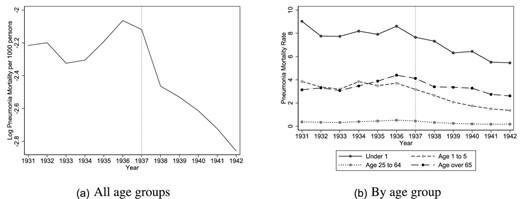
Pneumonia mortality, United States. These figures show the log average pneumonia mortality rate for all ages (left) and by age group (right) in the United States over time. Source: Vital Statistics.
State Convergence in Pneumonia Mortality.
There was considerable geographic dispersion in pre-intervention levels of pneumonia mortality (Figure C.6 in Online Appendix C.1). Because sulfa drugs led to larger declines in pneumonia in states where the pre-intervention burden was higher, we see post-sulfa convergence in pneumonia mortality rates across the U.S. states (Figure 3). In column (4) of Table B.1, the estimated convergence coefficient for pneumonia mortality is -0.29, implying that a sulfa-led decline in pneumonia mortality equivalent to an interquartile shift in the pre-intervention pneumonia mortality distribution (-0.26) was associated with a 7.5% reduction in pneumonia mortality.
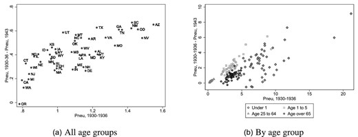
Pneumonia mortality convergence post-1937, United States. These figures show the relationship between the 1937–1943 absolute change and the 1930–1936 average level of pneumonia mortality for all age groups (left) and by age group (right) across the states of the United States. Source: Vital Statistics.
Estimating Equation for Birth Timing.
Identification exploits these two features of the antibiotic revolution—the post-1937 decline in mortality rates and the large variation across U.S. states in pre-intervention levels of the disease burden, in a difference-in-differences design similar to that in Acemoglu and Johnson (2007), Bleakley (2007), Ager, Hansen, and Jensen (2017), and Bhalotra and Venkataramani (2011). The event of the nationwide introduction of sulfa drugs in 1937 was plausibly exogenous, being the direct result of scientific innovation. However, the identifying assumption of parallel counterfactual trends in fertility in states with higher versus lower pre-1937 levels of pneumonia merits scrutiny. We elaborate our approach to this below.
We analyze births in a short window around 1937, namely 1930–1943. This limits the role of confounding events, such as the influenza epidemic of 1928 and 1929 and the increasingly widespread use of penicillin after 1943. We restrict the sample to women of reproductive age (and hence at risk of birth) during this period. Using longitudinal birth history data for these women, we estimate impacts of the discrete event of antibiotic availability on birth timing. (The probability that a given woman gives birth in a given year.) The estimation equation is
where |$Y_{jsctr}$| is a binary indicator that equals 1 if woman j born in state s, census region r, and cohort c, gave birth in year t, and 0 otherwise. The variable |${post-1937}_{t}$| equals 1 if the potential birth year of the child is 1937 or after, and 0 otherwise, as 1937 marks the nationwide introduction of antibiotics. |${prePneumonia}_{s}$| is the 1930–1936 (baseline) average state level pneumonia mortality rate. The coefficient of interest is |$\alpha _{1}$|, which captures the causal effect of the antibiotic-led pneumonia mortality decline on the probability of birth. We estimate equation (1) as a logistic regression, yielding estimates for a discrete time proportional hazard model. Standard errors are clustered at the birth state level to account for serial correlation in outcomes within states (Bertrand, Duflo, and Mullainathan 2004).
The equation includes indicator variables for years since last birth with the count starting at age 15 and restarting after every birth (|${timesincelastbirth}_{jt}$|), and indicator variables for the birth order of the next birth (|${birthorder}_{jt}$|). We include fixed effects for the woman’s race (|${race}_{j}$|), education (|$education_{j}$|), birth state (|$\kappa _{s}$|), and birth year (|$\phi _{c}$|). The other, state-level control variables are discussed below. Education will in part capture potential wages and fertility preferences. In a robustness check, we also allow for woman fixed effects, which will capture any unobservables that determine compliance and are potentially correlated with fertility preferences.
Extensive and Intensive Margins of Fertility.
In order to distinguish between the extensive and intensive margins of fertility timing, we estimate equation (1) on subsets of the sample, where we only include woman–year observations in which the woman is at risk of giving birth to her first child (extensive margin), and then to observations where the woman is at risk of giving birth to her second or higher-order child (intensive margin).
Identifying Assumptions.
The main threat to identification is that the variable |${prePneumonia}_{s}$| captures not just baseline pneumonia but also other state-level variation in pre-sulfa conditions that are correlated with both pneumonia and the outcome (fertility). The likely candidate confounders are the disease epidemiology of the state and economic development. For the first, we leverage the fact that sulfa drugs were able to treat some diseases and not others to identify a set of placebo diseases, which we control for. For the second, we assimilated data on indicators of income, health and education spending, infrastructure and women’s labor market position, and condition on these. Each of these variables is included as its pre-intervention value interacted with an indicator for post-intervention cohorts (|${statecontrols}_{s}\ast {post1937}_{t}$|). This sharpens the test as it allows structural breaks in the controls to coincide with the structural break in pneumonia in 1937. The baseline model includes these controls. In extensions shown as specification checks, we (a) drop all of these controls to assess sensitivity of the estimates to them and, (b) run a far more demanding specification in which each state variable is interacted with a full set of year-fixed effects rather than with the dummy variable |${post1937}_{t}$|.
Tuberculosis and diarrhea were highly prevalent infectious diseases that act as natural placebos. Tuberculosis is a respiratory disease similar to pneumonia in causes but not treatable with sulfa drugs. Diarrhea was also not treatable with sulfa, and it stood alongside pneumonia as a leading cause of death of infants.15 We also control for malaria, another communicable disease as, in this era, there were state-specific interventions including sanitation, housing, and public health programs targeting malaria. We control for mortality rates from cancer and heart disease, the main non-communicable diseases, in order to capture changes in health care quality and access, allowing for state-specific expansion of hospital care. Together, these five placebo diseases control for the state level disease environment.
To distinguish sulfa-driven convergence in pneumonia mortality rates from an underlying process of economic convergence, we control for the logarithms of per capita state income, public health spending, education spending, and the numbers of schools, hospitals and physicians, women’s literacy and women’s labor force participation.16
We address common concerns with controls for observables. First, to allow for the possibility that the underlying confounders are poorly measured (e.g. state income may not fully capture economic development), we follow Pei, Pischke, and Schwandt (2018) and perform a version of a balance test, which involves regressing each of the state-level economic and disease variables on the sulfa exposure variables. Second, we additionally allow for unobservable trends by including census region * year fixed effects (|$\theta _{t}\times {region}_{r}$|) in the baseline model. These control flexibly, for example, for regional differences in impacts of the recession of 1937 and 1938. In alternative specifications, we include finer-grained census division * year fixed effects and state-specific linear trends. As a specification check, we also directly estimate pre-sulfa trends in high versus low pneumonia states and show that they are not statistically significantly different. Third, we estimate impacts of a placebo intervention using an approach similar to that in Aaronson, Lange, and Mazumder (2014). Fourth, to address the possibility of mean reversion, we control for the state-level pre-sulfa average of the outcome variable. Finally, we scrutinize pre-trends and dynamic impacts in event study style models. The event study models show pre-event trends, the dynamic evolution of post-event impacts, and they naturally provide validation of the timing of the event.
Coincident Events.
Even if the identifying assumption of parallel counterfactual trends holds, we need to be sure that we do not capture impacts of other events that happened to coincide with the introduction of sulfa drugs. We already address this in allowing impacts of the 13 state-time varying controls to break in 1937. If there were a policy or other event that occurred in 1937—for instance, a sharp change in income or in a placebo disease—and if this change impacted fertility, our estimates are conditional upon this. (Though to explain our findings this change would need to vary systematically with the pre-1937 level of pneumonia mortality.)
Our baseline model also controls for a trend break in maternal mortality in 1937 that was the result of sulfa drugs being able to treat puerperal sepsis (variable |${preMMR}_s$| in equation (1) above). This is an ascending bacterial infection of the reproductive tract that can occur soon after birth (Thomasson and Treber 2008) and that accounted for 40% of the 6.4 maternal deaths per 1,000 live births in 1930 (Vital Statistics). The maternal mortality rate declined by around 10% per year after 1937 and, in principle, this may have directly influenced the outcomes we study.17
In additional specification checks, we account for impacts of the main historical events of the time, including WW2, the Great Depression and New Deal spending, and the Dust Bowl, demonstrating that our results continue to hold.
Migration and Related Concerns.
In assigning pre-intervention mortality rates and state-level controls to women, we use their birth state because migration decisions after birth are potentially endogenous. We also omit migrants in the main specification. As a result, we may under-estimate treatment effects for women who moved into areas with the largest health gains. To investigate this further, we re-estimate the equation assigning all state-level variables to the resident state of the woman at the time of census enumeration, and also instrumenting state of residence mortality decline with birth state mortality decline—see the discussion in Section 3.4, where we also discuss modeling migration as an outcome and find no evidence of endogenous migration. Among other robustness checks, we investigate sensitivity to age at census sample, and to removing outlier states. We show that the significance of the estimates is robust to a multiple hypothesis testing correction. In Section 3.4, we also discuss and assess our measure of fertility, checking for any bias induced by counting only children at home.
Woman Fixed Effects and Other Specification Checks.
As we created longitudinal data on births within women, we can assess changes in the probability of birth for a given woman post- versus pre-sulfa, conditional on her age. We do this by including woman fixed effects in the model in a robustness check. This takes care of any concerns over unobservables that (endogenously) determine selective uptake of sulfa drugs for pneumonia and are correlated with fertility preferences. While the baseline model is estimated as a logistic regression, we show that estimating equation (1) as an Ordinary Least Squares (OLS) regression produces broadly similar estimates.
Measurement Error in Mortality Rates.
We use the all-age pneumonia mortality rate rather than the infant or child rate to capture exposure because child mortality was measured with greater error (Ewbank 1987; Eriksson et al. 2018; Linder and Grove 1947). The reason the all-age pneumonia rate is a good proxy for the child rate is that the all-age rate is dominated by the child rate, with the child pneumonia mortality rate being 29 times as large as the adult rate. To defend our choice, we supplement the existing historical evidence with new evidence of greater measurement error in child than in adult pneumonia mortality. Essentially, we leverage the variation across the states in the years in which they joined the national system for registration of births and deaths. Joining the national system led to adoption of best practices, resulting in improvements in data quality, which were increasing in time since joining. We compare states joining early versus late, and test for greater dispersion in child versus adult mortality rates in the late versus the early joiners (see the discussion in Section 3.4). We cannot and do not rule out that the reduced form estimates of impacts of the antibiotic innovation capture impacts on women’s health alongside their impacts on child health and mortality. However, as the prevalence of pneumonia among adults was many times lower than among children, and as the identified changes in the outcomes are fairly large, we argue that the identified impacts are unlikely to be driven by improvements in women’s health alone. To back this, we investigate adding controls for female- and cause-specific mortality rates to the baseline regression to test whether this attenuates the coefficient of interest. Our theoretical model carefully traces the mechanisms by which the studied outcomes respond to a decline in child mortality, but in an extension, we also discuss how they respond to an improvement in women’s health.18
3.3. Birth Timing Results
We find that the conditional probability of birth declined following sulfa-led reductions in pneumonia mortality (panel A, Table 1). Notably, fertility declined on the intensive and extensive margins (see columns (2) and (3)).19 We scale our estimates using an interquartile shift in (baseline) pneumonia mortality (-0.26), which is close to the actual nationwide decline that took place after 1937.
Probability of birth as a function of sulfa exposure.
| (1) | (2) | (3) | ||
|---|---|---|---|---|
| A: Main estimates | Birth | Extensive margin | Intensive margin | |
| |${ {prePneumonia}}\ast {post1937}$| | |$-0.0233^{**}$| | |$-0.0121^{**}$| | |$-0.0113^{**}$| | |
| (0.0100) | (0.0060) | (0.0051) | ||
| N | 4,499,588 | 2,894,976 | 1,604,612 | |
| Mean | 0.0865 | 0.0513 | 0.1491 | |
| (1) | (2) | (3) | (4) | |
| B: Specification checks | Birth | |||
| w/out state | w/yr interact | State trend | Division*year | |
| controls | FE | |||
| Birth | ||||
| |${ {prePneumonia}}\ast {post1937}$| | |$-0.0143^{***}$| | |$-0.0100^{***}$| | |$-0.0218^{*}$| | -0.0288|$^{***}$| |
| (0.0033) | (0.0034) | (0.0127) | (0.0092) | |
| N | 4,558,873 | 4,499,588 | 4,499,588 | 4,499,588 |
Notes: The dependent variable is a dummy variable that equals 1 if the woman gave birth in that year, and 0 otherwise. |${prePneumonia}\ast {post1937}$| is the average state-level pneumonia mortality rate between 1930 and 1936, interacted with a dummy variable for the years 1937 and later. These are marginal effects from logistic regressions with standard errors (in parentheses) clustered at the woman’s birth state level and the table shows marginal effects at the means of all covariates in the estimating sample. In panel B, column (1) removes state-year varying controls, column (2) adds allows the state-year controls to have flexible coefficients by year, column (3) replaces the census region-year fixed effects with state linear trends, and column (4) replaces them with census division*year fixed effects. *denotes p-value < 0.1, **denotes p-value < 0.05, and ***denotes p-value < 0.01.
This implies a 0.6 percentage point reduction in the annual probability of birth, which relative to the annual mean of 8.6% before 1937 is a reduction of 6.9% (column (1)). The estimates in column (2) for the extensive margin response imply a 0.3 percentage point reduction in the annual probability of transitioning to motherhood after 1937, which is 5.9% of the pre-intervention mean of 5.1%. For a woman exposed to sulfa drugs for 10 years of her fertile period, this is a 3 percentage point increase in the probability of being childless.
The intensive margin result shows that the same interquartile shift implies a 0.25 percentage point reduction in the probability of transitioning to a higher order birth after 1937, which is 1.7% of the pre-intervention mean of 14.9%.20 Thus, the decline in pneumonia mortality delayed the transition to first and higher order births. The delay to the first birth was about three times the delay to higher order births, which is consistent with the impact of sulfa exposure on childlessness that we document in Section 5 below.
Event Study for Birth Timing.
We estimate an event study specification for probability of birth similar to column (1) of Table 1, where we interact baseline pneumonia mortality with indicators for every year in the sample period (1930–1943, with 1937 as the base year). Marginal effects calculated from the log odds coefficients in the logit regression are plotted in Figure 4. While this exercise is challenged by statistical power and not all coefficients are statistically significant, the plot suggests a discrete change in 1937, with a decline in birth probability for women who experienced larger declines in pneumonia mortality. This plot also provides a test of the identifying assumption that pre-trends in birth outcomes in states with high versus low pre-intervention disease burdens were not different, insofar as the coefficients show no trend before 1937. Overall, our findings show that women delayed childbearing in response to improvements in child survival and child health.
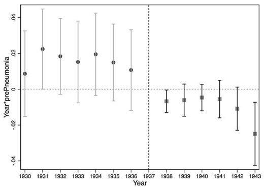
Event study: Probability of giving birth over time as a function of pneumonia mortality decline. This figure displays the marginal effects from logit coefficients and |$95\%$| confidence intervals around these effects on the set of variables |${ prePneumonia}\ast { year}$|, where |${ year}$| is a set of dummy variables for the 13 years 1930–1936 and 1938–1943 (1937 is the omitted case). The dependent variable is a dummy variable that equals 1 if the woman gave birth in that year, and 0 otherwise.
3.4. Robustness Checks
We now discuss results of robustness checks motivated in the empirical strategy section.
Omitted Trends.
While we have a clean policy experiment in the introduction of the drug, we need to be sure that baseline levels of pneumonia mortality are not capturing other baseline conditions. The event study mitigates this concern. We nevertheless use pre-sulfa data to directly model trends. We regress the probability of birth in the pre-sulfa era, 1930–1936, on a linear time trend interacted with a dummy variable equal to 1 for states with above median mortality, and 0 otherwise. The results, in Online Appendix Table C.20, show no evidence of differential pre-trends across high and low mortality states in the hazard sample.
The most likely candidate confounders in our setting are economic development and the disease epidemiology of the state. Our baseline specification controls for trends in 15 indicators of state-level disease prevalence, income, infrastructure, women’s labor force participation, and an indicator for changes in the quality of birth and death surveillance. Here, we first assess sensitivity of the coefficient of interest to dropping these controls. The coefficient remains statistically significant but is smaller in absolute terms (column (1), panel B, Table 1). We then enrich the baseline specification by interacting all state-level control variables with a full set of year dummies (instead of with just the indicator for post-1937). Although this adds 165 control variables to the specification, and renders the coefficient of interest smaller, it remains statistically significant and negative (column (2), Table 1). We next enrich the model by controlling for state occupational structure in 1930 interacted with |${post1937}$| (column (6), Table 2).21 The estimates are robust to this check.
Probability of birth as a function of sulfa exposure—robustness checks.
| (1) | (2) | (3) | (4) | |
|---|---|---|---|---|
| WW2 | New Deal | Dust Bowl | Excl 1939+ | |
| Birth | ||||
| |${prePneumonia}\ast {post1937}$| | |$-0.0239^{**}$| | |$-0.0247^{**}$| | |$-0.0247^{**}$| | |$-0.0256^{**}$| |
| (0.0105) | (0.0107) | (0.0106) | (0.0113) | |
| N | 4,053,834 | 4,499,588 | 4,053,176 | 3,417,407 |
| (5) | (6) | (7) | (8) | |
| Mean reversion | Occ structure | Adult mort | Women’s mort | |
| rates | rates | |||
| Birth | ||||
| |${prePneumonia}\ast {post1937}$| | |$-0.0251^{**}$| | |$-0.0235^{***}$| | |$-0.0332^{***}$| | |$-0.0163^{*}$| |
| (0.0103) | (0.0068) | (0.0122) | (0.0086) | |
| N | 4,499,588 | 4,499,588 | 4,499,588 | 4,499,588 |
Notes: See notes to Table 1 for a description of the baseline regression. Column (1) restricts the sample to births occurring before 1942, Column (2) adds New Deal spending interacted with |${post}$|, Column (3) removes the Dust Bowl states (New Mexico, Oklahoma, Texas, Nebraska, Kansas, and Colorado), Column (4) excludes all births from 1939 onwards, Column (5) controls for the state mean value of |${birth}$| before 1937 interacted with |${post}$|, Column (6) adds the share of women in primary, secondary, and tertiary occupations in 1930 interacted with |${post}$|, Column (7) removes heart disease, cancer and TB all-sex mortality, replacing it with all-sex mortality from these diseases in the age group 20–64, and also adds adult diarrhea mortality (malaria mortality is only available as an all-age rate so remains present as in the baseline specification), and Column (8) removes malaria, heart disease, cancer, and TB all-sex all-age mortality, replacing it with women’s all-age mortality from these diseases, as well as women’s over-2s diarrhea mortality. (The baseline already includes diarrhea mortality among under-2s.) *denotes p-value < 0.1, **denotes p-value < 0.05, and ***denotes p-value < 0.01.
We allow for the possibility that the underlying confounders are poorly measured (e.g. state income may not fully capture economic development), following Pei, Pischke, and Schwandt (2018) and perform a version of a balance test. We regress all of the state-level variables on the sulfa exposure variable.22 Of the numerous tests, only one is statistically significant, which is the coefficient on pneumonia exposure in the equation for TB mortality. Investigating this by estimating an event study model for TB mortality decline, we see a secular decline with no break in 1937.
We residualize pneumonia mortality by all our state control variables, and show the spatial dispersion of residualized pneumonia mortality across the United States in Figure 5. This illustrates that residualized pneumonia mortality is well dispersed. To provide evidence that our results do not capture differences in trends between regions of the United States, we show estimates of the hazard model, where we omit the mountain west and deep south states in turn (Online Appendix Table C.12, columns (3) and (4)).23 This does not substantially change the estimates.
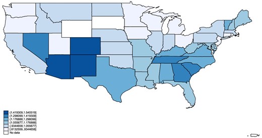
Values of residualized pneumonia mortality across the United States. This figure shows values of pneumonia mortality across the United States that have been residualized in a state-level regression by all the control variables included in the main regressions.
Recognizing that however rich the set of observables is, there are potential unobservables, the baseline specification in the hazard model includes census region-year fixed effects. The estimates are similar in magnitude and not statistically different when we instead include state linear trends or the more fine-grained census division-year fixed effects (columns (4) and (5), panel B, Table 1). We assess mean reversion by controlling for the state-level pre-sulfa (pre-1937) average value of the outcome variable interacted with |$post$| and find it does not change the coefficient of interest (see column (5) in Table 2).
Coincident Events.
Inference with our research strategy relies on getting the timing of the introduction of antibiotics right. For this, we rely on documentary evidence that the advent of sulfa drugs was widely publicized, for example, in a New York Times article in December 1936 (“Conquering Streptococci”), and that historians have documented widespread uptake in 1937 (Lesch 2007). Online Appendix Figure C.7 shows extracts from two articles that appeared in the New York Times in 1936. The first stage trend break plot for pneumonia and the event study for fertility both confirm that the structural break in trend was in 1937.
Still, we may be concerned that these changes were driven by a coincident event rather than by the arrival of sulfa drugs. The United States entered WW2 in December 1941. To assess the relevance of this, we restrict the sample to births occurring before 1942. Our findings are essentially unchanged (column (1), Table 2). To capture potential impacts of the Great Depression and subsequent recovery, we accessed data on state-year data on New Deal spending (Fishback, Kantor, and Wallis 2003) and included this as a control, interacted with sulfa exposure (|${post1937}$| in the hazard model). The coefficients of interest are robust to this (column (2) in Table 2). The Dust Bowl refers to a period of drought and dust storms during the 1930s that damaged agriculture in several southern U.S. states and resulted in large out-migration from those states.24 The results are, if anything, strengthened by the omission of the Dust Bowl states (column (3), Table 2).
Sulfa drugs were available without prescription until 1939. Our findings are similar when we exclude all births after prescription was introduced (column (4), Table 2). We also verify that the coefficients on pneumonia mortality decline are not significantly different when omitting maternal mortality decline (columns (2) and (3) in Online Appendix Table C.25). Finally, the 1930s and 1940s did experience some increases in childcare provision, particularly during WW2, in order to encourage female employment. However, the Lanham Act was not implemented until 1943, and provided only 130,000 spaces for children (far short of the intended 2 million), and these child care centres were quickly closed down after WW2.
Measurement Issues with Fertility.
We consider potential concerns with the way that we measure fertility. First, we measure fertility using information on children living at home in census data. As a check on this, we only include potential births from the 1950 census that would have occurred in the years 1940–1943: This way, the oldest child would have been 10 (Online Appendix Table C.12, column (1); the results are similar). Second, the conception date is a more accurate measure of a woman’s fertility choice than the birth date of the child. We proxy a child’s date of conception as 1 year before the date of birth, and re-estimate the hazard model using the date of conception as the outcome rather than the date of birth (Table C.12, column (2)) and again the estimates are similar.25
Endogenous Migration.
If prospective mothers migrated in response to disease, then the introduction of sulfa drugs may have influenced migration patterns. In the baseline sample, we omit migrants, defined as women whose birth state is not the same as their state of residence at enumeration. If we instead include these women, and instrument for mortality decline exposure in their state of residence using mortality decline exposure in their birth state, the results are unchanged (Online Appendix Table C.19, columns (1) and (2)). We modeled migration as a function of post-sulfa declines in pneumonia and maternal mortality using two different indicators for migration. First, we defined an indicator for migrants as individuals for whom the birth state is different from the census enumeration state. Second, we defined an indicator for migration between 1935 and 1940 using the information from the 1940 census. The estimates in Online Appendix Table C.19 show no evidence that sulfa-induced changes in mortality rates influenced migration.
All-Age Versus Child Pneumonia Mortality.
Birth and death surveillance in the sulfa era was not as comprehensive as it is today and the quality of vital statistics data varied across the states of the United States. We seek to illuminate measurement error in child mortality rates by leveraging the fact that measurement error declined when a state joined the National Registration System. Joining the national system involved agreeing to adopt a set of best practice guidelines with regard to vital statistics recording. All states had transitioned before the introduction of sulfa drugs, but we exploit relevant variation in the duration for which they had been in the system (Shapiro and Schachter 1952), displayed in Online Appendix Figure C.2.26 In general, we cannot directly ascertain measurement error because we do not have true values of mortality rates. However, historical audit studies have identified inaccuracies in birth registration by comparing state-level vital statistics with census birth counts. Importantly, this gap is larger among late entrants into the National Registration System, a result that validates our use of date of entry to the national system for analysis of measurement error in death counts (Shapiro and Schachter 1952).
On the premise that measurement error is reflected in dispersion, we examine dispersion of child versus adult mortality rates in early versus late entry states, defining early versus late as before versus after 1920, the median year of entry. Using data for 1933–1936, the pre-antibiotic years, we computed the standard deviations of the child (under-5) and adult (ages 25–64) pneumonia mortality rates, scaled by their means (see Online Appendeix Figure C.3). The dispersion in child and adult rates is similar in early entrant states, but in late entrant states the dispersion in child pneumonia mortality rates is substantially higher, consistent with (greater) measurement error in child mortality rates in states with less mature vital registration systems. Online Appendix Table B.2 confirms that year of first participation strongly predicts dispersion in child mortality, but not in adult mortality. Moreover, the share of deaths with missing cause, a proxy for error in cause assignment, fell more sharply and remained consistently lower in early than in late registration states (see Online Appendix Figure C.4).27 Errors in cause of death assignment arise because the symptomology of many diseases, including bacterial pneumonia, more often overlaps with other diseases.28
If we replace the all-age rate in the main analysis with the under-5 pneumonia mortality rate, the result for birth timing is attenuated, but the results for longer run lifecycle outcomes discussed in Section 5 hold (see Online Appendix Table B.3). In the main analysis, which uses the all-age rate, it is possible that an improvement in women’s health ensuing from the advent of antibiotics contributed to the identified changes. To investigate this further, we control for cause-specific female mortality rates or cause- and age-specific adult mortality rates. Recall that we always control for maternal mortality decline. In this specification check, we first add control variables that better reflect women’s mortality risk in terms of age. We include variables measuring adult mortality rates for the placebo diseases.29 Column (7) of Table 2 shows that the birth timing coefficient of interest is stable to this check. Second, we add variables that better reflect women’s mortality risk in terms of gender, adding mortality rates among women rather than all adults. We face data constraints because cause-specific mortality data for women is only available for all ages, but for diseases like cancer and heart diseases that are relatively uncommon among children, the female all-age rate is likely to be a good measure of changes in women’s health. Column (8) in the same table shows the stability of the coefficient on birth probability to these alternative measures of mortality intended to better capture women’s health.30 We investigate the role of women’s health further in Section 5.6, where we make the argument that pneumonia mortality among women (adults) was not prevalent enough to produce the large changes we see in the outcomes of interest, but child mortality was.
Other Checks.
Online Appendix C discusses a number of other specification checks. It shows that our estimates are robust to using alternative age-at-census sample definitions, to adjustment of standard errors for multiple hypothesis testing, exclusion of outlier states and to including woman fixed effects.
4. Theoretical Model: Child Mortality, Fertility, and Labor Market Participation
The preceding section shows that women delayed fertility in response to child mortality decline. The intensive margin result is consistent with the predictions of the classical quantity–quality model, and recent innovations which predict that as health improves and mortality declines, women have fewer children and invest more in each (Becker and Lewis 1973). Aaronson, Lange, and Mazumder (2014) argue that factors like child mortality decline should increase extensive margin fertility by increasing the value of having at least one child. We, however, find a decrease in extensive margin fertility. We hypothesise that this seeming contradiction can be resolved by taking a wider lens, and considering that child health improvements may affect fertility timing and women’s labor market participation. Essentially, when child mortality declines, women can afford to start fertility later to achieve a given fertility target, in addition to which they may lower their target fertility. Fertility delay enables labor market participation and can eventually result in childlessness.31
In this section, we present a new model incorporating dynamic fertility and labor supply choices. We present here the central economic insights from a simple model, and we discuss extensions to this framework in Online Appendix D such as allowing for improvements to women’s health, where we also provide the formal proofs. The model yields predictions not only for extensive margin fertility but also for later life outcomes, including childlessness and labor market participation, which we investigate in Section 5.
4.1. Model Environment
There is a population of women indexed by |$i\in [0,1]$| whose life cycle consists of three periods |$t\in \left\lbrace 1,2,3\right\rbrace $|. Women have utility |$U=A\cdot u\left(n,e\right)+c$|, where |$n\in \mathbb {Z}$| is the (integer) number of their surviving children at the end of the life cycle, |$e\in \mathbb {R}_{+}$| is her choice of child quality, and |$c\in \mathbb {R}_{+}$| is her consumption. We assume that |$u\left(n,e\right)$| is strictly concave and twice differentiable, with |$u\left(0,e\right)=0$| for all e.
We allow for heterogeneity in the preference parameter A, which measures women’s preference for children relative to other consumption. We assume that A has cumulative distribution |$F\left(A\right)$| across women, with density |$f\left(A\right)=F^{\prime }\left(A\right)>0$| for all |$A\ge 0$|.
The timing of events is as follows: At both dates |$t=1$| and |$t=2$|, a woman decides whether to get pregnant. If she gets pregnant, denoted |$a_{t}=1$|, she gives birth to a child, who survives with probability |$1-\lambda$|, where |$\lambda$| is the rate of child mortality. If she does not get pregnant, denoted |$a_{t}=0$|, she can work for a wage |$y_{t}$|. Her potential wage follows a simple stochastic process that captures the “job then family” pattern of the sulfa drug era (Goldin 2004) and is initialized at |$y_{1}=0$|. If she does not get pregnant at |$t=1$|, she is promoted with probability p, in which case her potential wage rises to |$y_{2}=Y>0$|. Otherwise, her wage remains at |$y_{2}=0$|. We also analyze the robustness of our results in the presence of richer income processes, which we discuss below.
At date 3, the woman’s fertility is complete, and she takes as given the final number of her surviving children |$n\in \left\lbrace 0,1,2\right\rbrace $|. She chooses her consumption c and child quality e so as to maximize utility subject to her budget constraint:
The left-hand side of the budget constraint (2) measures her spending on consumption and children. As in the classical quantity–quality model (Becker and Lewis 1973; Aaronson, Lange, and Mazumder 2014), her expenditure on children is |$n(\tau _{q}+\tau _{e}e)$|, where |$\tau _{q}$| is the price of child quantity, and |$\tau _{e}$| is the price of quality per child. Her total wealth, on the right-hand side of the budget constraint, is given by the sum of wages in all periods in which she worked, and an exogenous endowment |$\omega$|. In contrast to Becker and Lewis (1973) and Aaronson, Lange, and Mazumder (2014), where income is exogenous, we endogenize it.
Substituting the budget constraint (2) into the woman’s objective, we find that the woman’s choice of child quality e at date 3 must solve the simplified maximization problem
The function |$V_{n}(A)$| denotes the woman’s surplus, that is, the utility that the woman enjoys at date |$t=3$| over and above consuming her wealth. Note that, for |$n=0$|, surplus is |$V_{0}\left(A\right)=0$| for all A, while the optimal e is indeterminate. For |$n>0$|, suplus maximization is a well-behaved, concave problem in e, and the surplus is increasing in the preference parameter A. With the dynamic decision process we have specified, our model therefore circumvents the potential non-convexity of the classical quantity–quality model, in which n and e are chosen simultaneously.
In this section, we present a simple case that isolates the effects of child mortality on fertility on the extensive margin. We assume that a woman’s surplus is maximized when having at most one child, that is,
For example, if the women’s preferences have the Cobb–Douglas form |$u\left(n,e\right)=e^{\alpha }n^{1-\alpha }$|, then (4) holds if and only if |$\alpha >{1}/{2}$|. In the Online Appendix, we extend our results in an environment without this assumption.
4.2. Optimal Fertility and Labor Supply Choices
We begin by characterizing a woman’s optimal fertility and labor supply choices as a function of the preference parameter A, which measures the strength of her preference for having children. We show that the optimal fertility choice is fully characterized by three scenarios, which we refer to as no fertility, delayed fertility, and early fertility.
There exist two thresholds |$\underline{A}$| and |$\bar{A}(\lambda )$| such that the woman’s optimal policy is as follows:
No Fertility: If |$A<\underline{A}$|, then the woman works at |$t=1$| and at |$t=2$| with probability 1.
Delayed Fertility: If |$\underline{A}\le A<\bar{A}\left(\lambda \right)$|, then the woman works at |$t=1$| and gets pregnant at |$t=2$| if and only if she is not promoted.
Early Fertility: If |$\bar{A}\left(\lambda \right)\le A$|, then the woman gets pregnant at |$t=1$|, and gets pregnant again at |$t=2$| if and only if she does not have a surviving child yet.
and we have |$\bar{A}(\lambda ) > \underline{A}$| for all |$\lambda \in [0,1]$|.
If the woman’s preference A for children is so weak that the surplus |$V_{1}\left(A\right)$| from having a child is negative, then it is never optimal to get pregnant. The second and third points explain the optimal timing of fertility. The proposition establishes that it is optimal for the woman to delay her fertility until |$t=2$| whenever her preference A is strong enough to satisfy the following inequality:
This expression has an intuitive interpretation. The right-hand side of (5) is the marginal benefit of delay in terms of income. By delaying, the woman has a probability p of being promoted, which leads to additional earnings Y. The left-hand side is the marginal cost of delay. To interpret this term, consider the following two effects. On the one hand, a woman who delays will (optimally) remain childless if she is promoted. If not promoted, she would have had a child with probability |$1-\lambda$|. Hence, the possibility of promotion reduces the probability of having a child by |$p\left(1-\lambda \right)$|. On the other hand, a woman who delays has one fewer attempt at fertility, which reduces the probability of having a surviving child by |$\lambda \left(1-\lambda \right)$|. Combining these two effects, delaying reduces the probability of having a child by a total of |$\left(p+\lambda \right)\left(1-\lambda \right)$|. Scaling this probability by the surplus |$V_1 (A)$| associated with having a child yields our expression for the marginal cost. The formal proof of Proposition 1 also verifies the conjecture that it is never optimal for a woman to get pregnant after being promoted. Intuitively, this behavior would be optimal only for women with strong preferences for children, for whom early fertility is a dominant strategy to begin with.32
We can gain additional intuition by re-writing equation (5) as
The right-hand side can be interpreted as the option value of delay, which measures the expected utility gain from getting promoted, which arises with probability p. The left-hand side is the insurance value of early pregnancy. The insurance value of early pregnancy measures the expected utility gain from having a second chance: With probability |$\lambda$|, the first pregnancy does not survive, but the second survives with probability |$1-\lambda$|. The second chance thus adds value |$V_{1}(A)$| with probability |$\lambda (1-\lambda )$|. It is optimal to get pregnant early when the insurance value exceeds the option value of delay.
Next, we derive the overall probability of childlessness in the population of women. This probability is a key object of our empirical analysis in the next section, where we study the impact of sulfa drugs on childlessness.
The probability that a woman in the population is childless at date 3 is
This proposition evaluates the probability of childlessness in each of the three cases that govern the optimal choice, weighted by the mass of women that fall into each case. The top line in equation (7) is simply the fraction of women with no fertility. The middle line is the fraction of women with delayed fertility times their probability of childlessness. This probability is the sum of p, since they are childless if promoted, and |$\left(1-p\right)\lambda$|, since they are childless if they are not promoted but suffer an unsuccessful pregnancy. Finally, the bottom line is based on the fraction of women who choose early fertility. Since these women have two attempts at having a child, their probability of childlessness is lower and equal to |$\lambda ^{2}$|.
4.3. The Effect of Shocks to Child Mortality
We now characterize the effects of a change in the rate |$\lambda$| of child mortality on women’s incentives.
The optimal choice, as characterized in Proposition 1, responds to changes in the child mortality rate |$\lambda$| as follows:
The threshold |$\underline{A}$|, at which a woman switches from no fertility to delayed fertility, is independent of |$\lambda$|.
- The threshold |$\bar{A}\left(\lambda \right)$|, at which a woman switches from delayed to early fertility, satisfies |$\frac{\partial \bar{A}}{\partial \lambda }<0$| if and only if |$\lambda$| satisfies(8)$$\begin{eqnarray} \lambda <\frac{1-p}{2}. \end{eqnarray}$$
The first point in this Proposition is that the boundary between no fertility and early fertility does not change in response to a change in |$\lambda$|. This is because no fertility is chosen only by women who perceive negative surplus from having a child. The boundary is therefore at the point where surplus (as defined in (3)) is 0, which is independent of |$\lambda$|.
The second point shows that incentives to delay are decreasing in |$\lambda$|, as long as |$\lambda$| is not too large. This is because an increase in |$\lambda$| raises the marginal cost of childlessness by reducing the likelihood of success for a woman who has only one attempt at having a child.33
Figure 6 provides a numerical illustration of these effects. The figure considers a range of values for |$\lambda$| along the horizontal axis and a range of preference parameters A on the vertical axis. Motivated by the empirical setting, we focus on values for the child mortality rate |$\lambda \le 15\%$|. We plot the regions in which women choose no fertility, delayed fertility, and early fertility. Consistent with Proposition 3, panel (a) shows that the region of delay widens when |$\lambda$| declines, as women switch their behavior away from early fertility. For the same preference parameter, a woman is more likely to delay her fertility as child mortality declines. Panel (b) shows that the pattern also holds, and indeed becomes more pronounced, if the woman is fertile for a greater number of time periods. (See our discussion of the general dynamic model below and in Online Appendix D.3.)
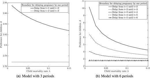
Numerical example: The effect of a reduction in child mortality on fertility delay. The figure plots the critical values of the preference parameter A, which measures the strength of the preference for children, as a function of the rate |$\lambda$| of child mortality. If A is above the top line in panel (a), then it is optimal to get pregnant early at |$t=1$|. If A is between the top and the bottom line, then it is optimal to delay fertility |$t=2$|. If A is below the bottom line, then no fertility (or, equivalently, delay until |$t=3$|) is optimal. The region of delay becomes wider as |$\lambda$| declines. Similarly, panel (b) shows the optimal regions of pregnancy timing for a model with 6 periods. The parameter values are |$\tau _q=\tau _e=2$|, |$u(n,e)=A e^{\alpha } n^{1-\alpha }$|, |$\alpha = 0.9$|, |$Y=1$|, and |$p=0.1$|.
The interesting and hitherto little recognized implication is that a decline in child mortality can lead to increased incentives to delay fertility. Several extensions to our model, which we discuss in detail below, show that this finding is robust to enriching the specification. For example, we show that it goes through in environments that feature a richer income process, general dynamic decisions, increasing risks of infertility with age, as well as optimal marriage and career choices.
Before discussing the detailed empirical implications of this result, we characterize its implications for the rate of childlessness in the population as a whole.
The probability of childlessness, as characterized in Proposition 2, responds to a change in the child mortality rate |$\lambda$| as follows:
This result decomposes the effect of a change in |$\lambda$| on the probability of childlessness into two terms. The first line in equation (9) is the mechanical effect of a change in |$\lambda$|, holding women’s behavior constant. This effect is always positive. Any increase in |$\lambda$| mechanically leads to fewer surviving children and, hence, a higher incidence of childlessness. This force affects women who choose either delayed or early fertility. The second line is the behavioral effect that arises from changes in women’s optimal choices. Women with |$A=\bar{A}(\lambda )$|, who are indifferent between early and delayed fertility, switch their optimal strategy in response to a marginal change in |$\lambda$|.34 This effect has the sign of |${\partial \bar{A}(\lambda)}/{\partial \lambda }$| and scales with the density |$f(\bar{A}(\lambda ))$| of “switchers”.
Concretely, consider the case where |$\lambda$| is small in the sense of Condition (8). Suppose that there is a beneficial health shock that decreases |$\lambda$|. The mechanical effect is a decrease in childlessness. The behavioral effect, however, is that some women switch from early to delayed fertility, which reduces their overall probability of having children. If the density of switchers is large enough, then the behavioral effect dominates and the overall effect on childlessness is positive.
In a model with a more general income process, there is an offsetting effect whereby a decline in |$\lambda$| can encourage women to switch from no fertility into delayed fertility.35 However, when the density of switchers from early to delayed fertility is sufficiently large, this additional effect is dominated by the effects of increased delay.
4.4. Empirical Predictions
In our empirical analysis, we are interested in the causal effects of a beneficial shock, namely, the introduction of sulfa drugs, which led to declines in both child mortality and child morbidity. As a benchmark, recall the predictions of the classical quantity–quality model of fertility (Becker and Lewis 1973). In this model, women only solve a static surplus maximization problem similar to (3). Beneficial health shocks in this framework are typically modeled as declines in the prices |$(\tau _{n},\tau _{q})$| of child quantity and quality. The empirical implication of the quantity–quality model is that beneficial health shocks always decrease the likelihood of childlessness, because they increase the surplus associated with having at least one child (Aaronson, Lange, and Mazumder 2014).
In contrast to the basic quantity–quality model, our model predicts that a beneficial health shock increases the likelihood of childlessness, as long as it enocourages enough women to delay their fertility. As we have discussed above, a necessary condition for this prediction is that the baseline rate |$\lambda$| of child mortality is not too large, that is, that Condition (8) holds. In our empirical setting, a back-of-the-envelope calculation suggests that this condition is plausible. A population average child mortality rate of 47 per |$1,000$| live births in 1939 (Dowell et al. 2000) implies that |$\lambda ={47}/{1,000}$|, so that Condition (8) is satisfied if the probability of promotion is less than 90.6%.36
The effects of health shocks through prices, which are the focus of the quantity–quality literature, can also be incorporated in our dynamic model. If a health shock decreases the rate of child mortality but also decreases prices, then the effects of lower prices and of decreased mortality push women’s optimal fertility timing decisions in opposite directions. In this case, one needs to impose a tighter upper bound than (8) on |$\lambda$| to ensure that a beneficial health shock encourages delayed fertility (see Online Appendix D.2).
In our baseline model, we have focused on extensive margin fertility decisions. In Online Appendix D, we further consider higher birth orders. This leads to an additional prediction, namely, that a beneficial health shock leads to lower numbers of children on the intensive margin, again as long as it leads a sufficient measure of women to delay their fertility.37
The key mechanism in our model is that women have stronger incentives to enter the labor market, and have children later, after a positive health shock. When they do, they benefit from the possibility of being promoted and, if promoted, they remain in the labor market instead of having children. Thus, the model delivers several auxiliary predictions that allow us to test the mechanism behind changes in fertility. Concretely, our model predicts that a beneficial health shock:
leads to later fertility, even among women that eventually have children, also increasing marriage delay and the risk of never marrying (see Online Appendix D.4.4);
increases female labor force participation;
increases the number of women in more prestigious, highly paid employment.
In the next section, we take these predictions to the data.
4.5. Extensions and Robustness
The main novelty in our model is the result, stated in Proposition 3, that declines in child mortality can lead to increased incentives to delay fertility. This is true for parameter values delineated by Condition (8), which is likely to be satisfied in our empirical context. We now discuss a series of extensions to the model. These extensions are analyzed formally in Online Appendix D. In each case, we analyze the equivalents of Proposition 3 and Condition (8) and discuss how they deviate from the baseline model.
1. General dynamics (Online Appendix D.3). We extend the baseline model to T periods. We derive a closed form solution to the Bellman equation associated with optimal fertility timing. We show that, if Condition (8) holds, then a decline in child mortality |$\lambda$| strengthens incentives to delay fertility across the board. For example, the optimal date of the first pregnancy switches from |$t=1$| to |$t=2$| for a range of preference parameters A, from |$t=2$| to |$t=3$| for another range, and so forth. Thus, the qualitative effects in a general dynamic model are the same as in the simple three-period model that we have presented above.
2. Income effects (Online Appendix D.4.1). We consider more general preferences and a richer income process to study the potential implications of income effects. Income effects become relevant when child quality (e.g. education) accounts for a large fraction of households’ expenditure. In this setting, a woman who has worked for one period spends more on child quality and enjoys greater surplus from having a child. Therefore, changes in |$\lambda$| have a stronger effect on the value of delay than on the value of early fertility, which reinforces the mechanism by which health shocks encourage delay. Accordingly, with some natural restrictions on preferences, we show that income effects strengthen our argument in the sense that we now obtain our key results under a weaker condition than (8).
3. Higher birth orders (Online Appendix D.4.2). We relax Assumption (4) so as to incorporate women who wish to have more than one child. Intuitively, the prospect of having several children weakens women’s incentives to delay their fertility. We therefore derive a stronger Condition (8), which guarantee that declines in child mortality encourage fertility delay.
4. Increasing risk of infertility (Online Appendix D.4.3). We consider a model in which the woman risks becoming infertile each period, so that the overall risk of infertility is increasing over time. We show that a slightly stronger condition than Condition (8) is needed to recover our main results in this case. Intuitively, declining fecundity makes delayed fertility less attractive, and also reduces the incentive to switch to delayed fertility after a health shock. Online Appendix Figure D.1 shows that the pattern of increased delay in the numerical example also holds when we allow for increasing risk of infertility.
5. Marriage decisions (Online Appendix D.4.4). For the sample of women in our empirical analysis, the social norm was to leave the labor force and get married before having children. We explore the implications of our model for marriage decisions by assuming that a woman’s first pregnancy is contingent on finding a partner and getting married. We further assume that finding a partner is probabilistic. This feature makes delayed fertility a more risky prospect than early fertility. The economic effects of this force are similar to the case with an increasing risk of infertility, which we have discussed above.
6. Career choices (Online Appendix D.4.5). We analyze the behavior of women who can choose between a risky career with large income upon promotion, such as we have modeled above, and a safe career with a flatter income trajectory. We show that women who plan to delay fertility self-select into risky careers. We also demonstrate that the presence of career choices does not alter the qualitative effects of changes in child mortality.
7. Women’s health (Online Appendix D.4.6). We analyze the impact of a shock to women’s own health and compare it to our baseline analysis, which focuses on shocks to child mortality. We emphasize two effects of women’s health in our model: Healthier women are potentially more productive in the labor market (e.g. Bloom et al. 2020), but also derive greater net utility from having healthy children (e.g. because good health lowers the cost of child rearing). We show that these two effects have opposite implications for fertility choices. In particular, increased labor market productivity strengthens women’s incentives to delay their fertility. By contrast, an increased net utility from childbirth increases women’s incentives to leave the labor market and start their fertility early. As we explain in detail in the Online Appendix, the latter effect dominates women’s responses at the margin when the initial rate of child mortality |$\lambda$| is low.
5. Impacts on Later Life Outcomes: Fertility, Labor Market, and Marriage
In this Section, we bring the data to bear on the theoretical predictions of the model in Section 4. Having already established that sulfa exposure caused women to delay fertility at both the intensive and extensive margins, we test whether it also led to more childlessness, lower completed fertility, higher labor market participation, better careers, and less marriage. We find evidence in support of these predictions.
5.1. Data
As before, we analyze the sample of women who were of reproductive age in a window around the time of the introduction of sulfa drugs. Earlier we studied their birth outcomes during 1930 to 1943. We now track the same cohorts of women into their later life, identifying them in later census years using the 1% microdata samples of the 1940 to 1970 censuses. To model completed fertility, we analyze women who were aged 40–50 at the time of census enumeration.38
We also show results for women of childbearing age (18–40) at census enumeration, to corroborate any impacts on delay that we estimate in the hazard model. The sample includes birth cohorts 1893–1931 who were aged 6–44 in 1937. We exclude women aged 5 and under in 1937 as they were potentially directly treated by antibiotics as children. We include not only women aged 15–40 in the period 1930–1943 (as in the birth timing sample) but also women who would have been exposed to the sulfa drug era throughout their reproductive years (aged 6–15 in 1937) and women who would not have been exposed at all (aged 40–44 in 1937).39 As in the birth timing sample, we focus on net fertility (children resident in the household), but in a robustness check, we also use data on gross fertility (total number of live births) to show that both measures yield comparable estimates. Data on labor market and marriage outcomes are from the same census files, and we model outcomes for women aged 18–50 at the time of the census.
Online Appendix Table A.2 provides a descriptive statistics. Using net fertility (based on surviving children) among women of childbearing age at the time of the census, the average woman was exposed to sulfa drugs for 20 years, and 36% of women were childless, with 1.7 births in total, and 2.6 conditional on at least one. Among women who had completed their fertility at the time of the census, the average woman was exposed to sulfa for 14.6 years, 28% of women were childless at the end of their reproductive years, average total fertility was 1.9 (unconditional on at least one birth) and 2.7 conditional on at least one. The mean age at first birth in the stock sample was 24.1, and 26.7 at second birth. In the labor maket sample, 37% of women were in the labor force, and 35% were working, with average working hours of 13 per week.40 A total of 73% of women reported being currently married, and 85% had been married at least once previous to the date of census enumeration.
5.2. Empirical Strategy
As we consider cumulative fertility and marital and labor market outcomes later in life, the relevant measure of exposure is the number of fertile years that occur in the post-1937 period. We again leverage variation in pre-1937 pneumonia as a proxy for treatment intensity in a double difference specification, interacting sulfa exposure years with pre-sulfa mortality rates at the birth state level. The estimating equation for outcomes measured later in life is
where |$Y_{jsc}$| is the outcome of woman j born in state s in cohort c recorded at the time of the census. The coefficient of interest is |$\beta _{1}$|. The variable |${sulfayears}_{j}$| is the number of fertile years of woman j during which she was exposed to sulfa drugs. We assume women are fertile between the ages of 15 and 40.41 Similar to the main model for birth timing, this model includes fixed effects for the woman’s birth cohort and birth state, her race and education, and the same set of state-time varying controls detailed in Section 3.2 interacted with |${sulfayears}_{j}$|. Standard errors are clustered at the birth state level.
Since we model cumulative exposure and not an event, this specification is not suitable for an event study, but we provide a descriptive analogue, depicting a dose–response relationship between fertility and years exposed to sulfa drugs. As |${sulfayears}_{j}$| is defined on year of birth, we also show results replacing this linearly evolving exposure measure with a binary measure that compares women who were fully exposed with women who were unexposed, removing women who were partially exposed.42
To identify the extensive margin response (childlessness), we redefine the dependent variable as a binary indicator for non-zero versus zero children. To identify the intensive margin response, we re-estimate equation (10) for total number of children but restricting the sample to women with at least one birth. We estimate impacts on the following labor market outcomes: whether in the labor force; whether working; the hours worked in the past week; and the Hauser–Warren occupational score (see Online Appendix A for a precise definition), and own income in the last year. We estimate impacts on the following marriage market outcomes: whether currently married, ever married, and the age at first marriage conditional on ever having married.
5.3. Results: Impacts on Childlessness and Total Fertility
We have identified that women delayed the transition to first birth and to higher order births in response to the introduction of sulfa drugs. To assess whether the response was only an intertemporal substitution, we estimate impacts of the intervention on total fertility of the same cohorts of women tracked through to a later stage of their lifecycle. We first discuss estimates for women who were still childbearing at the time of the later census. These estimates will capture a combination of fertility delay and changes in fertility targets, which is useful to corroborate the birth timing estimates. We then report results for women who have completed childbearing.
An increase in childlessness will mechanically decrease intensive margin fertility. For instance, if women who would otherwise have had one child switch to having none, then the increase in childlessness will be mirrored with a decrease in the share of women with one child. We therefore also estimate the impact of pneumonia mortality decline on the distribution of fertility.
Number of Children among Women of Childbearing Age.
Using data on women aged 18–40 at census interview and modelling the number of children they have had at the time of interview confirms the birth timing results. There is a significant decline in fertility at both the intensive and extensive margins (panel A, Table 3).43 The specification in column (1) implies that an interquartile decline in pneumonia mortality (0.26) was associated with 0.013 fewer births for an additional year of exposure to sulfa drugs. Relative to the mean of 1.66 children in the estimating sample, a woman with the average years of exposure in this sample (20) had 0.25 fewer births, or 15% of baseline.
Total net fertility (number of children) as a function of sulfa exposure.
| (1) | (2) | (3) | |
|---|---|---|---|
| A: Still Childbearing at Census | # Children | # Children |${\vert }$| Children |$>$|0 | Childless |
| |${prePneumonia}\ast {sulfayears}$| | |$-0.0483^{***}$| | |$-0.0345^{***}$| | 0.0089|$^{***}$| |
| (0.0127) | (0.0117) | (0.0024) | |
| N | 494,437 | 313,981 | 494,437 |
| Mean | 1.6590 | 2.6118 | 0.3648 |
| (1) | (2) | (3) | |
| B: Completed fertility at Census | # Children | # Children |${\vert }$| Children |$>$|0 | Childless |
| |${prePneumonia}\ast {sulfayears}$| | |$-0.0212^{**}$| | |$-0.0218^{**}$| | 0.0027|$^{*}$| |
| (0.0103) | (0.0098) | (0.0016) | |
| N | 237,603 | 171,166 | 237,603 |
| Mean | 1.9278 | 2.6753 | 0.2794 |
| (1) | (2) | (3) | |
|---|---|---|---|
| A: Still Childbearing at Census | # Children | # Children |${\vert }$| Children |$>$|0 | Childless |
| |${prePneumonia}\ast {sulfayears}$| | |$-0.0483^{***}$| | |$-0.0345^{***}$| | 0.0089|$^{***}$| |
| (0.0127) | (0.0117) | (0.0024) | |
| N | 494,437 | 313,981 | 494,437 |
| Mean | 1.6590 | 2.6118 | 0.3648 |
| (1) | (2) | (3) | |
| B: Completed fertility at Census | # Children | # Children |${\vert }$| Children |$>$|0 | Childless |
| |${prePneumonia}\ast {sulfayears}$| | |$-0.0212^{**}$| | |$-0.0218^{**}$| | 0.0027|$^{*}$| |
| (0.0103) | (0.0098) | (0.0016) | |
| N | 237,603 | 171,166 | 237,603 |
| Mean | 1.9278 | 2.6753 | 0.2794 |
Notes: The dependent variables are (1) the total number of children, (2) the total number of children conditional on having at least 1, and (3) a dummy variable that equals 1 if the woman has zero children, and 0 otherwise. |${prePneumonia}\ast {sulfayears}$| is the average state-level pneumonia mortality rate between 1930 and 1936, interacted with the number of fertile years (aged 15–40) that a woman was exposed to sulfa drugs. These are OLS regressions with standard errors (in parentheses) clustered at the state of birth level. *denotes p-value < 0.1, **denotes p-value < 0.05, and ***denotes p-value < 0.01.
Conditional upon having at least one birth, women had 0.18 fewer births for mean levels of exposure (which is 7% of the conditional mean of 2.6 births). A similar calculation implies a 0.23 percentage point increase in the probability of childlessness for an additional year of sulfa exposure, and a 4.6 percentage point increase in the probability of childlessness for the mean duration of exposure (13% of the baseline rate of childlessness, which is 36% in this still-childbearing sample).
To estimate impacts on the distribution, we define indicator variables for the number of children a woman has at census being 0, 1, 2, 3, and 4+ and estimate equation (10) separately for each of these outcomes (see Figure 7). We see a leftward shift of the fertility distribution in response to reductions in pneumonia mortality, with statistically significant responses at the two ends of the distribution: In response to pneumonia (child) mortality decline, women were more likely to be childless and less likely to have three or more children. Notably, although the coefficients are negative, there was no significant change in the share of women with either one or two children.
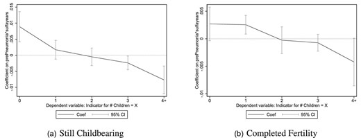
Estimated effects of pneumonia mortality decline on the fertility distribution. This figure displays the coefficients and |$95\%$| confidence intervals around coefficients on the variable |${ prePneumonia}\ast { sulfayears}$| in a set of five separate OLS regressions, where the dependent variables in these regressions are indicator variables for having no children in the household, exactly one child, exactly two children, exactly three children, and four or more children, based on the net fertility measure.
Completed Fertility.
We now discuss fertility impacts on women who were aged 40–50 at census and had thus plausibly completed their fertility. We present results using the same net fertility measure as used in the hazard model, which relies on counts of children living at home, for which we impose an upper limit of age at census of 50 to reduce the omission of children who have left home.44
The pattern of results is similar to that documented so far: Pneumonia mortality decline is associated with a significant decline in fertility on both the extensive and intensive margins. In particular, an interquartile decline in pneumonia mortality (0.26), evaluated at the average number of reproductive years of exposure to sulfa drugs (14.9), led to 0.11 fewer children for the average woman, which is 5.7% of the pre-sulfa baseline mean, and a 1.4 percentage point increase in the probability of being childless, a 5.0% increase from baseline (panel B, Table 3).
Comparing estimates for net fertility among women age 40–50 at enumeration with the estimates for fertility of women of childbearing age (18–40) from the preceding section (comparing panels A and B in Table 3), the coefficients for women who have completed fertility are consistently smaller than the coefficients for women who are of childbearing age. This is also evident when comparing changes in the distribution of incomplete and completed fertility (Figure 7). The estimates suggest that two-thirds of the estimated impact of pneumonia mortality on childlessness in the childbearing-age sample is compensated delay, and that one-third is a rise in permanent childlessness; the latter will likely incorporate both a decline in target fertility and uncompensated fertility delay that may arise from biological decline in fecundity or from failure to find a marital match, as modeled in Section 4.
5.4. Results: Labor Market and Education Outcomes
Panel A of Table 5 shows that reductions in pneumonia mortality led to improved labor market outcomes for women by every indicator used, other than income.45 A decline in pneumonia mortality corresponding to an interquartile shift in the distribution, for a woman with the mean exposure to sulfa drugs in the estimating sample (18.3 years), is estimated to have increased the probability of being in the labor force by 2.6 percentage points and the probability of being employed of 2.8 percentage points. The average labor force participation rate (employment rate) in this sample is 37.1% (35.1%), so this increase is 7.0% (8.0%) of the baseline rate. This is of broadly similar magnitude to our estimate of the increase in the share of childless women.46
Total gross fertility (number of children) as a function of sulfa exposure.
| (1) | (2) | (3) | |
|---|---|---|---|
| # Children | # Children |${\vert }$| Children |$>$|0 | Childless | |
| |${prePneumonia}\ast {sulfayears}$| | |$-0.0209^{*}$| | |$-0.0187^{*}$| | 0.0021|$^{**}$| |
| (0.0118) | (0.0106) | (0.0009) | |
| N | 518,933 | 421,983 | 518,933 |
| Mean | 2.5750 | 3.1660 | 0.1866 |
Notes: These regressions are comparable to panel B of Table 3, except that fertility outcomes are measured based on gross fertility (total number of live births). The sample contains women aged 40–50 at census. *denotes p-value < 0.1, **denotes p-value < 0.05, and ***denotes p-value < 0.01.
Labor market and marriage market outcomes as a function of sulfa exposure.
| (1) | (2) | (3) | (4) | (5) | |
|---|---|---|---|---|---|
| A: Labor market outcomes | Working | In labor force | H–W SEI | Personal income | Hours worked |
| |${prePneumonia}\ast {sulfayears}$| | 0.0058|$^{***}$| | 0.0055|$^{***}$| | 0.1991|$^{**}$| | 7.3736 | 0.2421|$^{***}$| |
| (0.0017) | (0.0018) | (0.0771) | (15.4010) | (0.0652) | |
| N | 727,398 | 727,398 | 517,857 | 306,280 | 727,398 |
| Mean | 0.3510 | 0.3710 | 14.4093 | 1505.191 | 12.8097 |
| (1) | (2) | (3) | |||
| B: Marriage market outcomes | Currently married | Ever married | Age at 1st marriage | ||
| |${prePneumonia}\ast {sulfayears}$| | |$-0.0023^{*}$| | -0.0032|$^{**}$| | 0.0021 | ||
| (0.0012) | (0.0012) | (0.0243) | |||
| N | 494,437 | 727,398 | 116,632 | ||
| Mean | 0.7258 | 0.8284 | 20.6429 |
Notes: |${prePneumonia}\ast {sulfayears}$| is the average state-level pneumonia mortality rate between 1930 and 1936, interacted with the number of fertile years (aged 15–40) that a woman was exposed to sulfa drugs. These are OLS regressions with standard errors (in parentheses) clustered at the state of birth level. Panel A: The dependent variables are: (1) a dummy variable equal to 1 if the woman reports working at the time of the census, and 0 otherwise; (2) a dummy variable equal to 1 if the woman is in the labor force, and 0 otherwise; (3) the Hauser–Warren Socioeconomic Index, based on occupation, available for the 1950+ censuses; (4) the U.S. Dollar amount of personal earnings in the past year, available for the 1950+ censuses; (5) hours worked in the past week, converted from intervalled data to a continuous measure using the midpoint of each interval. We find similar estimated effects of sulfa exposure on other measures of occupational score, including occscore (coefficient(standard error) 0.0775(0.0473) on |${prePneumonia}\ast {sulfayears}$|), and the Duncan socioeconomic score (coefficient(standard error) 0.1512(0.0893)). Panel B: The dependent variables are: (1) a dummy variable equal to 1 if the woman is married at the time of the census, and 0 otherwise; (2) a dummy variable equal to 1 if the woman has ever married in her lifetime, and 0 otherwise; (3) the age at first marriage for women who have ever married. The cohorts in this panel were born in the years 1900–1931 for columns (1) and (3) (1893–1931 for column (2)) and are drawn from the 1940, 1950, 1960, and 1970 U.S. decennial population censuses. *denotes p-value < 0.1, **denotes p-value < 0.05, and ***denotes p-value < 0.01.
The same decline in pneumonia mortality led to an increase in the occupation-based socioeconomic index of 6.6% relative to the baseline index score of 14.4, suggesting that women exposed to sulfa drugs had better careers, consistent with the mechanism in Section 4. We obtain similar results when considering other occupational scores, including occscore and the Duncan socioeconomic index. Pneumonia mortality decline increased weekly working hours by 1.15 hours, or 9% of the baseline mean, which implies an annual increase of 13.8 hours for the sample average of 12 working weeks per year.47 Although the coefficient on pneumonia mortality decline is positive for personal income, it is imprecisely estimated.
The Joint Probability of Childlessness and Labor Force Participation.
Thus far, we have demonstrated, using independent reduced form equations, that the sulfa-led reduction in pneumonia mortality led to lower total fertility, higher childlessness and higher rates of labor force participation, employment, working hours, and occupational quality among women. Tabulating labor market outcomes by childlessness status (Online Appendix Table A.3) shows that childless women were 34 percentage points more likely to be in the labor force, worked 12 additional hours per week, earned over $1,000 more per year and had higher occupational scores than women who were mothers. In order to provide robust evidence that these choices are linked and, in particular, that the same women that respond with higher childlessness respond with higher labor force participation, we estimate the impact of sulfa-led mortality declines on the joint probability of being childless and being in the labor force (Table 6).
The joint probability of labor force participation and childlessness as a function of sulfa exposure.
| (1) | (2) | (3) | (4) | |
|---|---|---|---|---|
| In labor force | Not in labor force | |||
| Childless | Not childless | Childless | Not childless | |
| |${prePneumonia}\ast {sulfayears}$| | 0.0056|$^{***}$| | |$-0.0001$| | 0.0013 | |$-0.0068^{***}$| |
| (0.0017) | (0.0010) | (0.0012) | (0.0019) | |
| N | 727,398 | 727,398 | 727,398 | 727,398 |
| Mean | 0.205 | 0.166 | 0.140 | 0.489 |
Notes: The dependent variables are dummy variables for the four possible combinations of labor force participation status and childlessness status (based on net fertility) at the time of census enumeration, that is, each woman will fall into one of these four categories and will have a 1 for that dummy variable and a 0 for the other three. These are OLS regressions with standard errors (in parentheses) clustered at the state of birth level. The sample contains women age 18–50 at census. *denotes p-value < 0.1, **denotes p-value < 0.05, and ***denotes p-value < 0.01.
Reductions in pneumonia mortality increased the probability that women were both working and childless by 2.7 percentage points (13% of the baseline probability of 20.5%); see column (1). The probability of not being in the labor force and having children declined by 3.2 percentage points, or 6.5% (column (4)), while the probability of not working and being childless, or working and having children, did not change. We cannot reject that the coefficients in columns (1) and (4) are of the same magnitude but opposite sign, which indicates that among women experiencing greater declines in pneumonia mortality, stay-at-home mothers became less common, while working women without children became more common.
Education Outcomes.
To complement the results on labor market outcomes, in Online Appendix Table C.8, we report estimates of the effect of sulfa-induced mortality decline on education choices. Note that the fact that we consider women who were already of childbearing age in 1937 in our main analysis means that many of these women will have already completed their education. (These were 74% in the birth timing sample and 68% in the completed fertility sample.) We nevertheless investigated education acquisition by creating a sample of women aged 15–25 in 1937 and defining exposure to sulfa drugs as being aged 20 or under in 1937, as college completion typically occurred in the early 20s. We estimate a 5.4 percentage point increase in the probability of high school completion, relative to a baseline mean of 19.2% for this subsample of women. We find no effect on the rate of college completion, which is consistent with Goldin, Katz, and Kuziemko (2006), who discuss the timing of the expansion of college education, and that this occurred later, among the children (rather than the mothers) of the sulfa cohorts.
5.5. Results: Marriage Market Outcomes
Fertility delay and investment in the labor market is likely to have repercussions for the marriage market, and this mechanism is also discussed in an extension to the model in Section 4. We explore the impact of sulfa exposure on current marital status and age at first marriage for childbearing women (aged 18–40 at census) to capture any delay in marriage that may have mirrored fertility delay, and ever married status for women aged 18–50 at census.48 The results are in panel B of Table 5: Reductions in pneumonia mortality led to both postponement of marriage and a decline in marriage entry. A reduction in pneumonia mortality of the size of an interquartile shift is estimated to have reduced the probability of women ever having married by 1.4 percentage points (1.65% of baseline mean), and, among still childbearing women, to have reduced the probability of being married at the time of the census by 1 percentage point (1.5%).
Baudin, de la Croix, and Gobbi (2020) propose a model of childlessness in which marriage is a key pathway.49 In line with their predictions, we find that child mortality decline is associated with lower chances of having ever married, alongside an increase in childlessness. However, the coefficients indicate small effects relative to the labor market responses, suggesting that marriage was one important margin of response, but that labor force participation, rather than marriage, was the main mediator of impacts of child mortality decline on childlessness in our setting.
5.6. Robustness Checks
This section discussed specification checks on the later life outcomes. Many of the checks presented here are motivated and described in Section 3, so we discuss them briefly and point to the results. We conduct all robustness checks on the net and gross fertility measures, to provide firm evidence that our results are not driven by our choice of fertility measure.
Nonparametric Patterns.
To corroborate our results, we show that similar patterns emerge in a nonparametric specification that compares average outcomes over time in states that had above versus below median pneumonia mortality in the pre-sulfa era. Online Appendix Figure C.9 shows that in the 1950, 1960, and 1970 censuses, women in above-median mortality states who experienced larger declines in child mortality exhibited increases in childlessness alongside lower intensive margin fertility, relative to women in below-median states. In the pre-sulfa years (1930 census and before), the trends in fertility outcomes look similar across these two groups of states. Similarly, while labor force participation rates converge until 1940, they diverge after that, with women in above-median mortality states participating in the labor force in greater numbers. Finally, marriage rates evolve in a parallel fashion up until 1940, after which the marriage rates of women in above-median mortality states fall and remain lower than those of women in below-median mortality states. These patterns are consistent with the causal estimates.
Omitted Trends.
The birth timing results are identified on the assumption that the event of the introduction of sulfa drugs disrupts women’s birth profiles. In contrast to most studies of fertility, we provide estimates both for birth probabilities around the event and for the eventual number of children. By their nature, models of end-line fertility rest on stronger identifying assumptions than models of fertility behavior on either side of an event. Nevertheless, the results stand up to a number of checks. There is no natural event study but we provide a visual depiction of changes in the outcome against variation in exposure. As exposure is a function of birth cohort, we interact birth cohort “bins” with baseline pneumonia mortality, and plot the coefficients on the interaction terms in Online Appendix Figure C.8. The omitted case is 0 years of exposure. Panels A and B confirm the main results that childlessness was more likely with higher years of exposure, and that the total number of children was smaller. Panel C confirms hat women with higher years of exposure were more likely to be in work.
Panel B in Online Appendix Tables C.1, C.2, and C.3 adds controls for a full set of cohort * census region fixed effects, and the coefficients are stable even in this more demanding specification. We display sensitivity of the coefficients to varying the controls included in Online Appendix Table C.4. We augment the rich set of state-level controls for disease environment, economic conditions and surveillance quality with occupation structure. We include the state level occupational distribution of women in 1930 interacted with |${sulfayears}$| (panel A, Online Appendix Tables C.9, C.10, and C.11).
We address the possible role of mean reversion by controlling for the state-level pre-sulfa average value of the outcome variable (panel D, Tables C.5–C.7). We estimate impacts of a “placebo” intervention using an approach similar to that in Aaronson, Lange, and Mazumder (2014). This directly addresses concerns over omitted long-run trends in the stock model. We use data on individual outcomes in the 1910–1930 censuses, selected so that the outcomes were realized before the invention of sulfa drugs, and we create a placebo intervention 40 years previous to the true year (i.e. in 1897 rather than 1937), so that we have sufficient variation in placebo sulfa exposure in the census data. We then estimate the baseline specification of the stock model. The results in panel A of Online Appendix Tables C.13–C.15 show that the coefficients on pneumonia mortality are small and insignificant.
Since individual years of exposure evolve linearly as a function of birth cohort, we redefine the exposure variables to be binary, comparing the fully exposed with the unexposed, and omitting partially exposed women from the sample. The results are consistent with the main findings (Online Appendix Table C.21).
To provide evidence that our results do not capture differences in trends between regions of the United States, we show estimates omitting the mountain west and deep south states in turn (Online Appendix Tables C.13–C.15, panels B and C). We check that our conclusions are unchanged by including migrating women and instrumenting their mortality decline exposure in their residence state with their birth state (Online Appendix Tables C.16–C.18). We also check that the coefficients on pneumonia mortality decline are not sensitive to omitting maternal mortality decline (panel B in Online Appendix Tables C.26–C.28).
Coincident Events.
As with the birth timing model, we account for events occurring around the time of sulfa drug intervention: WW2, the Great Depression and New Deal program, and the Dust Bowl. To account for WW2, in the stock model, we control for state-level troop deployment, obtained from Goldin and Olivetti (2013), interacted with individual exposure to the war, measured as the number of fertile years of the woman from 1942 onwards. Our findings are essentially unchanged (panel B, Tables C.5–C.7). We interact New Deal spending (Fishback, Kantor, and Wallis 2003) with sulfa exposure (|${sulfayears}$| in the stock model). The coefficients of interest are robust to this (panel A, Online Appendix Table C.5 for fertility outcomes, and panel A, Online Appendix Tables C.6 and C.7, for labor and marriage market outcomes). Finally, we estimate a specification where the Dust Bowl states are omitted (panel C, Tables C.5–C.7).
Measurement Issues with Fertility.
To address the concern that the net fertility measure misses children who have left home, we show similar estimates in three variants. First, we estimate results using gross fertility, defined by a census question on total live births. These estimates, in Table 4, show 0.081 fewer total births for the average woman, which is 3% of the baseline mean, and a 0.8 percentage point increase in the probability of being childless, which is 4.3% of the baseline mean. The estimates are very similar to those for net fertility.
Second, we follow Aaronson, Lange, and Mazumder (2014) and in our measures of net fertility only include children aged below 10 (panel B of Online Appendix Table C.13). A further threat to inference with net fertility arises if the age at which children leave home is correlated with state level baseline pneumonia or maternal mortality. Although this should be absorbed by state fixed effects, the results are similar when considering net fertility among different age groups of women at census, focusing on younger women where children are less likely to have moved out (see Online Appendix C).
Child Versus Adult Health.
We report results when using the child pneumonia mortality rate instead of the all-age rate in Online Appendix Table B.3. The birth timing coefficient is attenuated, but the longer run life course outcome results hold.50 In the main analysis, which uses the all-age rate, it is possible that an improvement in women’s health ensuing from the advent of antibiotics contributed to the identified changes. To investigate this further, we control for cause-specific female mortality rates or cause- and age-specific adult mortality rates.51 Panel A in Online Appendix Tables C.1–C.3 replaces all-age all-sex mortality rates from heart disease, cancer, and TB with comparable ones among women only, and also adds diarrhea mortality among women above age 2. We include as a control adult (age 20–64), all-sex mortality rates for heart disease, cancer, TB, and mortality interacted with |${sulfayears}$| in panel B, Online Appendix Tables C.9–C.11, also adding diarrhea mortality among all individuals above age 2. The estimated coefficients for total fertility and the labor market are robust to this.
More broadly, it is unlikely that women’s health drives the entire impact because all-age pneumonia mortality occured largely among children (see Figure 1). Child mortality from pneumonia was 11.73 per 1,000 in the pre-antibiotic years, approximately 29 times as large as the adult rate of 0.4 per 1,000 people. After antibiotics arrived, the child pneumonia mortality rate exhibited the largest drop and it is what drives the first stage (Figure 2). The identified impacts are somewhat too large to be explained solely by a decline in adult mortality. For instance, we found a 6.9% reduction in birth probability in the immediate aftermath of the new antibiotics, a 13% increase in childlessness at age 40, and a 7.0% increase in labor force participation. These could reflect responses to improvements in women’s health only if women “over-responded” to these improvements.
Other Checks.
Online Appendix C discusses and shows that our estimates are robust to the following further checks: alternative age-at-census sample definitions; adjustment of standard errors for multiple hypothesis testing; and exclusion of outlier states.
6. Broader Relevance: Long-Run Patterns in the Data
We have shown that in response to declines in pneumonia mortality, women had fewer children and were more likely to be childless. They also had higher labor force participation and lower marriage rates. To complement these findings from the context of sulfa drugs, we demonstrate that these patterns are evident more broadly, in the raw data for the United States in 1930, as well as in contemporary data across African countries.
Figure 8 plots the cross-sectional correlation across U.S. states in 1930 of pneumonia mortality with each of childlessness and total fertility. Childlessness is negatively correlated with pneumonia mortality, while total fertility is positively correlated with it. The Figure also shows scatter plots of labor force participation and marital status against child mortality. Labor force participation is inversely correlated with child mortality (though less pronounced than childlessness), while marriage is positively correlated, consistent with our causal estimates.
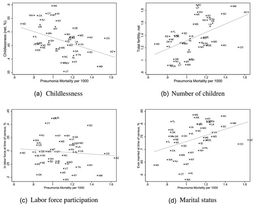
Relationship between pneumonia mortality and fertility, labor supply, and marriage in 1930 across U.S. States. These figures show the relationship between the average state-level outcomes of women in the different U.S. states in the 1930 census and the 1930–1936 average pneumonia mortality rates in these states. Fertility outcomes are defined based on net fertility and other outcomes are as used in the main analysis. The sample includes all women aged 18–50 at the time of the census.
Turning to contemporary data, Figure 9 plots the cross-country relationship between fertility, labor supply, and marriage and infant mortality (from all causes), across African countries in 2015. Similar to the early 20th century data from the United States, these contemporary data show a positive correlation of infant mortality with both total fertility and ever married rates, and a negative correlation of infant mortality with childlessness and labor force participation. These figures illustrate that the effects of child mortality decline that we document using the invention of sulfa drugs can be seen as broad correlational patterns in different time periods and different settings.
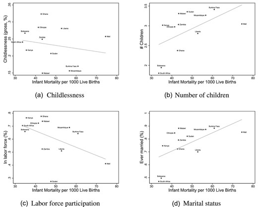
Relationship between infant mortality and fertility, labor supply, and marriage in 2015 across African countries. These figures show the relationship between the average country-level outcomes of women in different African countries and the infant mortality rate in these countries. The source of the fertility, labor market and marriage market data is the Integrated Public Use Microdata Series International Database: All countries for which Integrated Public Use Microdata Series data was available in 2000 or later are included, and all women aged 18–50 at the time of the census are included. We chose the census year closest to 2015 for each country. The mortality data are for 2015 and these data are sourced from UNESCO. Fertility is measured using the gross fertility measure (total births); childlessness is zero births.
7. Conclusions
The analysis produces two striking findings. First, a decline in child mortality (driven by pneumonia decline) led to fertility delay, a reduction in overall fertility, with fewer women having three or more children, and an increase in childlessness. Second, the decline in pneumonia mortality was associated with a higher propensity to work, higher occupational scores, and a lower probability of having ever married. We argue that the two findings are linked, namely, that child mortality decline made it rational to delay fertility, and that this led to the changes in labor market and marriage outcomes that we document.
Reductions in child mortality allowed women to delay the start of fertility, reduced the total time that women had to spend childbearing, and also reduced their target number of children due to the effect of improvements in child health and child quality. They additionally reduced the time that women, being main caregivers, spent caring for sick children. Together, this will have allowed women more time for productive activities. For women in the labor market, positive shocks to wages, negative shocks to fecundity or fertility preferences, or inertia, can result in persistence of the childless state.
We outline a dynamic model of fertility and labor market choices that shows a greater propensity for fertility delay and labor force participation in response to a decline in child mortality, when the joint probability of promotion at work and child mortality is low. The estimated patterns are consistent with this theory, fairly large, and robustly determined. We also document these patterns in other time periods and contexts, namely in correlational plots in contemporary African data, and U.S. data before the invention of sulfa drugs.
The estimates are relevant to debates concerning the trade-off between career and family, the rise of female labor force participation, and to models of the demographic transition and economic growth. In richer countries, women are increasingly delaying fertility and often using assisted reproductive technologies as a fallback. In many poorer countries, child mortality is falling and women are modifying their fertility and labor force participation decisions. We provide new evidence on the drivers of childlessness and female labor force participation, and the need to consider fertility, labor market and marriage market choices in conjunction. No previous work appears to have proposed and tested the idea that child mortality decline may influence labor force participation and marriage decisions of women, by triggering fertility delay. In a recent paper heralding a new era in the economics of fertility, Doepke et al. (2022) highlight the importance of policies that allow women to combine careers with families; also see Bhalotra, Clarke, and Walther (2022) for related discussion. In contrast to a large literature on subsidized child care, we highlight the relevance of child health and survival in allowing women to participate in the economy and build careers.
Our findings are relevant for contemporary development policy. Although, there have been marked declines in child mortality in the last 25 years in response to worldwide mobilization and increasing investments in public health, there is limited causal evidence of fertility and labor market responses to these investments. Our findings suggest that investments in child mortality decline can contribute to the economic independence of women, where labor market opportunities are available. Women’s labor force participation and associated economic independence can lead to increased investments in children (Baranov et al. 2020; Lundberg, Pollak, and Wales 1997) and a reduction in domestic violence (Aizer 2010; Bhalotra et al. 2021).
Acknowledgments
This paper has benefited greatly from the comments of Paola Giuliano (the Editor), three referees, Sascha Becker, David de la Croix, Christian Dustmann, James Fenske, Casper Worm Hansen, Hamish Low, Omer Moav, Andrew Oswald, Erik Plug, Debraj Ray, Gabriella Santangelo, Uwe Sunde, Petra Thiemann, Vellore Arthi, Joachim Winter and seminar participants at Oxford, Copenhagen, Warwick, UCL, Royal Holloway, Amsterdam, Munich, Surrey, Norwegian School of Economics, Milan Cattolica, the European Central Bank, Cambridge, Tilburg, Essex, CERGE-EI, Sussex, Ca’Foscari, the IZA-SOLE Translatlantic Meeting of Labor Economists, the COSME Gender Economics workshop, the Prague Workshop on Gender and the Family in the Labor Market, the Public Health and Development workshop in Gothenburg, a workshop in Nuremberg, the SEHO meetings in Lisbon, and the European Economic Association meetings in Lisbon. The authors are grateful to Yuki Kimura and David Hollywood for research assistance. Sonia’s research time was partly funded by Economic and Social Research Council of the UK awards ES/L009153/1 and ES/S003681/1 to the Centre for Microsocial Change, Economic and Social Research Council of the UK award ESM010236-1 to the Human Rights, Big Data and Technology project at the Human Rights Centre in Essex, and contributions from the University of Warwick. Bhalotra is affiliated at CEPR, IEA,CAGE, and IZA. Walther is affiliated at IZA and CERGE-EI.
Footnotes
Four forces are likely to be at play here. First, the direct effect of more births surviving will lower replacement behavior in fertility. Second, it will tend to reduce hoarding behavior that arises because mortality is uncertain. Third, because declines in mortality are typically associated with declines in morbidity (and thus an improved child health endowment), there is an increase in the incentive to invest in child quality, which will tend to reduce the target (desired) number of children as long as the effect of a reduction in the price of child quantity does not dominate. Fourth, a decline in sickness rates and hence the need to care for sick children will also tend to release the time of women for labor market engagement. Evidence of replacement and hoarding effects is provided in Bhalotra and van Soest (2008) using data from India from a period with broadly similar exposure to infectious diseases including pneumonia.
They use a triple difference approach, modeling fertility of Black relative to White women in response to the Rosenwald program that created schools for Blacks in the 1920s.
Recent models of childlessness suggest that involuntary childlessness at the bottom of the education distribution arises from poverty, while childlessness at the upper end of the education distribution is voluntary, being driven by the opportunity cost of childbearing (Baudin, de la Croix, and Gobbi 2015; also see Aaronson, Lange, and Mazumder 2014 in relation to the opportunity cost mechanism).
In contrast to our findings, the pill had no impact on completed fertility at either margin (Ananat and Hungerman 2012). A possible explanation for this difference is that women in the antibiotic era were more likely to have to choose between career and family, while women in the pill era could more easily have both Goldin (2004) and Coles and Francesconi (2019).
The chemical structure of sulfonamide had previously been documented as part of a PhD thesis in the early 1900s. By the time it was established in the 1930s that it had antibacterial properties, the patent had expired and anyone was allowed to produce sulfonamide for commercial purposes.
Sulfa drugs also reduced mortality and morbidity from skin and soft tissue infections and meningitis (Jayachandran, Lleras-Muney, and Smith 2010). However, the incidence of these diseases was very low and they made insignificant contributions to mortality rates. For example, the all-age mortality rate from skin diseases in the United States was 1.8 per 1,000 in 1930, and from meningitis 2.1, compared with an all-cause infant mortality rate of 69 (Vital Statistics).
Following a tradition in the literature (Almond 2006; Bozzoli, Deaton, and Quintana-Domeque 2009), we assume that changes in mortality are a proxy for both mortality and morbidity, both of which improved due to the arrival of sulfa drugs. In this sense, mortality decline also captures improvements in the health of survivors.
The early 20th century in the United States featured the birth control movement, led by political radicals Emma Goldman, Mary Dennett, and Margaret Sanger, who argued the importance of birth control. The first birth control clinic was opened in 1916, but shut down, followed by a clinic in 1923, which was not shut down. These clinics were the precursor to Planned Parenthood.
The relationship between fertility control and career choices has been discussed in sociology (for example, see Wilkie 1981; Bloom and Trussell 1984; Lundquist et al. 2009; Hayford 2013). In particular, see Murray and Lagger (2001), who analyze this in the context of the United States demographic transition in the 19th century.
In 1936, a year before the introduction of sulfa drugs, Popenoe (1936) conducted a survey among students at the University of Southern California asking them to describe the history of all permanently childless couples that they knew. This shows that 22% of couples were believed to be childless due to the wife’s career, and 16% childless due to economic pressure, suggesting that fertility and labor market choices were linked during this period, even for married women.
Marriage bars were regulations that prevented married women from working (see Goldin 2006).
In all datasets, we restrict the sample to United States born women not residing in group quarters who are resident in their birth state at the time of the census. The latter limits bias that could arise due to migration; see Section 3.4 for robustness checks on migration.
The uptick in the combined influenza plus pneumonia mortality rate on account of an influenza epidemic in 1936 and 1937 results in the decline after 1937 being sharper, but some of this reflects reversion to the mean. Comparison of the post-1937 rates with the rates in 1930–1934 in the plot makes even clearer that mortality decline after 1937 was driven by the child mortality rate. In the analysis, we address the uptick in 1936 and 1937 by defining baseline rates as an average over 1930 and 1936, and we also provide a test of whether our estimates are driven by mean reversion.
For diarrhea, we use the mortality rate for children under the age of 2, given both data availability considerations and the fact that adults typically do not die of diarrheal infections. For other control diseases, we use the all-age rate.
For female labor force participation and literacy, we use the value in 1930 as values for other years are unavailable. In a robustness check, we also control for baseline occupational structure at the state level, to allow that women’s employment opportunities were restricted by the availability of occupation.
Although pre-intervention levels of pneumonia and maternal mortality are positively correlated, they also exhibit substantial independent variation across the U.S. states (see Figure C.5 in Online Appendix C), and Online Appendix Figure C.6. The parameter |$\alpha _{2}$| will reflect causal effects of maternal mortality decline on the birth probability.
Our focus on improvements in child health and survival is backed by evidence that children born after the antibiotic revolution had higher education and income, consistent with the introduction of antibiotics driving lower fertility and higher investments in child quality (Bhalotra and Venkataramani 2011).
Column (1) in Table 1 pools a woman’s births, and in so doing assumes independence across recurrent events. Standard errors are clustered at the state level, which allows for non-independence within mothers as, by construction, they do not move state. The extensive margin result in column (2) is robust to this concern, as the extensive margin has one event (the first birth).
Standardizing the logistic coefficients by the variance in the outcome variable yields coefficients that are directly comparable across samples, and shows that the negative effect of the reduction in pneumonia mortality on the extensive margin birth probability in column (2) is similar to the effect on the overall birth probability in column (1), and both are approximately three times the size of the effect on the intensive margin in column (3).
Occupational structure is calculated as the share of women employed in primary, secondary, or tertiary industries in the 1930 census, yielding three variables.
Specifically, we estimate variants of the regression:
where |${controlvar}$| are all the state-time varying controls in our main estimates. For compactness, we do not report these results but they are available on request from the authors.
The mountain states are Arizona, Colorado, Idaho, Montana, Nevada, New Mexico, Utah, and Wyoming. The deep south states are Louisiana, Mississippi, Alabama, Georgia, and South Carolina.
These were Nebraska, Kansas, Colorado, New Mexico, Oklahoma, and Texas.
When child mortality is high, gross fertility (children ever born to a woman) will overestimate surviving births. Measuring children living with the mother partially addresses this problem, but not entirely as children alive at the census date may subsequently die. The extent of overestimation will be correlated with pre-intervention pneumonia mortality, which is part of our exposure variable. Pneumonia mortality rates decline exponentially from birth to age 5, after which they flatten out. Therefore, the fact that we find similar estimates when restricting our measure of fertility to children aged below 10 and when including all surviving children, suggests that any survivorship bias is likely to play a limited role in our estimates.
The states entered the National Registration System at varying dates between 1915 and 1933 for birth registration, and between 1880 and 1933 for death registration. Upon entering the registration system, states typically engaged in a few years of “learning by doing”, resulting in continued improvements in death registration and cause ascertainment until vital registration systems fully matured. Thus, we may expect measurement error to have declined with years since entry to the national registration system. We analyse the first year in which a state had achieved both birth and death registration, but the results we display are similar if we analyse registration timing for birth and death separately.
These trends are not available separately for child and adult mortality. However, we found death certificate data for 1940 that allow us to demonstrate that the problem of ascertaining cause of death of children was significant (see Figure C.1).
For example, the symptoms of pneumonia are similar to the symptoms of influenza and other infectious, congenital, inflammatory, or allergic causes of infant respiratory distress. The problem is aggravated for young children because they cannot clearly describe their symptoms and, with their nascent immune systems, are more likely to have more than one infection at a time. The under-counting of births is a further issue as births represent the population at risk of child mortality.
In the baseline specification, these are included as all-age rates with the exception of diarrhea, which was for under-2s given that adults typically do not die of diarrhea and diarrhea is relatively straightforward to diagnose among children. In this check, we remove all-age mortality from malaria, heart disease, cancer, and TB, and replace it with its adult rate equivalent (age 20–64). We also add diarrhea mortality among the over-2s to complement the under-2s rate already in the baseline regression. These rates are for the year 1935 only, interacted with |$post$|.
These are deaths among all-age women from heart disease, cancer, TB, and diarrhea above age 2.
Adda et al. (2017) also study a model in which women choose fertility over the life cycle, which they use to quantify the career costs of fertility in an environment where child mortality and health is held constant. Our model makes a complementary contribution by providing a clear analysis of the effects of health shocks.
Different patterns of behavior are possible in models with a richer income process or dynamics beyond three periods. We show in the Online Appendix that these extensions have more complex solutions, but do not alter our main qualitative results.
By contrast, the marginal cost |$\left(p+\lambda \right)\left(1-\lambda \right)V_{1}\left(A\right)$| of delay is decreasing in |$\lambda$| for large values of |$\lambda$|. Intuitively, as |$\lambda \rightarrow 1$|, both pregnancies of a woman who chooses early fertility are likely to fail, so that the “insurance” value of starting early declines to 0.
For a discrete change in |$\lambda$|, this implies that there is an interval of women who will switch their behavior between delayed and early fertility.
For example, consider a model where the pre-promotion wage, which we set to 0 for simplicity, is |$y>0$|. No fertility in this model is optimal whenever |$A\le \underline{A}\left(\lambda \right)$|, which is implicitly defined by |$y=\left(1-\lambda \right)V_{1}\left(\underline{A}\left(\lambda \right)\right)$|. Moreover, |$\underline{A}\left(\lambda \right)$| is increasing in |$\lambda$|.
Women in this era primarily worked in teaching and typing jobs, where the probability of promotion was low (Goldin 2004).
Unlike the predictions of our model on the extensive margin, this prediction is also a feature of the standard quantity–quality model, in which women tend to substitute out of quantity and into quality after a beneficial health shock.
The oldest woman in this was 44 in 1937, and she was reproductive until 1933, and the youngest woman was six in 1937, so that she was reproductive from 1946 onwards. For example, the 1917 cohort will have turned 40 in 1957, so we find them in the 1960 census when looking at their completed fertility.
We have intentionally opted to select samples based on age at census enumeration, in order to compare outcomes during childbearing and after childbearing years. This means that there is a small difference between the cohorts analyzed across the childbearing and completed fertility samples. We have verified that our main results are very similar when we restrict the sample of each estimate to have exactly the same cohorts.
This includes women reporting 0 hours of work; focusing only on positive working hours, the average was 37.9.
Notice that when we use the sample of women of reproductive age at the time of the census in these later census files, |${sulfayears}_{j}$| may include future years: For example, a woman aged 33 at the time of the 1950 census who was 20 in 1937, would have 20 fertile sulfa years in total, of which 7 are in the future. If women make dynamic fertility choices, they care about their total exposure to sulfa drugs, and not only their past exposure.
A number of recent studies suggest that including unit-specific trends can either exacerbate biases inappropriately or washout treatment effects when the evolution of these effects increases over time (or as in our case, with increasing cohort exposure); see, for example, Young and Gary (2011), Bhuller et al. (2013), and Goodman-Bacon (2021).
For some of these women, a disproportionate share of whom are younger and hence sulfa-treated during their reproductive years, fertility is right-truncated. This will be captured by fixed effects for the woman’s age, which we consistently include.
We will under-estimate fertility counts because some of the older children will have left home. Since older women in the sample will have had fewer years of sulfa exposure, if we selectively under-estimate their fertility, we will tend to under-estimate the coefficient of interest. The estimates we show are, by this criterion, conservative.
As the census asks women about their current labor market status, we include all women aged 18–50 at the time of the census, pooling both childbearing women and women aged 40–50, for whom we estimated effects on completed fertility. The results are very similar when widening the sample to include women aged up to 60, and narrowing the sample to women aged under 40 (see Online Appendix C).
If every additional childless woman worked (4.6 percentage points from the net fertility measure), the increase in labor force participation would be 12.4% of baseline labor force participation. Thus, 7% underlines the plausibility of the link between changes in childlessness and employment of women.
To put this in perspective, Bailey (2006) estimates an annual increase of 68 hours among cohorts with access to the birth control pill.
Estimates using alternative age-at-census samples are in Online Appendix C.
An important assumption in their model is that women have imperfect control over fertility. Child mortality acts to limit the fertility of women of low socioeconomic status. Thus, they argue, a reduction in child mortality will make less educated women less attractive on the marriage market, leading to increased childlessness and lower fertility. We thank David de la Croix for this insight.
The magnitudes of the coefficients are not directly comparable. A one-unit change in the all-age rate is roughly comparable to a eleven-unit change in the under-5 rate. The birth timing coefficient is estimated on smaller year to year changes than the other coefficients.
Ideally these rates would be for adult females rather than for all females but the age-specific mortality rates are not available by gender.
Notes
The editor in charge of this paper was Paola Giuliano.
