Optimal Taxation of Robots

Abstract

I study the optimal taxation of robots, other capital, and labor income. I show that it is optimal to distort robot adoption. The robot tax (or subsidy) exploits general-equilibrium effects to compress wages, which reduces income-tax distortions of labor supply, thereby raising welfare. In the calibrated model, when robots are expensive, a robot subsidy is optimal. As robots get cheaper, it becomes optimal to tax them. Yet, when reforming the status-quo tax system, most welfare gains can be achieved by adjusting the income tax. The additional gains from taxing robots differently from other equipment capital are close to zero.

1. Introduction

Public concern about the distributional consequences of automation is growing (see e.g. Brynjolfsson and McAfee 2014; Ford 2015; Frey, Berger, and Chen 2018). It is feared that the “rise of the robots” is going to disrupt the labor market and will lead to extreme income inequality. These concerns have raised the question of how redistributive policy should respond to automation. Some policymakers and thought leaders have suggested a “tax on robots”.^1,2 Is this a good idea? I show that based on optimal tax theory, robot adoption should be distorted. Yet, I find that rising inequality due to widespread robot adoption does not call for ever higher robot taxes. Instead, the robot tax (or subsidy) is small and should eventually go toward zero, while labor-income taxes should become more progressive. Moreover, reforming robot taxation yields only small welfare gains. However, if taxes on labor income cannot be adjusted (e.g. for political-economy reasons), robot taxation can partly compensate for suboptimal labor taxes.

In a tax system in which taxes on robots, other capital, and labor income can be set optimally, the robot tax exploits general-equilibrium effects to compress the wage distribution. Wage compression makes it less distortionary to tax income, which allows for more redistribution and raises welfare. If robots primarily substitute for routine labor at medium incomes, a tax on robots decreases wage inequality at the top of the wage distribution but raises inequality at the bottom. These counteracting effects on inequality make the sign of the optimal robot tax ambiguous.

Quantitatively, in the US, robots should initially be subsidized at a rate of about 0.5%. When robots get cheaper and are more widely adopted, wages in routine occupations come under pressure, and inequality rises. It then becomes optimal to tax robots at rates of up to 1%, which is close to the status-quo tax on equipment capital of 1.55%. Eventually, the efficiency costs of taxing robots weigh more heavily than the redistributive gains and the optimal robot tax decreases. At the same time, optimal income taxes should become more progressive. In fact, when reforming the status-quo tax system, most welfare gains can be achieved by adjusting labor taxes, while the welfare gains of reforming robot taxation are close to zero. Intuitively, direct redistribution with income taxes is more effective than indirect redistribution with robot taxes. However, if a labor-tax reform is not feasible, adjusting the robot tax can lead to substantial welfare gains. In this case, the robot tax partly compensates for the suboptimal labor taxes.

To reach these conclusions, I first build intuition by studying a simple model with discrete types. The full model then features within-occupation earnings heterogeneity and a participation margin. For the quantitative analysis, I calibrate the full model to the US economy.

The stylized model extends Stiglitz (1982) to three occupations: manual non-routine, routine, and cognitive non-routine. Output is produced by combining labor and robots. Crucially, wages of workers in different occupations are affected differently by robot adoption. The robot tax exploits this to compress wages to alleviate income-tax distortions of labor supply. Its sign is ambiguous as long as taxing robots increases wage inequality in some part of the wage distribution, while compressing wages in other parts.

What the sign and size of the optimal robot tax should be is ultimately a quantitative question. To address it, I extend the model to capture two important aspects of the data: Acemoglu and Restrepo (2020) find for the US that exposure to robots has differential effects along the wage distribution and that robots have an impact on employment (which differs by occupation). The full model thus features a continuous wage distribution as well as a participation margin, building on Rothschild and Scheuer (2013, 2014) and Jacquet, Lehmann, and Van der Linden (2013). Moreover, the full model accounts for equipment and structures capital in addition to robots. Despite these extensions, the optimal-robot-tax formula has a similar structure as in the stylized model. I exclude the option for individuals to switch occupation for three reasons: First, there is no strong evidence in Acemoglu and Restrepo (2020) of individuals switching occupation in response to robot adoption.³ Second, Acemoglu and Restrepo (2020) study a medium-run of 15 years in which large-scale occupational mobility is likely limited.⁴ This paper is also concerned with the medium run, and since automation is a cognitively biased technology, ruling out occupational mobility is a reasonable choice. Third, including both a participation and an occupational choice margin would make the model much less computationally tractable.⁵

I calibrate the full model to the US economy using wage and employment data from the Current Population Survey (CPS) as well as the evidence on robots and the labor market from Acemoglu and Restrepo (2020). Then, I compute the optimal tax system, which features taxes on the different types of capital, non-linear income taxes, and a transfer to non-participants. At initial robot prices, robots should be subsidized at a rate of about 0.5% to reduce inequality at the bottom of the wage distribution. As robots get cheaper and inequality rises, the optimal subsidy turns into a tax that peaks at 1% and then declines. In contrast, the optimal tax on equipment capital is always positive and larger than the robot tax, peaking at about 2% and then declining. Structures capital should not be taxed—a result echoing Slavík and Yazici (2014). As robots get cheaper, the optimal transfer to non-participants increases, and optimal income taxes should be adjusted by raising progressivity at higher incomes.

In the final step, I assess the welfare impact of reforming the status-quo tax system toward the optimum. I find that optimally setting non-linear income taxes, while keeping the status-quo for capital taxes, generates welfare gains between 1000 and 4000 USD per capita per year. Additional gains between 2 and 20 USD can be achieved by optimally setting taxes on capital—under the constraint that robots and equipment capital must be taxed at the same rate. Allowing for differential taxation of robots and equipment leads to almost no additional welfare gains. Only reforming taxes on robots, while leaving the rest of the tax system at its status-quo can generate welfare gains of a few hundred USD per capita.

This paper is organized as follows: Section 2 discusses the related literature. Section 3 sets up a simple model to build intuition. Section 4 characterizes the optimal robot tax in the full model. Section 5 studies the full model quantitatively. Section 6 concludes. Proofs for the simple model are contained in the Appendix. Proofs for the full model and additional material are collected in an Online Appendix.

2. Related Literature

This paper combines elements from Rothschild and Scheuer (2013, 2014), who extend and generalize Stiglitz (1982) by studying optimal non-linear income taxation with multi-dimensional heterogeneity and sectoral choice, and from Jacquet, Lehmann, and Van der Linden (2013) (see also Saez 2002), who study optimal taxation with intensive and extensive labor-supply responses.

A growing number of papers ask how taxes should respond to technological change. In parallel and independent work, Guerreiro, Rebelo, and Teles (2022) study the impact of robots on two types of workers—routine and non-routine—across generations, by introducing robots into a model similar to Stiglitz (1982), which is then embedded in an overlapping-generations framework. They show that it is optimal to tax robots as long as some tasks are still performed by routine workers. The rationale for taxing robots is the same as in this paper: compressing the wage distribution to reduce income-tax distortions of labor supply.⁶ In contrast to Guerreiro, Rebelo, and Teles (2022), I show that it can sometimes be optimal to subsidize robots. Moreover, I argue that even if robots should be taxed, taxing them differently from other equipment capital generates almost no welfare gains. I arrive at these conclusions by studying three instead of two occupations, and by conducting welfare analyses using a rich and carefully calibrated model. Studying three occupations better captures that workers in routine occupations are most affected by robots, while workers in manual and cognitive non-routine occupations are affected less.

Relatedly, Costinot and Werning (2022) ask how tax policy should respond to inequality driven by technology or trade if the set of policy instruments is restricted, such that production efficiency as in Diamond and Mirrlees (1971) is not optimal. As one application, they study the optimal tax on robots. Using a sufficient-statistics approach, Costinot and Werning (2022) find optimal taxes of very similar magnitude as this paper. My complementary structural approach allows me to study taxation of structures and equipment capital in addition to robots, and to analyze counterfactuals such as the impact of a drop in the robot price as well as various tax reforms.

Acemoglu, Manera, and Restrepo (2020) study a Ramsey problem in which the planner chooses optimal labor and capital taxes as well as the level of automation. They take into account labor market frictions, while abstracting from distributional effects, which is the focus of this paper. Schulz, Tsyvinski, and Werquin (2022) derive how a given tax system needs to be adjusted to compensate individuals for the distributional effects of, for example, trade or automation. In an application, they use the results from Acemoglu and Restrepo (2020) to investigate how individuals should be compensated for changes in income generated by the increased use of industrial robots. In contrast to this paper, Schulz, Tsyvinski, and Werquin (2022) do not study optimal taxation. Other papers (Zhang 2019; Prettner and Strulik 2020; Gasteiger and Prettner 2022; Hémous and Olsen (2022) study the impact of taxing robots, taking a positive—rather than a normative—perspective.⁷

The implications of technological change for tax policy are also analyzed by Ales et al. (2015), who study a model in which individuals are assigned to tasks based on comparative advantage, by Jacobs and Thuemmel (2018, 2022), who study optimal tax and education policy under skill-biased technical change, and by Loebbing (2020), who studies the interplay of optimal income taxation and directed technical change, but none of these papers studies robot taxation.

A tax on robots violates production efficiency. This paper is thus related to the Production Efficiency Theorem (Diamond and Mirrlees 1971), which states that production decisions should not be distorted, provided that the government can tax all production factors—inputs and outputs—linearly and at different rates. This requirement is ambitious. Instead, Naito (1999), Saez (2004), Naito (2004), Jacobs (2015), Shourideh and Hosseini (2018), Guerreiro, Rebelo, and Teles (2022), and Costinot and Werning (2022) all study settings that feature fewer tax instruments than needed for achieving production efficiency. Similarly, in this paper, the set of tax instruments is too restricted for production efficiency to be optimal. In particular, income taxes may not be conditioned on occupation.^8,9

A recent empirical literature studies the impact of robots on the labor market.¹⁰ Using data on industrial robots from the International Federation of Robotics (IFR 2014), Acemoglu and Restrepo (2020) exploit variation in exposure to robots across US commuting zones to identify the causal effect of industrial robots on employment and wages between 1990 and 2007. I use their results to calibrate the full model. Other articles that study the impact of robots on labor markets are Graetz and Michaels (2018) for a panel of 17 countries, Dauth et al. (2019) for Germany, Acemoglu, Lelarge, and Restrepo (2020) for France, and Barth et al. (2020) for Norway.

Robots are a specific type of capital. Most arguments for taxing capital do not depend on the differential impact of capital on wages, making them orthogonal to the reason for robot taxation in this paper. An exception is Slavík and Yazici (2014), who, in a dynamic setting, give a similar argument for taxing equipment capital as this paper does for taxing robots.¹¹ Rather than focusing on dynamic aspects, I model the cross-sectional labor market in detail, allowing for within-group earnings heterogeneity and including a participation margin, both of which are not present in Slavík and Yazici (2014) but are important in the context of robot taxation.

3. Simple Model to Build Intuition

To build intuition, I first discuss a simple model that features discrete types and abstracts from participation choice. The model extends Stiglitz (1982) to three sectors (or occupations) and features endogenous wages.

3.1. Setup

3.1.1. Workers, Occupations and Preferences

There are three types of workers |$i\in \left\lbrace M,R,C\right\rbrace $| with corresponding mass |$f_{i}$|⁠. A worker’s type reflects his occupation, where M refers to an occupation that requires manual non-routine labor, R refers to an occupation requiring routine labor, and C denotes a cognitive non-routine occupation. The distinction between routine and non-routine occupations is motivated by the empirical literature, which has established that in recent decades technology has substituted for routine work, and has complemented non-routine work (see e.g. Autor et al. 2003). Moreover, the literature on labor market polarization suggests distinguishing between low-skilled and high-skilled non-routine occupations (see e.g. Cortes 2016; Cortes, Jaimovich, and Siu 2017). Workers derive utility from consumption c and disutility from labor supply |$\ell$| according to the quasi-linear utility function

$$\begin{eqnarray} U\left(c,\ell \right)\equiv c-\frac{\ell ^{1+\frac{1}{\varepsilon }}}{1+\frac{1}{\varepsilon }}, \end{eqnarray}$$

(1)

where |$\varepsilon$| is the labor-supply elasticity. Denote by |$w_{i}$| the wage earned by an individual of type i. The government levies a non-linear income tax |$T\left(y\right)$| on gross labor income |$y_{i}=w_{i}\ell _{i}$|⁠. Taking the wage and income tax schedule as given, a worker of type i maximizes utility (1) subject to the budget constraint

$$\begin{eqnarray} c_{i}\le w_{i}\ell _{i}-T\left(w_{i}\ell _{i}\right). \end{eqnarray}$$

(2)

3.1.2. Technology

Denote by |$\boldsymbol {L}\equiv \left(L_{M},L_{R},L_{C}\right)$| the vector of aggregate labor supplies with |$L_{i}=f_{i}\ell _{i}$| for all i. Let |$K_{B}$| denote robots. The final good is produced by a representative firm according to a constant-returns-to-scale technology |$Y\left(\boldsymbol {L},K_{B}\right)$|⁠. The firm maximizes profits by choosing the amount of aggregate labor of each type i and the number of robots, taking wages |$w_{i}$| and the price of robots |$p_{B}$| as given. Normalizing the price of the final good to one, the firm’s profit maximization problem is

$$\begin{eqnarray} \max _{\boldsymbol {L},K_{B}}\ Y\left(\boldsymbol {L},K_{B}\right)-\sum _{i}w_{i}L_{i}-p_{B}K_{B}. \end{eqnarray}$$

(3)

Denote the marginal products as

$$\begin{eqnarray} Y_{i}\left(\boldsymbol {L},K_{B}\right)\equiv \frac{\partial Y\left(\boldsymbol {L},K_{B}\right)}{\partial L_{i}}\ \forall i,\ Y_{B}\left(\boldsymbol {L},K_{B}\right)\equiv \frac{\partial Y\left(\boldsymbol {L},K_{B}\right)}{\partial K_{B}}. \end{eqnarray}$$

(4)

In equilibrium, we have |$w_{i}\left(\boldsymbol {L},K_{B}\right)=Y_{i}\left(\boldsymbol {L},K_{B}\right)\ \forall i$| and |$p_{B}=Y_{B}\left(\boldsymbol {L},K_{B}\right)$|⁠. I assume in this section that robots are better substitutes for routine work than for non-routine work.

Assumption 1.

A marginal increase in the number of robots raises the marginal product of non-routine labor relative to routine labor,¹² that is,

$$\begin{eqnarray} \frac{\partial }{\partial K_{B}}\left(\frac{Y_{M}\left(\boldsymbol {L},K_{B}\right)}{Y_{R}\left(\boldsymbol {L},K_{B}\right)}\right)>0,\ \frac{\partial }{\partial K_{B}}\left(\frac{Y_{C}\left(\boldsymbol {L},K_{B}\right)}{Y_{R}\left(\boldsymbol {L},K_{B}\right)}\right)>0. \end{eqnarray}$$

Due to constant returns to scale, equilibrium profits are zero and robot ownership is irrelevant. Robots are produced linearly with the final good, according to

$$\begin{eqnarray} K_{B}\left(x\right)=\frac{1}{q_{B}}x, \end{eqnarray}$$

(5)

where x is the amount of the final good allocated to the production of robots and |$1/q_{B}$| is the marginal rate of transformation between robots and the consumption good. In the absence of taxes, we have |$p_{B}=q_{B}$| in equilibrium. Later, when taxes drive a wedge between |$p_{B}$| and |$q_{B}$|⁠, I refer to |$q_{B}$| as the producer price of robots and to |$p_{B}$| as the user price of robots.

3.1.3. Government and Tax Instruments

There is a benevolent government whose objective is to maximize social welfare

$$\begin{eqnarray} f_{M}\psi _{M}V_{M}+f_{R}\psi _{R}V_{R}+f_{C}\psi _{C}V_{C}, \end{eqnarray}$$

(6)

with |$\psi _{i}$| the Pareto weight attached to workers of type i, where the weights satisfy |$\sum f_{i}\psi _{i}=1$|⁠, and |$V_{i}\equiv U\left(c_{i},\ell _{i}\right)$| are indirect utilities. While the government is aware of the structure of the economy, it cannot observe an individual’s occupation. This assumption is satisfied by real-world tax systems, which also do not condition taxes on occupation, for example, because enforcement may be difficult. However, the government can observe individual income and consumption, as well as the value of robots purchased by the final-goods producer. Accordingly, I assume that the government has access to two tax instruments: a non-linear income tax |$T\left(y\right)$| and a tax on the value of robots |$t_{B}$|⁠.¹³ With the robot tax, the user price of robots is |$p_{B}=\left(1+t_{B}\right)q_{B}$|⁠. While throughout this paper I refer to |$t_{B}$| as a tax, I highlight that |$t_{B}$| may be negative, and may thus be a subsidy. The government faces the budget constraint

$$\begin{eqnarray} f_{M}T\left(y_{M}\right)+f_{R}T\left(y_{R}\right)+f_{C}T\left(y_{C}\right)+t_{B}q_{B}K_{B}=0, \end{eqnarray}$$

(7)

stating that by raising tax revenue with the income tax and the robot tax, it must break even. Introducing an exogenous revenue requirement does not change the analysis.

3.2. Optimal Policy

The government chooses tax instruments |$T\left(\cdot \right)$| and |$t_{B}$| to maximize social welfare (6) subject to the budget constraint (7). I first solve for the optimal allocation from a mechanism design problem. Afterward, prices and optimal taxes that decentralize the allocation are determined.¹⁴

The allocation must induce workers to truthfully report their type and thus needs to be incentive compatible. Since there is no heterogeneity of types within occupations, the only way in which workers can imitate one another is by mimicking the incomes of workers in other occupations. For now, I assume that the primitives of the model are such that |$w_{C}>w_{R}>w_{M}$|⁠. Moreover, I limit attention to those cases in which only the downward adjacent incentive constraints may be binding, while all other incentive constraints are slack. This case is the relevant one for gaining intuition, which carries over to the continuous-type model.¹⁵ To induce a cognitive worker to truthfully report his type, the following must hold:

$$\begin{eqnarray} V_{C}\ge U\left(c\left(V_{R},\ell _{R}\right),\ell _{R}\frac{w_{R}\left(\boldsymbol {L},K_{B}\right)}{w_{C}\left(\boldsymbol {L},K_{B}\right)}\right), \end{eqnarray}$$

(8)

where |$\ell _{R}\frac{w_{R}}{w_{C}}$| is the amount of labor that a cognitive worker needs to supply to mimic the income of a routine worker. Similarly, a routine worker has to be prevented from mimicking the income of manual workers, and thus

$$\begin{eqnarray} V_{R}\ge U\left(c\left(V_{M},\ell _{M}\right),\ell _{M}\frac{w_{M}\left(\boldsymbol {L},K_{B}\right)}{w_{R}\left(\boldsymbol {L},K_{B}\right)}\right). \end{eqnarray}$$

(9)

The mechanism design problem can be written as

$$\begin{eqnarray} \max _{\left\lbrace V_{i},\ell _{i}\right\rbrace _{i},\boldsymbol {L},K_{B}}\ \ f_{M}\psi _{M}V_{M}+f_{R}\psi _{R}V_{R}+f_{C}\psi _{C}V_{C} \end{eqnarray}$$

(10)

subject to the incentive constraints (8) and (9), the labor-market-clearing conditions

$$\begin{eqnarray} f_{i}\ell _{i}-L_{i}=0\ \forall i, \end{eqnarray}$$

(11)

and the resource constraint

$$\begin{eqnarray} \sum _{i}f_{i}\ell _{i}Y_{i}\left(\boldsymbol {L},K_{B}\right)+Y_{B}\left(\boldsymbol {L},K_{B}\right)K_{B}-\sum _{i}f_{i}c_{i}\left(V_{i},\ell _{i}\right)-q_{B}K_{B}=0. \end{eqnarray}$$

(12)

The first two terms in the resource constraint (12) sum to total output |$Y\left(\boldsymbol {L},K_{B}\right)$|⁠. The final term captures that |$x=q_{B}K_{B}$| units of the final good have to be used to produce |$K_{B}$| robots.

3.2.1. Optimal Robot Tax

To characterize the optimal robot tax, I use that at the optimum a change in robots may not lead to a change in welfare.

Theorem 1.

The optimal tax on robots is characterized by

$$\begin{eqnarray} t_{B}q_{B}K_{B}= \varepsilon _{w_{C}/w_{R},K_{B}}\ I_{CR}-\varepsilon _{w_{M}/w_{R},K_{B}}\ I_{RM} \end{eqnarray}$$

(13)

with elasticities of relative wages with respect to the number of robots defined as

$$\begin{eqnarray} \varepsilon _{w_{C}/w_{R},K_{B}}\equiv \frac{\partial \left(w_{C}/w_{R}\right)}{\partial K_{B}}\frac{K_{B}}{w_{C}/w_{R}}>0, \end{eqnarray}$$

(14)

$$\begin{eqnarray} \varepsilon _{w_{M}/w_{R},K_{B}}\equiv \frac{\partial \left(w_{M}/w_{R}\right)}{\partial K_{B}}\frac{K_{B}}{w_{M}/w_{R}}>0, \end{eqnarray}$$

(15)

and incentive effects

$$\begin{eqnarray} I_{CR}\equiv f_{C}\left(1-\psi _{C}\right)\left(\ell _{R}\frac{w_{R}}{w_{C}}\right)^{1+\frac{1}{\varepsilon }}, \end{eqnarray}$$

(16)

$$\begin{eqnarray} I_{RM}\equiv f_{M}\left(\psi _{M}-1\right)\left(\ell _{M}\frac{w_{M}}{w_{R}}\right)^{1+\frac{1}{\varepsilon }}. \end{eqnarray}$$

(17)

Proof.

See Appendix A.

At the optimum, robot-tax revenue, |$t_{B}q_{B}K_{B}$|⁠, is equal to the difference in incentive effects |$I_{CR}$| and |$I_{MR}$|⁠, weighted by the respective elasticities, |$\varepsilon _{w_{C}/w_{R},K_{B}}$| and |$\varepsilon _{w_{M}/w_{R},K_{B}}$|⁠. The elasticities capture the percentage increase in wages of non-routine workers relative to the wage of routine workers due to a 1% increase in the number of robots. By Assumption 1, an increase in robots raises the wage of non-routine workers relative to routine workers. As a consequence, |$\varepsilon _{w_{C}/w_{R},B}>0$| and |$\varepsilon _{w_{M}/w_{R},B}>0$|⁠. The incentive effects |$I_{CR}$| and |$I_{RM}$| capture how incentive constraints (8) and (9) are affected by a marginal increase in robots, and how this, in turn, affects welfare. With regular welfare weights (⁠|$\text{$\psi _{M}>1,$ }\psi _{C}<1$|⁠), the government wants to redistribute income from cognitive workers to routine workers, and from routine workers to manual workers.

I first focus on |$I_{CR}$|⁠. A robot tax discourages robot adoption. Since robots are more complementary to non-routine labor, |$w_{C}/w_{R}$| falls, as does inequality at the top of the wage distribution.¹⁶ The compressed wage gap makes it harder for cognitive workers to imitate the income of a routine worker. This helps redistribution and increases welfare, since routine labor needs to be distorted less to achieve the same level of redistribution as without the robot tax.

Turning to |$I_{RM},$| a robot tax increases the wage gap between routine and manual workers, leading to lower |$w_{M}/w_{R}$|⁠. This makes it easier for routine workers to imitate manual workers, making redistribution with income taxes more distortionary.

Taxing robots thus helps to redistribute income from cognitive to routine workers, but makes it harder to redistribute income from routine to manual workers. As a result, the sign of the optimal robot tax is ambiguous. If the first effect dominates, robots should be taxed; otherwise, they should be subsidized. In either case, it is optimal to distort the price of robots to make income redistribution less distortionary, thereby violating production efficiency (Diamond and Mirrlees 1971).

The ambiguous sign of the robot tax contrasts with Guerreiro, Rebelo, and Teles (2022), who argue that the robot tax should always be positive. This is due to Guerreiro, Rebelo, and Teles (2022) considering only two groups of workers: routine and non-routine. In their model, taxing robots unambiguously relaxes the single binding incentive constraint. My result highlights that aggregating workers into just two groups can mask the heterogeneous effects of robots on wages along the income distribution with consequences for the sign of the optimal robot tax.

4. Full Model

I now extend the model to continuous types and introduce a participation margin. As a result, the model features a continuous wage distribution and employment effects of robot adoption. I also include additional types of capital: equipment and structures.¹⁷ Taken together, these extensions make the model amenable to a realistic calibration.

4.1. Setup

4.1.1. Skill Heterogeneity

There is a unit mass of individuals. As before, each individual is assigned an occupation |$i\in \lbrace M,R,C\rbrace$|⁠, but now an individual’s skill |$\theta \in [\underline {\theta }_{i},\bar{\theta }_{i}]$| with |$\bar{\theta }_{i}>\underline {\theta }_{i}>0$| is drawn from a continuous distribution |$F_{i}:\theta \rightarrow [0,m_{i}]$| with corresponding “density” |$f_{i}$|⁠, where |$m_{i}\in (0,1)$| is the mass of individuals in occupation i, such that |$m_{M}+m_{R}+m_{C}=1.$|¹⁸ I highlight that even if an individual does not participate in the labor market, he is still assigned an occupation.

Instead of writing the model in terms of densities over |$\theta$|⁠, I use a change of variables to write the model in terms of wages. As before, denote the vector of aggregate labor supplies in the three occupations by |$\boldsymbol {L}$|. Define the vector of capital inputs as |$\boldsymbol {K}\equiv \left(K_{B},K_{E},K_{S}\right)$|⁠, where |$K_{B}$| refers to robot capital, |$K_{E}$| is equipment capital excluding robots, and |$K_{S}$| are structures. Denote by |$\omega _{i}\left(\boldsymbol {L},\boldsymbol {K}\right)$| the (endogenous) wage rate in occupation i. An individual in occupation i with skill |$\theta$| earns wage |$w=\theta \omega _{i}\left(\boldsymbol {L},\boldsymbol {K}\right)$|⁠. I emphasize the distinction between wage rates |$\omega _{i}$| of which there are three and wages w of which there is a continuum. The skill bounds |$\underline {\theta }_{i}$| and |$\bar{\theta }_{i}$| translate into wage bounds

$$\begin{eqnarray} \underline {w}_{\boldsymbol {L},\boldsymbol {K}}=\min _{i}\left\lbrace \underline {\theta }_{i}\omega _{i}\left(\boldsymbol {L},\boldsymbol {K}\right)\right\rbrace ,\ \bar{w}_{\boldsymbol {L},\boldsymbol {K}}=\max _{i}\left\lbrace \bar{\theta }_{i}\omega _{i}\left(\boldsymbol {L},\boldsymbol {K}\right)\right\rbrace . \end{eqnarray}$$

(18)

The density of potential wages in occupation i is then defined on the domain |$w\in \left[\ \underline {w}_{\boldsymbol {L},\boldsymbol {K}},\bar{w}_{\boldsymbol {L},\boldsymbol {K}}\right]$| as

$$\begin{eqnarray} f_{\boldsymbol {L},\boldsymbol {K}}^{i}\left(w\right)\equiv \left\lbrace \begin{array}{@{}l@{\quad }l@{}}\frac{1}{\omega _{i}\left(\boldsymbol {L},\boldsymbol {K}\right)}f_{i}\left(w/\omega _{i}\left(\boldsymbol {L},\boldsymbol {K}\right)\right) & \text{if}\quad w/\omega _{i}\left(\boldsymbol {L},\boldsymbol {K}\right)\in \left[\ \underline {\theta }_{i},\bar{\theta }_{i}\right]\\ 0 & \text{otherwise}, \end{array}\right. \end{eqnarray}$$

(19)

where subscripts |$\boldsymbol {L},\boldsymbol {K}$| highlight the dependence on aggregate factor inputs.¹⁹ Moreover, define |$f_{\boldsymbol {L},\boldsymbol {K}}\left(w\right)\equiv \sum _{i}f_{\boldsymbol {L},\boldsymbol {K}}^{i}\left(w\right)$| with corresponding CDF |$F_{\boldsymbol {L},\boldsymbol {K}}\left(w\right)$|⁠.

4.1.2. Preferences and Participation

Individuals derive utility from consumption c and disutility from supplying labor |$\ell$| according to the strictly concave utility function |$U\left(c,\ell \right)$| with |$U_{c}>0$|⁠, |$U_{\ell }<0$|⁠. Let y denote an individual’ s gross income. I assume that U satisfies the Spence–Mirrlees single-crossing property, that is, the marginal rate of substitution between income and consumption, |$-U_{\ell }\left(c,{y}/{w}\right)/\left(wU_{c}\left(c,{y}/{w}\right)\right)$|⁠, decreases in the wage w.

Participation is modeled according to a random participation framework (see e.g. Jacquet, Lehmann, and Van der Linden 2013). When participating in the labor market, individuals incur utility costs |$\varphi \in [\ \! {\underline {\varphi }},\bar{\varphi }]$|⁠, where |${\underline {\varphi }}$| may be negative such that some individuals derive utility from participation. Participation costs are drawn from the cumulative distribution |$G:\varphi \rightarrow [0,1]$| with corresponding density g.

Denote by |$V\left(w\right)\equiv U\left(c\left(w\right),\ell \left(w\right)\right)$| the indirect utility of an individual who would earn w when participating in the labor market, and define |$V_{b}\equiv U(b,0)$| as the indirect utility of non-participants who all receive the same level of consumption b and supply zero labor. An individual decides to participate if and only if

$$\begin{eqnarray} V\left(w\right)-\varphi \ge V_{b}, \end{eqnarray}$$

(20)

which defines a threshold level of participation costs

$$\begin{eqnarray} \tilde{\varphi }(w)\equiv V\left(w\right)-V_{b}, \end{eqnarray}$$

(21)

such that all individuals with |$\varphi \le \tilde{\varphi }(w)$| participate, and all others do not. The mass of participants at wage w is thus given by

$$\begin{eqnarray} \pi \left(w\right)\equiv \int _{\underline {\varphi }}^{\tilde{\varphi }\left(w\right)}g\left(\varphi \right)d\varphi , \end{eqnarray}$$

(22)

which can also be interpreted as the participation rate at wage w. Define the “density” of participants in occupation i as

$$\begin{eqnarray} h_{\boldsymbol {L},\boldsymbol {K}}^{i}\left(w\right)\equiv \pi \left(w\right)f_{\boldsymbol {L},\boldsymbol {K}}^{i}\left(w\right), \end{eqnarray}$$

(23)

with corresponding CDF |$H_{\boldsymbol {L},\boldsymbol {K}}^{i}\left(w\right)$|⁠, and hence |$h_{\boldsymbol {L},\boldsymbol {K}}\left(w\right)=\sum _{i}h_{\boldsymbol {L},\boldsymbol {K}}^{i}\left(w\right)$| is the density of participants across occupations and |$H_{\boldsymbol {L},\boldsymbol {K}}\left(w\right)$| the corresponding CDF. While individuals decide whether or not to participate in the labor market, I assume that they do not switch occupation.

4.1.3. Technology

Output is produced according to a constant-returns-to-scale production function |$Y\left(\boldsymbol {L},\boldsymbol {K}\right)$| by combining aggregate labor in the three occupations, |$\boldsymbol {L}\equiv \left(L_{M},L_{R},L_{C}\right)$|⁠, and the three types of capital |$\boldsymbol {K}\equiv \left(K_{B},K_{E},K_{S}\right)$|⁠. Aggregate labor in occupation i is now defined as

$$\begin{eqnarray} L_{i}\equiv \frac{1}{\omega _{i}\left(\boldsymbol {L},\boldsymbol {K}\right)}\int _{\underline {w}_{\boldsymbol {L},\boldsymbol {K}}}^{\bar{w}_{\boldsymbol {L},\boldsymbol {K}}}w\ell \left(w\right)h_{\boldsymbol {L},\boldsymbol {K}}^{i}\left(w\right)dw. \end{eqnarray}$$

(24)

All types of capital are produced linearly with the final good, as described in Section 3.1.2 for the case of robots. The representative firm maximizes profits

$$\begin{eqnarray} \max _{\boldsymbol {L},\boldsymbol {K}}\ Y\left(\boldsymbol {L},\boldsymbol {K}\right)-\sum _{i}\omega _{i}\left(\boldsymbol {L},\boldsymbol {K}\right)L_{i}-\sum _{k}p_{k}K_{k}, \end{eqnarray}$$

(25)

taking wage rates |$\omega _{i}\left(\boldsymbol {L},\boldsymbol {K}\right)$| and the user prices of capital, |$p_{k}$|⁠, with |$k\in \text{$\left\lbrace B,E,S\right\rbrace $ }$| as given. As before, we have |$p_{k}=(1+t_{k})q_{k}$|⁠, with |$t_{k}$| the tax on capital of type k and |$q_{k}$| its producer price. In equilibrium, |$\omega _{i}\left(\boldsymbol {L},\boldsymbol {K}\right)=Y_{i}(\boldsymbol {L},\boldsymbol {K})$| for all i, and |$p_{k}=Y_{k}(\boldsymbol {L},\boldsymbol {K})$| for all k, where

$$\begin{eqnarray} Y_{k}\left(\boldsymbol {L},\boldsymbol {K}\right)\equiv \frac{\partial Y\left(\boldsymbol {L},\boldsymbol {K}\right)}{\partial K_{k}}\ \forall k \end{eqnarray}$$

(26)

is the marginal product of capital of type k and |$Y_{i}\left(\boldsymbol {L},\boldsymbol {K}\right)$| is the marginal product of labor in occupation i as defined in (4).

4.2. Optimal Taxation

Social welfare is defined as an integral over weighted indirect utilities, where the weights are specified by the concave social welfare function |$\Psi :\mathbb {R\rightarrow \mathbb {R}}$|⁠. The objective is to maximize the total welfare of participants (first row) and non-participants (second row)

$$\begin{eqnarray} && \int _{\underline {w}_{\boldsymbol {L},\boldsymbol {K}}}^{\bar{w}_{\boldsymbol {L},\boldsymbol {K}}}\int _{\underline {\varphi }}^{\tilde{\varphi }\left(w\right)}\Psi \left(V\left(w\right)-\varphi \right)g\left(\varphi \right)d\varphi f_{\boldsymbol {L},\boldsymbol {K}}\left(w\right)dw \\ && +\, \Psi \left(V_{b}\right)\left(1-\int _{\underline {w}_{\boldsymbol {L},\boldsymbol {K}}}^{\bar{w}_{\boldsymbol {L},\boldsymbol {K}}}h_{\boldsymbol {L},\boldsymbol {K}}\left(w\right)dw\right) \end{eqnarray}$$

(27)

subject to the local incentive constraints²⁰

$$\begin{eqnarray} V^{\prime }\left(w\right)+U_{\ell }\left(c\left(V\left(w\right),\ell \left(w\right)\right),\ell \left(w\right)\right)\frac{\ell \left(w\right)}{w}=0\ \forall w\in \left[\underline {w}_{\boldsymbol {L},\boldsymbol {K}},\bar{w}_{\boldsymbol {L},\boldsymbol {K}}\right], \end{eqnarray}$$

(28)

labor-market-clearing conditions

$$\begin{eqnarray} \frac{1}{Y_{i}\left(\boldsymbol {L},\boldsymbol {K}\right)}\int _{\underline {w}_{\boldsymbol {L},\boldsymbol {K}}}^{\bar{w}_{\boldsymbol {L},\boldsymbol {K}}}w\ell \left(w\right)h_{\boldsymbol {L},\boldsymbol {K}}^{i}\left(w\right)dw-L_{i}= 0\ \forall i, \end{eqnarray}$$

(29)

and the resource constraint

$$\begin{eqnarray} \begin{aligned} & \int _{\underline {w}_{\boldsymbol {L},\boldsymbol {K}}}^{\bar{w}_{\boldsymbol {L},\boldsymbol {K}}}\left(w\ell \left(w\right)-c\left(V\left(w\right),\ell \left(w\right)\right)\right)h_{\boldsymbol {L},\boldsymbol {K}}\left(w\right)dw\\ - & c(V_{b},0)\left(1-\int _{\underline {w}_{\boldsymbol {L},\boldsymbol {K}}}^{\bar{w}_{\boldsymbol {L},\boldsymbol {K}}}h_{\boldsymbol {L},\boldsymbol {K}}\left(w\right)dw\right)\\ + & \sum _{k}\left(Y_{k}\left(\boldsymbol {L},\boldsymbol {K}\right)K_{k}-q_{k}K_{k}\right)-R=0, \end{aligned} \end{eqnarray}$$

(30)

where R is an exogenous revenue requirement, which—without loss of generality—I set to zero for the remaining derivations.

4.2.1. Optimal Robot Tax

Theorem 2.

Let μ denote the multiplier on the resource constraint and |$\mu \xi _{i}$| the multiplier on the labor-market-clearing condition for occupation i. Let |$\mu \eta \left(w\right)$| denote the multiplier on the incentive constraint at wage w. Omitting arguments |$\boldsymbol {L},\boldsymbol {K}$| in some instances, the optimal tax on robots, |$t_{B}$|⁠, is characterized by

$$\begin{eqnarray} t_{B}q_{B}K_{B} &=& \varepsilon _{Y_{M}/Y_{R},K_{B}}\left(I_{M}+\sum _{i}\xi _{i}C_{iM}\right)\\ && +\, \varepsilon _{Y_{C}/Y_{R},K_{B}}\left(I_{C}+\sum _{i}\xi _{i}C_{iC}\right)+P_{B}, \end{eqnarray}$$

(31)

with incentive effects

$$\begin{eqnarray} I_{i}\equiv \int _{\underline {w}_{\boldsymbol {L},\boldsymbol {K}}}^{\bar{w}_{\boldsymbol {L},\boldsymbol {K}}}\frac{\eta \left(w\right)}{U_{c}\left(w\right)}V^{\prime }\left(w\right)w\frac{d}{dw}\left(\frac{h_{\boldsymbol {L},\boldsymbol {K}}^{i}\left(w\right)}{h_{\boldsymbol {L},\boldsymbol {K}}\left(w\right)}\right)dw, \end{eqnarray}$$

(32)

and effort-reallocation effects

$$\begin{eqnarray} C_{ij}\equiv \frac{1}{Y_{j}}\int _{\underline {w}_{\boldsymbol {L},\boldsymbol {K}}}^{\bar{w}_{\boldsymbol {L},\boldsymbol {K}}}\ell ^{\prime }\left(w\right)w^{2}\frac{h_{\boldsymbol {L},\boldsymbol {K}}^{i}\left(w\right)h_{\boldsymbol {L},\boldsymbol {K}}^{j}\left(w\right)}{h_{\boldsymbol {L},\boldsymbol {K}}\left(w\right)}dw,\ i,j,\ i\ne j \end{eqnarray}$$

(33)

and

$$\begin{eqnarray} C_{ii}=-\sum _{j\ne i}C_{ij}. \end{eqnarray}$$

(34)

The elasticities of relative wage rates with respect to robots are

$$\begin{eqnarray} \varepsilon _{Y_{i}/Y_{j},K_{B}}\equiv \frac{\partial \left(Y_{i}/Y_{j}\right)}{\partial K_{B}}\frac{K_{B}}{Y_{i}/Y_{j}},\ i,j. \end{eqnarray}$$

(35)

For the definition of the participation effects|$P_{B}$|⁠, see equation (B.125) in Online Appendix B.

Proof.

See Online Appendix B.

The expression in (31) characterizes the optimal tax revenue raised with the robot tax.²¹ First, note the similarity between (31) and the corresponding expression in the simplified model, (13). In both cases, the effect of robots on relative wage rates plays a crucial role, captured by elasticities |$\varepsilon _{Y_{M}/Y_{R},K_{B}}$| and |$\varepsilon _{Y_{C}/Y_{R},K_{B}}$|⁠.²² As in the simple model, these elasticities multiply the incentive effects|$I_{i}$|⁠. In addition, they multiply terms that emerge due to continuous types. Following Rothschild and Scheuer (2013, 2014), I refer to these as effort-reallocation effects, |$C_{ij}$|⁠. The participation effects|$P_{B}$| capture that robot taxation affects participation. I now discuss the effects in more detail.

The incentive effects capture how changes in relative wage rates affect tax-distortions of labor supply, and thus welfare. Suppose that |$\varepsilon _{Y_{M}/Y_{R},K_{B}}>0$| and |$\varepsilon _{Y_{C}/Y_{R},K_{B}}>0$|⁠, as will be the case in the calibrated model. Positive incentive effects then call for a tax on robots, whereas negative incentive effects call for a subsidy, other things equal. To determine the sign of the incentive effects, suppose that the incentive constraint (28) is downward-binding, and thus |$\eta \left(w\right)\ge 0$|⁠. Since indirect utilities |$V\left(w\right)$| increase in w, the sign of |$I_{i}$| depends on |$\frac{d}{dw}\left(h_{\boldsymbol {L},\boldsymbol {K}}^{i}\left(w\right)/h_{\boldsymbol {L},\boldsymbol {K}}\left(w\right)\right).$| This term captures how the share of individuals earning wage w in occupation i changes with a marginal increase in w.

Consider |$I_{C}$|⁠. Since workers in cognitive occupations are concentrated at high wages, the term |$\frac{d}{dw}\left(h_{\boldsymbol {L},\boldsymbol {K}}^{C}\left(w\right)/h_{\boldsymbol {L},\boldsymbol {K}}\left(w\right)\right)$| is positive at most w. As a consequence, we find |$I_{C}>0$|⁠. By reducing |$Y_{C}/Y_{R}$|⁠, a tax on robots thus compresses wages at the top of the wage distribution, which increases welfare. The intuition is similar as in the stylized model. Wage compression at the top of the distribution makes it more costly for cognitive workers to imitate types who earn marginally lower incomes in routine occupations—which locally relaxes incentive constraints. In other words, income-tax distortions of labor supply are locally alleviated. This allows for more redistribution, which raises welfare.

Next, consider |$I_{M}$| and suppose that manual non-routine workers are concentrated at low wages, as observed empirically. The term |$\frac{d}{dw}\big (h_{\boldsymbol {L},\boldsymbol {K}}^{M}\left(w\right)/$||$h_{\boldsymbol {L},\boldsymbol {K}}\left(w\right)\big )$| is then negative at most w, leading to |$I_{M}<0$|⁠. The negative sign captures that a tax on robots lowers welfare by locally tightening incentive constraints at the bottom of the wage distribution. As in the stylized model, a tax on robots can thus have opposing effects on incentive constraints—and thus labor-supply distortions—at the top and the bottom of the wage distribution, suggesting that the sign of the optimal robot tax is again ambiguous. Indeed, I find in the numerical analysis below that robots should initially be subsidized, whereas robots should be taxed as they get cheaper.

The effort-reallocation effects capture how changes in individual labor supplies affect welfare via general-equilibrium effects on wages. It is easiest to think about these effects sequentially, even though in the model, equilibrium is determined simultaneously. First, a change in the number of robots has an effect on factor prices |$Y_{i}$|⁠, which affects wages. In response, individuals adjust their labor supply. Aggregate labor supplies |$L_{i}$| change as a result, which in turn affects wages. These general-equilibrium changes in the wage distribution affect local incentive constraints, and thus labor supply distortions and welfare. In contrast to the incentive effects, which capture the direct effect of changes in wage rates on incentive constraints, the effort-reallocation effects thus account for the indirect effects on incentive constraints.

Consider |$\sum _{i}\xi _{i}C_{iM}$|⁠, which captures the welfare effect of changes in effort of manual workers relative to other occupations. If |$\sum _{i}\xi _{i}C_{iM}>0$|⁠, it is welfare-improving to reduce relative effort of manual workers. Following the sequence of steps outlined above, the relative reduction of individual efforts of manual workers leads to a relative reduction in |$L_{M}$|⁠, and thus to a relative increase in wages of manual workers. This increase in wages of manual workers accomplishes wage compression, locally relaxes incentive constraints, and thus alleviates labor supply distortions and increases welfare. Whether in order to decrease relative wages of manual workers robots should be taxed or subsidized depends on |$\varepsilon _{Y_{M}/Y_{R},K_{B}}$|⁠. Suppose again that |$\varepsilon _{Y_{M}/Y_{R},K_{B}}>0$|⁠, hence robot adoption leads to higher wages of manual workers relative to routine workers. To decrease relative wages of manual workers, robots should thus be taxed. In this case, indirect wage compression via general-equilibrium effects can be achieved by a ceteris paribus higher robot tax.

In contrast, |$\sum _{i}\xi _{i}C_{iC}$| captures the welfare effect of reducing effort of cognitive workers relative to other occupations. If, like in the data, cognitive workers earn on average most, the wage distribution can be compressed by lowering their wages. To achieve lower wages of cognitive workers via general-equilibrium effects, their relative labor supply needs to be stimulated rather than reduced, and we would thus have |$\sum _{i}\xi _{i}C_{iC}<0$|⁠. If |$\varepsilon _{Y_{C}/Y_{R},K_{B}}>0$|⁠, relative wages of cognitive workers benefit from robots, and the robot tax should thus be lower, ceteris paribus.

Like the incentive effects, the effort reallocation effects can thus point in opposite directions, contributing to the ambiguous sign of the optimal robot tax. Moreover, they counteract the incentive effects. Suppose that desirable wage compression can be achieved by lowering relative wages of cognitive workers. This can be accomplished directly by taxing robots, thereby lowering |$Y_{C}$|⁠, or indirectly by encouraging cognitive labor supply, which requires raising |$Y_{C}$| by subsidizing robots. Intuitively, the direct effect should dominate, which I find confirmed numerically. One may thus think about the effort-reallocation effects as dampening the incentive effects.

The participation effects account for all welfare-relevant impacts of changes in participation in response to changes in wages. First, there is a direct effect on welfare. It emerges because the distribution of participants changes due to individuals entering or leaving the labor market.²³ Second, changes in participation at wage w affect local densities |$h_{\boldsymbol {L},\boldsymbol {K}}^{i}\left(w\right)$|⁠, and thus tighten or relax local incentive constraints, thereby generating an impact akin to the incentive effects. Third, changes in participation induce general-equilibrium effects on wages, as they affect relative aggregate labor supplies in the different occupations. These effects are thus similar to the effort-reallocation effects. Fourth, increases in participation generate fiscal externalities as new participants pay income taxes and no longer receive transfers. As with the other effects, it is not possible to sign the participation effects. There is one exception: If participation does not respond to changes in wages (even if there are non-participants and participants), the participation effects are zero.

4.2.2. Marginal Income Taxes

Theorem 3.

Let |$\varepsilon ^{u}\left(w\right)$| be the uncompensated labor-supply elasticity and |$\varepsilon ^{c}\left(w\right)$| the compensated labor-supply elasticity at wage w. Given |$\boldsymbol {L}$| and |$\boldsymbol {K}$|⁠, optimal marginal income tax rates are characterized by

$$\begin{eqnarray} \begin{aligned} & 1-T^{\prime }\left(y\left(w\right)\right)\\ = & \left(1+\sum _{i}\frac{\xi _{i}}{Y_{i}}\frac{h_{\boldsymbol {L},\boldsymbol {K}}^{i}\left(w\right)}{h_{\boldsymbol {L},\boldsymbol {K}}\left(w\right)}\right)\left(1+\frac{\eta \left(w\right)}{wh_{\boldsymbol {L},\boldsymbol {K}}\left(w\right)}\frac{1+\varepsilon ^{u}\left(w\right)}{\varepsilon ^{c}\left(w\right)}\right)^{-1}. \end{aligned} \end{eqnarray}$$

(36)

Proof.

See Online Appendix B.

The formula closely resembles the optimal income tax expression in the standard Mirrlees model. There are two main differences: first, densities are adjusted for participation; and second, there is a correction term

$$\begin{eqnarray} \sum _{i}\frac{\xi _{i}}{Y_{i}\left(\boldsymbol {L},\boldsymbol {K}\right)}\frac{h_{\boldsymbol {L},\boldsymbol {K}}^{i}\left(w\right)}{h_{\boldsymbol {L},\boldsymbol {K}}\left(w\right)}, \end{eqnarray}$$

which adjusts retention rates |$1-T^{\prime }\left(w\right)$| to account for general-equilibrium effects. As in Rothschild and Scheuer (2013), the income tax schedule exploits trickle-down effects for wage compression. For more details, the reader is also referred to the discussion of equation (12) in Rothschild and Scheuer (2014), which only differs from (36) in that population densities |$f^{i}$| are replaced by densities of participants, |$h^{i}$|⁠.

5. Quantitative Analysis

I now turn to the quantitative analysis. First, I make specific functional form assumptions. Next, I calibrate the model to the US economy such that it reproduces the empirical distributions of wages, occupations, and employment, as well as the impact of industrial robots on wages and employment as found by Acemoglu and Restrepo (2020). The calibrated model is then used to compute optimal taxes and to study the welfare impact of various tax reforms.

5.1. Functional Forms

I assume that skills follow log-normal distributions with a Pareto tail, which allows me to capture the shape of the empirical wage distribution.²⁴ Skills of individuals in occupation i are distributed according to

$$\begin{eqnarray} F_{i}\left(\theta \right)=\text{Pareto log-normal}\left(\theta ;\mu _{i},\sigma _{i},\alpha _{i}\right), \end{eqnarray}$$

(37)

where |$\mu _{i}$| and |$\sigma _{i}$| are the mean and standard deviation of the corresponding normal distribution and |$\alpha _{i}$| is the Pareto parameter. Since wage rates and the means of the skill distributions are not separately identified, I normalize |$\mu _{M}=\mu _{R}=\mu _{C}=0$|⁠.

I assume that participation costs are drawn from a normal distribution

$$\begin{eqnarray} G\left(\varphi \right)=\mathcal {N}\left(\varphi ;\mu _{P},\sigma _{P}\right), \end{eqnarray}$$

(38)

with mean |$\mu _{P}$| and standard deviation |$\sigma _{P}$|⁠.²⁵

The different types of capital are produced linearly as described in Section 4.1.3. The production function for the consumption good takes Krusell et al. (2000, KORV) as a starting point in which unskilled and skilled labor are combined with structures and equipment capital in a nested constant-elasticity-of-substitution (CES) production function. I reinterpret their production function in terms of occupations, and consider skilled labor as labor in cognitive occupations, whereas unskilled labor is viewed as a combination of manual and routine labor. Such a reinterpretation is supported by the data, which shows a strong overlap between college-educated labor and labor in cognitive occupations (see Table C.2 in Online Appendix C). To introduce robots into the production function, I model output from the three occupations as being produced by a combination of labor and robots, allowing for different degrees of substitutability. Define |$K_{B}\equiv K_{B,M}+K_{B,R}+K_{B,C}$|⁠.²⁶ The production function is²⁷

$$\begin{eqnarray} \begin{aligned} & Y(L_{M},L_{R},L_{C},K_{B},K_{E},K_{S})\ \\ & \equiv AK_{S}^{\alpha }\Bigg (\gamma _{C}\bigg ((1-\gamma _{E})\underset{\eqsim \ \text{skilled labor in KORV}}{\underbrace{Z_{C}\left(\nu L_{C},K_{B,C}\right)}}^{\frac{\rho -1}{\rho }}+\gamma _{E}K_{E}{}^{\frac{\rho -1}{\rho }}\bigg )^{\frac{\rho }{\rho -1}\frac{\sigma -1}{\sigma }}\\ & +\ \left(1-\gamma _{C}\right)\underset{\eqsim \ \text{unskilled labor in KORV}}{\underbrace{Z_{MR}\left(\nu L_{M},\nu L_{R},K_{B,M},K_{B,R}\right)}}^{\frac{\sigma -1}{\sigma }}\Bigg )^{\left(1-\alpha \right)\frac{\sigma }{\sigma -1}} \end{aligned} \end{eqnarray}$$

(39)

with

$$\begin{eqnarray} Z_{C}\left(L_{C},K_{B,C}\right)\equiv \left(\left(1-\gamma _{B,C}\right)L_{C}^{\frac{\kappa _{C}-1}{\kappa _{C}}}+\gamma _{B,C}K_{B,C}^{\frac{\kappa _{C}-1}{\kappa _{C}}}\right)^{\frac{\kappa _{C}}{\kappa _{C}-1}}, \end{eqnarray}$$

(40)

and

$$\begin{eqnarray} \begin{aligned} & Z_{MR}\left(L_{M},L_{R},K_{B,M},K_{B,R}\right)\ \\ & \equiv\, \Bigg (\gamma _{M}\left(\left(\left(1-\gamma _{B,M}\right)L_{M}^{\frac{\kappa _{M}-1}{\kappa _{M}}}+\gamma _{B,M}K_{B,M}^{\frac{\kappa _{M}-1}{\kappa _{M}}}\right)^{\frac{\kappa _{M}}{\kappa _{M}-1}}\right)^{\frac{\kappa _{MR}-1}{\kappa _{MR}}}\\ &+\, (1-\gamma _{M})\left(\left(\left(1-\gamma _{B,R}\right)L_{R}^{\frac{\kappa _{R}-1}{\kappa _{R}}}+\gamma _{B,R}K_{B,R}^{\frac{\kappa _{R}-1}{\kappa _{R}}}\right)^{\frac{\kappa _{R}}{\kappa _{R}-1}}\right)^{\frac{\kappa _{MR}-1}{\kappa _{MR}}}\Bigg )^{\frac{\kappa _{MR}}{\kappa _{MR-1}}}. \end{aligned} \end{eqnarray}$$

(41)

In (39), overall productivity is governed by A. The share of income going to structures capital equals |$\alpha$|⁠. The substitutability between output produced with |$L_{C}$| and |$K_{B,C}$| versus equipment capital is determined by |$\rho$|⁠. Parameter |$\sigma$| determines the substitutability between output produced with |$L_{C}$|⁠, |$K_{B,C}$|⁠, and |$K_{E}$| versus output produced with |$L_{M},L_{R},K_{B,M}$|⁠, and |$K_{B,R}$|⁠. Parameter |$\gamma _{E}$| is the weight attached to equipment capital, while |$\gamma _{C}$| is the weight on output produced by cognitive labor, equipment capital, and robots |$K_{B,C}$|⁠. Turning to (40), |$\kappa _{C}$| controls the substitutability between cognitive labor and robots |$K_{B,C}$|⁠, and |$\gamma _{B,C}$| is the weight attached to |$K_{B,C}$|⁠. Finally, the combination of manual labor, routine labor, and robots is captured by the nested CES in (41). The substitutability between manual and routine output is governed by |$\kappa _{MR}$|⁠, while the substitution elasticity between manual labor and robots |$K_{B,M}$| is |$\kappa _{M}$|⁠, and the substitution elasticity between routine labor and robots |$K_{B,R}$| is |$\kappa _{R}$|⁠. The corresponding weights for robots used with manual and routine labor are |$\gamma _{B,M}$| and |$\gamma _{B,R}$|⁠, whereas |$\gamma _{M}$| is the weight attached to output produced by |$L_{M}$| and |$K_{B,M}$|⁠. Labor is scaled by a factor |$\nu$|⁠, which helps to match the labor-income share. Finally, since robots can be used in combination with different types of labor, in equilibrium their return needs to be equalized, that is,

$$\begin{eqnarray} \frac{\partial Y\left(\boldsymbol {L},\boldsymbol {K}\right)}{\partial K_{B,M}}=\frac{\partial Y\left(\boldsymbol {L},\boldsymbol {K}\right)}{\partial K_{B,R}}=\frac{\partial Y\left(\boldsymbol {L},\boldsymbol {K}\right)}{\partial K_{B,C}}. \end{eqnarray}$$

(42)

Individuals’ preferences are quasi-linear and given by

$$\begin{eqnarray} U\left(c,\ell \right)=c-\frac{1}{\xi }\frac{\ell ^{1+\frac{1}{\varepsilon }}}{1+\frac{1}{\varepsilon }}, \end{eqnarray}$$

(43)

I approximate the status-quo income tax system with a constant-rate-of-progressivity (CRP) tax function as studied by, among others, Feldstein (1973), Persson (1983), and Bénabou (2000, 2002). More recently, Heathcote, Storesletten, and Violante (2017) have argued that such a tax function approximates the US income tax schedule well (apart from taxes at very low and very high incomes). Following their notation, taxes on income y are given by

$$\begin{eqnarray} T\left(y\right)=y-\lambda y^{1-\tau }, \end{eqnarray}$$

(44)

where |$\tau$| controls tax progressivity, while |$\lambda$| determines the average level of taxation in the economy. In addition to taxes on income, there is a transfer b to non-participants. Moreover, robots, equipment, and structures are taxed at rates |$t_{B}$|⁠, |$t_{E}$|⁠, and |$t_{S}$|⁠.

I assume a social welfare function with constant relative inequality aversion |$\iota >0$|⁠, where social welfare attached to indirect utility V is

$$\begin{eqnarray} \Psi \left(V\right)\equiv \frac{V^{1-\iota }-1}{1-\iota }. \end{eqnarray}$$

(45)

5.2. Calibration

5.2.1. Data and Calibration Targets

The calibration aims to capture the key determinants of the optimal robot tax. I therefore target moments of the distribution of wages and employment, as well as moments related to the impact of robots on the economy. While some parameters are directly based on the literature, other parameters are calibrated by minimizing the squared distance between model and data moments.

Moments for the distribution of wages and employment are based on the CPS Merged Outgoing Rotation Groups (MORG) as prepared by the National Bureau of Economic Research (NBER).²⁸ I focus on the year 1990 since the effect of robots on the labor market studied by Acemoglu and Restrepo (2020) is also based on data from that year.²⁹ Occupations are categorized into three groups: manual non-routine, routine, and cognitive non-routine following Acemoglu and Autor (2011).³⁰ I provide an overview of the occupations contained in the three categories as well as summary statistics in Tables C.1 and C.2 in the Online Appendix C.

To capture the impact of robots on the wage distribution, I use results from Acemoglu and Restrepo (2020, Figure 10, Panel A), who exploit local variation in robot exposure to estimate the impact of an additional robot per thousand workers on quantiles of the wage distribution. Acemoglu and Restrepo (2020) also estimate the impact of robots on the employment-to-population ratio (Acemoglu and Restrepo 2020, Figure 8, Panel B). Since they use a more granular occupation classification, I aggregate the effects to the three occupation groups in this paper (see Table C.3 in the Online Appendix C for the correspondence of occupations.)

I also target the impact of a change in the price of robots on robot adoption. This is an important moment since a tax on robots affects robot adoption via the same channel: by changing the (user) price of robots. According to Graetz and Michaels (2018, Figure 1), between 1990 and 2005, the price of robots dropped by about 60% when not adjusting for changes in robot quality, and by about 80% quality-adjusted. Over that period, the stock of robots roughly tripled (IFR 2020). Using the non-quality-adjusted price change, the resulting elasticity is 3.33. To compute the quality-adjusted elasticity, I first need to translate the quality adjustment into a quantity adjustment, since my model does not feature changes in the quality of robots. I use that the quality-adjusted price in 2005 is half of the non-quality adjusted price. In other words, one quality-adjusted robot counts for two non-quality adjusted robots. Instead of an increase from one to three robots, we thus need to consider an increase from one to six robots for a price drop of 60%. The resulting quality-adjusted elasticity is then 8.33. Since price changes are not the only drivers of robot adoption, in the calibration, I target the average value, 5.83, of the non-quality-adjusted and the quality-adjusted elasticity.

Other targets are the labor force participation rate, the labor income share, as well as shares in labor income, which go to manual and routine workers. Online Appendix C.4 contains more details on the calibration targets.

5.2.2. Calibration Procedure

For computational reasons, the calibration proceeds in three steps. In the first step, I calibrate the parameters of the skill—and participation—cost distribution |$\sigma _{M}$|⁠, |$\sigma _{R}$|⁠, |$\sigma _{C}$|⁠, |$\alpha _{M}$|⁠, |$\sigma _{R}$|⁠, |$\sigma _{C}$|⁠, |$\mu _{P}$|⁠, |$\sigma _{P}$|⁠, as well as wage rates |$Y_{M}$|⁠, |$Y_{R}$|⁠, |$Y_{C}$|⁠, before and after a simulated change in the number of robots, by targeting (1) deciles of the wage distribution by occupation, (2) participation rates by occupation, (3) the impact of a change in robots on the deciles of the wage distribution, and (4) the impact of a change in robots on participation rates by occupation. The calibration assumes a given tax and transfer system. I take the parameters for the CRP income tax schedule from Heathcote, Storesletten, and Violante (2017). The transfer to non-participants is set such as to match the share of social spending in labor income. In the status-quo tax system, income deriving from equipment (including robots) and structures is already taxed at effective rates of |$37.1\%$| and |$42.2\%$|⁠, respectively (Gravelle 2011; Slavík and Yazici 2014). To convert these rates to taxes on (the value of) stocks rather than flows, I assume an annual return of 4.36%, based on the average real rate of return on the S&P 500 over the years 1957–2018 (see e.g. Acemoglu, Manera, and Restrepo 2020). I then arrive at taxes on stocks of |$t_{E}=t_{B}=0.371\times 0.0436/1.0436=1.55\%$| and |$t_{S}=0.422\times 0.0436/1.0436=1.76\%$|⁠. Regarding the utility function, I set |$\varepsilon =0.3$| based on evidence reported by Blundell and McCurdy (1999) and Meghir and Phillips (2010) and calibrate |$\xi$| such as to match average annual labor income. I also obtain a level of tax revenue, which I view as exogenous revenue requirement R.³¹ Having calibrated distributions and wage rates, I compute aggregate labor supplies |$L_{M}$|⁠, |$L_{R}$|⁠, and |$L_{C}$| before and after an increase in robots.

In the second step, I calibrate the production function, taking wage rates |$Y_{M}$|⁠, |$Y_{R}$|⁠, |$Y_{C}$| and aggregate labor supplies |$L_{M}$|⁠, |$L_{R}$|⁠, |$L_{C}$| before and after an increase in robots as internal targets. If the production function is calibrated such that these wage rates and labor supplies are matched exactly in equilibrium, the first calibration step is consistent with the second step—which is the case in my calibration. Production function parameters |$\alpha$|⁠, |$\rho$|⁠, and |$\sigma$| are calibrated to be close to Krusell et al. (2000). The other targets include the labor-income share, as well as the price-elasticity of robot adoption. The quantities of capital are calibrated such that the returns to the different types of capital are equalized (similar to Krusell et al. 2000, who also equalize returns). To calibrate the effects of a change in the number of robots, I increase the number of robots in the model by the same factor as in the data, while keeping the other types of capital constant. (Some of the regressions in Acemoglu and Restrepo (2020) control for non-robot capital, thus effectively also holding other capital constant.)

In the final step, I calibrate the government’s degree of inequality aversion, |$\iota$|⁠: I choose |$\iota$| such that, given |$\iota$|⁠, income-tax progressivity |$\tau$| and the revenue parameter |$\lambda$| of the status-quo tax system are close-to-optimal for given taxes on capital, |$t_{B}$|⁠, |$t_{E}$|⁠, |$t_{S}$| (while also allowing for the transfer b to be set optimally). This approach biases me against finding large benefits from reforming the income tax system.

5.2.3. Calibration Outcomes

The calibrated model reproduces the empirical distribution of wages, as shown in Figure G.1 in the Online Appendix.³² To assess how well the effect of robots on wages is captured, Figure 1 plots the impact of robots on wage-distribution deciles in the model against the estimates from Acemoglu and Restrepo (2020). The model very well reproduces these moments. Wage losses are concentrated at the bottom deciles and taper off toward the top of the distribution. In the data as well as in the model, wages increase in response to robots only in the 8th decile. However, this does not mean that almost everyone loses from robot adoption. In the model as in the data, losses are concentrated among routine workers. Since the employment share of routine workers is large, and there are routine workers in all deciles, wages in almost all deciles fall as routine workers lose.

Figure 1.

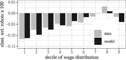
Elasticities of wage-distribution deciles with respect to a change in robots. Model moments are based on the calibrated model. Data moments are based on Figure 10, panel A, in Acemoglu and Restrepo (2020). For details, see Online Appendix C.4.

Open in new tab Download slide

The first four rows in Table 1 summarize how well the model captures the effect of a change in the price of robots on robot adoption as well and on participation. The price-elasticity of robot adoption in the model is close to its target. Turning to changes in participation, like in the data, losses in the model are concentrated among routine workers. However, robot adoption increases participation of manual and cognitive workers in the model but not in the data. Still, the qualitative relationship across occupations is preserved in the sense that participation “declines” most for routine workers, followed by cognitive workers and manual workers. The model also replicates the participation rate, employment, income shares, average annual labor income as well as moments related to the tax and transfer system, all summarized in the remainder of Table 1.

Table 1.

Open in new tab

Calibration—model vs. data.

Table C.4 in Online Appendix C summarizes the calibrated parameters for labor supply, the tax system, and the distributions of skills and participation costs. Table C.5 in Online Appendix C contains the calibrated production function parameters. The calibrated substitution elasticities between the three types of labor and robots are |$\kappa _{M}=3.27$|⁠, |$\kappa _{R}=2.84$|⁠, and |$\kappa _{C}=1.14$|⁠. Robots are thus slightly better substitutes for manual labor than for routine labor, while they are more complementary to cognitive labor. Even though these parameters suggest that cheaper robots should negatively affect manual workers’ wages, due to rich general-equilibrium interactions, it is routine workers whose wages fall as robots get cheaper.

5.2.4. Limitations

To match the impact of robots on wages and participation, I need a sufficiently flexible specification of the production function. While the specification in (39)–(41) provides this flexibility, it also introduces many parameters. Papers such as Krusell et al. (2000) use time-series data to estimate parameters of the production function. In contrast, I need to base my calibration on data for just two periods: before and after a change in robot adoption. As a result, the production-function parameters in my paper are less well identified than those based on a full time series of data. To give the reader a better sense of the calibration, Section C.5 in the Online Appendix contains a sensitivity analysis. I find that parameters |$\gamma _{B,R}$| and |$\kappa _{R}$| might be less precisely calibrated. To address this concern, I compute optimal robot taxes for a range of values for these parameters. I find that the optimal robot tax increases in both, |$\gamma _{B,R}$| and |$\kappa _{R}$|⁠, with |$\gamma _{B,R}$| having a stronger impact. Increasing |$\gamma _{B,R}$| lets the optimal robot tax turn from negative to positive at |$\gamma _{B,R}\approx 0.15$|⁠.

To further address concerns regarding robustness, I include in Section D in the Online Appendix computations based on the simple robot-tax formula. Using this formula, I do not need to assume a specification for the production function. I compute taxes for different wage responses to robot adoption. I find that the overall range of taxes is similar to the one generated by the calibrated model. The computations using the simple formula also address the point that wage responses to robot adoption may differ from those found by Acemoglu and Restrepo (2020), for example, when studying other countries or time periods.³³ Finally, a comment is in order regarding the time span underlying the calibration. Acemoglu and Restrepo (2020) study a period of about 15 years. Their results thus provide useful calibration targets for a medium-run analysis, but may be less informative for studying the long-run.

5.3. Simulation under the Status-Quo Tax System

To illustrate how the calibrated model works, I simulate a drop in the price of robots for an economy under the status-quo tax system (keeping |$\tau$|⁠, |$\lambda$|⁠, and b constant). To show the impact of raising the robot tax, I also simulate an economy in which the tax on robots is ten times higher than under the status-quo (⁠|$t_{B}=15.5\%$| instead of 1.55%). Outcomes are plotted in Figure 2.³⁴ I first discuss the effects of the robot-price drop.

Figure 2.

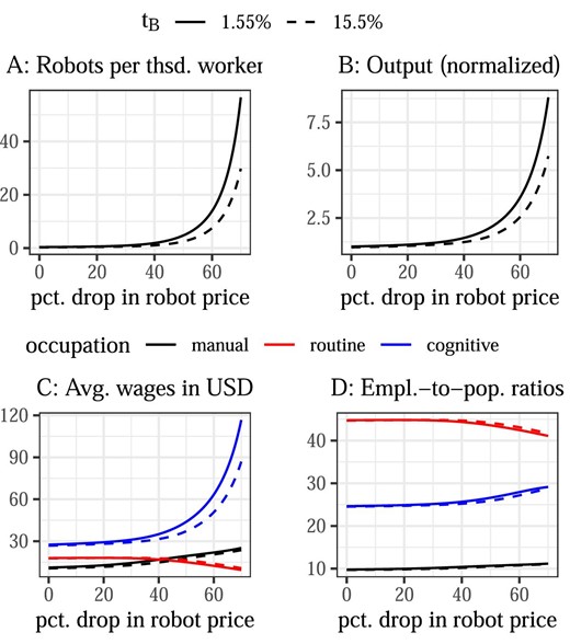
Effect of robot-price drop under status-quo and higher robot tax. The solid lines correspond to the status-quo tax system with a robot tax of 1.55%. The dashed lines correspond to a modified status-quo tax system with the only difference being a robot tax of 15.5%. Employment-to-population ratios represent the share of the population that participates in the labor market, categorized by occupation (not to be confused with the participation rate by occupation; summing the employment-to-population ratios gives the total participation rate).

Open in new tab Download slide

Lower robot prices lead to an increase in the number of robots per thousand workers (Panel A), which in turn leads to higher output (Panel B). As robots get cheaper, average wages of routine workers fall, while they rise for manual workers, and even more so for cognitive workers (Panel C).³⁵ At first, wage inequality between manual and routine workers thus decreases; however, once manual workers start to earn more than routine workers, wage inequality between these groups of workers goes up, and so does overall wage inequality. Changes in employment-to-population ratios are in line with wage changes: We see a drop in the share of participants who work in routine occupations, whereas the shares of participants who work in manual and cognitive occupations increases (Panel D).

Next, I turn to the effect of a higher robot tax, illustrated by the dashed lines in Figure 2. As the user price of robots is now higher, robot adoption goes down and so does output. At high robot prices, a tax on robots lowers average wages of manual and cognitive workers, while hardly affecting routine workers. In contrast, once robots get sufficiently cheap, routine workers’ wages benefit from the higher robot tax, while manual and cognitive workers lose. The effects on employment-to-population ratios are again in line with the effects on wages.

The experiment of increasing the robot tax illustrates the equity-efficiency tradeoff. The higher tax makes robots more expensive, thereby (further) distorting robot adoption and reducing efficiency. While the impact on robot adoption and output is unambiguously negative, the effect on wages and wage inequality is not. At high robot prices, as the larger robot tax leads wages of manual workers to fall relative to routine workers, inequality between manual and routine workers increases. At the same time, inequality between cognitive and routine workers decreases. Once robots are sufficiently cheap, a higher robot tax lowers overall inequality.

5.4. Optimal Taxes

Now, I compute the optimal tax system, which includes optimal taxes on the different types of capital, fully non-linear optimal taxes on labor income, as well as the optimal transfer to non-participants.³⁶

Optimal taxes on capital for different robot prices as well as optimal transfers to non-participants are shown in Figure 3. I first discuss Panel A: At high robot prices, it is optimal to subsidize robots at around |$t_{B}=-0.5\%$|⁠. When robots get cheaper, the robot subsidy turns into a tax. The tax reaches a maximum of around 1% once the price of robots has dropped by 50% and decreases thereafter. The optimal tax on equipment, |$t_{E}$|⁠, is positive throughout, starting at about |$1.5\%$|⁠, peaking at close to 2% once the robot price has dropped by about 55%, and decreasing thereafter. Finally, the optimal tax on structures is zero throughout.

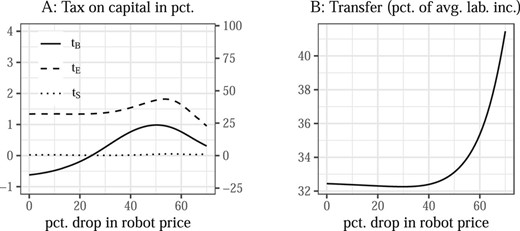
$Optimal capital taxes and transfer. In the left panel, $t_{B}$: tax on robots, $t_{E}$: tax on equipment, and $t_{S}$: tax on structures; left axis: tax on capital stocks (as in the model) and right axis: tax on capital income flows, assuming an annual return of 4.36% (see Section 5.2 for the reverse conversion from taxes on flows to taxes on stocks).$

Figure 3.

Optimal capital taxes and transfer. In the left panel, |$t_{B}$|⁠: tax on robots, |$t_{E}$|⁠: tax on equipment, and |$t_{S}$|⁠: tax on structures; left axis: tax on capital stocks (as in the model) and right axis: tax on capital income flows, assuming an annual return of 4.36% (see Section 5.2 for the reverse conversion from taxes on flows to taxes on stocks).

Open in new tab Download slide

To better understand the behavior of the optimal robot tax, I discuss in Online Appendix E the behavior of the different terms in the robot-tax formula. It turns out that robots are initially subsidized to compress inequality at the bottom of the wage distribution. As the price of robots drops, it becomes optimal to tax robots in order to reduce increasing wage inequality at the top. Eventually, the efficiency costs of taxing robots dominate equity gains and the optimal robot tax falls.

The optimal transfer to non-participants is first around 32% of average labor income and eventually increases to more than 40% (Panel B). The increase reflects that the economy gets richer overall as robots get cheaper, and it hence becomes feasible to pay more to non-participants.

Figure 4 shows optimal marginal and average income tax rates for different robot prices. Optimal marginal tax rates at the initial robot price exhibit the typical U-shape at lower incomes and then flatten off toward a maximum rate of around 63% (Panel A). At 50% and 70% lower robot prices, optimal marginal tax rates for low incomes increase, while they decrease for higher incomes. The higher marginal tax rates at lower incomes lead to more redistribution from high to low incomes.³⁷ This change is reflected in the optimal average tax rates shown in Panel B. At the initial robot price, average tax rates at lower incomes are regressive but become progressive towards higher incomes. The regressive nature at the bottom results from a positive tax bill for all participants. Once robots get cheaper, participants who earn low incomes receive a net transfer, making the tax system progressive overall. Moreover, at higher incomes, the progressivity of the tax system increases as the robot price falls, which is reflected in a larger slope of the average tax function. This higher progressivity corresponds to more relative redistribution from high to low incomes. The final observation is that average tax rates fall as robots get cheaper, reflecting that in richer economies the fixed revenue requirement can be met with lower average tax rates and that more revenue is raised with taxes on capital.

Figure 4.

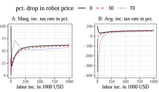
Optimal marginal and average income tax rates. The marginal income tax rate at the very top (not shown) is negative to exploit general-equilibrium effects for wage compression, as, for example, in Rothschild and Scheuer (2013). Average income tax rates at the initial robot price are locally regressive due to the exogenous revenue requirement. If this requirement were set to zero, average tax rates would be progressive also at the initial robot price.

Open in new tab Download slide

5.5. Welfare Impact of Different Tax Reforms

For governments to decide whether to reform their tax system, what ultimately matters is welfare. I therefore study the welfare impact of different tax reforms. I take as benchmark a CRP tax system in which income-tax progressivity and taxes on capital are fixed at their status-quo level, while I allow the revenue parameter |$\lambda$| and the transfer b to adjust in order to clear the budget constraint at different robot prices. I then compute the compensating variation of four reforms:

Reform 1: Set non-linear income taxes as well as the transfer optimally, while keeping taxes on capital at their status-quo level.
Reform 2: In addition to Reform 1, allow taxes on capital to be set optimally, under the restriction that taxes on robots and equipment must be equal.
Reform 3: On top of Reform 2, allow for different taxes on robots and equipment.
Reform 4: Starting from the status-quo, only set robot taxes optimally, while keeping taxes on other capital as well as income-tax progressivity unchanged.

To compute the compensating variation for the different reforms, I minimize the amount of additional resources that the government would need to achieve the same welfare under the benchmark tax system as under the reforms. The welfare gains of the three reforms can now be expressed as shares of GDP as well as in USD. I first compare reforms 1, 2, and 3 in Figure 5. Panel A shows the welfare gains of all three reforms compared to the benchmark. Panel B then zooms in on the differences between Reform 2 and Reform 1, and between Reform 3 and Reform 1.

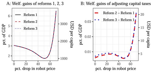
$Welfare effects of tax reforms. In Panel A, the lines represent the welfare-equivalent monetary value of the three tax reforms. Panel B shows the difference in these values between selected reforms, thereby capturing the gains from adjusting capital taxes. For example, $\text{Reform 2}-\text{Reform 1}$ captures the value of setting capital taxes optimally under the restriction that equipment and robots must be taxed at the same rate.$

Figure 5.

Welfare effects of tax reforms. In Panel A, the lines represent the welfare-equivalent monetary value of the three tax reforms. Panel B shows the difference in these values between selected reforms, thereby capturing the gains from adjusting capital taxes. For example, |$\text{Reform 2}-\text{Reform 1}$| captures the value of setting capital taxes optimally under the restriction that equipment and robots must be taxed at the same rate.

Open in new tab Download slide

Panel A shows that most welfare gains are achieved by Reform 1. Moving to a system with a fully non-linear optimal income tax delivers between 1.8% and 6.5% of GDP, which corresponds to between 1,000 and 4,000 USD per capita per year.³⁸ As robots get cheaper, the welfare gains of Reform 1 first fall, and then increase strongly after the price of robots has dropped by more than 60%. This pattern mirrors what happens to inequality in the economy. At first, cheaper robots reduce inequality, as manual workers gain, while routine workers lose (see also Figure 5.3); hence, redistribution becomes less necessary. Eventually, cognitive workers gain so much that inequality shoots up, the status-quo income tax becomes more and more suboptimal, and reforming it delivers large welfare gains.³⁹

Panel B shows that taxing structures and equipment differently, while taxing all equipment—including robots—at the same rate, delivers additional gains between 0.005 and 0.05% of GDP, or between 2 and 20 USD per capita per year (Reform 2 |$-$| Reform 1). Finally, allowing for different taxes on robots and equipment leads to welfare gains below 60 US cents per capita per year (the difference between the dotted blue line and the dashed red line).⁴⁰

Next, I turn to Reform 4. The results for optimal robot taxes and the welfare gains are shown in Figure 6. The robot tax is always higher than in the full optimum (compare Figure 3). The reason is that robot taxes are now used for redistribution that would otherwise have been achieved by the income tax. As robots get cheaper, the tax increases to more than 10%. Still, the welfare gains of this reform are much smaller than the gains from reforming the income tax system (compare Figure 5). Like for the other reforms, the gains increase strongly once the price of robots has dropped by more than 50%, reaching 0.5% of GDP, which corresponds to roughly 300 USD per capita per year. As cheaper robots lead to more inequality, the status-quo labor-income tax becomes increasingly suboptimal, for which adjusting the robot tax can partly compensate.^41,42

Figure 6.

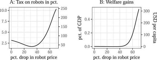
Optimal robot tax and welfare gains for Reform 4. Panel A, left axis: tax on capital stocks (as in the model); right axis: tax on capital income flows, assuming an annual return of 4.36% (see Section 5.2 for the reverse conversion from taxes on flows to taxes on stocks). In panel B, the line represents the welfare-equivalent monetary value of adjusting the robot tax.

Open in new tab Download slide

So far, I have focused on the overall welfare impact of reforming the tax system. Breaking down the welfare impact further, I find that non-participants gain, while for participants the results differ by occupation. When robots are still expensive, participants of all occupations lose compared to the status-quo. Once robots become cheaper, reforming robot taxation helps everyone, and the welfare decline for routine workers can be averted (see Online Appendix F for more details).

6. Conclusion

This paper studies the optimal taxation of robots, other capital, and labor income in a model with three occupations: manual, routine, and cognitive. I show theoretically that it is optimal to distort robot adoption to exploit general-equilibrium effects for wage compression. Wage compression alleviates income-tax distortions of labor supply, thereby raising welfare. Whether robots should be taxed or subsidized depends on their specific impact on wages. To build intuition, I first study a simple model with discrete types based on Stiglitz (1982). Since taxing robots increases wage inequality in some part of the wage distribution, while compressing wages in other parts, the sign of the optimal robot tax is ambiguous. Extending the simple model, the full model features continuous types and a participation margin, building on Rothschild and Scheuer (2013, 2014) and Jacquet, Lehmann, and Van der Linden (2013). I calibrate the full model to capture the effect of robots on the US labor market as estimated by Acemoglu and Restrepo (2020). In the optimal tax system, robots should initially be subsidized at about 0.5% to reduce inequality at the bottom of the wage distribution. As robots get cheaper and are adopted more widely, it becomes optimal to tax them at rates of up to 1% in order to compress wages at the top. However, as the efficiency costs of taxing robots become larger, the optimal robot tax eventually decreases. Equipment capital should be taxed at rates of up to 2%, whereas structures should go untaxed. Moreover, as robot adoption drives up income inequality, the optimal income tax should redistribute more from the rich to the poor. Finally, I study the welfare impact of reforming the status-quo tax system toward the optimum. Reforming the robot tax, while leaving the rest of the tax system unchanged, can lead to welfare gains in the order of a few hundred USD per capita per year—in particular, once large-scale robot adoption drives up income inequality. Routine workers gain most form such a reform. Still, the welfare gains from reforming labor income taxes are an order of magnitude larger. If taxes on labor income can be set optimally, taxing robots differently from other equipment capital delivers very small additional gains. Since categorizing equipment into robots and non-robots could prove difficult in practice, this is good news.

Notes

The editor in charge of this paper was Nicola Pavoni.

Acknowledgments

I am especially grateful to Florian Scheuer, Bas Jacobs, and Björn Brügemann for very helpful conversations and comments. I also thank Eric Bartelsman, Michael Best, Felix Bierbrauer, Nicholas Bloom, Raj Chetty, Iulian Ciobica, David Dorn, Aart Gerritsen, Renato Gomes, Emanuel Hansen, David Hemous, Jonathan Heathcote, Gee Hee Hong, Hugo Hopenhayn, Caroline Hoxby, Albert Jan Hummel, Guido Imbens, Pete Klenow, Wojciech Kopczuk, Tom Krebs, Dirk Krueger, Per Krusell, Simas Kucinskas, Sang Yoon Lee, Moritz Lenel, Jonas Löbbing, Davide Malacrino, Agnieszka Markiewicz, Magne Mogstad, Serdar Ozkan, Anil Rao, Pascual Restrepo, Juan Rios, Dominik Sachs, Michael Saunders, Ctirad Slavík, Isaac Sorkin, Kevin Spiritus, Nicolas Werquin, Frank Wolak, Hakkı Yazıcı, Ulrich Zierahn, Floris Zoutman, seminar participants at Erasmus University Rotterdam, VU Amsterdam, CPB Netherlands, the University of Mannheim, the Univsersity of Zurich, LMU Munich, the University of Cologne, and FU Berlin, and participants of the CESifo Public Economics Area Conference 2018, the EEA Congress 2018, the TASKS V Conference 2018, the Oslo-Penn-Toronto Conference on Macro Public Finance 2019, the NTA Conference 2019, and the IIPF Conference 2020 for valuable comments and suggestions. Finally, I thank co-editor Nicola Pavoni as well as four anonymous referees for many helpful comments. Financial support through ERC Grant No. 757721 is gratefully acknowledged. This paper has benefited from a research visit at Stanford University supported by the C. Willems Stichting.

Appendix: Optimal Robot Tax in the Simple Model

Assuming that only the adjacent downward-binding incentive constraints are relevant, maximized social welfare is given by the Lagrangian

$$\begin{eqnarray} \mathcal {L} &=& f_{M}\psi _{M}V_{M}+f_{R}\psi _{R}V_{R}+f_{C}\psi _{C}V_{C} \\ && +\, \mu \eta _{CR}\left(V_{C}-U\left(c_{R}\left(V_{R},\ell _{R}\right),\ell _{R}\frac{Y_{R}\left(\boldsymbol {L},K_{B}\right)}{Y_{C}\left(\boldsymbol {L},K_{B}\right)}\right)\right) \\ && +\, \mu \eta _{RM}\left(V_{R}-U\left(c_{M}\left(V_{M},\ell _{M}\right),\ell _{M}\frac{Y_{M}\left(\boldsymbol {L},K_{B}\right)}{Y_{R}\left(\boldsymbol {L},K_{B}\right)}\right)\right) \\ && +\, \mu \xi _{M}\left(f_{M}\ell _{M}-L_{M}\right)+\mu \xi _{R}\left(f_{R}\ell _{R}-L_{R}\right)+\mu \xi _{C}\left(f_{C}\ell _{C}-L_{C}\right) \\ && +\, \mu \left(\sum _{i}f_{i}\ell _{i}Y_{i}\left(\boldsymbol {L},K_{B}\right)+Y_{B}\left(\boldsymbol {L},K_{B}\right)K_{B}-\sum _{i}f_{i}c_{i}-q_{B}K_{B}\right), \end{eqnarray}$$

(A.1)

where μ is the multiplier on the resource constraint, |$\mu \eta _{CR}$| is the multiplier on the incentive constraint for cognitive workers, and |$\mu \eta _{RM}$| is the multiplier on the incentive constraint for routine workers. Moreover, |$\mu \xi _{i}$| is the multiplier on the labor-market-clearing condition for occupation i. To find an expression for the optimal robot tax, first write the resource constraint as |$Y\left(\boldsymbol {L},K_{B}\right)-\sum _{i}f_{i}c_{i}-q_{B}K_{B}=0$|⁠. Then, differentiate the Lagrangian with respect to |$K_{B}$| to obtain⁴³

$$\begin{eqnarray} \begin{aligned}\frac{\partial \mathcal {L}}{\partial K_{B}}= & -\mu \eta _{CR}U_{\ell }\left(c_{R}\left(V_{R},\ell _{R}\right),\ell _{R}\frac{Y_{R}}{Y_{C}}\right)\ell _{R}\frac{\partial }{\partial K_{B}}\left(\frac{Y_{R}}{Y_{C}}\right)\\ & -\mu \eta _{RM}U_{\ell }\left(c_{M}\left(V_{M},\ell _{M}\right),\ell _{M}\frac{Y_{M}}{Y_{R}}\right)\ell _{M}\frac{\partial }{\partial K_{B}}\left(\frac{Y_{M}}{Y_{R}}\right)\\ & +\mu \left(Y_{B}-q_{B}\right). \end{aligned} \end{eqnarray}$$

(A.2)

Define elasticities of relative wage rates with respect to robots as

$$\begin{eqnarray} \varepsilon _{Y_{C}/Y_{R},K_{B}}= & -\varepsilon _{Y_{R}/Y_{C},B}\equiv \frac{\partial }{\partial K_{B}}\left(\frac{Y_{R}}{Y_{C}}\right)\frac{Y_{C}}{Y_{R}}K_{B}, \end{eqnarray}$$

(A.3)

$$\begin{eqnarray} \varepsilon _{Y_{M}/Y_{R},K_{B}}\equiv & \frac{\partial }{\partial K_{B}}\left(\frac{Y_{M}}{Y_{R}}\right)\frac{Y_{R}}{Y_{M}}K_{B}. \end{eqnarray}$$

(A.4)

Use that

$$\begin{eqnarray} Y_{B}=p_{B}=\left(1+t_{B}\right)q_{B}\Leftrightarrow Y_{B}-q_{B}=t_{B}q_{B}, \end{eqnarray}$$

(A.5)

set (A.2) equal to zero, rearrange, and divide by μ to get

$$\begin{eqnarray} \begin{aligned}t_{B}q_{B}K_{B}= & -\eta _{CR}U_{\ell }\left(c_{R}\left(V_{R},\ell _{R}\right),\ell _{R}\frac{Y_{R}}{Y_{C}}\right)\ell _{R}\frac{Y_{R}}{Y_{C}}\varepsilon _{Y_{C}/Y_{R},K_{B}}\\ & +\eta _{RM}U_{\ell }\left(c_{M}\left(V_{M},\ell _{M}\right),\ell _{M}\frac{Y_{M}}{Y_{R}}\right)\ell _{M}\frac{Y_{M}}{Y_{R}}\varepsilon _{Y_{M}/Y_{R},K_{B}}. \end{aligned} \end{eqnarray}$$

(A.6)

Now define the incentive effects in a similar way to Rothschild and Scheuer (2013) (using that |$w_{i}=Y_{i}$| and suppressing some arguments):

$$\begin{eqnarray} I_{CR}\equiv -\eta _{CR}U_{\ell }\left(c_{R},\ell _{R}\frac{w_{R}}{w_{C}}\right)\ell _{R}\frac{w_{R}}{w_{C}}=\eta _{CR}\left(\ell _{R}\frac{w_{R}}{w_{C}}\right)^{1+\frac{1}{\varepsilon }} \end{eqnarray}$$

(A.7)

and

$$\begin{eqnarray} I_{RM}\equiv -\eta _{RM}U_{\ell }\left(c_{M},\ell _{M}\frac{w_{M}}{w_{R}}\right)\ell _{M}\frac{w_{M}}{w_{R}}=\eta _{RM}\left(\ell _{M}\frac{w_{M}}{w_{R}}\right)^{1+\frac{1}{\varepsilon }}, \end{eqnarray}$$

(A.8)

where I have used that with quasi-linear utility |$U_{\ell }=-\ell ^{\frac{1}{\varepsilon }}.$| Rewrite (A.6) as

$$\begin{eqnarray} t_{B}q_{B}K_{B}= \varepsilon _{Y_{C}/Y_{R},K_{B}}I_{CR}-\varepsilon _{Y_{M}/Y_{R},K_{B}}I_{RM}. \end{eqnarray}$$

(A.9)

Expressions for Incentive Effects.

To obtain expressions for the incentive effects (A.7) and (A.8), one needs to derive expressions for the multipliers |$\eta _{CR}$| and |$\eta _{RM}$|⁠. To do so, differentiate the Lagrangian in (A.1) with respect to indirect utilities to obtain

$$\begin{eqnarray} \frac{\partial \mathcal {L}}{\partial V_{M}}=f_{M}\psi _{M}-\mu \eta _{RM}U_{c}\left(c_{M},\ell _{M}\frac{w_{M}}{w_{R}}\right)\frac{\partial c_{M}}{\partial V_{M}}-\mu f_{M}\frac{\partial c_{M}}{\partial V_{M}}. \end{eqnarray}$$

(A.10)

Equating to zero, using that |$\partial c_{M}/\partial V_{M}=1/U_{c}\left(c_{M},\ell _{M}\right)$|⁠, and with quasi-linear utility |$U_{c}=1$| as well as |$\mu =1$|⁠, rearranging yields

$$\begin{eqnarray} \eta _{RM}=f_{M}\psi _{M}-f_{M}=f_{M}\left(\psi _{M}-1\right). \end{eqnarray}$$

(A.11)

Analogously, we obtain

$$\begin{eqnarray} \frac{\partial \mathcal {L}}{\partial V_{C}}=f_{C}\psi _{C}+\mu \eta _{CR}-\mu f_{C}\frac{\partial c_{C}}{\partial V_{C}}, \end{eqnarray}$$

(A.12)

which after equating to zero and using the properties of quasi-linear utility becomes

$$\begin{eqnarray} \eta _{CR}=f_{C}\left(1-\psi _{C}\right), \end{eqnarray}$$

(A.13)

such that the incentive effects are

$$\begin{eqnarray} I_{CR}=f_{C}\left(1-\psi _{C}\right)\left(\ell _{R}\frac{w_{R}}{w_{C}}\right)^{1+\frac{1}{\varepsilon }} \end{eqnarray}$$

(A.14)

and

$$\begin{eqnarray} I_{RM}=f_{M}\left(\psi _{M}-1\right)\left(\ell _{M}\frac{w_{M}}{w_{R}}\right)^{1+\frac{1}{\varepsilon }}. \end{eqnarray}$$

(A.15)

Footnotes

See, for example, this quote from a Draft report by the Committee on Legal Affairs of the European Parliament:

“Bearing in mind the effects that the development and deployment of robotics and AI might have on employment and, consequently, on the viability of the social security systems of the Member States, consideration should be given to the possible need to introduce corporate reporting requirements on the extent and proportion of the contribution of robotics and AI to the economic results of a company for the purpose of taxation and social security contributions;”

Bill Gates has advocated for a tax on robots. See https://qz.com/911968/bill-gates-the-robot-that-takes-your-job-should-pay-taxes/.

Figure 8, panel B, in their paper shows the impact of robots on employment by occupation. For none of the occupations is there a positive effect. In particular, employment in manual non-routine occupations stays flat. Even though the figure shows net impacts that may mask flows, there is no strong evidence of routine workers moving to manual non-routine jobs, which would be the most likely switch. The pronounced employment losses in routine occupations thus correspond to individuals exiting employment altogether.

Adao et al. (2020) find that adapting to technological transitions that are cognitively biased takes particularly long, as they rely on the young generations choosing new occupations, rather than on older generations switching occupations. Since this paper is also concerned with the medium run, and since automation is a cognitively biased technology, ruling out occupational mobility is a reasonable choice.

In Thuemmel (2018), I study an extension with occupational mobility (but without a participation margin) that generates similar magnitudes of optimal robot taxes and similar welfare effects of adjusting robot taxes as I find in this paper. Allowing for occupational mobility dampens the impact of robots. As a consequence, there is less need to intervene with robot taxes, which are therefore smaller in absolute value than in the case without occupational mobility. This result also hints at the long-run: In the long-run, it is likely that individuals would choose occupations that are less negatively affected by automation—which would diminish the case for robot taxation. At the extreme, if automation would not affect relative wages across occupations, robots should be neither taxed nor subsidized. Taxing or subsidizing robots is thus likely a medium-run rather than a long-run policy.

See also Koizumi (2020), who studies a model similar to Guerreiro, Rebelo, and Teles (2022) with an additional type of capital and the restriction that taxes on robots and other capital must be the same.

See also Oberson (2019), who focuses on the legal and practical aspects of taxing robots.

Saez (2004) refers to this as a violation of the labor-types-observability assumption.

Gomes, Lozachmeur, and Pavan (2018) set up a model in which workers with continuously distributed ability choose both, intensive margin labor supply and occupation, as they do in this paper. They then study optimal occupation-specific non-linear income taxation and show that occupational choice is optimally distorted. They refer to this as a distortion of production efficiency. In Scheuer (2014), occupational choice is distorted in the presence of occupation-specific taxes—however, production is efficient. Also see Scheuer and Werning (2016) for production efficiency despite general-equilibrium effects.

10.

Also related are papers that study the impact of robots on the economy theoretically (see Berg et al. 2018; Acemoglu and Restrepo 2018; Caselli and Manning 2019; Stähler 2021), as well as papers on labor-market polarization, for example, Acemoglu and Autor (2011), Autor and Dorn (2013), and vom Lehn (2020).

11.

See also Kina, Slavık, and Yazici (2019) and Slavík and Yazici (2019), who study a model like Slavík and Yazici (2014) but with incomplete markets. Slavík and Yazici (2019) focuses on the welfare implications of reforming the status-quo tax system by taxing structures and equipment at the same rate, whereas Kina, Slavık, and Yazici (2019) study optimal taxes on equipment and structures.

12.

Note that the assumption does not require the marginal products of non-routine labor to increase. All it requires is that these marginal products increase relatively more than the marginal product of routine labor. The assumption is thus also satisfied if all marginal products decrease, as long as the marginal product of routine labor decreases the most.

13.

I focus on a linear tax on robots since with a non-linear tax and constant returns to scale there would be incentives for firms to break up into parts until each part faces the same minimum tax burden. With linear taxes, such incentives are absent.

14.

In a direct mechanism, workers announce their type i, and then get assigned consumption |$c_{i}$| and labor supply |$\ell _{i}$|⁠. Here, I consider the equivalent problem in which instead of consumption, the planner allocates indirect utilities |$V_{i}$| and define |$c\left(V_{i},\ell _{i}\right)$| as the inverse of |$U\left(c_{i},\ell _{i}\right)$| with respect to its first argument.

15.

See also the discussion in Stiglitz (1982) regarding downward-binding incentive constraints.

16.

There are only three levels of wages, |$w_{M}$|⁠, |$w_{R}$|⁠, and |$w_{C}$|⁠. With inequality at the top of the distribution, I refer to the gap between |$w_{C}$| and |$w_{R}$|⁠. Inequality at the bottom of the distribution refers to the gap between |$w_{R}$| and |$w_{M}$|⁠.

17.

If one were to only distinguish between equipment and structures, robots would also be classified as equipment capital. In this paper, equipment capital thus refers to all equipment other than robots.

18.

Strictly speaking, |$f_{i}$| is not a density, since it does not integrate to 1. I refer to it as density nevertheless.

19.

The density of potential wages is the density of individuals who would earn wage w when participating in the labor market.

20.

I assume that the monotonicity condition is satisfied, that is, gross-income needs to increase in w. Together with the single-crossing condition, monotonicity ensures that the local incentive constraints are equivalent to the global incentive constraint (see e.g. Fudenberg and Tirole 1991, Theorems 7.2 and 7.3). I follow the common approach of dropping the monotonicity condition and verifying ex-post that it is satisfied.

21.

The optimal taxes on equipment capital and structures, |$t_{E}$| and |$t_{S}$|⁠, are characterized by expressions analogue to Proposition 2. See the derivations in Online Appendix B.

22.

In the simplified model, elasticities of relative wages coincide with elasticities of relative wage rates. Due to heterogeneity of wages within occupations, this is no longer the case here.

23.

In contrast, the utility of marginal participants has no impact on welfare, as they are indifferent as to whether to participate in the labor market.

24.

See Reed and Jorgensen (2004) for a discussion of the log-normal Pareto distribution. I use the single Pareto log-normal, which originates from equation (23) when |$\beta \rightarrow \infty$|⁠. Other papers that have used the Pareto log-normal include Rothschild and Scheuer (2016) and Lockwood, Nathanson, and Weyl (2017).

25.

Occupation-dependent participation–cost distributions would potentially allow me to better match participation responses later on. However, since participation costs are modeled as disutility of participation, in the optimal tax analysis, occupation-dependent distributions would lead to occupation-specific welfare weights. To see this, note that with occupation-dependence, two individuals with the same levels of consumption and labor supply could have different levels of utility if they worked in different occupations. Since I do not want optimal taxes to be driven by occupation-specific welfare weights, I choose a participation–cost distribution that is common to all individuals.

26.

Writing the production function in terms of |$K_{B}$| rather than in terms of |$K_{B,M}, K_{B,R}$|⁠, and |$K_{B,C}$| is possible due to the assumption that the firm optimally allocates robots to be used together with labor in the three occupations, such that the returns to robots are equalized, as specified below in (42). Moreover, I assume that the government cannot observe the allocation of robots inside the firm, and hence cannot tax |$K_{B,M}$|⁠, |$K_{B,R}$|⁠, and |$K_{B,C}$| at different rates.

27.

See also Figure G.2 in the Online Appendix for a graphical illustration of the nesting structure.

28.

See http://www.nber.org/data/morg.html.

29.

The data on industrial robots from the IFR (2014), which Acemoglu and Restrepo (2020) use start in 1993. For labor market outcomes, Acemoglu and Restrepo (2020) use Census Data for 1990 and 2000 and American Community Survey Data for 2007.

30.

Acemoglu and Autor (2011) use the labels “abstract” for cognitive non-routine and “services” for manual non-routine. See Cortes (2016) for the same classification and labels as used in this paper.

31.

The obtained level of R is kept constant across all simulations.

32.

All US dollar-values in the paper are in 2016-dollars.

33.

Chung and Lee (2021) use the same empirical framework as Acemoglu and Restrepo (2020) and find that the impact of robots on local employment in the US evolves over time and turns positive in more recent years. See also Graetz and Michaels (2018) for a panel of 17 countries, Dauth et al. (2019) for Germany, Acemoglu, Lelarge, and Restrepo (2020) for France, and Barth et al. (2020) for Norway.

34.

One may also think of the horizontal axis as time-axis. In the data, the price of robots has dropped by 60% over a span of 15 years (Graetz and Michaels 2018).

35.

The negative wage effects of robot adoption are concentrated among routine workers, who are (at least initially) mostly found in the lower-middle of the wage distribution. In contrast, the negative impact of robot adoption on the deciles of the wage distribution, as shown in Figure 1, is strongest at the bottom. This is because Figure 1 shows elasticities of deciles not changes in levels.

36.

The optimal tax system is computed using the optimal control software GPOPS-II (see Patterson and Rao 2014), which can be obtained from http://www.gpops2.com/.

37.

At the 70% price-drop, the marginal income-tax schedule exhibits a “double U-shape”, featuring one compressed “U” at the very bottom of the income distribution, followed by another, stretched-out “U” towards higher incomes. This is the result of the income density becoming bi-modal once incomes of cognitive workers shoot up and incomes of manual workers overtake those of routine workers.

38.

The dollar amounts are scaled based on per-capita GDP. Although the model is static, the welfare effects are therefore best thought of as per-year effects.

39.

These large gains are likely a lower bound, since I have calibrated the degree of inequality aversion such that it biases me against finding large benefits from reforming income taxation.

40.

See also Figure G.3 in the Online Appendix for welfare expressed as share of consumption.

41.

In Figure G.4 in the Online Appendix, I plot the outcomes of a tax reform, which optimally adjusts all taxes on capital, while income-tax progressivity is kept at the status-quo. Taxes on equipment are highest and increase most strongly as robots get cheaper. As the income tax becomes more and more suboptimal, taxes on capital are used for redistribution. A tax on equipment is most effective for redistributing from high to low incomes, since equipment capital is most complementary to cognitive labor.

42.

In the full optimum, robot taxes interact with the income tax schedule through general-equilibrium effects. In optimal tax models with endogenous wages (Stiglitz 1982; Rothschild and Scheuer 2013), general-equilibrium effects lead to optimal marginal tax rates on high incomes that are lower than those in a model with fixed wages, as this encourages labor supply, which in turn compresses the earnings distribution. Similarly, taxing robots has implications for individuals’ wages, labor supply, and earnings—and thus for optimal income taxes. By taxing robots, the government can achieve income compression and thus needs to distort labor supply less with income taxes to achieve the same amount of redistribution. As pointed out by Sachs, Tsyvinski, and Werquin (2020), in partial reforms of suboptimal tax schedules, such as those studied in this section, general-equilibrium effects operate in more intricate ways. In particular, raising the progressivity of the tax code in an already progressive tax system becomes more desirable than a model without general-equilibrium effects would suggest. For the general-equilibrium effects of capital taxation, see also Mayr (2021).

43.

In the derivations below, I omit arguments |$\boldsymbol {L},K_{B}$| in marginal products |$Y_{i}$| to help readability.

References

Acemoglu

Daron

Autor

David

(

2011

“Chapter 12—Skills, Tasks and Technologies: Implications for Employment and Earnings.”

Handbook of Labor Economics

, vol.

Part B

, edited by

Ashenfelter

Orley

Card

David

, pp.

1043

–

1171

Elsevier

Google Scholar

Google Preview

OpenURL Placeholder Text

WorldCat

Acemoglu

Daron

Lelarge

Claire

Restrepo

Pascual

(

2020

“Competing with Robots: Firm-Level Evidence from France.”

AEA Papers and Proceedings

110

383

–

388

Google Scholar

Crossref

WorldCat

Acemoglu

Daron

Manera

Andrea

Restrepo

Pascual

(

2020

“Does the US Tax Code Favor Automation?”

Brookings Papers on Economic Activity, 2020, 231–85

Acemoglu

Daron

Restrepo

Pascual

(

2018

“The Race between Man and Machine: Implications of Technology for Growth, Factor Shares, and Employment.”

American Economic Review

108

(

1488

–

1542

Google Scholar

Crossref

WorldCat

Acemoglu

Daron

Restrepo

Pascual

(

2020

“Robots and Jobs: Evidence from US Labor Markets.”

Journal of Political Economy

128

2188

–

2244

Google Scholar

Crossref

WorldCat

Adao

Rodrigo

Beraja

Martin

Pandalai-Nayar

Nitya

(

2020

“Technological Transitions with Skill Heterogeneity across Generations.”

NBER Working Paper No. 26625

NBER

Ales

Laurence

Kurnaz

Musab

Sleet

Christopher

(

2015

“Technical Change, Wage Inequality and Taxes.”

American Economic Review

105

(

3061

–

3101

Google Scholar

Crossref

WorldCat

Autor

David H.

Dorn

David

(

2013

“The Growth of Low-Skill Service Jobs and the Polarization of the US Labor Market.”

American Economic Review

103

(

1553

–

1597

Google Scholar

Crossref

WorldCat

Autor

David H.

Levy

Frank

Murnane

Richard J.

(

2003

“The Skill Content of Recent Technological Change: An Empirical Exploration.”

Quarterly Journal of Economics

118

1279

–

1333

Google Scholar

Crossref

WorldCat

Barro

Robert J.

Redlick

Charles J.

(

2011

“Macroeconomic Effects from Government Purchases and Taxes.”

Quarterly Journal of Economics

126

–

102

Google Scholar

Crossref

WorldCat

Barth

Erling

Roed

Marianne

Schone

Pal

Umblijs

Janis

(

2020

“How Robots Change Within-Firm Wage Inequality.”

IZA Discussion Paper 13605

Bénabou

Roland

(

2000

“Unequal Societies: Income Distribution and the Social Contract.”

American Economic Review

(

–

129

Google Scholar

Crossref

WorldCat

Bénabou

Roland

(

2002

“Tax and Education Policy in a Heterogeneous-Agent Economy: What Levels of Redistribution Maximize Growth and Efficiency?”

Econometrica

481

–

517

Google Scholar

Crossref

WorldCat

Berg

Andrew

Buffie

Edward F.

Zanna

Luis-Felipe

(

2018

“Should We Fear the Robot Revolution? (The Correct Answer Is Yes).”

Journal of Monetary Economics

117

–

148

Google Scholar

Crossref

WorldCat

Blundell

Richard

McCurdy

Thomas

(

1999

“Chapter 27 Labor Supply: A Review of Alternative Approaches.”

Handbook of Labor Economics

, vol.

Part A

, edited by

Ashenfelter

Orley C.

Card

David

, pp.

1559

–

1695

Elsevier

Google Scholar

Google Preview

OpenURL Placeholder Text

WorldCat

Brynjolfsson

Erik

McAfee

Andrew

(

2014

The Second Machine Age: Work, Progress, and Prosperity in a Time of Brilliant Technologies

. 1st ed.

W. W. Norton & Company

New York

Google Scholar

Google Preview

OpenURL Placeholder Text

WorldCat

Caselli

Francesco

Manning

Alan

(

2019

“Robot Arithmetic: New Technology and Wages.”

American Economic Review: Insights

(

–

Google Scholar

OpenURL Placeholder Text

WorldCat

Chung

Jong Hyun

Lee

Yong Suk

(

2021

“The Evolving Impact of Robots on Jobs.”

ILR Review

Cortes

Guido Matias

(

2016

“Where Have the Middle-Wage Workers Gone? A Study of Polarization Using Panel Data.”

Journal of Labor Economics

–

105

Google Scholar

Crossref

WorldCat

Cortes

Guido Matias

Jaimovich

Nir

Siu

Henry E.

(

2017

“Disappearing Routine Jobs: Who, How, and Why?”

Journal of Monetary Economics

–

Google Scholar

Crossref

WorldCat

Costinot

Arnaud

Werning

Iván

(

2022

“Robots, Trade, and Luddism: A Sufficient Statistic Approach to Optimal Technology Regulation.”

The Review of Economic Studies

(forthcoming)

Dauth

Wolfgang

Findeisen

Sebastian

Suedekum

Jens

Woessner

Nicole

(

2019

“The Adjustment of Labor Markets to Robots.”

Journal of the European Economic Association

3104

–

3153

Google Scholar

Crossref

WorldCat

Diamond

Peter A.

Mirrlees

James A.

(

1971

“Optimal Taxation and Public Production I: Production Efficiency.”

American Economic Review

(

–

Google Scholar

OpenURL Placeholder Text

WorldCat

Feldstein

Martin

(

1973

“On the Optimal Progressivity of the Income Tax.”

Journal of Public Economics

357

–

376

Google Scholar

Crossref

WorldCat

Ford

Martin

(

2015

Rise of the Robots: Technology and the Threat of a Jobless Future

Basic Books

New York

Google Scholar

Google Preview

OpenURL Placeholder Text

WorldCat

Frey

Carl Benedikt

Berger

Thor

Chen

Chinchih

(

2018

“Political Machinery: Did Robots Swing the 2016 US Presidential Election?”

Oxford Review of Economic Policy

418

–

442

Fudenberg

Drew

Tirole

Jean

(

1991

Game Theory

. 1st ed.

The MIT Press

Cambridge, MA

Google Scholar

Google Preview

OpenURL Placeholder Text

WorldCat

Gasteiger

Emanuel

Prettner

Klaus

(

2022

“Automation, Stagnation, and the Implications of a Robot Tax.”

Macroeconomic Dynamics

218

–

Google Scholar

Crossref

WorldCat

Gomes

Renato

Lozachmeur

Jean-Marie

Pavan

Alessandro

(

2018

“Differential Taxation and Occupational Choice.”

Review of Economic Studies

511

–

557

Google Scholar

Crossref

WorldCat

Graetz

Georg

Michaels

Guy

(

2018

“Robots at Work.”

Review of Economics and Statistics

100

753

–

768

Google Scholar

Crossref

WorldCat

Gravelle

Jane G.

(

2011

“Reducing Depreciation Allowances to Finance a Lower Corporate Tax Rate.”

National Tax Journal

1039

Google Scholar

Crossref

WorldCat

Guerreiro

Joao

Rebelo

Sergio

Teles

Pedro

(

2022

“Should Robots Be Taxed?”

The Review of Economic Studies

279

–

311

Google Scholar

Crossref

WorldCat

Heathcote

Jonathan

Storesletten

Kjetil

Violante

Giovanni L.

(

2017

“Optimal Tax Progressivity: An Analytical Framework.”

Quarterly Journal of Economics

132

–

Hémous

David

Olsen

Morten

(

2022

“The Rise of the Machines: Automation, Horizontal Innovation, and Income Inequality.”

American Economic Journal: Macroeconomics

179

–

223

Google Scholar

OpenURL Placeholder Text

WorldCat

IFR

(

2014

World Robotics: Industrial Robots

International Federation of Robotics

Google Scholar

Google Preview

OpenURL Placeholder Text

WorldCat

IFR

(

2020

International Federation of Robotics

https://my.worldrobotics.org/. Accessed October 17, 2020

Jacobs

Bas

(

2015

“Optimal Inefficient Production.”

Working paper

Erasmus University Rotterdam

Jacobs

Bas

Thuemmel

Uwe

(

2018

“Optimal Taxation of Income and Human Capital and Skill-Biased Technical Change.”

Working paper

Tinbergen Institute

OpenURL Placeholder Text

WorldCat

Jacobs

Bas

Thuemmel

Uwe

(

2022

“Optimal Linear Income Taxes and Education Subsidies under Skill-Biased Technical Change.”

International Tax and Public Finance

(forthcoming)

Google Scholar

OpenURL Placeholder Text

WorldCat

Jacquet

Laurence

Lehmann

Etienne

Van der Linden

Bruno

(

2013

“Optimal Redistributive Taxation with Both Extensive and Intensive Responses.”

Journal of Economic Theory

148

1770

–

1805

Google Scholar

Crossref

WorldCat

Kina

Ozlem

Slavık

Ctirad

Yazici

Hakki

(

2019

“Redistributive Capital Taxation Revisited.”

Working paper

European University Institute, CERGE-EI, Sabanci University

Koizumi

Hideto

(

2020

“Optimal Taxation of Intermediate Goods in a Partially Automated Society.”

Working paper

Hitotsubashi University

Krusell

Per

Ohanian

Lee E.

Ríos-Rull

José-Víctor

Violante

Giovanni L.

(

2000

“Capital-Skill Complementarity and Inequality: A Macroeconomic Analysis.”

Econometrica

1029

–

1053

Google Scholar

Crossref

WorldCat

Lockwood

Benjamin B.

Nathanson

Charles G.

Glen Weyl

(

2017

“Taxation and the Allocation of Talent.”

Journal of Political Economy

125

1635

–

1682

Google Scholar

Crossref

WorldCat

Loebbing

Jonas

(

2020

“Redistributive Income Taxation with Directed Technical Change.”

CESifo Working Paper 8743

Mayr

Lukas

(

2021

“Taxing Capital in the Presence of Trickle Down Effects: A Sufficient Statistics Approach.”

SSRN Scholarly Paper ID 3768717

Social Science Research Network, Rochester, NY

Meghir

Costas

Phillips

David

(

2010

“Labour Supply and Taxes.”

Dimensions of Tax Design: The Mirrlees Review

, edited by

Mirrlees

James A.

Adam

Stuart

Besley

Timothy

Blundell

Richard

Bond

Stephen

Chote

Robert

Gammie

Malcolm

Johnson

Paul

Myles

Gareth

Poterba

James

, pp.

202

–

274

Oxford University Press

Google Scholar

Google Preview

OpenURL Placeholder Text

WorldCat

Naito

Hisahiro

(

1999

“Re-Examination of Uniform Commodity Taxes under a Non-Linear Income Tax System and Its Implication for Production Efficiency.”

Journal of Public Economics

165

–

188

Google Scholar

Crossref

WorldCat

Naito

Hisahiro

(

2004

“Endogenous Human Capital Accumulation, Comparative Advantage and Direct vs. Indirect Redistribution.”

Journal of Public Economics

2685

–

2710

Google Scholar

Crossref

WorldCat

Oberson

Xavier

(

2019

Taxing Robots

Edward Elgar Publishing

Cheltenham

Patterson

Michael A.

Rao

Anil V.

(

2014

“GPOPS-II: A MATLAB Software for Solving Multiple-Phase Optimal Control Problems Using Hp-Adaptive Gaussian Quadrature Collocation Methods and Sparse Nonlinear Programming.”

ACM Transactions on Mathematical Software

1:1

–

1:37

Google Scholar

Crossref

WorldCat

Persson

Mats

(

1983

“The Distribution of Abilities and the Progressive Income Tax.”

Journal of Public Economics

–

Google Scholar

Crossref

WorldCat

Prettner

Klaus

Strulik

Holger

(

2020

“Innovation, Automation, and Inequality: Policy Challenges in the Race against the Machine.”

Journal of Monetary Economics

116

249

–

Google Scholar

Crossref

WorldCat

Reed

William J.

Jorgensen

Murray

(

2004

“The Double Pareto-Lognormal Distribution—A New Parametric Model for Size Distributions.”

Communications in Statistics —Theory and Methods

1733

–

1753

Google Scholar

Crossref

WorldCat

Rothschild

Casey

Scheuer

Florian

(

2013

“Redistributive Taxation in the Roy Model.”

Quarterly Journal of Economics

128

623

–

668

Google Scholar

Crossref

WorldCat

Rothschild

Casey

Scheuer

Florian

(

2014

“A Theory of Income Taxation under Multidimensional Skill Heterogeneity.”

Working paper

Wellesley College, Stanford University

Rothschild

Casey

Scheuer

Florian

(

2016

“Optimal Taxation with Rent-Seeking.”

Review of Economic Studies

1225

–

1262

Google Scholar

Crossref

WorldCat

Sachs

Dominik

Tsyvinski

Aleh

Werquin

Nicolas

(

2020

“Nonlinear Tax Incidence and Optimal Taxation in General Equilibrium.”

Econometrica

469

–

493

Google Scholar

Crossref

WorldCat

Saez

Emmanuel

(

2002

“Optimal Income Transfer Programs: Intensive versus Extensive Labor Supply Responses.”

Quarterly Journal of Economics

117

1039

–

1073

Google Scholar

Crossref

WorldCat

Saez

Emmanuel

(

2004

“Direct or Indirect Tax Instruments for Redistribution: Short-Run versus Long-Run.”

Journal of Public Economics

503

–

518

Google Scholar

Crossref

WorldCat

Scheuer

Florian

(

2014

“Entrepreneurial Taxation with Endogenous Entry.”

American Economic Journal: Economic Policy

126

–

Google Scholar

OpenURL Placeholder Text

WorldCat

Scheuer

Florian

Werning

Iván

(

2016

“Mirrlees Meets Diamond-Mirrlees.”

NBER Working Paper No. 22076

NBER

Schulz

Karl

Tsyvinski

Aleh

Werquin

Nicolas

(

2022

“Generalized Compensation Principle.”

FRB WP 2022-18

Federal Reserve Bank of Chicago

OpenURL Placeholder Text

WorldCat

Shourideh

Hosseini

(

2018

“Inequality, Redistribution, and Optimal Trade Policy: A Public Finance Approach.”

Working paper

Carnegie Mellon University

Slavík

Ctirad

Yazici

Hakki

(

2014

“Machines, Buildings, and Optimal Dynamic Taxes.”

Journal of Monetary Economics

–

Google Scholar

Crossref

WorldCat

Slavík

Ctirad

Yazici

Hakki

(

2019

“On the Consequences of Eliminating Capital Tax Differentials.”

Canadian Journal of Economics

225

–

252

Google Scholar

Crossref

WorldCat

Stähler

Nikolai

(

2021

“The Impact of Aging and Automation on the Macroeconomy and Inequality.”

Journal of Macroeconomics, 67

Stiglitz

Joseph E.

(

1982

“Self-Selection and Pareto Efficient Taxation.”

Journal of Public Economics

213

–

240

Google Scholar

Crossref

WorldCat

Thuemmel

Uwe

(

2018

“Optimal Taxation of Robots.”

CESifo Working Paper 7317. vom Lehn, Christian (2020).

vom Lehn

Christian

(

2020

“Labor Market Polarization, the Decline of Routine Work, and Technological Change: A Quantitative Analysis.”

Journal of Monetary Economics

110

–

Google Scholar

Crossref

WorldCat

Zhang

Pengqing

(

2019

“Automation, Wage Inequality and Implications of a Robot Tax.”

International Review of Economics & Finance

500

–

509

Google Scholar

Crossref

WorldCat

This is an Open Access article distributed under the terms of the Creative Commons Attribution License (https://creativecommons.org/licenses/by/4.0/), which permits unrestricted reuse, distribution, and reproduction in any medium, provided the original work is properly cited.

Download all slides

Month:	Total Views:
November 2022	41
December 2022	12
January 2023	379
February 2023	163
March 2023	145
April 2023	248
May 2023	240
June 2023	420
July 2023	624
August 2023	314
September 2023	261
October 2023	248
November 2023	262
December 2023	220
January 2024	263
February 2024	331
March 2024	291
April 2024	179
May 2024	196
June 2024	145
July 2024	107
August 2024	108
September 2024	128
October 2024	153
November 2024	174
December 2024	139
January 2025	105
February 2025	121
March 2025	126
April 2025	134
May 2025	34

Article Contents

Optimal Taxation of Robots

Abstract

1. Introduction

2. Related Literature

3. Simple Model to Build Intuition

3.1. Setup

3.1.1. Workers, Occupations and Preferences

3.1.2. Technology

3.1.3. Government and Tax Instruments

3.2. Optimal Policy

3.2.1. Optimal Robot Tax

4. Full Model

4.1. Setup

4.1.1. Skill Heterogeneity

4.1.2. Preferences and Participation

4.1.3. Technology

4.2. Optimal Taxation

4.2.1. Optimal Robot Tax

4.2.2. Marginal Income Taxes

5. Quantitative Analysis

5.1. Functional Forms

5.2. Calibration

5.2.1. Data and Calibration Targets

5.2.2. Calibration Procedure

5.2.3. Calibration Outcomes

5.2.4. Limitations

5.3. Simulation under the Status-Quo Tax System

5.4. Optimal Taxes

5.5. Welfare Impact of Different Tax Reforms

6. Conclusion

Notes

Acknowledgments

Appendix: Optimal Robot Tax in the Simple Model

Expressions for Incentive Effects.

Footnotes

References

Supplementary data

Citations

Views

Altmetric

Email alerts

Citing articles via

Latest

Most Read

Most Cited

This Feature Is Available To Subscribers Only