


Abstract
Received wisdom suggests that most exporters sell most of their output domestically. We show, however, that the distribution of export intensity varies substantially across countries and is often bimodal, displaying “twin peaks”—that is, large shares of both low- and high-intensity exporters coexisting alongside each other within a country. We reconcile this new stylized fact with an otherwise standard model of trade in which firms face firm-destination-specific revenue shifters that follow a lognormal distribution with sufficiently high dispersion. We structurally estimate the model and show that differences in countries’ size relative to the rest of the world can account for most of the observed cross-country variation in the distribution of export intensity in our data. While policies that incentivize firms to export a high share of their output account for a substantial share of the variation in the dispersion of firm-destination revenue shifters, they cannot fully account for the widespread prevalence of twin peaks around the world.
A set of Teaching Slides to accompany this article are available online as Supplementary Data.
1. Introduction
Received wisdom suggests that the majority of exporters in a country sell most of their output domestically, while only a very small minority of them concentrate their sales abroad (Bernard et al. 2003; Brooks 2006; Arkolakis 2010; Eaton, Kortum, and Kramarz 2011). In this paper, we show that this perception—based primarily on data from large and developed economies—fails to characterize the distribution of export intensity, the share of a firm’s revenues accounted for by exports (conditional on exporting) in small or developing countries.
Our first contribution is to show that export intensity distributions vary tremendously across countries and—crucially—that rather than being an oddity, distributions featuring twin peaks are quite common across the world. This is vividly illustrated in Figure 1. Countries like Argentina, Russia, and South Africa, shown in the uppermost panel of the figure, exhibit the same pattern identified in previous studies: Firms with an export intensity below 0.2 constitute more than half of exporters, while firms with an export intensity above 0.8 account for less than 10% of exporters. In Lao PDR, Pakistan, and Vietnam, we observe the opposite pattern—the share of exporters with an intensity below 0.2 and above 0.8 is, on average, 16% and 54%, respectively. A large number of countries—as many as 47 out of the 72 in our data—and as diverse as China, Namibia, and Romania, instead exhibit “twin peaks”, that is, a high concentration of firms on both ends of the export intensity distribution.
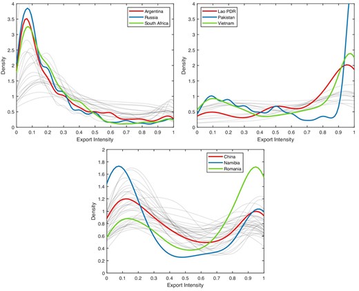
Export Intensity Distribution across countries and selected examples. The figure depicts the kernel density of export intensity, or the share of total sales accounted for by exports among exporters, for each country in our data (in light gray lines) with selected examples (in bold colored lines). The data comes from several waves of the World Bank Enterprise Survey and are described in detail in Section 3. Countries are partitioned in three groups based on the value of the Hartigan and Hartigan (1985) dip test of unimodality presented in Figure 5 below. The countries included in each panel of the figure are listed in Appendix D.
In previous work, Lu (2010) and Defever and Riaño (2017a) documented the marked bimodality of the distribution of export intensity in China. We now show that twin peaks in the distribution of export intensity are not a phenomenon specific to China. In so doing, we contribute to the literature pioneered by Bernard and Jensen (1995), Roberts and Tybout (1996), and Bernard and Jensen (1999) that uncovered the key stylized facts characterizing the behavior of exporters and spurred the heterogeneous firm revolution in international trade.1
Using harmonized firm-level data for 72 (mostly developing and transition) countries drawn from the World Bank Enterprise Surveys (WBESs), we show that bimodality remains a salient feature of the distribution of export intensity regardless of how we slice our data. Since we observe a significant share of low-intensity exporters in most countries, twin peaks arise where large numbers of high-intensity exporters operate as well. We find that these are more likely to be foreign-owned, engaged in assembly and processing activities; they are also more prevalent in certain sectors (e.g. textiles and clothing), in less developed countries; and where subsidies subject to export share requirements (ESRs) are available. While these results are consistent with the existing empirical evidence available (see e.g. Díaz de Astarloa et al. 2013; Antràs and Yeaple 2014; Dai, Maitra, and Yu 2016; Manova and Yu 2016; Defever and Riaño 2017a), they do not fully account for the high prevalence of twin peaks we observe across the world. As a case in point, even when we exclude firms that export all their output, we find that one-third of the countries in our data still have bimodal export intensity distributions. Export intensity distributions are also bimodal within industries, at the bilateral level (in the limited number of cases for which we observe firms’ exports to specific destinations), and when we consider datasets other than WBESs.
Our second contribution is to show that a simple model with isoelastic demand à la Melitz (2003) can naturally generate twin peaks and account for the observed variation in the distribution of export intensity across countries quite successfully. The key assumption we require is heterogeneity at the firm-destination-level, rather than just at the firm level, as it is the case in most workhorse models of trade with heterogeneous firms.2 A large body of empirical work has shown that firm-destination-specific factors account for a substantial share of the variation of firm-level exports (e.g. Kee and Krishna 2008; Crozet, Head, and Mayer 2012; Lawless and Whelan 2014; Munch and Nguyen 2014; Bas, Mayer, and Thoenig 2017). Heterogeneity at the firm-destination-level can be due to multiple causes such as cross-country differences in tastes (Crozet, Head, and Mayer 2012), differences in the quality necessary to sell products in a given market (Brooks 2006; Verhoogen 2008), firms’ participation in global value chains (Antràs and de Gortari 2020) or distortions such as privileged access to export markets (Khandelwal, Schott, and Wei 2014), fiscal incentives offered in special economic zones (SEZs) only to high-intensity exporters (Defever and Riaño 2017a; Defever et al. 2019), and export subsidies granted to firms selling only in specific foreign markets (Defever et al. 2020), just to mention a few.
Treating the firm-destination-specific revenue shifters that generate this heterogeneity in our model as random variables following lognormal distributions, we derive a closed-form expression for the probability density function (pdf) of export intensity. We show that this distribution is bimodal when the sum of the variances of domestic and export revenue shifters is sufficiently high. The modes are located near 0 and 1, and their “height” is determined by a country’s relative market size with respect to the rest of the world: that is, in relatively large countries, most exporters operate with a low export intensity, while in small countries, the majority of exporters tend to be high-intensity ones; in countries of intermediate size, the distribution of export intensity exhibits twin peaks instead—just as Figure 1 shows.3
We estimate the structural parameters that govern the distribution of export intensity of each country—the sum of the variances of revenue shifters (the shape parameter) and relative market size (the scale parameter)—using the WBES data. To do so, we first show that there is a one-to-one relationship that is independent of the shape parameter between a country’s median export intensity and its relative market size vis-à-vis the rest of the world. This allows us to tease out the latter directly from the data without having to solve for the full general equilibrium of the model.4 Conditional on relative market size, we then estimate the shape parameter by maximum likelihood. The identification of this parameter is very transparent: If the conditions for twin peaks are satisfied, then greater dispersion of revenue shifters increases the distribution’s mass in the boundaries of the support. Conversely, if dispersion is low, then the distribution of export intensity is unimodal, and its mass is tightly concentrated around the median in the interior of the support.
The estimates of the shape and scale parameters reveal that the conditions for bimodality are satisfied for all countries in our data. How can we reconcile this result with the fact that statistical tests indicate that one-third of the countries in our data have unimodal distributions? To investigate this, we pool all our data across countries and estimate a single-shape-parameter model in which firms from all countries draw their domestic and export revenue shifters from distributions with the same shape parameter. Doing so implies that all cross-country variation in the distribution of export intensity is due to differences in relative size. The results we obtain are remarkable. Our model not only accounts for most of the variation in the distribution of export intensity we observe across the world, but can also explain the “discrepancy” we outlined above—relatively small and large countries have distributions that “look” unimodal—in the sense that a statistical test does not reject unimodality—while countries of intermediate size display prominent twin peaks.
We leverage the single-shape-parameter model and estimate it across several subsets of observations (various types of exporters, industries, and countries) with two objectives: to determine whether the conditions for bimodality are met for each subsample, and to gauge the contribution of each group to the magnitude of the overall dispersion of revenue shifters. Our results reveal that observable characteristics that are associated with higher firm-level export intensity, such as foreign ownership, participation in export processing, and having been an exporter for a long time, among others, account—individually—for between 7% and 25% of the overall variance of revenue shifters, depending on the specification. Excluding firms that export all their output altogether reduces the variance of revenue shifters by 42%. Crucially, however, even under these stringent conditions, the level of dispersion we estimate is still sufficiently high to generate twin peaks. Thus, our results show that policies that incentivize firms to export a high share of their output, which have been shown to have the potential to be highly distortive by Defever and Riaño (2017a) and Brooks and Wang (2016), account for a substantial share of the dispersion of revenue shifters. Nevertheless, these cannot fully account for the ubiquity of export intensity distributions characterized by twin peaks that we observe across the world.
Ours is not the first paper to incorporate sources of heterogeneity in addition to productivity to a model of international trade with heterogeneous firms. Among these, our paper is most closely related to state-of-the-art quantitative models of exports at the firm-level, such as Eaton, Kortum, and Kramarz (2011) and Fernandes et al. (2018), which also feature lognomal-distributed firm-destination-specific revenue shifters. We differ from Eaton, Kortum, and Kramarz (2011) and Fernandes et al. (2018) in two key respects, however: the dimensions of the data we aim to explain and the use we give to our quantitative model. While Eaton, Kortum, and Kramarz (2011) seek to reproduce the variation in French firms’ sales across markets and Fernandes et al. (2018) focus on the intensive margin of exports, we are interested instead in explaining the differences in the distribution of export intensity across countries. In a similar vein, we utilize our model to investigate what are the observable characteristics that account for the high dispersion in firms’ sales across markets and that in turn generate twin peaks, while Eaton, Kortum, and Kramarz and Fernandes et al. focus on quantifying the effect of a reduction in trade costs on welfare. Our finding that a high dispersion of exporters’ sales across markets allows us to explain why export intensity distributions differ so much around the world is similar in spirit to the results of Armenter and Koren (2015). They show that the Melitz (2003) model requires a substantial amount of size-independent heterogeneity to reproduce simultaneously the share of exporters and their size premium observed in US data.
The rest of the paper is organized as follows. Section 2 discusses why it is important to understand the export intensity distribution and model it accurately. Section 3 presents the data used in the paper, documents the prevalence of twin peaks in the distribution of export intensity across countries and different subsamples, reports statistical tests of unimodality and contrasts the distributions generated by the WBES data to those obtained from more representative datasets. Section 4 presents our theoretical framework. In it, we derive a closed-form expression for the pdf of export intensity and characterize the conditions under which the distribution of export intensity is bimodal. Section 5 presents our identification strategy and the estimates from our structural model. With our estimates at hand, we explore the relationship between twin peaks and relative market size and gauge the contribution of different factors to the prevalence of bimodality across countries. Section 6 concludes.
2. Why is the Export Intensity Distribution Important?
Export intensity measures the relative importance of foreign sales for a firm. For this reason, the mean export intensity has been used extensively in models of trade with heterogeneous firms to pin down the magnitude of costs that impede international flows of goods. Notable examples include Melitz and Redding (2015) and Head, Mayer, and Thoenig (2014) in models with two symmetric countries, Eaton, Kortum, and Kramarz (2011) in a multi-country environment and Atkeson and Burstein (2010) and Alessandria and Choi (2014) in dynamic models.
A common feature of these models is that the variable cost associated with exporting is the same for all firms selling to a given destination. Several policies that distort the relative incentives to export vis-à-vis selling domestically are firm-specific, however. Some prominent examples include the allocation of export quota rights (Khandelwal, Schott, and Wei 2014) and the provision of subsidies targeted at specific subsets of firms, for example, according to their location or foreign ownership status (Farole and Akinci 2011), whether they export the majority of their output or sell it in specific markets (Defever and Riaño 2017a; Defever et al. 2019, 2020), or if they produce goods considered to be of “‘strategic importance” (Westphal 1990; Kalouptsidi 2018). The common theme across these different policies is that they distort the incentives to export relative to selling domestically differently across firms.
In order to quantify the impact of these policies on aggregate outcomes such as productivity and welfare, it is therefore necessary to infer what the distribution of export intensity would have been in the absence of distortions. The idea is analogous to the approach pioneered by Guner, Ventura, and Yi (2008), Restuccia and Rogerson (2008), and Hsieh and Klenow (2009) to measure the consequences of the mis-allocation of resources across firms. Defever and Riaño (2017a) provide one example of this approach. They study how a tax deduction granted to firms exporting more than 70% of their output affects aggregate welfare in China. They show that this policy distorts the export intensity distribution by inducing a subset of firms to export a larger share of their output than they would otherwise do. The welfare cost is increasing in the difference between the observed distribution of export intensity and the counterfactual distribution that would have arisen had the policy not been in place. The welfare cost of a given subsidy is larger in a country that is relatively large with respect to the rest of the world like China—where the majority of exporters would have naturally operated at a low export intensity—than in a smaller country like Sri Lanka or Vietnam, where export requirement would not be binding for most firms and making subsidies subject to these less distortive. Defever and Riaño construct the undistorted counterfactual distribution by combining the export intensity distributions of large developing countries that do not provide subsidies subject to ESRs. Alternatively, Brooks and Wang (2016) use a two-country Melitz (2003) model, which predicts a degenerate export intensity distribution as their starting point, and interpret any differences across firms as wedges in the efficient allocation of sales across markets. In this context, they then show that the variance of the ratio of export to domestic sales is a sufficient statistic for welfare when wedges follow a lognormal distribution.
Recent research has shown that firms’ response to external shocks—most notably to real exchange rate (RER) depreciations—is substantially heterogeneous across the distribution of export intensity. Alfaro et al. (2017) find that while firms in East Asia increase their productivity, experience faster growth in sales and invest more in R&D following an RER depreciation, firms in Latin America respond in the diametrically opposite way, and firms in industrialized countries do not exhibit any significant change. They show that this heterogeneous response is due to the fact that firms in Latin America are substantially less export-intensive than firms in East Asia—a pattern that we also observe in our data and that our model can readily reproduce (see Figure 8 below). RER depreciations increase firms’ demand the most when firms have a high export intensity, and in so doing, also help to relax financial constraints, allowing firms to overcome the fixed costs involved in R&D investment. Closely related, Kohn, Leibovici, and Szkup (2020) show that the response of aggregate exports to large RER depreciations is fundamentally shaped by the distribution of export intensity when firms rely on foreign currency borrowing to finance their investment. Under these circumstances, a large RER depreciation increases a firm’s demand for exports, while simultaneously raising its borrowing costs and tightening financial constraints. In an economy in which the majority of exporters have low export intensity, firms can expand their exports much faster in response to a depreciation because they can reallocate their sales from the domestic to the export market without having to expand their capital stock. This margin of adjustment, on the other hand, is dampened in countries where high-intensity exporters are more prevalent.
The shape of the export intensity distribution also affects the sales diversification benefits that firms achieve from exporting. When firms are buffeted by idiosyncratic demand shocks across markets, selling both domestically and abroad reduces the volatility of the growth rate of their sales (Riaño 2011; Vannoorenberghe 2012). In Defever and Riaño (2017b), we show that there is a U-shaped relationship between the volatility of a firm’s sales growth and its export intensity. This implies that when a country’s export intensity distribution exhibits twin peaks, the volatility-dampening benefits of exporting are significantly reduced because most exporters have intensities either near 0 or 1.
3. Data and Stylized Fact
3.1. Data Description
Our data comes from several waves of the WBESs spanning the period 2002–2016. These surveys are carried out by the World Bank’s Enterprise Analysis Unit using a uniform methodology and core questionnaire and are designed to be representative of a country’s non-agricultural private economy.5 The unit of observation is the establishment, that is, a physical location where business is carried out or industrial operations take place, which should have its own management and control over its own workforce. Since the vast majority of establishments surveyed report to be single-establishment firms, hereafter we refer to them as “firms”. We use data for the manufacturing sector only—that is, firms that belong to ISIC Rev. 3.1 sectors 15–37.
The WBES provides information on firms’ main sector of operation, age, total sales, export intensity, ownership status (whether the firm is domestic or foreign-owned), labor productivity, and the share of material inputs accounted for by imports. Some survey waves provide information on the first year a firm began exporting, the number of products it produces (at the 4-digit ISIC industry level) and bilateral export sales to specific destinations. Export intensity—our key variable of interest—is defined as the share of sales that a firm exports directly or indirectly through an intermediary in a fiscal year and therefore takes values in the interval (0,1].6
Table 1 provides information on the number of exporters and the number of WBES survey waves per country. Our sample consists of 72 developing and transition countries (with the exception of Ireland and Sweden), for which we observe at least 97 exporting firms when we pool the data across all available survey waves.7 In terms of geographic coverage, the countries in our data are evenly distributed across Eastern Europe, Latin America and the Caribbean, Asia, and the Middle East and Africa; Ireland and Sweden are the only two countries from Western Europe. Table 1 also indicates whether a country provides subsidies subject to ESRs—incentives directly conditioned on firms’ export intensity. Examples of these incentives, which are most frequently used in SEZs and duty-drawback regimes, include cash transfers, tax holidays and deductions, and the provision of utilities at below-market rates (Defever and Riaño 2017a; Defever et al. 2019).8 Table 1 shows that half the countries in our data offer this class of subsidies.
Sample composition.
| Country | Code | Survey waves | # Exporters | ESR | Country | Code | Survey waves | # Exporters | ESR | |
|---|---|---|---|---|---|---|---|---|---|---|
| Albania | ALB | 2002, 05, 07, 13 | 116 | No | Lithuania | LTU | 2002, 04, 05, 09, 13 | 258 | No | |
| Argentina | ARG | 2006, 10 | 1,140 | No | Madagascar | MDG | 2005, 09, 13 | 256 | Yes | |
| Armenia | ARM | 2002, 05, 09, 13 | 170 | No | Malaysia | MYS | 2002, 15 | 735 | Yes | |
| Bangladesh | BGD | 2002, 07, 13 | 1,255 | Yes | Mauritius | MUS | 2005, 09 | 183 | No | |
| Belarus | BLR | 2002, 05, 08, 13 | 146 | Yes | Mexico | MEX | 2006, 10 | 727 | No | |
| Bolivia | BOL | 2006, 10 | 242 | No | Moldova | MDA | 2002, 03, 05, 09, 13 | 221 | No | |
| Bosnia-Herzegovina | BIH | 2002, 05, 09, 13 | 200 | Yes | Morocco | MAR | 2004, 13 | 585 | Yes | |
| Brazil | BRA | 2003, 09 | 832 | Yes | Namibia | NAM | 2006, 14 | 109 | Yes | |
| Bulgaria | BGR | 2002, 04, 05, 07, 09, 13 | 538 | No | Nicaragua | NIC | 2003, 06, 10 | 283 | Yes | |
| Chile | CHL | 2004, 06, 10 | 1,001 | No | Nigeria | NGA | 2007, 14 | 316 | Yes | |
| China | CHN | 2002, 03, 12 | 1,439 | Yes | Pakistan | PAK | 2002, 07, 13 | 534 | Yes | |
| Colombia | COL | 2006, 10 | 703 | No | Panama | PAN | 2006, 10 | 134 | No | |
| Costa Rica | CRI | 2005, 10 | 238 | Yes | Paraguay | PRY | 2006, 10 | 246 | Yes | |
| Croatia | HRV | 2002, 05, 07, 13 | 335 | No | Peru | PER | 2006, 10 | 701 | Yes | |
| Czech Republic | CZE | 2002, 05, 09, 13 | 232 | No | Philippines | PHL | 2003, 09, 15 | 914 | Yes | |
| Ecuador | ECU | 2003, 06, 10 | 385 | No | Poland | POL | 2002, 03, 05, 09, 13 | 439 | No | |
| Egypt | EGY | 2004, 13 | 676 | Yes | Romania | ROU | 2002, 05, 09, 13 | 290 | No | |
| El Salvador | SLV | 2003, 06, 10, 16 | 840 | No | Russian Fed. | RUS | 2002, 05, 09, 12 | 468 | No | |
| Estonia | EST | 2002, 05, 09, 13 | 175 | No | Senegal | SEN | 2003, 07, 14 | 148 | Yes | |
| Ethiophia | ETH | 2002, 11, 15 | 118 | Yes | Serbia | SRB | 2002, 03, 05, 09, 13 | 330 | No | |
| FYR Macedonia | MKD | 2002, 05, 09, 13 | 191 | No | Slovak Republic | SVK | 2002, 05, 09, 13 | 164 | No | |
| Ghana | GHA | 2007, 13 | 159 | Yes | Slovenia | SVN | 2002, 05, 09, 13 | 245 | No | |
| Guatemala | GTM | 2003, 06, 10 | 580 | Yes | South Africa | ZAF | 2003, 07 | 558 | No | |
| Honduras | HND | 2003, 06, 10 | 345 | Yes | Sri Lanka | LKA | 2004, 11 | 403 | Yes | |
| Hungary | HUN | 2002, 05, 09, 13 | 300 | No | Sweden | SWE | 2014 | 286 | No | |
| India | IND | 2002, 06, 14 | 2,212 | Yes | Syrian Arab Republic | SYR | 2003 | 251 | No | |
| Indonesia | IDN | 2003, 09, 15 | 720 | Yes | Tanzania | TZA | 2003, 06, 13 | 222 | Yes | |
| Ireland | IRL | 2005 | 97 | No | Thailand | THA | 2004, 16 | 1,066 | Yes | |
| Jordan | JOR | 2006, 13 | 377 | No | Tunisia | TUN | 2013 | 213 | Yes | |
| Kazakhstan | KAZ | 2002, 05, 09, 13 | 116 | No | Turkey | TUR | 2002, 04, 05, 08, 13 | 2,152 | Yes | |
| Kenya | KEN | 2003, 07, 13 | 511 | No | Uganda | UGA | 2003, 06, 13 | 221 | Yes | |
| Korea, Republic | KOR | 2005 | 99 | No | Ukraine | UKR | 2002, 05, 08, 13 | 435 | No | |
| Kyrgyz Republic | KGZ | 2002, 03, 05, 09, 13 | 126 | No | Uruguay | URY | 2006, 10 | 467 | No | |
| Lao PDR | LAO | 2006, 12, 16 | 128 | No | Uzbekistan | UZB | 2002, 03, 05, 08, 13 | 112 | Yes | |
| Latvia | LVA | 2002, 05, 09, 13 | 161 | No | Vietnam | VNM | 2005, 09, 15 | 1,251 | Yes | |
| Lebanon | LBN | 2006, 13 | 252 | No | Zambia | ZMB | 2002, 07, 13 | 146 | Yes |
Table 2 provides a first pass at the WBES data comparing exporters, across the distribution of export intensity, with domestic firms. Columns (1)–(3) provide information on firm size and productivity relative to the average value of the respective statistic in each country-survey year pair, while columns (4) and (5) report the percentage of foreign-owned firms and the use of imported inputs in each cell, respectively. Table 2 reveals that—consistent with the evidence summarized by Bernard et al. (2007) and Melitz and Redding (2014)—exporters are larger (both in terms of employment and output) and more productive than domestic firms. Looking across the export intensity distribution, we find that although there is a positive correlation between firm size and export intensity, there is not a clear relationship between labor productivity and export intensity.9 Columns (4) and (5) show that exporters—and high-intensity ones in particular—are more likely to be foreign-owned and to use imported intermediate inputs more intensively than domestic firms, consistent with the evidence documented by Antràs and Yeaple (2014) and Amiti and Konings (2007).
Firm characteristics by export status and export intensity.
| Employment | Output | Output per worker | % foreign-owned | % imported inputs | |
|---|---|---|---|---|---|
| (1) | (2) | (3) | (4) | (5) | |
| Non-exporters | 0.5 | 0.5 | 0.8 | 6.0 | 23.7 |
| Exporters | |||||
| Export intensity: | |||||
| |$\; \; \in (0.0,0.2]$| | 1.7 | 2.1 | 1.4 | 17.4 | 37.7 |
| |$\; \; \in (0.2,0.4]$| | 1.5 | 1.8 | 1.3 | 18.8 | 35.6 |
| |$\; \; \in (0.4,0.6]$| | 1.7 | 1.9 | 1.3 | 21.0 | 35.2 |
| |$\; \; \in (0.6,0.8]$| | 2.3 | 2.3 | 1.4 | 23.0 | 35.4 |
| |$\; \; \in (0.8,1.0]$| | 2.2 | 2.3 | 1.6 | 31.1 | 41.0 |
Notes. Columns (1)–(3) report the average across countries of the relative size and labor productivity of exporters and domestic firms relative to the mean value of each variable calculated in each country-survey year cell. Thus, for instance, domestic firms across all countries in our sample are 50% smaller (in terms of employment) than the average firm, while exporters with an export intensity lower than 20% are 70% larger than the average firm. Column (4) reports the percentage of foreign-owned firms (firms with a share of foreign equity at least 10% or greater), and column (5) presents the percentage of imported inputs in total intermediate inputs in each export intensity bin.
3.2. The Distribution of Export Intensity Across Countries
Figure 2 provides a bird’s eye view of the export intensity distribution across all countries in our data. In it we calculate the share of exporters across five export intensity bins in each country and present the distribution of these shares in each bin. Figure 2 shows that in the majority of countries, exporters concentrate in the first and last export intensity bins—that is, they either sell most of their output domestically or abroad—while the shares of exporters in the middle bins are substantially lower. The figure also shows that there is a high degree of heterogeneity across countries in terms of the share of high- and low-intensity exporters.
![Cross-country distribution of the share of exporters operating in different export intensity bins—all exporters. For each country in our data, we calculate the share of exporters operating across five export intensity bins ((0,0.2], (0.2,0.4], (0.4,0.6], (0.6,0.8], and (0.8,1]). The figure presents the main quantiles of the distribution of these shares across countries for each export intensity bin. The median is denoted by a circle; the top and bottom sides of each box denote, respectively, the 25th and 75th percentiles; the bottom and top of the “whiskers” (represented with dashed lines) indicate the minimum and maximum, respectively.](https://oup.silverchair-cdn.com/oup/backfile/Content_public/Journal/jeea/20/3/10.1093_jeea_jvac006/2/m_jvac006fig2.jpeg?Expires=1749047555&Signature=CpOtQGfeA7Co7XPTb~Pk4qTuHbsd7SsTp4HdhbqJtNFJlgDTTBCmGTtvF5iXByAp8n5nDODn8~3lkZg-clmqyukPj3QmQTmJbWWEPtCI4xreBB7yJ~p4o~NxmaJiCwuWzIXBWNazZ8vbP0~PDLLDAYZ5KufMoqII8WMm9qjgwP0N35N04HRW-g~HUc5qpRmRSESGGYdfmZ9ntTljBLjMSVfOs~QT6UxUpiqln9pOh5ZOCYHJkpMURFYzqkZttLL~cMI75Eb03RZVtp2YXBAvhTxOV1ermuxA9c6WvkMJjjmtzj4a~-5SP8gZQCK0zzUDGh0Q4yHn0ImuoeZJbm-j9w__&Key-Pair-Id=APKAIE5G5CRDK6RD3PGA)
Cross-country distribution of the share of exporters operating in different export intensity bins—all exporters. For each country in our data, we calculate the share of exporters operating across five export intensity bins ((0,0.2], (0.2,0.4], (0.4,0.6], (0.6,0.8], and (0.8,1]). The figure presents the main quantiles of the distribution of these shares across countries for each export intensity bin. The median is denoted by a circle; the top and bottom sides of each box denote, respectively, the 25th and 75th percentiles; the bottom and top of the “whiskers” (represented with dashed lines) indicate the minimum and maximum, respectively.
One plausible explanation for the existence of twin peaks in the export intensity distribution is that the distribution at the country level is a mixture of “standard” low-intensity exporters and a significant number of firms that export most of their output. We take advantage of the rich information available in WBESs to ascertain whether the twin peaks of the export intensity distribution are due to a composition effect driven by specific types of high-intensity exporters.
There are several factors that could potentially account for the prevalence of high-intensity exporters. For instance, Antràs and Yeaple (2014) document that foreign-owned affiliates are more export oriented than locally-owned firms in their respective host countries, while Ruhl and Willis (2017) find that exporters increase their export intensity gradually over time. Firms specialized in processing and assembly activities tend to exhibit high export intensities because they are required to export all goods that incorporate duty-free inputs (Dai, Maitra, and Yu 2016; Manova and Yu 2016). Lower wages in poorer countries also induce local exporters to specialize in more upstream stages of production, leading them to ship all their output downstream along global value chains, as Antràs and de Gortari (2020) show. Yet another possibility is a composition effect of the export intensity distributions of different industries, be it due to technology differences or comparative advantage (Brooks 2006; Bernard et al. 2007).
WBES identifies firms as being foreign-owned if the share of foreign equity is at least 10%. We classify firms as “processing exporters” if imports account for 90% or more of their expenditure on intermediate inputs, since WBES does not directly identify firms that rely on a processing customs regime to export. We denote “pure exporters” as those firms that export all their output. This group encompasses firms engaged in assembly activities or that belong to a global value chain (regardless of whether they are foreign-owned or not) as well as firms producing goods with no domestic demand, such as woolen sweaters sown in Bangladesh (Díaz de Astarloa et al. 2013). Single-product exporters are defined at the 4-digit ISIC industry level10 and “old” exporters are those with 10 years or more of exporting experience.11 The data on exports to specific destinations is available for a few countries, and the respective destinations considered vary according to the country of origin.12
Trade policy can also induce firms to export a high share of their output. Over the last three decades, developing countries have relied intensively on industrial policies aimed at fostering exports—most notably, the provision of generous fiscal incentives to firms located in SEZs (Rodrik 2004). Similarly, firms located in countries offering subsidies subject to ESRs—which as we have noted above, account for half of the countries in our sample—are only eligible to receive these if their export intensity exceeds a specified threshold (Defever and Riaño 2017a; Defever et al. 2019). Since developing countries tend to rely more intensively on distortive commercial policies than developed countries, as Goldberg and Pavcnik (2016) document, it is also plausible that twin peaks tend to arise mostly among the former. We are therefore interested in determining whether the shape of export intensity distributions is systematically related to a country’s level of development.
Figure 3 presents the share of exporters operating in each export intensity bin for the different subsets of exporters defined above and Figure 4 does the same across manufacturing sectors. The key message delivered by Figure 2 still holds regardless of how we slice the data: Most exporters operate at either a very low or very high export intensity—that is, they either sell less of 20% of their sales abroad, or they export more than 80% of them. Bimodality is a salient feature of the export intensity distribution—even within industries and for bilateral exports.13
![Cross-country distribution of the share of exporters operating in different export intensity bins across subsamples. For each country with more than 50 exporters in our data, we calculate the share of exporters operating across five export intensity bins ((0,0.2], (0.2,0.4], (0.4,0.6], (0.6,0.8], and (0.8,1]). The figure presents the main quantiles of the distribution of these shares across countries for each export intensity bin. The median is denoted by a circle, the top and bottom sides of each box denote, respectively, the 25th and 75th percentiles; the bottom and top of the “whiskers” (represented with dashed lines) indicate the minimum and maximum, respectively. The first panel in the first row excludes firms that are foreign-owned; the second excludes processing exporters and the third excludes firms with export intensity exactly equal to 1 (pure exporters). In the second row, the first panel excludes single-product exporters; the second excludes “old” exporters (firms that have exported for more than 10 years) and the third excludes observations from countries that offer subsidies subject to ESRs. In the third row, we present the distributions for OECD and non-OECD countries in the first two panels, respectively; the last panel presents the distribution based on the subsample of firms for which we observe their bilateral export intensity to selected destinations—that is, the share of total sales of firms in the origin country accounted for by exports sold only in the destination country.](https://oup.silverchair-cdn.com/oup/backfile/Content_public/Journal/jeea/20/3/10.1093_jeea_jvac006/2/m_jvac006fig3.jpeg?Expires=1749047555&Signature=46W4MOH9zuzuLUglHZftEkalVsPgSpHyj~qV9f2EvMmYhlbpuUPIXAwjD~cRM4c3OP~36GG9PvCrCNZjfsxO090PD-Xm75tYBlmcqw8jtYf5YVGp2aYpVgRoEqFbD9eXHOOKDfLESxs7wTuZ9mvttHX7XQz~5pyGaA53sSMIaU26o4W94Ni2jaiSihRTLsAXPCaxDhn4DnC-GHQN-qRrT6ANRGp~Phmnia~QQlnbH6l4prBwaugOSC6tHwFnC6O76OazjL18FcKcA7LUKsAdY~RAx83wifpnHPKdUsBMknEHdNXYRJj2tZ~tNk60MCDbl7nN80X7F3RrkhF~bvdoow__&Key-Pair-Id=APKAIE5G5CRDK6RD3PGA)
Cross-country distribution of the share of exporters operating in different export intensity bins across subsamples. For each country with more than 50 exporters in our data, we calculate the share of exporters operating across five export intensity bins ((0,0.2], (0.2,0.4], (0.4,0.6], (0.6,0.8], and (0.8,1]). The figure presents the main quantiles of the distribution of these shares across countries for each export intensity bin. The median is denoted by a circle, the top and bottom sides of each box denote, respectively, the 25th and 75th percentiles; the bottom and top of the “whiskers” (represented with dashed lines) indicate the minimum and maximum, respectively. The first panel in the first row excludes firms that are foreign-owned; the second excludes processing exporters and the third excludes firms with export intensity exactly equal to 1 (pure exporters). In the second row, the first panel excludes single-product exporters; the second excludes “old” exporters (firms that have exported for more than 10 years) and the third excludes observations from countries that offer subsidies subject to ESRs. In the third row, we present the distributions for OECD and non-OECD countries in the first two panels, respectively; the last panel presents the distribution based on the subsample of firms for which we observe their bilateral export intensity to selected destinations—that is, the share of total sales of firms in the origin country accounted for by exports sold only in the destination country.
![Cross-country distribution of the share of exporters operating in different export intensity bins across manufacturing sectors. For each country-sector pair with more than 50 exporters in our data, we calculate the share of exporters operating across five export intensity bins ((0,0.2], (0.2,0.4], (0.4,0.6], (0.6,0.8], and (0.8,1]). The figure presents the main quantiles of the distribution of these shares across countries for each export intensity bin for each manufacturing sector. The median is denoted by a circle, the top and bottom sides of each box denote, respectively, the 25th and 75th percentiles; the bottom and top of the “whiskers” (represented with dashed lines) indicate the minimum and maximum, respectively.](https://oup.silverchair-cdn.com/oup/backfile/Content_public/Journal/jeea/20/3/10.1093_jeea_jvac006/2/m_jvac006fig4.jpeg?Expires=1749047555&Signature=cEFA66ReSXBHzUiw2BtyS~uOCSqFc~MnKhCIYDY47Lbjvl33UpyaFwt6iBva9YlPK-XHXB~C22YCtLKjQJH5-GcVT64Z-XUgQQr1HmhpiWCtQrF-6zNOH0reLqgyxqbO7zvcNbDzHOl96oIYXHmjSEueb8m69MiFrMHWmqLJZ2Xn~KWrnoZX27ejwyPsPH2uCok1jFxqyaVRZKZrauo0-ZRLj2WT0hCR2VsYwDZE8SkXxbNmC2wBuFGP3AhYXonG84yrEGexy4xa~skGOYmazyR72E2gzuein~AWjiK5pX6HyOXUlodyDkzVwsxwLShIB5F4mGCOQ4VVLQXoaWWZKw__&Key-Pair-Id=APKAIE5G5CRDK6RD3PGA)
Cross-country distribution of the share of exporters operating in different export intensity bins across manufacturing sectors. For each country-sector pair with more than 50 exporters in our data, we calculate the share of exporters operating across five export intensity bins ((0,0.2], (0.2,0.4], (0.4,0.6], (0.6,0.8], and (0.8,1]). The figure presents the main quantiles of the distribution of these shares across countries for each export intensity bin for each manufacturing sector. The median is denoted by a circle, the top and bottom sides of each box denote, respectively, the 25th and 75th percentiles; the bottom and top of the “whiskers” (represented with dashed lines) indicate the minimum and maximum, respectively.
3.3. Test of Unimodality
We now shift our focus to the distribution of export intensity within countries; more specifically, we seek to identify which countries have bimodal export intensity distributions and which ones do not. We use the dip test statistic proposed by Hartigan and Hartigan (1985) to do so.14 The dip statistic measures departures from unimodality in the empirical cumulative distribution function (cdf), by relying on the fact that a unimodal distribution has a unique inflection point.15 As Henderson, Parmeter, and Russell (2008) note, the dip measures the amount of “stretching” needed to render the empirical cdf of a multi-modal distribution unimodal; therefore, a higher value of the dip leads to a rejection of the null hypothesis of unimodality.16
It is important to note that the dip test only allows us to infer whether the null hypothesis of unimodality is rejected or not, while kernel density based tests, such as Silverman (1981), can identify the number of modes in the data. There are two reasons why we prefer the dip test over the Silverman (1981) one to classify countries. First, unlike the dip test, density-based tests are highly sensitive to the choice of the bandwidth parameter. Second, the Silverman test is not well suited for data that, while continuous in nature like our export intensity data, exhibits clustering at figures that are multiples of 5%.17 The dip test, on the other hand, can be adjusted to take into account the discreteness of the data. Despite the advantages of the dip statistic, calculating the Silverman test reveals that the number of modes never exceeds two in any country in our data. Therefore, we classify a country as having a unimodal export intensity distribution if its dip test statistic is not rejected at the 1% significance level; otherwise, we consider it to be bimodal.
Figure 5 presents the dip statistic for each country in our sample. We find that the distribution of export intensity is bimodal in 47 out of 72 countries. This result stands in sharp contrast with the existing literature suggesting that this distribution is generally unimodal, with a majority of exporters selling a small share of their output abroad.
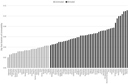
Dip test of unimodality of export intensity. The figure reports the value of the Hartigan and Hartigan (1985) dip test statistic of unimodality. Countries are identified as having a unimodal export intensity distribution if their dip statistic does not reject the null hypothesis of unimodality at the 1% confidence level; otherwise, they are identified as bimodal. The reported value of the dip statistic is calculated as the mean across 1,000 bootstrapped samples of 200 exporters drawn for each country. The algorithm used to calculate the dip test statistic is adjusted to take into account the discreteness of the export intensity data.
We next calculate the dip test across the different subsamples presented in Figure 3. Excluding foreign-owned and processing exporters has little effect on the number of countries we classify as bimodal, although countries such as Costa Rica, Croatia, and Hungary—notable for their success in attracting multinational firms—are reclassified as being unimodal. While we observe bimodality in the distributions of OECD and non-OECD countries, we find that this feature is more prevalent among countries that incentivize high-intensity exporters. Excluding firms that export all their output from the data altogether makes a significant dent in the prevalence of bimodality, increasing the number of countries with unimodal distributions from 25 to 46. Thus, our results show that the existence of twin peaks is not fully accounted for by the prevalence of a specific type of exporter operating within countries. Lastly, we calculate the dip statistic for country-sector pairs with more than 50 exporters and find that among the countries that we identify as bimodal based on their aggregate export intensity distribution, more than half of the distributions within sectors are themselves bimodal.
3.4. Comparing WBES with More Representative Surveys
An important concern is that twin peaks could be an artefact of the WBES data. Asker, Collard-Wexler, and Loecker (2014), for instance, note that the stratification procedure across sectors, size categories, and geographic locations used in the construction of the WBES leads to oversampling of larger firms. Although it is not clear why this would necessarily increase the likelihood of observing bimodal export intensity distributions, we show that twin peaks in the distribution of export intensity also arise in more representative datasets.
To this end, we asked fellow researchers to calculate for us the share of exporters across export intensity bins using well-known firm-level manufacturing surveys for a subsample of 13 countries in our data, which we then compared with the same moments calculated from WBES.18 The countries that we consider include five that we classify as unimodal (Argentina, Chile, Colombia, Indonesia, and South Africa) and eight that are bimodal (China, Hungary, India, Ireland, Pakistan, Thailand, Uruguay, and Vietnam). Most surveys we used for this analysis include all manufacturing firms with more than 10–20 employees, although the data for China and Ireland are based on surveys of larger firms. It is also important to note that the distribution of export intensity based on manufacturing surveys is calculated with data for a single year, whereas our main data set pools exporters from all survey waves available for a given country in the WBES.
Table 3 presents the results of our comparison and shows that the WBES provides an accurate picture of the distribution export intensity. Both the WBES and the different alternative data sources yield similar results with regard to the existence or not of twin peaks—even in the cases in which there are sizeable differences in the share of exporters in individual bins (such as Hungary and India). Crucially, in all countries but one, the share of exporters with export intensity in the middle bins is higher in the WBES than in the more representative data. Thus, the results presented in Figure 5 seem to, if anything, underestimate how common bimodal export intensity distributions are across the world.
Comparison of export intensity distributions—WBESs versus other surveys.
| # | Share of exporters with export intensity |$\in$|: | ||||||
|---|---|---|---|---|---|---|---|
| Country | Survey | Exporters | (0.0,0.2] | (0.2,0.4] | (0.4,0.6] | (0.6,0.8] | (0.8,1.0] |
| Argentina | ENIT | 830 | 0.660 | 0.123 | 0.071 | 0.065 | 0.081 |
| WBES | 1,140 | 0.535 | 0.225 | 0.102 | 0.067 | 0.071 | |
| Chile | ENIA | 900 | 0.582 | 0.116 | 0.113 | 0.093 | 0.096 |
| WBES | 1,001 | 0.490 | 0.186 | 0.098 | 0.065 | 0.162 | |
| China | NBS | 50,902 | 0.221 | 0.101 | 0.091 | 0.101 | 0.486 |
| WBES | 1,439 | 0.282 | 0.198 | 0.116 | 0.093 | 0.311 | |
| Colombia | EAM | 1,332 | 0.643 | 0.157 | 0.068 | 0.038 | 0.095 |
| WBES | 703 | 0.459 | 0.273 | 0.128 | 0.067 | 0.073 | |
| Hungary | APEH | 7,143 | 0.488 | 0.127 | 0.081 | 0.079 | 0.225 |
| WBES | 300 | 0.243 | 0.207 | 0.160 | 0.123 | 0.267 | |
| India | Prowess | 3,133 | 0.576 | 0.136 | 0.088 | 0.071 | 0.129 |
| WBES | 2,212 | 0.260 | 0.214 | 0.116 | 0.072 | 0.338 | |
| Indonesia | Census | 3,949 | 0.124 | 0.097 | 0.089 | 0.127 | 0.563 |
| WBES | 720 | 0.125 | 0.172 | 0.144 | 0.139 | 0.419 | |
| Ireland | FAME | 151 | 0.371 | 0.093 | 0.079 | 0.099 | 0.358 |
| WBES | 97 | 0.330 | 0.155 | 0.113 | 0.082 | 0.320 | |
| Pakistan | FRBP | 6,043 | 0.207 | 0.056 | 0.041 | 0.043 | 0.652 |
| WBES | 534 | 0.148 | 0.146 | 0.109 | 0.062 | 0.536 | |
| South Africa | SARS-NT | 7,530 | 0.844 | 0.076 | 0.036 | 0.025 | 0.019 |
| WBES | 558 | 0.529 | 0.279 | 0.113 | 0.020 | 0.060 | |
| Thailand | OIE | 1,591 | 0.302 | 0.136 | 0.111 | 0.121 | 0.331 |
| WBES | 1,066 | 0.147 | 0.151 | 0.134 | 0.141 | 0.427 | |
| Uruguay | EAAE | 389 | 0.424 | 0.131 | 0.090 | 0.095 | 0.260 |
| WBES | 467 | 0.328 | 0.173 | 0.105 | 0.103 | 0.291 | |
| Vietnam | ASE | 4,946 | 0.292 | 0.108 | 0.094 | 0.115 | 0.391 |
| WBES | 1,251 | 0.173 | 0.128 | 0.065 | 0.104 | 0.530 | |
Notes. Argentina: National Survey on Innovation and Technological Behavior of Industrial Argentinean Firms (ENIT) for the year 2001; this is a representative sample of establishments with more than ten employees. Chile: Annual National Industrial Survey (ENIA) for the year 2000, covering the universe of Chilean manufacturing plants with ten or more workers. Colombia: Annual Manufacturing Survey (EIA) for the year 1991, covering the universe of Colombian manufacturing plants with 10 or more workers. China: National Bureau of Statistics (NBS) Manufacturing Survey for the year 2003, which includes state-owned enterprises and private firms with sales above 5 million Chinese Yuan. Hungary: the universe of manufacturing firms for the year 2014 drawn from APEH, the Hungarian tax authority. India: Prowess database collected by the Centre for Monitoring the Indian Economy (CMIE) for the year 2001. Indonesia: Indonesian Census of Manufacturing Firms for the year 2009, which surveys all registered manufacturing plants with more than 20 employees. Ireland: FAME database collected by Bureau van Dijk for the year 2007. Pakistan: export intensity is constructed from two administrative datasets from the Federal Board of Revenue of Pakistan (FBRP); export figures are from customs records and domestic sales from VAT data records. The data records all firms with an annual turnover above 2.5 million Pakistani rupees for the year 2013. South Africa: South African Revenue Service and National Treasury Firm-Level Panel (SARS-NT) for the year 2010, which covers the universe of all tax-registered firms. Thailand: Annual Survey of Thailand’s Manufacturing Industries by the Office of Industrial Economics (OIE) for the year 2014. The questionnaire’s response rate is about 60% of all firms, accounting for about 95% of total manufacturing. Uruguay: Annual Survey of Economic Activity (EAAE), which covers all manufacturing plants with ten or more employees for the year 2005. Vietnam: Annual Survey on Enterprises (ASE) for the year 2010, which covers all state-owned enterprises, foreign-owned firms, and domestic private firms with more than ten employees.
4. Theoretical Framework
4.1. Model
We assume that the revenue shifters |$z_i\!(\omega )$| are random variables following a lognormal distribution with mean 0, variance |$\sigma ^2_{ zi}$| and pdf |$f(z_i)$| for |$i\in \lbrace d,x\rbrace$|. The lognormal distribution has gained increased prominence in the international trade literature (see e.g. Head, Mayer, and Thoenig 2014; Nigai 2017; Hanson, Lind, and Muendler 2018; Mrázová, Neary, and Parenti 2021). Recent work has shown that it not only fits better the complete distribution of sales—rather than just the right tail as the Pareto distribution—but also delivers more realistic implications for the trade elasticity and the welfare gains from trade (Bas, Mayer, and Thoenig 2017; Fernandes et al. 2018).
The lognormal distribution has two key properties that we take advantage of for our purposes: (i) it is closed under scalar multiplication, which means that the scaled revenue shifters, |$Z_d\!(\omega )\equiv s_dz_d\!(\omega )$| and |$Z_x\!(\omega )\equiv s_xz_x\!(\omega )$| defined in (2), are also lognormal; and (ii) the ratio of two lognormal random variables is also lognormal. Since |$E$| can be expressed as a strictly increasing function of the ratio of export to domestic revenue shifters, |$Z\equiv Z_x/Z_d$|, the latter property allows us to apply the method of transformations for random variables to derive a closed-form expression for the pdf of export intensity. This yields our first result.
See Appendix A.1.
As equation (3) shows, the distribution of export intensity is characterized by two parameters, the relative size of the domestic market compared to the foreign one, |$s_d/s_x$| (which we will also refer to as the scale parameter), and the sum of the variances of domestic and export revenue shifters, |$\sigma ^2_{ zd}+\sigma ^2_{ zx}$| (the shape parameter). Figure A.1 in Appendix A.1 provides examples of the pdf of export intensity for different values of the shape and scale parameters. The distribution (3) is known in statistics as the logit-normal distribution;20 its key properties have been derived by Johnson (1949).
We now move to describe the conditions under which the distribution of export intensity is bimodal. These are spelled out in our second proposition.
See Appendix A.2.
Proposition 2 says that when the sum of the variances of revenue shifters is sufficiently high, the distribution of export intensity exhibits twin peaks. The intuition is that because the revenue shifters are independent across destinations, the likelihood that firms face very high demand in only one of the two markets they serve—thereby generating export intensities close to either 0 or 1—is higher when the sum of the variance of revenue shifters is high. Figure A.2 in Appendix A.2 shows how the two modes of the export intensity distribution relate to its shape and scale parameters. Increasing the variance of revenue shifters makes the twin peaks more prominent by shifting probability mass towards the boundaries of the support.
Equation (5) defines a U-shaped curve in the space |$\lbrace(\sigma ^2_{ zd}+\sigma ^2_{ zx}), e^{ {med}}\rbrace$|, which determines the level of the variance of revenue shifters necessary to produce bimodality given the relative market size. Thus, for countries that are either very small or very large vis-à-vis the foreign market and therefore have substantial probability mass near 0 or 1, respectively, the necessary cutoff for the shape parameter to produce a bimodal distribution is higher than for countries for which |$s_d/s_x$| is closer to 1 (or equivalently, the median export intensity is close to 0.5).
Figure 6 shows how changes in |$s_d/s_x$|—caused, for instance, by a reduction of the iceberg trade cost faced by home exporters—affect the distribution of export intensity.21 As we move from Panel I on the left to Panel III on the right, the relative size of the foreign market increases.22 The figure also compares two distributions: The darker line shows the distribution of export intensity when |$\sigma ^2_{ zd}+\sigma ^2_{ zx}=4$|—thus, producing a bimodal distribution—while the lighter line represents a unimodal distribution (when the shape parameter is equal to 1).
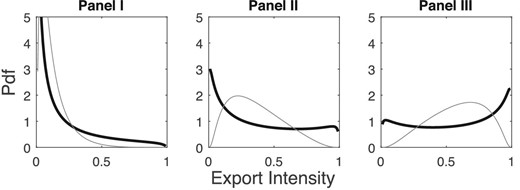
Reduction in export costs with and without twin peaks. The figure plots the pdf of export intensity when revenue shifters are lognormal with |$\sigma ^2_{ zd}+\sigma ^2_{ zx}=4$| (darker line) and |$\sigma ^2_{ zd}+\sigma ^2_{ zx}=1$| (lighter line) for different values of the ratio of scale parameters, namely, |$s_d/s_x=10$| in Panel I, 2 in Panel II, and 0.667 in Panel III.
In Panel I of Figure 6, trade costs are so high that most exporters sell only a small share of their output abroad regardless of the level of dispersion in revenue shifters, and therefore, the two export intensity distributions look quite similar. As trade costs fall, the intensity of all exporters increases, and the distribution of export intensity shifts to the right. However, the difference in the distribution with and without twin peaks also becomes starker. When the variance of revenue shifters is sufficiently large, greater access to foreign markets increases the prevalence of high-intensity exporters moving mass from the left to the right tail of the distribution. In contrast, when dispersion is lower, the increase in the intensity of exporters following liberalization is more gradual.23
Our last theoretical result shows that there is a one-to-one relationship between relative market size and the median export intensity.
See Appendix A.3.
As will become clearer in Section 5 below, this result greatly facilitates the identification and estimation of the parameters of interest.
4.2. Alternative Assumptions
Bimodality of the export intensity distribution can also arise when revenue shifters follow distributions other than lognormal. In Defever and Riaño (2017b), we derive Propositions 1–3 for the distribution of export intensity when revenue shifters are distributed gamma and Fréchet and show that bimodality arises when the dispersion of revenue shifters is sufficiently high.24 Using simulations we find that beta, Chi-squared and F-distributed revenue shifters can also generate bimodal export intensity distributions (although we cannot derive closed-form expressions for the pdf of export intensity in these cases). Pareto-distributed revenue shifters can produce export intensity distributions with two and even three modes.25
So far we have been silent about firms’ selection into exporting when firms face a fixed cost to export, as in the majority of trade models with heterogeneous firms in the spirit of Melitz (2003). Assuming that firms decide whether to export or not only on the basis of their productivity—that is, before the realization of revenue shifters is known—then all our propositions carry through.26 An alternative is that firms make their export decisions based on the realization of both the firm-specific component |$\Phi (\omega )$| and the revenue shifter |$z_x\!(\omega )$|. In this case, for a given level of productivity, only firms with sufficiently high foreign demand choose to export, while only the most productive firms export for a given value of the export revenue shifter. The truncation in the distribution of revenue shifters induced by the fixed cost, however, precludes us from obtaining a closed-form expression for the export intensity distribution. Defever and Riaño (2017a) find that a bimodal export intensity distribution can arise when there is selection into exporting based on productivity and lognormal revenue shifters when solving the model numerically. In Appendix B, we use simulations to show that for a given level of fixed costs, the main message of Proposition 2 still holds true: The distribution of export intensity is bimodal when the dispersion of revenue shifters is sufficiently high.
In Appendix B, we also show that our main result also carries through when revenue shifters are correlated across markets and when firms sell their output in more than two markets.
5. Estimation
In the previous section, we showed that the distribution of export intensity is fully characterized by the sum of the variances of domestic and export revenue shifters and a country’s relative market size with respect to the rest of the world. We now discuss how we estimate these parameters using the cross-country firm-level data from the WBES.
5.1. Identification
The identification of the shape parameter is quite transparent. The value of this parameter is determined by whether the mass of the export intensity distribution is concentrated in the interior of the support or near its boundaries. If the dispersion of revenue shifters is low, then the distribution of export intensity is unimodal with most exporters exhibiting an intensity close to |$s_x/(s_d+s_x)$|. On the other hand, if there were large clusters of exporters with intensities near 0 and 1, then the shape parameter would satisfy the conditions spelled out in Proposition 2. Another convenient feature of (7) is that this measure of relative market size is invariant to the value of the shape parameter. Thus, conditional on relative market size, we estimate country-specific shape parameters by maximum likelihood.27
5.2. Benchmark Estimates
Figure 7 plots the estimated shape parameter for each country against equation (5) from Proposition 2, after having expressed this equation in terms of the median export intensity rather than relative market size using (7). While there is substantial variation across countries, the median export intensity ranges between 0.2 and 0.8 for most of them. For the median country in our sample |$s_d/s_x=1.5.$|, that is, the domestic market is 50% larger than the foreign one. Crucially, all shape parameters satisfy conditions (4) and (5) that ensure the bimodality of the export intensity distribution in every country in our data. Estimates of the two parameters for each country are reported in Table E.1 in Online Appendix E.
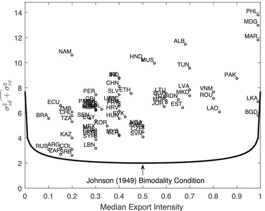
Bimodality condition for lognormal-distributed revenue shifters. The figure plots the lower bound of the condition for bimodality of the distribution of export intensity stated in equation (5) when revenue shifters are distributed lognormal along with the country-specific estimates of |$\sigma ^2_{ zd}+\sigma ^2_{ zx}$|.
The mean estimate for the sum of the variances of revenue shifters across countries is 6.489. This figure falls within the range of estimates for the variance of lognormal firm-destination revenue shifters found by Eaton, Kortum, and Kramarz (2011), and Fernandes et al. (2018) using customs-level data from France and the World Bank’s Export Dynamics Database to estimate structural models richer than ours.28 It is worth noting that their estimates of the variance of revenue shifters are sufficiently large to generate bimodal export intensity distributions in our model.
5.3. Bimodality and Relative Market Size
How can we reconcile the results presented in Figure 7 showing that the distribution of export intensity in all countries is bimodal with those in Figure 5, where we cannot reject the null hypothesis of unimodality for one third of the countries in our data?
We now show that given a sufficiently high variance of revenue shifters, differences in countries’ relative market size vis-à-vis the rest of the world explain both the variation in the distributions of export intensity around the world remarkably well and the reason why the dip test fails to reject unimodality for some countries.
To zero in on the role of relative market size, we assume that firms in all countries draw both of their revenue shifters from a distribution with the same shape parameter. This means that all the variation in the distribution of export intensity across countries is due to differences in their market size relative to the rest of the world. We estimate this “restricted” single-shape parameter model by pooling together data across all countries and weighting each observation by the inverse of the number of exporters in each country to ensure that each country receives the same weight in the estimation.29
The point-estimate for the single shape parameter across all countries is 6.489. This estimate is reported in column (1) of Table 4 and will be our benchmark result. While imposing the same shape parameter across all countries results (by definition) in worse fit to the data than allowing for country-specific shape parameters, the Vuong (1989) test reported in Table E.1 in Online Appendix E, reveals that we cannot discriminate between the full and restricted models in 51 out of 72 countries in our data.30
Different factors accounting for the dispersion in revenue shifters.
| Full sample | Foreign-owned | Excluding | Single-prod. | Countries | |||||
|---|---|---|---|---|---|---|---|---|---|
| Processing | Pure | Old | without ESR | OECD | non-OECD | ||||
| exporters | |||||||||
| (1) | (2) | (3) | (4) | (5) | (6) | (7) | (8) | (9) | |
| Panel A: total export intensity at the country-level | |||||||||
| |$\sigma ^2_{ zd}+\sigma ^2_{ zx}$| | 6.489 | 6.040 | 6.055 | 3.807 | 7.106 | 5.864 | 5.762 | 5.496 | 6.669 |
| (0.050) | (0.053) | (0.051) | (0.033) | (0.096) | (0.070) | (0.070) | (0.111) | (0.056) | |
| Countries | 72 | 71 | 72 | 72 | 58 | 61 | 39 | 11 | 61 |
| Observations | 33,224 | 26,168 | 28,375 | 26,647 | 10,915 | 13,849 | 13,691 | 4,916 | 28,308 |
| Panel B: bilateral export intensity | |||||||||
| |$\sigma ^2_{ zd}+\sigma ^2_{ zx}$| | 8.351 | 8.663 | 7.986 | 3.899 | 15.306 | 7.965 | 7.468 | 11.250 | 6.419 |
| (0.246) | (0.328) | (0.264) | (0.147) | (1.348) | (0.441) | (0.712) | (0.515) | (0.247) | |
| Country pairs | 20 | 15 | 16 | 14 | 3 | 9 | 3 | 8 | 12 |
| Observations | 2,299 | 1,396 | 1,832 | 1,410 | 258 | 652 | 220 | 953 | 1,346 |
Notes. The table reports the maximum likelihood estimate of the shape parameter governing firm-destination-specific revenue shifters, conditional on |$s_d/s_x$| being given by (7). The pdf used in the estimation is given by equation (3). Each firm-level export intensity observation is weighted so that each country receives an equal weight in the estimation. Standard errors are reported in parentheses. Column (1) provides the single shape parameter estimates. Column (2) excludes foreign-owned affiliates (i.e. firms with a share of foreign equity of at least 10%) from the estimation. Column (3) excludes “processing” exporters, that is, firms for which imports account for more than 90% of their total expenditure in intermediate inputs. Column (4) excludes firms with export intensity exactly equal to 1 (pure exporters). Column (5) excludes firms reporting a first export transaction more than 10 years after the year in which they are surveyed. Column (6) excludes firms that export only one product, where a product refers to a 4-digit ISIC industry code. Column (7) excludes countries that provide subsidies subject to ESRs, that is, incentives conditioned on firms’ export intensity exceeding a certain threshold. Column (8) reports the estimate for OECD countries, and column (9) considers non-OECD countries. Panel B reports the maximum likelihood estimate of the single shape parameter of firm-destination-specific revenue shifters conditional on |$s_d/s_x$| being given by (7) using bilateral export intensity data. Each firm-level bilateral export intensity observation is weighted so that each country pair receives an equal weight in the estimation. Among these, column (8) reports the estimate in which the destination country belongs to the OECD, while column (9) considers the case in which destinations are non-OECD countries. Standard errors are reported in parentheses.
Figure 8 presents the fit of the single-shape-parameter model to the data, with countries sorted according to relative market size. Relying only on variation in countries’ relative market size and a unique shape parameter, our model reproduces the wide range of shapes observed in the distribution of export intensity across the world extremely well, with a correlation between the observed and predicted shares of exporters across export intensity bins of 0.88. Crucially, our model is able to generate unimodal distributions where the majority of exporters exhibit either very low or very high export intensity, as well as distributions featuring prominent twin peaks.


Model fit export intensity distribution.
The key is that when a country’s domestic market is either very small or very large relative to the export market (i.e. when the median export intensity is either close to 1 or 0, respectively), the height of the minor mode shrinks so much that the distribution appears unimodal; conversely, in countries in which the size of domestic and export markets is similar, the distribution of export intensity displays prominent twin peaks. Figure 9 illustrates this pattern by plotting the dip statistic calculated for data simulated using the shape parameter reported in column (1) of Table 4 with respect to different values of the median export intensity. Crucially, the dip test fails to reject unimodality when the median export intensity is close to either 0 or 1. Figure 10, in turn, shows that the same inverted-U pattern between the dip test statistic, our proxy for the degree of bimodality of a country’s export intensity distribution, and its median export intensity is clearly borne out in the data as well.
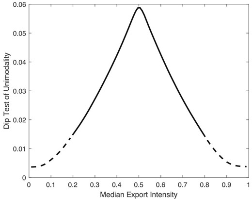
Relative market size and the bimodality of the export intensity distribution, the figure reports the value of the dip test statistic calculated on simulated export intensity draws (2,000 exporters simulated 100 times) using the estimated shape parameter reported in column (1) of Table 4 for different values of the median export intensity. The solid line represents sets of draws for which the null hypothesis of unimodality is rejected at the 1% significance level, while the dashed line shows the realizations for which unimodality is not rejected.
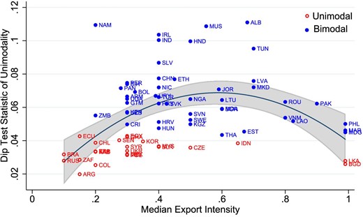
Prevalence of bimodality and median export intensity across countries. The figure plots the fitted values obtained after regressing each country’s dip test statistic (reported in Table 5) on a country’s median export intensity and median export intensity squared. The estimated equation is |${ {dip}} = \mathop {0.0086}_{(0.0096)}\limits + \mathop {0.2044}_{(0.0326)}\limits { {median}} - \mathop {0.1736}_{(0.0397)}\limits { {median}}^2$|, and the shaded area denotes the 95% confidence interval. Hollow circles denote countries for which the dip test does not reject the null hypothesis of unimodality at the 1% level (unimodal), and filled circles indicate countries with a bimodal export intensity distribution (those for which the p-value of the dip test is below 1%).
5.4. Accounting for the High Dispersion of Revenue Shifters
In this section, we re-estimate our single-shape-parameter model excluding the different subsets of observations we defined in Section 3 one at a time. Doing so allows us first to verify that the conditions for bimodality are satisfied in each subsample, and since we are estimating the sum of the variances of revenue shifters, we compare the different estimates in order to gauge the contribution of each group of observations to the benchmark shape parameter estimated using our whole data.
Panel A of Table 4 reports the estimated shape parameter for each distribution and subsample of firms using total export intensity—that is, based on firms’ exports to all destinations divided by total sales—while Panel B uses bilateral export intensity data. We only keep countries (Panel A) or country pairs (Panel B) with at least 50 exporters, and each observation is weighted so that each country or each dyad receives an equal weight in the estimation.
The first conclusion drawn from this exercise is that the estimated sum of the variances of domestic and export revenue shifters remains sufficiently high to generate bimodal export intensity distributions in all cases.31 This result echoes the descriptive findings presented in Section 3. Namely, none of the different firm- and country-level factors we identify as having the potential to generate a substantial share of high-intensity exporters can explain away the twin peaks of export intensity distributions. Remarkably, this result remains true even when we estimate our model using bilateral export intensity (see Panel B of Table 4) and within industries (see Table C.1 in Appendix C). These results allow us to allay the concern that bimodality could be the result of systematic differences in export intensity associated with the number of markets that exporters serve, the specific countries they sell to, or a country’s industry composition.
We next investigate the contribution of each subsample of firms to the estimated overall dispersion of revenue shifters. In most cases, excluding one group of exporters at a time—multinational affiliates, processors, single-product exporters, and exporters located in countries offering subsidies subject to ESRs—results in similar reductions of the sum of the variances of revenue shifters of the order of 7%–11%.32 An alternative, albeit blunt, way to account for policies and other factors that favor exporting relative to selling domestically is to exclude pure exporters altogether from our estimation. Doing so results in the largest impact on the estimated dispersion of revenue shifters, which falls by 42% relative to our benchmark. This is important because if—as our results show—policy distortions account for a substantial share of the dispersion in revenue shifters, then prominent twin peaks could reflect the mis-allocation of firms’ activities across the markets they serve, as Brooks and Wang (2016) show. Crucially, however, the dispersion of revenue shifters we estimate—even when we do away with pure exporters—is still sufficiently high to generate twin peaks.
We also find that the dispersion of revenue shifters is 20% higher among exporters in developing countries compared to those in developed ones. The estimates based on bilateral export intensity further reveal that twin peaks are more prominent among exporters selling to OECD countries than among those selling their output to other developing markets—for example, Indian firms selling to the US tend to have a higher export intensity than those exporting to China. Pure exporters play a central role in accounting for this difference, as almost half of exporters selling to OECD countries are pure exporters, while they account for only 20% of South–South exporters.
While the results reported in Table 4 show that no single factor can fully account for the dispersion of revenue shifters necessary to engender twin peaks, one could be wary of the substantial overlap between the subsets of exporters we examine—for example, a significant fraction of foreign-owned firms are engaged in processing activities and export all their output. In order to address this concern, we carry out a complementary exercise following Hsieh and Klenow (2009). More precisely, we investigate the extent to which the sum of the variances of domestic and export revenue shifters estimated at the country level in Section 5.2 is related to observable country characteristics. Doing so allows us to assess the extent to which different policy proxies and a country’s level of development jointly contribute to explain the variance of revenue shifters.
Table 5 reports our results.33 Column (1) reveals a negative, albeit weak, relationship between the dispersion of revenue shifters and GDP per capita. The estimates reported in columns (2)–(5) paint a similar picture to the results based on the single-shape-parameter model reported in Table 4. Different proxies for policies that incentivize firms to export a high share of their output explain between 12% and 47% of the cross-country variation in the variance of revenue shifters, with the share of pure exporters operating in a country accounting for the lion’s share of the variation. The estimates in columns (6) show that the significance of GDP per capita dissipates once we control for the availability of subsidies subject to ESRs. The results in column (7), in turn, show that all our proxies for individual policies fostering high-intensity exporters remain significant—even when we consider them jointly and control for countries’ level of development.
Dispersion of revenue shifters and policies.
| |$\sigma ^2_{ zd}+\sigma ^2_{ zx}$| | |||||||
|---|---|---|---|---|---|---|---|
| Dependent variable | (1) | (2) | (3) | (4) | (5) | (6) | (7) |
| Log GDP per capita | –0.224* | –0.051 | 0.104 | ||||
| (1.99) | (0.44) | (1.28) | |||||
| Subsidies with ESR | 0.348*** | 0.320** | 0.177* | ||||
| (3.06) | (2.59) | (1.98) | |||||
| Share of foreign-owned firms | 0.403*** | 0.276*** | |||||
| (2.75) | (2.90) | ||||||
| Share of processing exporters | 0.498*** | 0.216** | |||||
| (4.15) | (2.30) | ||||||
| Share of pure exporters | 0.683*** | 0.526*** | |||||
| (3.44) | (2.84) | ||||||
| Observations | 72 | 72 | 72 | 72 | 72 | 72 | 72 |
| R-squared | 0.050 | 0.121 | 0.163 | 0.248 | 0.467 | 0.122 | 0.617 |
Notes. All variables have been standardized by subtracting the mean from each variable and dividing it by its standard deviation. Robust t-statistics (in absolute value) reported in parenthesis. *Significant at the 10% level; **significant at the 5% level; ***significant at the 1% level.
In summary, the estimation of our model shows that while policies that encourage firms to export a high share of their output account for a substantial share of the high level of dispersion of firms’ sales across different markets, they cannot fully account for the prevalence of export intensity distributions that exhibit twin peaks around the world.
6. Conclusion
In this paper, we have shown that the distribution of export intensity varies substantially across the world. Unlike previous work based on data for a single country, we find that bimodal export intensity distributions—with modes near 0 and 1—are the rule rather than the exception.
We then show that a workhorse two-country model of trade with heterogeneous firms and isoelastic demand can reproduce quite successfully the wide range of patterns that the export intensity distribution displays across countries. The key to do so is to allow firms to differ—substantially—in terms of their domestic and export sales. While our analytical results are derived from an admittedly stylized model, our main message carries through to richer environments.
Estimating the parameters that govern the distribution of export intensity reveals that the dispersion of within-firm heterogeneity in sales across different markets is sufficiently high to generate bimodal export intensity distributions in all countries in our data. We then show that whether a country’s export intensity distribution “looks” unimodal or displays prominent twin peaks is explained by the size of its market relative to the rest of the world. We find that while policies that incentivize firms to export a high share of their output account for a substantial share of the variation in the dispersion of firm-destination revenue shifters, they cannot fully account for the widespread prevalence of twin peaks around the world.
Our findings open up exciting avenues for future research. While we have provided a “snapshot” of the distribution of export intensity across the world, several interesting questions remain to be investigated. How does the distribution of export intensity evolve over time? Is the high dispersion of firms’ sales across destinations stable, or has it changed in response to changes in technology, trade costs, and trade policy? Do the industrial evolution patterns of exporters differ across the distribution of export intensity? Last, but certainly not least, it is of paramount importance to continue making inroads in unpacking the sources of the enormous variation observed in the sales of the same firm across different markets.
Appendix A: Proofs
A.1 Proof of Proposition 1
We use the method of transformations for random variables (stated below) to derive the pdf of export intensity. Since export intensity is a monotone transformation of the ratio of export to domestic revenue shifters in our model, we can use the method of transformations to obtain the pdf of export intensity whenever there is a closed-form solution for the pdf of the ratio of revenue shifters.
Figure A.1 presents some examples of the pdf of export intensity when revenue shifters are distributed lognormal for different values of the relative scale parameter |$s_d/s_x$| and the sum of the variance of revenue shifters |$\sigma ^2_{ zd}+\sigma ^2_{ zx}$|.
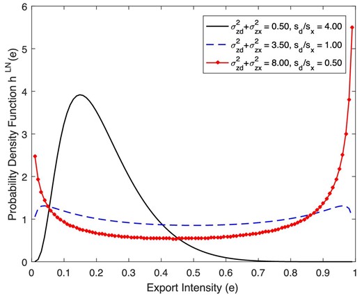
Pdf of the export intensity distribution—lognormal-distributed revenue shifters.
A.2 Proof of Proposition 2
As shown above, the export intensity follows a logit-normal distribution when revenue shifters are distributed lognormal. Johnson (1949) characterized the properties of the logit-normal distribution, which is referred to in his paper as the System |$S_B$| of frequency curves (see equation (23), page 158).
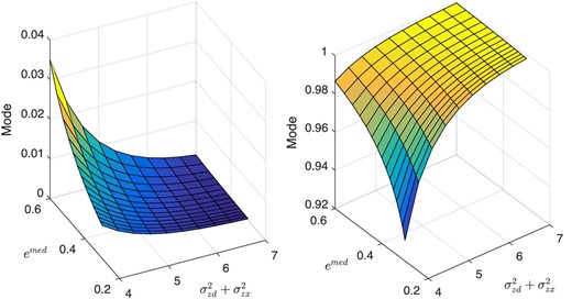
Export intensity modes—lognormal-distributed revenue shifters. The figure plots the two modes of the export intensity distribution (i.e. the solutions to equation (A.11)) as a function of the median export intensity (recall that |$s_d/s_x=(1-e^{{med}})/e^{{med}}$|) and |$\sigma ^2_{ zd}+\sigma ^2_{ zx}$| when revenue shifters are distributed lognormal.
A.3 Proof of Proposition 3
Since the ratio of two independent lognormal random variables is itself a lognormal random variable, it follows that the median of the ratio |$Z_x/Z_d$| is |$z^{ {med}}=\exp [\ln (s_x/s_d)]=s_x/s_d$|.
Appendix B: Discussion of Key Assumptions
In this appendix, we discuss the implications of relaxing different assumptions of our benchmark model for the likelihood of obtaining bimodal export intensity distributions.
B.1 Having More than Two Markets
While there is no closed form expression available for the pdf of the convolution of lognormal random variables, we can still make progress by noting that the sum of independent lognormal random variables can be approximated by a lognormal distribution (Fenton 1960). The Fenton–Wilkinson approximation establishes that the distribution of |$X\equiv \sum _{i=1}^N x_i$|, where |$x_i\sim \mathcal {LN}(\mu _x,\sigma ^2_x)$|, can be approximated by a lognormal distribution with variance |$\sigma ^2_X = \ln (1 + [\exp (\sigma ^2_x)-1]/N)$| and mean |$\mu _X = \ln(N\exp (\mu _x))+ 0.5(\sigma ^2_x - \sigma ^2_X)$|.
Using the Fenton–Wilkinson method to approximate the distribution of total export sales allows us to use Proposition 1 to characterize the distribution of export intensity when the number of foreign markets is greater than 1. The distribution of export intensity is bimodal when the sum of the variance of total export sales and domestic sales is sufficiently large—just as in our two-country benchmark.
B.2 Selection into Exporting Based on Revenue Shifters
Suppose that firms observe the realization of productivity and revenue shifters before deciding whether to export or not. In this case, firms choose to export if the profits from selling abroad exceed the fixed cost of exporting—that is, when |$s_x\cdot \Phi (\omega )\cdot z_x\!(\omega ) \ge \sigma w f_x$|. This condition defines a downward-slopping mapping in |$\lbrace \Phi ,z_x\rbrace$|-space; for a given level of productivity, only firms with sufficiently high foreign demand choose to export, while only the most productive firms export for a given value of the export revenue shifter. The truncation in the distribution of revenue shifters induced by the fixed cost precludes us from using the method of transformations to characterize the pdf of export intensity because the pdf of the ratio of truncated lognormal random variables does not admit a closed-form expression. Defever and Riaño (2017a) find that a bimodal export intensity distribution can arise when there is selection into exporting based on productivity and lognormal revenue shifters when solving the model numerically.
In this section, we use simulations to show that when fixed costs of operation increase, the variance of revenue shifters among exporters is lower than the variance of the (ex-ante) untruncated distribution. Therefore, the distribution of export intensity is less likely to be bimodal as determined by a rejection of the null of the dip statistic. For a given level of fixed costs, however, the main message of Proposition 2 still holds true: the distribution of export intensity is bimodal when the dispersion of revenue shifters is sufficiently high. The main difference relative to our benchmark model is that the dispersion of revenue shifters necessary to generate bimodality increases when selection is present.34
To do so, we draw realizations of productivity, |$\Phi (\omega )$|, and revenue shifters, |$\lbrace z_i\!(\omega )\rbrace _{i\in \lbrace d,x\rbrace }$|, from independent lognormal distributions with mean zero and variances |$\sigma ^2_{\Phi }$|, and |$\lbrace \sigma ^2_{ zi}\rbrace _{i\in \lbrace d,x\rbrace }$|, respectively, for |$N=1,\!000$| firms. We assume that the domestic and export market have the same size, that is, |$s_d=s_x$|, which maximizes the value of the dip statistic—as shown in Section 5.3—and assume that the fixed cost of operation is the same across both markets, that is, |$f_d=f_x=\bar{f}$|. Firms choose to operate in market |$i$| whenever the variable profits in that market exceed the fixed cost, that is, when |$s_i\cdot \Phi (\omega )\cdot z_i\!(\omega ) \ge \sigma w \bar{f}$|. For a given level of fixed costs, we calculate the export intensity and variance of revenue shifters for firms that find it profitable to export (which we refer to below as ex-post variance), and the dip statistic. We set the variance of the log of productivity and the log of revenue shifters equal to each other (reflecting closely the results obtained when we estimate the model’s parameters using sales data, see Defever and Riaño 2017b). We conduct our exercise for two different levels of the variance of log revenue shifters—2.97 and 3.63. These correspond to the median and 75th percentile of the values we estimate for individual countries. We report the dip statistic averaged across 1,000 bootstrapped samples of 500 exporters for each level of fixed costs to ensure that the statistic is not affected by changes in the number of exporters.
Figures B.1 and B.2 present the results of our exercise. When the fixed cost of operation increases, the share of operating firms falls, and the minimum level of revenue shifters necessary for firms to operate (for a given level of productivity) increases. This reduces the ex-post dispersion of revenue shifters, as can be seen in Figure B.2, and therefore, lowers the value of the dip statistic. For a given level of dispersion in revenue shifters, the dip test eventually stops rejecting the null hypothesis of unimodality as the selection mechanism becomes stronger. If the ex-ante dispersion of revenue shifters increases, everything else being equal, the dip statistic increases.

Dip test for different combinations of fixed costs. The figure plots the dip test statistic of unimodality for different levels of fixed costs (and therefore, share of operating firms). Solid lines indicate values for which the null hypothesis of unimodality is rejected by the dip test at the 1% confidence level. Conversely, dashed lines indicate values for which the dip test does not reject unimodality.
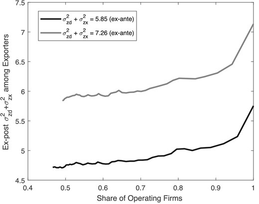
Sum of the (ex-post) variance of revenue shifters among exporters for different combinations of fixed costs. The figure plots the sum of the variance of log revenue shifters among firms that export for different levels of fixed costs (and therefore, shares of operating firms).
B.3 Allowing Revenue Shifters to be Correlated Across Markets
We next investigate the effect of allowing firm-specific revenue shifters to be correlated across markets within a firm. To do so, we take as our starting point our model with two markets and no selection into exporting based on the realization of revenue shifters. We simulate revenue shifters with different combinations of the sum of the variance of revenue shifters and their correlation.35 For each variance and correlation pair, we conduct the dip test of unimodality for the simulated export intensity distribution.
Figure B.3 plots the p-value for these dip tests. It follows that the higher the correlation between revenue shifters is, the higher the sum of the variances needs to be for a bimodal export intensity distribution to arise.
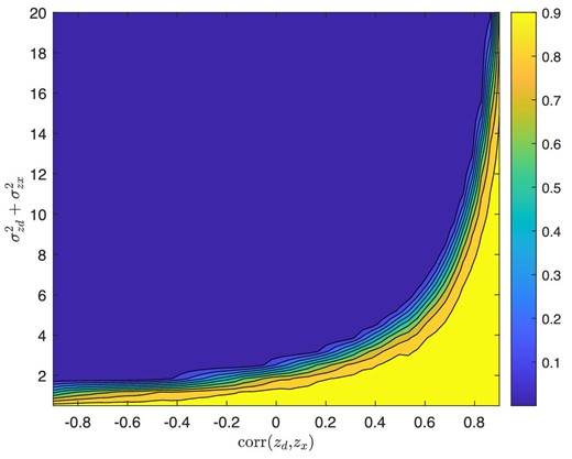
Dip test (p-value) for different combinations of the sum of variance and correlation of revenue shifters. The figure plots the p-value for the dip test for each combination of the sum of the variances of revenue shifters and their correlation. The area in dark blue indicates rejection of the null hypothesis of unimodality, while the yellow area indicates lack of rejection of the null hypothesis.
Under the assumption of independence of revenue shifters, the identification of the sum of their variances is driven by whether the mass of the export intensity distribution is concentrated near the median or the boundaries of the support. Thus, if revenue shifters are positively correlated, then the estimates for the dispersion of revenue shifters necessary to match the export intensity distributions we observe in the data would be even higher. It is important to note, however, that even if we assume that revenue shifters are independent, export and domestic sales can be positively correlated due to the firm-specific component |$\Phi (\omega )$| in equation (1).
In summary, our analysis shows that when the variance of revenue shifters is sufficiently high, then the distribution of the export intensity is bimodal regardless of whether firms can export to many foreign markets, revenue shifters affect firms’ decision to export, or if revenue shifters for firms are correlated across markets.
Appendix C: Shape Parameter Estimates by Industry
Estimated shape parameter—by industry.
| Leather & textiles | Metals & machinery | Food & beverages | Non-metal products | Electric products | Paper & furniture | Chemicals & pharma | Other mfg. | |
|---|---|---|---|---|---|---|---|---|
| (1) | (2) | (3) | (4) | (5) | (6) | (7) | (8) | |
| |$\sigma ^2_{ zd}+\sigma ^2_{ zx}$| | 6.404 | 4.475 | 6.392 | 6.370 | 6.760 | 7.051 | 3.547 | 3.840 |
| (0.137) | (0.174) | (0.253) | (0.440) | (0.377) | (0.503) | (0.236) | (0.258) | |
| Countries | 29 | 14 | 14 | 4 | 4 | 5 | 5 | 7 |
| Observations | 4,368 | 1,327 | 1,277 | 420 | 643 | 393 | 453 | 443 |
Notes. The table reports the maximum likelihood estimate of a single shape parameter for the three distributions of firm-destination-specific revenue shifters conditional on |$s_d/s_x$| being given by (7). Each firm-level export intensity observation is weighted so that each country receives an equal weight in the estimation. The shape parameter is estimated separately for each manufacturing sector. Standard errors are reported in parentheses.
Appendix D: Groups of Countries used in Figure 1
Uppermost panel (Unimodal countries with low export intensity): Argentina, Brazil, Chile, Czech Republic, Ecuador, Egypt, Ghana, Kazakhstan, Korea, Republic, Lebanon, Mexico, Poland, Russian Federation, Senegal, Serbia, South Africa, Syrian Arab Republic, Tanzania, Ukraine, and Zambia (21 countries).
Middle panel (Unimodal countries with high export intensity): Bangladesh, Estonia, FYR Macedonia, Honduras, Indonesia, Kyrgiz Republic, LAO PDR, Madagascar, Mauritius, Morocco, Pakistan, Philippines, Sri Lanka, Thailand, and Vietnam (15 countries).
Lower panel (Bimodal countries): Albania, Armenia, Belarus, Bolivia, Bosnia and Herzegovina, Bulgaria, China, Costa Rica, Croatia, El Salvador, Ethiopia, Guatemala, Hungary, India, Ireland, Jordan, Kenya, Latvia, Lithuania, Malaysia, Moldova, Namibia, Nicaragua, Nigeria, Panama, Paraguay, Peru, Romania, Slovak Republic, Slovenia, Sweden, Tunisia, Turkey, Uganda, Uruguay, and Uzbekistan (36 countries).
Acknowledgments
We thank Giovanni Peri (the co-editor) and two anonymous referees for their constructive comments. We thank Jochen Ditterich, Peter Egger, Julian di Giovanni, Keith Head, Chris Jones, Emanuel Ornelas, Veronica Rappoport, Andrés Rodríguez-Clare, Natalia Ramondo, Dani Rodrik, and seminar participants at Universitat Barcelona, City, University of London, ETH Zurich, LSE/CEP, Universidad del Rosario, the 2015 EIIT conference at Purdue University, the 2016 Royal Economic Society Meetings, the 2016 conference in Industrial Organization and Spatial Economics, St. Petersburg, and the 2017 SED Annual Meetings for their helpful comments and feedback. We would like to thank Facundo Albornoz-Crespo, Salamat Ali, Roberto Alvarez, Paulo Bastos, Carlos Casacuberta, Banu Demir, Ha Doan, Robert Elliott, Mulalo Mamburu, Sourafel Girma, Kozo Kiyota, Balász Muraközy, and Steven Poelhekke for sharing their data or export intensity moments with us. All remaining errors are our own. Defever is a Research Fellow of CESifo. Riaño is a Research Fellow of GEP and CESifo.
Notes
The editor in charge of this paper was Giovanni Peri.
Footnotes
In addition to the observation that the majority of exporters in a country sell most of their output domestically, this body of work has identified two stylized facts that have proven to be very robust across countries and over time: (i) within any given country or industry, exporters are a minority; (ii) exporters outperform non-exporters across a wide range of performance measures such as size, productivity, capital-, skill-, and R&D-intensity (Bernard et al. 2007; Melitz and Redding 2014).
Models in which firms only differ in terms of their productivity are at odds with the wide range of patterns presented in Figure 1. In the two-country model version of the Melitz (2003) model, the share of revenues accounted for by exports is the same for all exporters in a country—that is, the distribution of export intensity is degenerate. With more than two countries, more productive firms have a higher export intensity than less productive ones because the former serve more markets than the latter. The multi-country version of the Melitz model cannot generate right-skewed or bimodal export intensity distributions if the distribution from which firms draw productivity is such that a small number of large firms coexist alongside a large number of small firms (see Simon and Bonini 1958; Axtell 2001). The positive correlation between productivity and export intensity also arises in the Melitz and Ottaviano (2008) two-country model with quasi-linear utility. This again implies that the distribution of export intensity inherits the properties of the productivity distribution.
While our analytical results are derived from an admittedly stylized two-country model, in Appendix B we show that high dispersion in firms’ sales across markets also generates bimodality in models with multiple export destinations when revenue shifters affect firms’ selection into exporting and when revenue shifters are correlated across markets. Our decision to use a two-country model is also driven by the fact that our data has only information on firms’ domestic sales and total exports (we only observe exports by destination for a small number of countries and destinations). The World Bank’s Exporter Dynamics Database, used by Fernandes et al. (2018), provides information on firm-destination-level exports for 70 countries, but unfortunately does not have information on domestic sales nor can it be matched with WBES.
We have also estimated relative size directly from data on firms’ domestic and foreign sales to allay the concern that the transformation of the median export intensity implied by our model might not provide a good approximation to relative market size (Defever and Riaño 2017b). Reassuringly, the correlation between both measures of relative market size is very high.
More specifically, the survey includes formal (registered) firms with more than five employees that are not 100% state-owned. A new survey wave is usually conducted in each country every 3–4 years.
Since the survey asks firms directly about the percentage of their sales exported, the response is bounded at 100%, and therefore does not capture “carry along” trade—a situation in which firms export goods that they do not produce, and which can generate export intensities greater than 1 (Bernard et al. 2019).
The number of exporters per country ranges from 97 in Ireland to 2,112 in India; on average, 40% of firms surveyed in a given country export some of their output.
We identify countries offering subsidies subject to ESRs by relying on information gleaned from the “Performance Requirements and Incentives” and “Foreign Trade Zones/Free Trade Zones” sections of the Investment Climate Statements produced by the US State Department, following Defever and Riaño (2017a).
Díaz de Astarloa et al. (2013) and Heid, Larch, and Riaño (2013) find that high-intensity exporters are larger than domestic firms and other exporters in Bangladesh and Mexico, respectively. On the other hand, Defever and Riaño (2019) document that firms that export all their output in China, although larger and more productive than domestic firms, are smaller and less productive than low-intensity exporters.
For survey waves between 2002 and 2005, we identify these firms by using the question “How many products does your establishment produce?”; in latter survey waves, we consider a single-product exporter as a firm answering the question “what were this establishment’s two main products (as represented by the largest proportion of annual sales)?” with 100% for its main product. This information is available for 70 out of the 72 countries in our original sample and for 71% of exporting firms.
The information on the first year a firm starts exporting is available for 74% of the exporters and for 71 out of 72 countries in our sample.
The countries of origin for which this information is available are Bangladesh, India, Madagascar, Malaysia, Mauritius, South Africa, and Thailand. The destination markets include Australia, China, Indonesia, Japan, Singapore, Thailand, the European Union, the United Kingdom, and the United States.
It is important to note that there is a substantial degree of concentration of exporters across country-sector pairs. One third of exporters in our sample sell textile garments and leather products, while food, beverages, and metal and machinery industries account for approximately 15% of exporters each. About half of Eastern European exporters operate in the metals and machinery industry, while leather and textiles exporters account for more than 40% of exporters in several Latin American and South and East Asian countries.
The dip test has been widely used in economics to, among other things, identify convergence clusters in the distribution of GDP per capita, total factor productivity, and other indicators of economic growth (Henderson, Parmeter, and Russell 2008), characterize the degree of price stickiness (Cavallo and Rigobon 2011) and to assess the identification of hazard function estimates (Heckman and Singer 1984).
More precisely, the cdf of a unimodal distribution is convex on the interval |$(-\infty ,x_m)$| and concave between |$(x_m,+\infty )$|, where |$x_m$| denotes the mode of the distribution.
Hartigan and Hartigan (1985) choose the uniform distribution as the distribution under the null hypothesis because its dip is the largest among all unimodal distributions.
This is a result of the WBES surveys asking firms directly what their export intensity is.
The choice of countries for this exercises was driven by data availability. The manufacturing surveys that we rely upon for the comparison have been used in many prominent papers in international trade, including—but not limited to—Bustos (2011) (Argentina), Alvarez and López (2005) (Chile), Feenstra and Hanson (2005) (China), Roberts and Tybout (1997) (Colombia), Békés and Muraközy (2012) (Hungary), Goldberg et al. (2010) (India), Javorcik and Poelhekke (2017) (Indonesia), Ali, Kneller, and Milner (Forthcoming) (Pakistan), Mamburu (2017) (South Africa), Cole, Elliott, and Virakul (2010) (Thailand), Casacuberta and Gandelman (2012) (Uruguay), and Ha and Kiyota (2014) (Vietnam).
Revenue function (1) obtains in a broad range of setups. For instance, if there is a representative consumer with Constant Elasticity of Substitution (CES) preferences |$\mathcal {U}=\left[\sum \nolimits _{i\in \lbrace d,x\rbrace }\left(\int _{\omega \in \Omega _{i}} [z_{i}(\omega )^{\frac{1}{\sigma -1}}q_{i}(\omega )]^{\frac{\sigma -1}{\sigma }}\text{d}\omega \right)\right]^{\frac{\sigma }{\sigma -1}}$|, where |$\sigma$| denotes the elasticity of substitution between varieties, |$q_i\!(\omega )$| is the quantity of good |$\omega$| from country |$i$| consumed, and |$\Omega _{i}$| is the set of varieties produced in market |$i$| available to consume. In this case, |$z_i\!(\omega )$| denotes the weight with which good |$\omega$| from country |$i$| enters the utility function (see e.g. Crozet, Head, and Mayer 2012; Cherkashin et al. 2015). Alternatively, |$z_i\!(\omega )$| could represent a firm-destination-specific distortion in the variable cost of serving market |$i$|, as in Brooks and Wang (2016), or it could also embody a technology that determines product quality as a function of the firm’s idiosyncratic productivity and the market it intends to sell it to, as in Verhoogen (2008).
|$X$| is a logit-normal random variable if |$Y=\text{logit}(X)=X/(1-X)$| is normally distributed. We thank Chris Jones for calling our attention to this fact.
If both countries are symmetric in size and the reduction in trade costs is bilateral, this direct effect coincides with the full general equilibrium change in relative market size. More generally, a lower trade cost also affects wages and price indices in both countries. Demidova and Rodríguez-Clare (2013) show that it is not possible to unambiguously sign the effect of trade liberalization on wages and price indices in the Melitz (2003) model when countries are asymmetric in terms of size, unless the model is fully parameterized and solved.
To fix ideas, assume that the foreign country is twice as large as home, that is, |$(Y_x/Y_d)(P_x/P_d)^{\sigma -1}=2$| in the context of a standard monopolistic competition model with CES preferences. Then, a |$s_d/s_x$| ratio of 10 (Panel I) implies an iceberg cost of 4.47 (given |$\sigma =3$|). Based on the same parametrization, the iceberg costs in Panels II and III are 2 and 1.15, respectively.
Alessandria and Avila-Montealegre (2020) use the evolution of export intensity in Colombia between 1981 and 2013 to evaluate the roles of trade liberalization reforms and improvements in firms’ exporting technology in accounting for the aggregate increase in the country’s openness to trade.
In the case of Fréchet-distributed revenue shifters, bimodality arises only when their shape parameter is lower than 1, in which case, the expected value of the shifters tends to infinite.
However, similar to the Fréchet case, this only happens when the Pareto shape parameter is lower than 1, and therefore, the expected value of revenue shifters tends to be infinite.
It is important to note that the pdf we derived for export intensity in equation (3) is not defined at an export intensity of 1—that is, it does not admit firms exporting all their output. Since pure exporters are ubiquitous in the data, we need to censor their export intensity, and we do so at a conservative value of 0.99. Using a higher censoring cutoff increases the sum of variances of revenue shifters, thereby biasing the shape parameter of the export intensity distribution in the direction of bimodality. This happens because the distribution of revenue shifters have to generate large shares of extremely low and high realizations to produce a substantial number of exporters with intensity at or above the censoring threshold. To ensure that our results are not driven by our choice of censoring threshold, in Section 5.4 we also re-estimate the shape parameter dropping all pure exporters.
Eaton, Kortum, and Kramarz (2011) estimate the variance of firm-destination specific revenue shifters to be 2.856, while Fernandes et al. (2018) find it to be 6.60. In comparison, if we assume agnostically that the variance of domestic and export shifters is the same, then average variance of revenue shifters would be 3.24.
The WBES also provides an individual weight for each observation depending on firm size, business sector, and geographic regions within a country. The estimates we obtain using the survey’s weights are indistinguishable from our benchmark results reported in column (1) of Table 4 below. These results are available upon request.
Vuong (1989) is a likelihood-ratio (LR) test based on the Kullback–Leibler information criterion. Mrázová, Neary, and Parenti (2021) also use the Kullback–Leibler divergence to evaluate how different combinations of demand functions and productivity distributions fit the size distribution of French firms exporting to Germany. The results of the Vuong (1989) test are reported in Table E.1 in the Online Appendix.
Note that the minimum level for the sum of the variances of revenue shifters to generate bimodality only exceeds four when the median export intensity is below 0.01 or above 0.99—see Figure 7. All the countries in our data lie inside this range, with the exception of Bangladesh, Madagascar, Morocco, the Philippines, and Sri Lanka, all of which have a median export intensity of one.
Although excluding firms that have been exporting for more than 10 years results in an overall shape parameter that is 10% larger than the benchmark estimate.
Note that all variables have been standardized to facilitate the interpretation of the coefficients.
Everything else being equal, a greater dispersion of productivity also helps in generating twin peaks because it lessens the truncation caused by the fixed cost.
We use 2,000 exporters simulated 100 times and assume that the domestic and foreign markets have equal size and, therefore, that the median export intensity is 0.5.
