


Abstract
This paper develops a theoretical framework to study the interaction between globalization and political structure. We show that political structure adapts in a non-monotonic way to declining transport costs. Borders hamper trade. At an earlier stage, the political response to expanding trade opportunities consists of removing borders by increasing country size. At a later stage, instead, it consists of removing the cost of borders by creating international unions. This leads to a reduction in country size. Moreover, diplomacy replaces conquest as a tool to ensure market access. These predictions are consistent with historical evidence on trade, territorial changes, and membership of international unions.
1. Introduction
Since the Industrial Revolution, the cost of distance has been falling dramatically thanks to a stream of major technological innovations like the railroad, the steamship, the telegraph, the jet engine, containerization, and most recently the Internet. Such technological progress has fundamentally transformed worldwide economic geography and fueled a continuous expansion in the size of markets. In 1820, international trade was very modest: about 2% of world output. Over the following century, international trade grew more than four-fold to 8%. This first wave of globalization was cut short in the interwar period, which saw international trade decline to about 5% of world output. After World War II, a second wave of globalization started and still continues today. By 2010, international trade had reached unprecedented levels, surpassing 20% of world output.
These two ages of globalization saw political geography evolve in opposite directions. In the 19th century, economic and political integrations proceeded together. Sovereign states grew larger and fewer, from 125 in 1820 to merely 54 at the eve of the Great War. Conversely, in the post-war era, economic integration has been accompanied by political fragmentation. The number of countries has risen to a record high of more than 190. At the same time, there has been a proliferation of international treaties and institutions aimed especially at fostering economic integration, such as the World Trade Organization and the European Union. These trends are illustrated graphically in Figure 1, which shows the historical evolution of the number of sovereign states in the world and the number of members of the GATT/WTO, along with average exports as a share of GDP.1
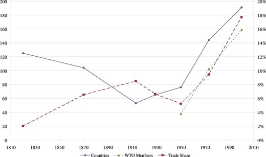
Economic integration and political integration. The figure plots the trade share (right axis), and the number of countries and of WTO members (left axis). See Online Appendix A for details on data.
The sharp reversal in the link between economic and political integrations presents an open puzzle, which we address in this paper. We show that the observed evolution of political structure during both waves of globalization can be understood as an efficient response to the falling cost of distance. Our starting point is that borders hamper trade, so expanding trade opportunities make borders costlier. Political structure needs to adapt by removing borders or by reducing their cost. We find that this adaptation entails a non-monotonic evolution of efficient country size. At an earlier stage, the efficient political response to expanding trade opportunities is to remove borders by creating larger countries. At a later stage, it is to remove the cost of borders by creating international unions. This induces a reduction in the size of countries.
Naturally, our theory does not imply that political geography responds to economic efficiency alone. On the contrary, our model also sheds light on historical patterns of interstate conflict. When creating international unions is too costly, we show that it is appealing for the great powers to wage war to conquer markets. Empire-building enables them to trade with their colonies while imposing extractive institutions. As efficient market size keeps growing, however, we find that this strategy reaches a breaking point. Conflict and imperialism are no longer advantageous for the great powers. They prefer gaining access to world markets through peaceful diplomacy, by building supranational institutions that respect all members’ political autonomy. These theoretical predictions are borne out by empirical evidence. During the first wave of globalization, increasing trade led to an expansion in country size accompanied by conflict. Both links were broken during the second wave of globalization, which saw instead the peaceful rise of supranational institutions.
To derive our results, in Section 2 we set up our model of a world with a continuum of basic geographical units, which we refer to as localities. Each contains people who share common preferences. Goods can be transported at a negligible cost within localities, but at a positive cost across localities. Governments perform two tasks: (i) they enforce contracts, protect property rights, and enact economic regulations that help markets work; and (ii) they provide public services such as education and welfare programs. We study two alternative ways of organizing the government. The first is a single-level government that performs both tasks. We refer to this single-level government as a country. The second possibility is a two-level government. The lower level provides public services and we also refer to it as a country, while the higher level regulates markets and we refer to it as an international union. Our goal is to study how the shape of government changes as the cost of distance declines.
We make two standard assumptions about the effects of government. The first is the presence of border effects. Localities that do not belong to the same country or to the same international union have different economic regulations. Therefore, they can trade only a limited range of goods. The second assumption is policy uniformity. If two localities belong to the same country, then they receive the same basket of public services even though they would prefer different baskets.2
Without costs of government, the optimal political structure would be a two-level government. The first level would be a continuum of country governments, one for each locality, providing each of them with their preferred basket of public services. The second level would be an international union of all localities that regulates markets and eliminates all border effects. Unfortunately, this political structure is too expensive.
We make two standard assumptions about the costs of government. The first is the presence of economies of scale. There are some costs of setting up and running a country that are fixed or independent of the number of localities that belong to it. The second assumption is the presence of economies of scope. Coordinating different levels of government is costly and, as a result, a two-level government is more expensive than a single-level government.
Economies of scale and scope affect the optimal political structure. Economies of scale make it desirable to have a discrete number of countries rather than a continuum of them. Localities are willing to accept public services less than ideally tailored to their preferences in order to benefit from economies of scale. Economies of scope, if large enough, make it desirable to have a single-level rather than a two-level government. Localities may also be willing to accept higher trade costs to take advantage of economies of scope.
The equilibrium political structure balances four classic forces: border effects, preference heterogeneity, economies of scale, and economies of scope. We study how a reduction in the cost of distance affects this balance. Globalization—that is, economic integration—is an endogenous outcome in our theory. An exogenous decline in the cost of distance fosters trade directly for a given political structure. It also fosters trade indirectly by producing endogenous changes in political structure aimed at facilitating trade.
In Section 3, we assume that localities bargain efficiently in a world ruled by law and diplomacy. When trade opportunities are limited, the benefit of creating an international union does not justify sacrificing economies of scope. Thus, a single-level government is optimal. As trade opportunities expand, the incentives to remove borders grow. The number of countries declines, and the mismatch between each locality’s ideal and actual provision of public services grows. Eventually, this mismatch is large enough to justify the move to a two-level government. The world’s political structure shifts from a few large countries to many small countries within an international union. This two-level government is more expensive, but it is nonetheless desirable because it facilitates trade and improves preference-matching in the provision of public services.
In Section 4, we allow a set of core localities to wage war and build empires. War is costly, but it allows core localities to remove borders with their colonies while imposing their preferences on them. Thus, we find that there is an intermediate stage of globalization in which empires are formed. Eventually, this stage ends, empires collapse, and international unions are created to promote trade and peace. Core localities choose to avoid the cost of war and to replace conquered colonies with free partners in an international union. The cause of imperial collapse at a late stage of globalization is the same as the cause of the rise of empires at an early stage: namely, the desire to reap gains from trade in the most cost-efficient manner.
In Section 5, we further relax our assumptions of symmetry and allow core localities to have lower costs of trading with one another. We show that this gives rise to a richer and more gradual pattern of international integration. World-straddling empires are not replaced at once by a world union, but may rather give rise first to a regional union of core localities, which only later grows to encompass the periphery too.
In Section 6, we show three significant patterns in historical data since 1870. First, increases in trade predict territorial expansion before international unions. Second, this correlation is reversed after international unions are created. Third, membership of international unions predicts territorial contraction. This evidence is consistent with the predictions of our theory.
1.1. Related Literature
The motivating facts presented in Figure 1 were first noted by Kahler and Lake (2004) and Lake and O’Mahony (2004). They highlight the puzzling reversal in the link between economic integration and political integration. They stress that it poses an obstacle for efficiency-based explanations of political structure, which have so far failed to account for it and for the emergence of supranational institutions during the second but not the first wave of globalization.
Several economic theories can help explain why economic integration has been accompanied by political fragmentation since World War II (Bolton and Roland 1996, 1997; Alesina, Spolaore and Wacziarg 2000; Casella 2001; Casella and Feinstein 2002). All of them, however, predict a monotonic effect of globalization on political structure, and thus fail to explain why the first wave of globalization was accompanied by a decline in the number of countries. Nor can they explain the creation of international unions. Closest to our own work, Alesina, Spolaore, and Wacziarg (2000) add border effects to Alesina and Spolaore’s (1997) seminal theory of country formation based on the trade-off between preference heterogeneity and economies of scale.3 They explain the increase in the number of countries during the second wave of globalization by interpreting globalization as an exogenous weakening of the border effect. As borders become less costly, the efficient political structure reacts by creating more borders.4
Our model is the first to account for the non-monotonic relationship between globalization and political structure, and to explain the appearance of multi-level governance during the second wave of globalization. We obtain these results because of two innovations relative to prior work. First, we recognize that economies of scope are limited.5 As a consequence, a broader set of political structures can be efficient. Hence, we can explain the shift from a single-level to a two-level government. Second, we consider a more primitive technological driver of globalization: expanding trade opportunities caused by a gradual decline of transport costs, which makes borders costlier. This creates incentives to remove borders rather than to create them. In our theory, the weakening of the border effect occurs only endogenously as the political structure adapts to new trade opportunities.6 This is consistent with O’Rourke and Williamson’s (1999) reading of historical evidence. Trade integration in the 1800s was driven overwhelmingly by declining transport costs, while trade liberalization also became important after the 1950s when it was achieved through international institutions such as the GATT/WTO.
Our work is also related to the literature on trade and war. The idea that trade promotes peace was formalized by Polachek (1980). It is based on the premise that conflict harms trade, and hence trade openness raises the opportunity cost of war (Alesina and Spolaore 2003; Rohner, Thoenig, and Zilibotti 2013). The opposite idea that trade generates military conflict is instead expressed in neo-Marxist theories of imperialism. Trade can also make countries dependent on others and therefore vulnerable (Bonfatti and O’Rourke 2018).7 Our paper suggests that these seemingly antithetical views capture two different stages of the same model. We provide a unified explanation for why territorial changes are more associated with military conflict in the first wave of globalization than in the second, an empirical pattern noted by Lake and O’Mahony (2006). Consistent with our result that international unions remove the market-access incentive for waging war, Martin, Mayer, and Thoenig (2012) find evidence that regional trade agreements promote peaceful relations.
The effect of war on country formation has been studied by Alesina and Spolaore (2003), Griffiths (2014), and Gennaioli and Voth (2015), among others. These papers show that changes in military technology can explain country size, investment in state capacity, and the provision of public goods. However, they find a monotonic effect of military technology on political structure. Our theory also recognizes conflict as one of the determinants of country formation and of the provision of public goods. In our model, waging war is one reason why countries grow large. We show, however, that changes in military technology alone are not sufficient to explain persuasively the observed evolution of political structure. Instead, we find that expanding trade opportunities are key to explain endogenously the creation of international unions along with the switch from a world of aggression in which countries grew large to one of diplomacy in which countries became smaller.
Finally, our work is related more broadly to the economic analysis of federalism and the geographic structure of government. Our model embeds the key trade-off that lies at the heart of the classic theory of fiscal federalism (Oates 1972). Centralization reaps economies of scale and benefits from policy coordination, but it imposes a uniform policy on localities with different preferences. Models of political centralization and decentralization have been applied most often to the architecture of government at the sub-national level (Lockwood 2006; Treisman 2007). However, the same insights apply to the study of international unions (Hooghe and Marks 2003; Alesina, Angeloni, and Etro 2005; Ruta 2005). Prior research in this field has overwhelmingly focused on the optimal size and composition of an exogenously given number of government tiers. Surprisingly, the literature has devoted much less attention to the choice between a single-level and a multi-level governance structure, which our analysis focuses on (an exception is Boffa, Piolatto, and Ponzetto 2016).8
2. A Model of Political Structure
In this section, we develop a stylized model of the world that contains the basic ingredients of our theory: geography, markets, and preferences. The model mixes these ingredients imposing a high degree of symmetry. This allows us to derive our basic results about the effects of expanding trade opportunities on political structure quickly and intuitively.
The concept of locality is a key primitive in our theory. We model the world as a set of places within which there are neither geographical nor cultural distances, and we label them as localities. Thus, localities consist of a group of people sharing common preferences and inhabiting a particular territory. This approach, which is common in the literature, simplifies the study of how people with different preferences interact and organize themselves into political entities. But it is silent about how these different preferences arose in the first place and how they evolve over time. It also abstracts from conflict within localities.
The concept of trade opportunities is another important primitive in our theory. Geographic distance introduces trade costs across localities. In particular, we adopt the usual assumption of iceberg transport costs. We examine the implications of expanding trade opportunities created by an exogenous decline in these costs.
2.1. Basic Setup
Governments provide public services and regulate markets, so government activity affects both welfare components. A political structure for this world consists of two partitions of the set of localities |$[ 0,1]$| into governments: a public-service partition P with a typical element |$P_{n}\in P$|; and an economic-regulation partition R with a typical element |$R_{n}\in R$|.
If |$P=R$|, then we say that the world has a single-level governance structure, and we refer to the common elements of P and R as country governments or countries. Each of these countries provides both public services and market regulation to its constituent localities.
If |$P\ne R$|, then we say that the world has a two-level governance structure. It will presently become clear that governments have a pyramidal hierarchy: if the partitions P and R do not coincide, then the finer partition P is always a refinement of the coarser one R. Hence, we refer to the (smaller) elements of P as country governments or countries, and the (larger) elements of R as international unions or unions. Countries provide public services to their constituent localities, while unions regulate the markets of their constituent countries.
We develop a model of the partitions P and R, that is, a model of how localities organize themselves into countries and how countries organize themselves into unions. We start from assumptions about preferences, technology, and the costs of government, and we determine how welfare |$W_{l}$| depends on political structure |$(P \rm and\, R)$|.
2.1.1. Markets and Trade
To introduce gains from specialization and trade, we adopt a simple symmetric version of the Ricardian model. Each locality is endowed with one unit of labor in each industry. This unit can produce one unit of the variety with the same index as the locality (|$m=l$|), or |$e^{-\eta }$| units of any other variety (|$m\ne l$|). Since |$\eta >0$|, each locality has a technological advantage in its “own” variety. The parameter |$\eta$| measures the extent to which technologies differ across localities and, therefore, the potential gains from specialization and trade.
There are technological barriers to trade. We assume uniform iceberg transport costs across localities so that only a fraction |$e^{-\tau }<1$| of the goods shipped from l to |$m\ne l$| arrives to destination. To focus on the most interesting case in which trade costs are not prohibitive and to ensure positive gains from trade, we assume that |$\eta >\tau >0$|. Our measure of trade opportunities is the wedge |$\gamma =\eta -\tau >0$|, which captures the potential gains from trade. This wedge increases as improvements in transportation technology reduce physical trade costs |$\tau$|. Trade opportunities can thus range from |$\gamma =0$| when trade costs are prohibitive (|$\tau =\eta$|) to a maximum of |$\gamma =\eta$| when trade costs are nil (|$\tau =0$|).
Policy-induced barriers to trade (i.e. border effects) arise when different governments regulate markets. Specifically, we assume that exchanging goods in a fraction |$\beta \in ( 0,1)$| of industries requires legal enforcement of contracts. In these industries, varieties cannot be traded between localities that have different governments regulating their markets, that is, those that belong to different elements like |$R_{n}$| and |$R_{n^{\prime }}$|. The reason is that foreigners correctly anticipate that domestic courts will discriminate against them ex post. In the remaining set of industries, contracts are self-enforcing, and thus varieties can be traded without restrictions. This formulation captures a simple yet realistic microfoundation for the well-known finding that borders obstruct trade.9
2.1.2. Governments
We now introduce three assumptions about governments. The first assumption is about preference heterogeneity. Each locality has a different ideal variety of public services. We define and order the basic varieties such that the ideal one for locality l is |$x=l$|. We assume that |$\delta _{l}( x) =\delta >0$| if |$x=l$|; and |$\delta _{l}( x) =0$| otherwise.
The second and third assumptions define the cost function K. First, there are economies of scale in the provision of public services. Building and maintaining a government reduces the utility from public services by a fixed total amount |$\phi >0$|. This cost is equally shared among the constituent localities. Second, there are economies of scope across government functions. Membership of a union reduces the utility from public services by an amount |$\kappa >0$|. This captures the costs of oversight and coordination between a country and the union.
To complete the model, we need to make assumptions on how localities interact. We consider law and diplomacy in Section 3, and war and conquest in Section 4. In both cases, the world’s political structure is determined by the interplay of the forces that follow from our assumptions. Although these assumptions are standard in the literature, we provide some additional discussion of them in Online Appendix B.
3. Law and Diplomacy
3.1. Equilibrium Political Structure
Equation (11) implies that the equilibrium political structure features either |$P=R$| or |$P\ne R=\lbrace [ 0,1] \rbrace $|. In the first case, the world is organized in a single-level governance structure with a set of countries that provide public services and regulate markets. In the second case, the world is organized in a two-level governance structure with countries providing public services and a world union regulating markets.11
3.2. Globalization and Political Structure
With these results at hand, we can return to Figure 1 and ask again: Why did the first wave of globalization reduce the number of countries but not generate unions? Why did the second wave of globalization increase the number of countries and lead to the creation of unions? To answer these questions, we consider a gradual increase in trade opportunities |$\gamma$| from 0 to |$\eta$|, and we study how political structure changes as this process unfolds.
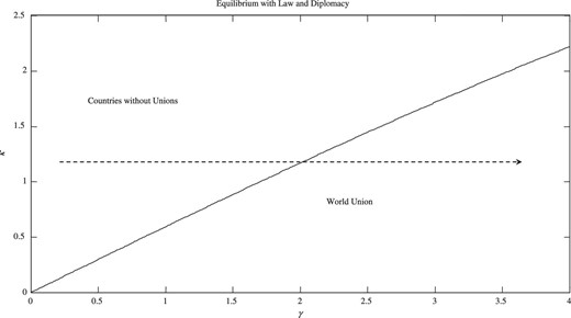
Globalization and political structure. The figure shows how equilibrium political structure depends on economies of scope (|$\kappa$|) and trade opportunities (|$\gamma$|).
Figure 3 displays how political structure changes along the trajectory shown by the dashed arrow in Figure 2, by plotting the equilibrium size of countries and unions as a function of trade opportunities (|$\gamma$|). In the first wave of globalization (|$\gamma <\gamma _{U}$|), it is too expensive to create a world union, so increases in |$\gamma$| lead to an increase in country size. The cost of reaping additional gains from trade is a growing preference mismatch. Eventually, the preference mismatch has grown so large that it becomes cost-effective to create a world union. In the second wave of globalization (|$\gamma >\gamma _{U}$|), the cost of reaping additional gains from trade is the loss of economies of scope. The creation of a world union allows countries to revert to a smaller size and reduce the preference mismatch. Further increases in |$\gamma \,$|have no effect on the equilibrium political structure.
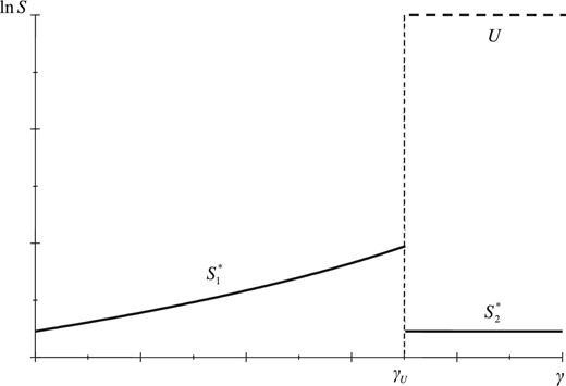
Globalization, countries, and unions. The figure shows how the world political structure changes with trade opportunities (|$\gamma$|). The solid line is the size of each country, and the dashed line is the world union.
The pattern we derive as a consequence of declining transport costs is borne out by historical evidence on the two waves of globalization. In our theory, before the creation of international unions, countries’ borders imposed constant trade frictions (equal to the border effect |$\beta$|). Consistent with this prediction, O’Rourke and Williamson (1999) argue that the first wave of globalization was driven overwhelmingly by declining trade costs and not by the liberalization of cross-country trade. In our model, the creation of international unions endogenously eliminates the trade frictions created by country borders between their members. Consistent with this notion, O’Rourke and Williamson (1999) also suggest that trade liberalization became important after the 1950s—when it was achieved through international institutions such as the GATT/WTO.13
In deriving our results, we have taken transport costs as exogenous. This need not be the case. For instance, the model could be extended by adding the possibility of investing in trade-promoting technologies. Suppose governments can adopt a new technology with a lower |$\tau$|, hence a higher |$\gamma$|, after paying a fixed cost. Suppose also that the new technology, once available, is adopted by all countries. This could be through coordination or simply because new technologies, once discovered, can be copied by others. As we can see from Equation (11), the benefit from improving the trade technology is proportional to the size of countries or unions. Once more, the reason is that the value of lowering trade costs is proportional to the size of the market that is affected. In turn, a better trade technology not only increases the size of countries, but also makes unions relatively more attractive. This suggests the existence of a complementarity between technological globalization and political globalization. The adoption of a better trade technology can trigger the formation of a union. However, the union can also make the adoption of such technology cost-effective. Moreover, the rise of large countries may promote the adoption of trading technologies that could ultimately lead to their collapse. This suggests that the secular increase in trade opportunities need not be a gradual process, but rather can be marked by abrupt changes.
4. War and Conquest
We explore next how war and conquest affect the relationship between globalization and political structure. To do so, we assume that the world is divided into core and periphery. The core contains a measure |$\pi$| of localities with a superior military technology that can be used to conquer other localities and form empires. The periphery contains the remaining localities that do not have this military technology. We keep all assumptions regarding preferences, technology, and the costs of government. Thus, the model of the previous section applies in the limit as |$\pi \rightarrow 0$|.
Empires are an alternative form of government that provides public services and regulates markets. Each empire contains a metropolis and its colonies. The metropolis consists of core localities that unite to conquer periphery localities, which then become their colonies.
Another gain from empire is that the metropolis expropriates market goods from it colonies. We assume it loots a share |$\lambda \in [ 0,1]$| of the colonies’ output in the industries that do not rely on contract enforcement (a share |$1-\beta$| of the total).14 As a result, its consumption of the full measure of varieties in those industries rises to |$c_{l}( m,i) =e^{-\tau }( 1-\lambda +\lambda \int _{0}^{1}I_{l=n}^{E}dn/\int _{0}^{1}I_{l=n}^{M}dn)$|, where |$I_{l=n}^{E}$| is an indicator variable that takes value 1 if localities l and n belong to the same empire and 0 otherwise.
The last benefit of building an empire is that it enables trade in the industries that require legal enforcement of contracts (a share |$\beta$| of the total). The metropolis enjoys the gains from trade creation that result from common market regulation in its empire, while it incurs reduced costs of preference mismatch.
The downside of empire-building for the metropolis is that waging war and holding the empire together reduces the utility that it derives from public services by an amount |$\omega >0$|. This cost captures the diversion of government resources from providing public services in the metropolis to waging colonial wars.
From the perspective of the conquered colonies, instead, the gains from trade creation are dwarfed by the costs of looting and especially of subjugation to an imperial government that generates an unbounded preference mismatch. This division of the surplus captures in our model the extractive nature of imperialism. The metropolis enjoys the gains from trade, while the conquered localities suffer under an exploitative colonial administration.
Periphery localities are incapable of resisting the core’s superior military technology. Thus, a periphery locality remains free if and only if no core locality wishes to colonize it. This may be the case in equilibrium, because each empire has a limited reach. We assume that a metropolis of size M can subjugate a set of colonies of size |$\theta M$|. This assumption captures two considerations. The first is technological. Country size is important for military success, so one of the reasons countries grow large is to prepare for war. The second is ideological. As the disproportion between the size of the metropolis and its colonial targets grows, the aggressive and undemocratic nature of imperialism becomes more obvious, and eventually unpalatable on moral grounds for the citizens of the metropolis. Either force alone suffices for our results.
The equilibrium size of an empire does not depend only on the metropolis’s ability and willingness to use violent repression in its colonies. It is also limited by competition between rival empires, which may clash in an attempt to conquer the same territories. If the sum of desired colonies is larger than the periphery, then empires cannot avoid clashing. We assume that each metropolis can target which periphery localities it tries to colonize. If a periphery locality is targeted by multiple empires, then each of them has an equal probability of colonizing it.
4.1. Equilibrium Political Structure
With war and conquest, the equilibrium political structure need no longer be globally efficient. Formally, the equilibrium political structure is now determined in two stages.
Core localities simultaneously choose whether to build empires and wage wars. Each metropolis chooses which periphery localities (if any) it tries to conquer, taking the choice of other metropolises as given. In the ensuing Nash equilibrium, localities in the periphery may become colonies or remain free.
Localities that do not belong to an empire choose their political structure through efficient bargaining, as in our baseline model.
The world’s equilibrium political structure now consists of a set of empires that have a combined size |$1-F$|; plus two partitions |$( P,R)$| of the free world, which itself has a combined size F. We derive this equilibrium political structure in two steps. First, we determine the political structure of the free world |$( P,R)$| for a given size |$F$|. Second, we determine the number and size of empires and, therefore, the size of the free world F.15
4.1.1. The Free World
The analysis of the free world is essentially the same as in the previous section. The only difference is that now the combined size of the free world is F rather than 1. Efficient bargaining ensures that free localities choose the optimal political structure. Equation (11) still applies and, as a result, there are two cases to consider: |$S=U$| and |$S<U=F$|. The optimal country sizes in these cases are still given by Equations (12) and (13), respectively.16
4.1.2. Empires
Core localities must first decide whether to wage war and build an empire, or to forego war and enter the free world. We start our analysis with three observations. First, a metropolis always targets for conquest all the colonies it can given its own size. Adding extra colonies is desirable from its perspective because it lowers the cost of government, enables looting, and facilitates trade without creating any preference mismatch (for the metropolis) in the provision of public services. Second, in a Nash equilibrium, the overlap between the targets of rival metropolises is minimized. In particular, if the sum of desired colonies is smaller than the entire periphery, then rival metropolises competely avoid clashing with one another. Third, the Nash equilibrium generically features either no empire, or empires whose metropolises span the entire core.
Comparing Equation (21) to Equations (12) and (13), we see immediately that empires are larger than peaceful countries. The reason is that the metropolis does not internalize the cost of the preference mismatch it imposes on its colonies; hence, |$\delta \mu$| appears instead of |$\delta$| in the denominator. An intuitive implication is that an empire is larger when its metropolis is smaller relative to its colonies (μ). Hence, empires are smaller if the core is so large (|$\pi$|) that empires clash in equilibrium; or if they are sufficiently democratic they cannot repress a large share of their population (|$\theta$|).
The equilibrium size of empires is also decreasing with preference heterogeneity (|$\delta$|) and increasing with the importance of trade (|$\beta \gamma$|) and with economies of scale (|$\phi$|). These comparative statics are analogous to those for peaceful countries. An empire is distinguished by its extractive institutions, but these determine the equilibrium size of empires only through economies of scale for the imperial government.
When are empires formed? If core localities wage war and build empires, then their welfare is |$W^{E}( E^{\ast })$|. If core localities instead refrain from waging war and choose to form countries and unions by efficient bargaining, then their welfare is |$\max \lbrace W^{F}( S_{1}^{\ast },S_{1}^{\ast }) ,W^{F}( S_{2}^{\ast },1) \rbrace $|.
If instead |$W^{E}( E^{\ast }) \le \max \lbrace W^{F}( S_{1}^{\ast },S_{1}^{\ast }) ,W^{F}( S_{2}^{\ast },1) \rbrace $|, then there is always an equilibrium in which no empires are formed, diplomacy rules and the size of the free world is |$F=1$|. This peaceful equilibrium need not be unique, though. A Pareto-inefficient second equilibrium also exists if |$W^{F}( S_{2}^{\ast },1) \ge W^{E}( E^{\ast }) \ge \max \lbrace W^{F}( S_{1}^{\ast },S_{1}^{\ast }) ,W^{F}( S_{2}^{\ast },1-\pi /\mu) \rbrace $|. In this case, Pareto efficiency requires all core localities to forego empire-building and create a peaceful world union. Yet, if core localities expect other core localities to build empires, their best response is to build an empire themselves. Empire-building is then a coordination failure that lowers the welfare of every locality in the world; but it is also an equilibrium because once it happens there is no incentive for a single core locality to abandon its empire and join the free world.
4.2. Globalization and Political Structure
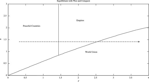
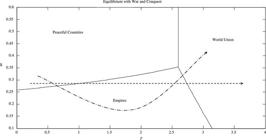
Globalization, conflict, and political structure. The figure shows how equilibrium political structure depends on economies of scope (|$\kappa$|) and trade opportunities (|$\gamma$|).
Figure 5 displays how political structure changes along the trajectory shown by the dashed arrow in Figure 4. At low levels of globalization (|$\gamma <\gamma _{L}$|), the world contains only free countries. There are no empires or unions. As trade opportunities expand, the size of countries grows. When trade opportunities cross the first threshold (|$\gamma _{L}<\gamma <\gamma _{H}$|), core localities prefer to build empires. Empires are larger than countries and keep growing as globalization proceeds. Eventually, trade opportunities cross the second threshold (|$\gamma >\gamma _{H}$|). Empires collapse and countries revert to a smaller size. A world union is created. After this, there are no further changes in political structure.18
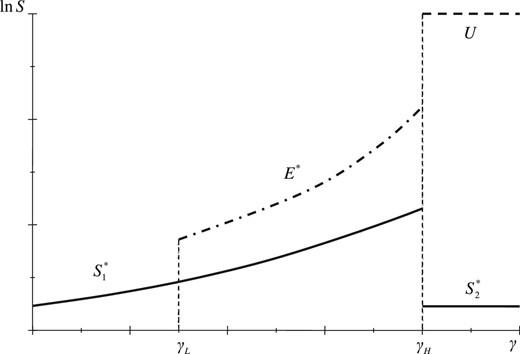
Countries, empires and unions. The figure shows how the world political structure changes with expanding trade opportunities (|$\gamma$|). The solid line is the size of peaceful countries, the dash-dotted line is the size of empires, the dashed line is the world union.
4.3. Other Drivers of Political Structure
Our analysis has focused on growing opportunities for trade as the explanation for the non-monotonic evolution of political structure. However, several additional factors shape the number of countries and the decision to form colonial empires or international unions. A natural question is whether these other factors alone could be driving the patterns we observe in historical data. In particular, could the three-stage evolution of political structure observed in history and depicted in Figure 4 be explained purely by changes in the costs and benefits of war and conquest?
To answer this question, Figure 6 shows how the equilibrium political structure depends on the cost of war (|$\omega$|) as well as trade opportunities (|$\gamma$|). The rise and subsequent fall of empires could be explained by a decline and subsequent increase in |$\omega$| alone, that is, by movements along a vertical trajectory in Figure 6. Such a non-monotonic evolution of the cost of war plausibly fits the historical consequences of advancing military technology. In the 19th century, it enabled the great powers to make easy colonial conquests. Conversely, in the 20th century, it led them to incur horrific costs in two World Wars, and eventually to develop nuclear weapons and the doctrine of mutually assured destruction.
Trade, war, and political structure. The figure shows how equilibrium political structure depends on the cost of war (|$\omega$|) and trade opportunities (|$\gamma$|).
Yet, changes in the cost of war alone cannot explain why what follows empires (international unions) is different from what preceded them (peaceful countries). An expansion in trade opportunities is necessary to account for this pattern. It is also sufficient, as Figure 6 confirms by plotting once again, as a dashed arrow, the straight trajectory along a path of increasing trade opportunities with a constant cost of war. Nonetheless, joint changes in |$\gamma$| and |$\omega$| along a U-shaped trajectory—displayed as a dashed–dotted arrow in Figure 6—paint a more realistic picture. The two drivers of political structure are complementary: changes in the cost of war accelerate the consequences of changes in trade opportunities. In the 19th century, empires arise earlier as conquering colonies becomes cheaper. In the 20th century, international unions arise earlier as war becomes costlier.
This complementarity sheds light on the relationship between peace, trade, and international organizations. In our model, one of the goals of international unions is to reduce the appeal of costly wars. Empirically, this was a key real-world motivation for creating supranational institutions like the United Nations and the European Union. Figure 6 helps understand why they were created only after World War II. By that point, trade opportunities had grown large enough that a positive shock to the cost of war sufficed to trigger a switch from the age of empires to that of peaceful unions.19
The rise and fall of empires may reflect not only the gradual improvement of military technology, but also its gradual spread. Our model captures the traditional view that conflict among rival empires was caused by the spread of industrialization and the attendant rise of new great powers on the world scene. As more localities acquire the technology to conquer empires, the size of the core (|$\pi$|) expands. So long as the core remains small enough (|$\pi <1/( 1+\theta )$|), rival powers can secure their desired colonies without clashing. Accordingly, Britain and France could carve out two world-straddling empires without fighting each other, the Fashoda incident notwithstanding. In this case, the spread of great-power technology increases the number of empires without affecting their size. However, once technology diffusion reaches a critical threshold (|$\pi >1/( 1+\theta )$|), rival powers cannot avoid costly clashes as they try to secure scarce colonies for themselves and deny them to each other. Accordingly, the rise of imperial powers eventually came to be marked by wars like the Spanish–American War and the Russo–Japanese War—and it was arguably a cause of both World Wars.
In our model, such clashes unambiguously reduce the size of the empire each core locality can conquer (|$\partial E^{\ast }/\partial \pi <0$|). At the same time, they force a metropolis to remain relatively large, so as to remain competitive with rivals in the military domain (|$\partial M^{\ast }/\partial \pi >\partial E^{\ast }/\partial \pi$|).20 Intuitively, costly great-power rivalry thus makes imperialism less appealing (|$\partial W^{E}( E^{\ast }) /\partial \pi <0$|). Just as an increase in the cost of warfare, a greater prevalence of clashes between imperial powers (such as the World Wars) hastens the demise of empires (|$\partial \gamma _{H}/\partial \pi <0$|). Once again, though, the simultaneous expansion of trade opportunities is not only a complementary driver of decolonization, but also the factor required to explain the creation of international unions.
Finally, recall that the parameter |$\theta$| can be interpreted as the limit to imperialism arising from moral concerns among citizens of the metropolis. A decline in this limit can represent the spread of democratic values. In our model, a decline in |$\theta$| makes empires weakly smaller (|$\partial E^{\ast }/\partial \theta \ge 0$|) and less desirable (|$\partial W^{E}( E^{\ast }) /\partial \theta \ge 0$|). This effect is always present if the binding constraint on imperialism arises from moral concerns in the metropolis (|$\pi <1/( 1+\theta )$|). If instead the binding constraint is competition between the great powers, the effect only arises if the increase in democratic values is large enough. Since competition between empires grew over time, our theory suggests that democratization may have played a greater role in slowing the rise of empires in the 19th century than in hastening their demise in the 20th century.
5. Regional Unions
Perhaps the most unrealistic aspect of our baseline model is its lack of gradualism. If core localities join a union, then it is a world union. If a world union is created, then country size is reduced at once to its autarky level. However, a simple generalization of our theory shows that this need not be the case. Sometimes, regional unions precede world unions.21
To introduce regional unions, we now consider a slightly richer treatment of geography. Assume that, in addition to having a superior military technology, core localities are closer to each other. Transportation costs for core–core trade are |$\tau -\rho$| (with |$\rho >0$|), so the gains from core–core trade are now |$\gamma +\rho$|. Transportation costs for core–periphery and periphery–periphery trade remain |$\tau$|, so the gains from these types of trade are still |$\gamma$|. The rest of our assumptions remain those of Section 4.
With this additional assumption, a mixed political structure with a two-level governance structure in the core and a single-level governance structure in the periphery becomes possible. Figure 7, which assumes a large enough value for |$\rho$|, shows a scenario in which a four-fold evolution takes place along the trajectory of expanding trade opportunities depicted as usual by the dashed arrow. The first stage is peaceful single-level government everywhere. The second is the creation of colonial empires through which the core conquers and rules distant localities in the periphery. As trade opportunities expand further, empires become overstretched and collapse, and a peaceful union replaces them. The novelty of this third stage is that, unlike in Figure 4, this is now a core union. Indeed, for the most part, in the real world, core countries replaced empires with freer trade not with their former colonies, but with other core countries. Only as trade opportunities expand further a fourth and final stage is reached in which the whole world forms a union.
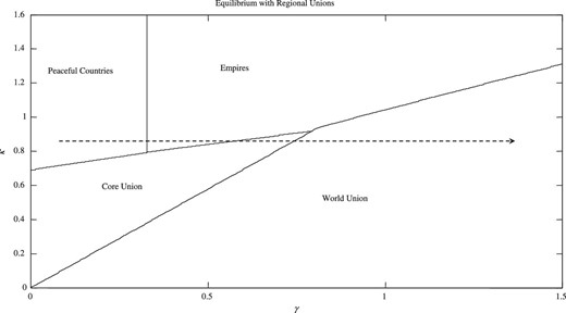
Gradualism and regionalism. The figure shows how equilibrium political structure depends on economies of scope (|$\kappa$|) and trade opportunities (|$\gamma$|).
The model could be further extended in fruitful ways. One extension is a world with two, three, or N peripheries that are located progressively farther away. In this world, there is a union that starts at the core and grows outwardly with expanding trade opportunities. When the first periphery joins the union, the size of its countries declines. When the second periphery joins the union, the size of its countries also declines, and so on. The union gradually advances outward, and it keeps breaking up countries. The end point is the same as in our baseline model, but the world approaches it gradually.
A second extension is a world with two or more core–periphery structures, which we can think of as continents or regions. In this world, within each region, there is one union that advances outward, breaking up countries. Initially, however, no union extends across different regions. Eventually, trade opportunities may expand so much that a world union becomes cost-effective and the regional unions merge. The world approaches the same end point again, but it now approaches it both gradually and regionally.
The bottom line is that asymmetric geography can explain the gradual appearance of international unions with a limited geographic scope. As distance becomes less and less important, the world gradually converges to the single international union we analyzed earlier.
6. Historical Evidence on Trade and Country Size
Our theory provides a new perspective on the connection between trade, country size, and the emergence of international unions. Our motivation for developing this theory was to improve our understanding of global trends, as presented in Figure 1. But the mechanisms that connect trade and country size over time should also be at work when we compare the trajectories of different countries. The extension with regional unions in Section 5 considers trade costs that vary across countries. Moreover, localities could differ in their costs of government, of waging war, and of forming unions. This would introduce heterogeneity in country size and also imply that different countries may join unions at different times.
We exploit such heterogeneity by examining cross-country historical data.22 Our empirical evidence shows that (i) increases in the volume of trade predict increases in country size in the absence of international unions, but (ii) the creation of international unions weakens or eliminates this pattern, and instead (iii) membership of international unions predicts decreases in country size. These findings, though far from conclusive, suggest that the mechanisms our theory highlights are empirically relevant.
6.1. Data
We draw our data from the Cross-National Time-Series (CNTS) Data Archive. This dataset provides information about land area and the volume of trade, measured as the sum of imports and exports per capita, for an unbalanced panel of countries with observations from 1870 to 2010.23
Given that land area changes slowly and discontinuously, we focus on decades and build a dummy variable that takes value 1 if a country or empire has grown in size over the decade. We interpret averages over this variable as the “probability” of a territorial expansion. Similarly, we build dummy variables for territorial contraction that take value 1 if the land area of a country or empire has fallen over the decade. We interpret averages over this variable as the “probability” of a territorial contraction.
Table 1 contains descriptive statistics for the main variables of interest. For each decade, it reports the number of countries with non-missing observations, their average land area, the share of countries that expanded and that contracted their territories, the share of countries that are members of the WTO (GATT before 1995), and the average change in the volume of trade and its standard deviation. Given that all years corresponding to the world wars have no observations in the dataset, the decades around 1940 are missing.
Descriptive statistics.
| Countries | Land area | Expansion | Contraction | WTO | |$\Delta$| trade | ||
|---|---|---|---|---|---|---|---|
| Period | number | mean | mean | mean | mean | mean | std. dev. |
| 1870–1880 | 43 | 738,564 | 0.233 | 0.023 | 0.000 | 0.280 | 0.421 |
| 1880–1890 | 45 | 687,672 | 0.244 | 0.044 | 0.000 | 0.271 | 0.430 |
| 1890–1900 | 46 | 674,440 | 0.217 | 0.109 | 0.000 | 0.084 | 0.303 |
| 1900–1910 | 46 | 670,962 | 0.087 | 0.130 | 0.000 | 0.403 | 0.346 |
| 1910–1920 | 47 | 681,729 | 0.234 | 0.085 | 0.000 | 1.410 | 1.262 |
| 1920–1930 | 55 | 604,987 | 0.164 | 0.073 | 0.000 | 0.466 | 1.041 |
| 1950–1960 | 73 | 536,990 | 0.041 | 0.068 | 0.425 | 0.880 | 0.971 |
| 1960–1970 | 102 | 450,449 | 0.010 | 0.049 | 0.564 | 1.043 | 1.268 |
| 1970–1980 | 127 | 377,772 | 0.024 | 0.055 | 0.591 | 4.613 | 4.504 |
| 1980–1990 | 149 | 274,399 | 0.020 | 0.020 | 0.624 | 0.276 | 0.668 |
| 1990–2000 | 158 | 257,461 | 0.006 | 0.019 | 0.800 | 1.851 | 14.732 |
| 2000–2010 | 169 | 294,461 | 0.006 | 0.012 | 0.845 | 1.698 | 1.327 |
Notes: Countries and land area are measured at the beginning of each decade. Land area is expressed in thousand square miles. Expansion and contraction are dummies taking value 1 if the land area of an existing country expandend or contracted, respectively, over the decade. WTO is a dummy taking value 1 if a country is a member of GATT/WTO at the beginning of each decade.
A quick look at Table 1 confirms the basic trends already discussed. Territorial expansions are much more frequent than contractions in the first part of the sample, but the opposite is true after 1950. The table also reports the average growth in the volume of trade per capita. It shows that trade grows throughout the entire period, but at different speeds both over the decades and across countries.24
Figure 8 shows the average land area of “internationally recognized” countries and of 13 major empires since 1830. The size of empires increases until World War II and falls thereafter. Empires, besides being larger than countries, start reducing their size somewhat later than countries. This picture is consistent with the data on the number of countries shown in Figure 1. Despite the different data sources, both figures tell a remarkably similar story.25 During the 19th century, there was a phase of political concentration in which countries and empires expanded their territories. But this trend was reversed during the 20th century, and especially after World War II.
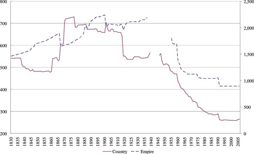
The size of countries and empires. The figure plots the average size of countries (left axis) and of empires (right axis) in thousand square miles. See Online Appendix A for details on data.
Finally, our theory also implies that territorial changes should be associated with conflict during the age of empires but be more peaceful in the era of international unions. Data from the Correlates of War project shows that, indeed, before 1950 more than one third of all territorial disputes involved military conflict, while after that date border changes were peaceful in almost 90% of cases.
6.2. Regression Analysis
We start by studying how the probability of observing a territorial expansion depends on changes in the volume of trade. We perform this analysis by running a series of binomial regressions. To alleviate simultaneity, we compute the change in the volume of trade over the previous decade. Furthermore, to check if the correlation between trade and territorial expansion changes after World War II, we include the interaction between changes in the volume of trade and a post-1945 dummy.
Table 2 reports the main results of estimating a logit model. Standard errors are corrected for clustering by country, to accommodate autocorrelated shocks at the country level. In column (1), we start by including as regressors the lagged change in the volume of trade and its interaction with the post-1945 dummy. As predicted by our theory, the coefficient for the lagged change in trade is positive, the one for the interaction term is negative, and both are highly significant. In other words, trade predicts territorial expansion before World War II, but not after it. In column (2), we also include the post-1945 dummy. The inclusion of the constant and the post-war dummy means that the identifying variation is deviations from the global trends visible in Figures 1 and 8. Nevertheless, the two coefficients of interest remain significant. In column (3), we add year fixed effects, and we keep them in the rest of the table. While these time dummies control for shocks affecting all countries equally, including some common effects of globalization, they do not affect our main results. In fact, the coefficients for the trade variables become even more significant.
Trade and territorial expansion.
| Dependent variable: expansion dummy | ||||||||
|---|---|---|---|---|---|---|---|---|
| All | All | All | All | All | All | Pre-1945 | Post-1945 | |
| (1) | (2) | (3) | (4) | (5) | (6) | (7) | (8) | |
| |$\Delta$| trade | 0.818*** | 0.285* | 0.463* | 0.607** | 0.545** | 0.650* | 0.577** | -0.179 |
| [0.189] | [0.176] | [0.257] | [0.239] | [0.269] | [0.335] | [0.290] | [0.142] | |
| |$\Delta$| trade |$\times$| post-1945 | -1.294*** | -0.287* | -0.580* | -0.896*** | -0.776** | -1.636** | ||
| [0.314] | [0.177] | [0.300] | [0.314] | [0.318] | [0.819] | |||
| Post-1945 | -2.724*** | -5.262*** | -5.626*** | -4.850*** | -2.859 | |||
| [0.472] | [1.242] | [1.566] | [1.353] | [2.405] | ||||
| Log population | 0.595*** | 0.599*** | -2.053 | 0.640*** | 0.460* | |||
| [0.141] | [0.141] | [1.702] | [0.161] | [0.271] | ||||
| Urbanization rate | 0.002 | 0.002* | 0.003 | 0.003 | 0.001 | |||
| [0.001] | [0.001] | [0.004] | [0.002] | [0.002] | ||||
| |$\Delta$| democracy | -0.166** | -0.159 | -0.267** | 0.113 | ||||
| [0.076] | [0.132] | [0.111] | [0.103] | |||||
| Country FE | No | No | No | No | No | Yes | No | No |
| Time FE | No | No | Yes | Yes | Yes | Yes | Yes | Yes |
| Observations | 822 | 822 | 822 | 799 | 651 | 227 | 212 | 439 |
| |$R^{2}$| | 0.0899 | 0.218 | 0.260 | 0.362 | 0.326 | 0.386 | 0.214 | 0.102 |
Notes: All observations refer to 10-year periods. The dependent variable is a dummy taking value 1 if the country’s land area expanded over the decade and 0 otherwise. |$\Delta$| trade and |$\Delta$| democracy are changes over the previous decade. Post-1945 is a dummy for decades after 1945. All other variables are measured at the beginning of each decade. Constant always included and pseudo-|$R^{2}$| reported. Standard errors, clustered by country, are in brackets. *, **, and *** denote significance at 10%, 5%, and 1%, respectively.
We then add some control variables inspired by our model. In column (4), we add the log of population and the urbanization rate at the beginning of each decade.26 The first variable controls for the effect of size, while the second is a proxy for economic development, and both are likely to be correlated with the military strength of a country.27 Both coefficients are positive and significant, but their inclusion does not affect the trade variables. In column (5), we add the change in the level of democracy over the previous decade.28 Consistent with our model and other existing theories, we find that democratization lowers the probability of territorial expansion. Yet, its inclusion has almost no effect on the coefficient for trade. In column (6), we add country fixed effects. This specification is quite demanding: all countries with no changes in size are dropped, and the coefficients are identified only from within-country deviations from country-specific trends. As a result, the sample size falls markedly. Nonetheless, trade and its interaction with the post-1945 dummy are the only two coefficients that remain significant.
Finally, we allow for heterogeneity in all coefficients before and after World War II. To this end, in columns (7) and (8), we split the sample and re-estimate the specifications without country fixed effects separately for the decades before and after 1945. The results confirm that trade predicts territorial expansion in the first part of the sample, but not in the post-war era. As to the remaining coefficients, population has a larger and more significant coefficient in the pre-1945 period, while democracy becomes insignificant after 1945. A possible interpretation of these results is that variables capturing military strength or tolerance for aggression become less relevant when territorial changes are more peaceful. However, the lack of significance may also indicate low statistical power due to the very few territorial expansions observed in the post-World War II period. To study how trade correlates with border changes after 1945, we need to turn to territorial contractions, which have become relatively more frequent.
In Table 3, we run similar binomial regressions to study how the probability of territorial contraction depends on changes in the volume of trade and on being part of an international economic union, measured by membership of the WTO. As in the previous table, the change in the volume of trade is computed over the previous 10 years, the WTO dummy is measured at the beginning of each decade, and standard errors are corrected for clustering by country. We restrict the analysis to the period after 1945, when the WTO dummy starts to have positive values, but results are similar if earlier decades are added.29 In column (1), we include the lagged change in the volume of trade and the WTO dummy. Only the coefficient for the latter is positive and precisely estimated, indicating that countries joining the WTO have a higher probability of a subsequent territorial contraction. In column (2), we add the interaction between changes in trade and the WTO dummy. The coefficient for trade turns positive and become statistically significant. When we add year fixed effects, in column (3), the negative coefficient of the interaction term also become significant. Growth in trade is followed by a higher probability of territorial contraction, but not after a country joins the WTO. This finding suggests that the negative effect of trade on country size may be mediated by membership of international unions like the WTO, as our theory predicts.
Trade, unions, and territorial contraction.
| Dependent variable: contraction dummy | ||||||
|---|---|---|---|---|---|---|
| Post-1945 | Post-1945 | Post-1945 | Post-1945 | Post-1945 | Post-1945 | |
| (1) | (2) | (3) | (4) | (5) | (6) | |
| |$\Delta$| trade | -0.003 | 0.097* | 0.146*** | 0.105** | 0.104** | 0.080 |
| [0.011] | [0.055] | [0.051] | [0.052] | [0.052] | [0.058] | |
| WTO | 1.555** | 1.594** | 2.120*** | 1.744** | 1.785** | 2.423** |
| [0.724] | [0.760] | [0.754] | [0.884] | [0.886] | [1.139] | |
| |$\Delta$| trade |$\times$| WTO | -0.113 | -0.146** | -0.234 | -0.251 | -0.468 | |
| [0.072] | [0.057] | [0.284] | [0.287] | [0.355] | ||
| Log population | 0.503*** | 0.490*** | 0.558*** | |||
| [0.143] | [0.150] | [0.210] | ||||
| Log GDP per capita | 0.549*** | 0.557*** | 0.140 | |||
| [0.188] | [0.205] | [0.412] | ||||
| |$\Delta$| democracy | -0.106 | -0.166 | ||||
| [0.139] | [0.220] | |||||
| Region FE | No | No | No | No | No | Yes |
| Time FE | No | No | Yes | Yes | Yes | Yes |
| Observations | 588 | 532 | 532 | 530 | 486 | 355 |
| |$R^{2}$| | 0.0381 | 0.0318 | 0.155 | 0.248 | 0.239 | 0.255 |
Notes: All observations refer to 10-year periods. The dependent variable is a dummy equal to 1 if the country’s land area contracted over the decade and 0 otherwise. WTO is a dummy for membership of the WTO/GATT. |$\Delta$| trade and |$\Delta$| democracy are changes over the previous decade. All other variables are measured at the beginning of each decade. Constant always included and pseudo-|${}R^{2}$| reported. Standard errors, clustered by country, in brackets. *, **, and *** denote significance at 10%, 5%, and 1%, respectively.
In column (4), we add the log of population and the log of GDP per capita at the beginning of each decade. These proxies for size and economic development, which were associated with territorial expansion before World War II, are now correlated with territorial contraction. This suggests that the countries or empires that were growing before 1940 may be precisely those that started to break up after it. In column (5), we also add the change in the democracy index. While democratization is followed by a lower probability of territorial expansion in the era of empires, it has no statistically significant correlation with territorial contraction after 1950. Adding these controls barely affects the coefficient for the WTO dummy, while its interaction with trade becomes statistically insignificant. Country fixed effects are not feasible because they would shrink our sample size to merely 63 observations. Instead, in column (6), we add region fixed effects. While the estimated coefficient for the change in the volume of trade loses precision, the WTO dummy remains positive and statistically significant. In sum, throughout all specifications, the most robust result is the positive correlation between WTO membership and subsequent territorial contractions.
We have shown three significant patterns in historical data since 1870. First, increases in trade predict territorial expansion before international unions. Second, this correlation is reversed after international unions are created. Third, membership of international unions predicts territorial contraction. To the best of our knowledge, these empirical findings are novel in the literature. While not conclusive, they are remarkably consistent with our theory. The predictions of our model are also consistent with other empirical findings already documented elsewhere. Besides the well-documented trade-creating effect of international unions, of particular interest is Martin, Mayer, and Thoenig’s (2012) finding that regional trade agreements promote peaceful relations between member states.
7. Conclusions
In this paper, we have studied the interaction between globalization and political structure. We have shown that the expansion of trade opportunities can help explain two salient aspects of the evolution of political structure over the last couple of centuries: (i) the rise and subsequent fall in the size of countries observed during the 19th and 20th centuries, and (ii) the seemingly contradictory trends toward more political fragmentation at the national level and more political integration at the supranational level in the second half of the 20th century. We have also provided some historical evidence in support of this claim. Yet, we have deliberately left aside several important factors. We now briefly mention three that seem particularly promising for future research.
First, we have modeled international unions as mere economic agreements to facilitate trade. Although this simplification provides a useful and realistic starting point, it does not do justice to the full political scope of unions, which in reality also provide public goods and coordinate policy choices with cross-border consequences.30 Hence, supranational policymaking involves distributive conflict that we have abstracted from, and which can help explain gradual changes in union membership.
Second, our concept of locality abstracts from internal heterogeneity in both preferences and economic attributes. Yet, historical experience suggests that internal conflict has played a role in the process of country formation and break-up (Bolton and Roland 1996, 1997). It would be interesting to explore how expanding trade opportunities also affect political structure through their effect on domestic heterogeneity and conflict. We know, for instance, that international unions may exacerbate domestic conflict and shape political preferences (Gancia, Ponzetto, and Ventura 2020).
Finally, we have focused on the economic aspects of globalization: an expansion of trade opportunities and how political structure adjusts to take advantage of them. Yet, there are also cultural aspects of globalization, which may entail, for instance, a reduction in preference heterogeneity. Exploring the simultaneous effects of both economic and cultural drivers of globalization on political structure seems a fruitful avenue for further research.
Acknowledgments
We thank Janko Heineken, Marta Santamaria, and Jagdish Tripathy for excellent research assistance. We are grateful for helpful comments by Giovanni Andreottola, Pablo Beramendi, Graziella Bertocchi, Alessandra Bonfiglioli, participants at numerous conferences and seminars, the editor, Giovanni Peri, and four anonymous referees. We acknowledge financial support from the European Research Council under the European Union's Horizon 2020 research and innovation program (StG-240989-GOPG, AdG-693512-GEPPS and StG-714905-CITIZINGLOBAL); the Agencia Estatal de Investigación (MCIN/AEI/10.13039/501100011033: RYC-2013-13838, SEV-2015-0563, CEX2019-000915-S and PID2019-111691RA-I00); the Generalitat de Catalunya through CERCA, the Institut d'Estudis Autonòmics and the SGR Programme (2014-SGR-830 and 2017-SGR-1393); and the Leverhulme Trust through a 2019 Research Fellowship.
Notes
The editor in charge of this paper was Giovanni Peri.
Footnotes
The data on the number of states are from Butcher and Griffiths (2013). The trade share is from Maddison (2001). See Online Appendix A for more details.
We assume that local preferences differ with respect to public services but not economic regulations. Market-enabling economic regulation aims primarily at increasing efficiency, and this goal is widely shared by people with different preferences (Coase 1960; Posner [1973] 2014). Accordingly, government functions such as contract enforcement, monetary policy, or the policing of anti-competitive practices are often entrusted to non-partisan experts. Public services, however, are a focus of political tension because people have different views on how children should be educated, on the proper size and scope of the welfare system, and so on. Such preferences vary systematically across localities reflecting their distinctive history and culture.
Desmet et al. (2011) calibrate this trade-off for European countries.
Bolton and Roland (1996, 1997) focus on income distribution and find that heterogeneous countries may break up if their barriers to external trade decline. Casella (2001) and Casella and Feinstein (2002) study how preferences for public goods can endogenously become more heterogeneous as market size expands and enables greater specialization.
Alesina and Spolaore (2003) offer an insightful discussion of economies of scope. Chapter 2 analyzes an arbitrary system of overlapping jurisdictions. Chapter 9 presents a system of overlapping jurisdictions constrained to form a pyramidal hierarchy.
One way to interpret our findings is that, through our two innovations, we provide an explanation of the decline in the border effect that drives Alesina, Spolaore, and Wacziarg’s (2000) results. The reaction to this decline is the same in our model as in theirs: an increase in the number of countries. However, they take the decline as exogenously given. Instead, we show that it is an endogenous consequence of the creation of international unions.
Martin, Mayer, and Thoenig (2008) show that bilateral trade lowers the probability of conflict, but multilateral trade openness decreases dependence on any given country and hence the cost of a bilateral conflict.
Federalism is a way of making public-good provision more efficient by decentralizing it to a sub-national level of government (Oates 1972). We view economic unions instead as a way of making market regulation more efficient by centralizing it to a supra-national level. Intuitively, the two structures may well coexist because they solve different problems. We derive these results formally in Online Appendix D.4, where we present an extension of our model that includes a third, sub-national, level of government.
This microfoundation is analyzed by Broner and Ventura (2011). There are other microfoundations, though. For instance, tariffs and non-tariff barriers are also policies that discriminate against foreigners and limit the range of goods that can be traded.
Throughout, we disregard the constraint that the number of countries and unions, |$1/S$| and |$1/U$|, must be a natural number. In Online Appendix C.2, we introduce this integer constraint and show that the equilibrium political structure remains symmetric and qualitatively analogous to the tractable approximation we use in the main text.
We know that, if |$P\ne R$|, then there is only one world economic union because the marginal cost of adding members is constant, and the marginal benefit is growing with the size of the union. Thus, having many small unions is not optimal.
Equation (12) assumes that |$\delta >\phi +\beta \eta$|, so there is enough preference heterogeneity to ensure that each country is always smaller than the whole world.
It is instructive to compare our results to Alesina, Spolaore, and Wacziarg’s (2000) finding that expanding trade opportunities always reduce country size. Their analysis differs from ours in two crucial ways. First, they assume prohibitive economies of scope (in our model, |$\kappa \rightarrow \infty$|), so the world always has a single-level governance structure. Second, they model expanding trade opportunities as an exogenous reduction in the border effect (in our model, a decline in |$\beta$| with constant |$\gamma$|). Such a reduction always reduces country size, so their model can explain why the second wave of globalization led to smaller countries, but it cannot explain why the first wave of globalization led to larger countries.
This assumption simplifies the algebra, but our results remain qualitatively unchanged if we assume that looting can take place in all industries, as we show in Online Appendix D.1.
For simplicity, we do not consider the possibility that empires could be members of international unions. Online Appendix D.2 shows that our results are robust to relaxing this assumption.
We now assume that |$\delta >\phi F^{-2}+\beta \eta$| to ensure that countries are always smaller than the free world.
Equation (21) assumes that |$\delta \mu >\phi( \mu /\pi ) ^{2}+\beta \eta$|, so there is enough preference heterogeneity to ensure that the metropolis is smaller than the whole core and a fortiori the empire is smaller than the whole world.
Figure 5 depicts the case in which, during the age of empires, the free world always adopts a single-level governance structure and the shift to the two-level governance structure coincides with the collapse of empires. This need not be the case. If the size of the free world is large enough, an economic union of free countries may co-exist with empires.
Our theory also points to a non-monotonic complementarity between military and trade technologies. In an early stage of globalization (|$\gamma <\gamma _{U}$|), trade-enabling technology (higher |$\gamma$|) complements offensive war technology (lower |$\omega$|). An improvement in either tempts core localities to forego diplomacy and peace and embark instead on imperial conquest, thereby raising the value of an increase in the other. In a later stage of globalization (|$\gamma <\gamma _{U}$|), the pattern switches to complementarity between trade-enabling technology and defensive war technology (higher |$\omega$|), both of which hasten the demise of empires and the advent of peaceful unions. While a dynamic theory of endogenous technological progress remains beyond the scope of our model, these considerations suggest that a realistic U-shaped trajectory in Figure 6 could derive from directed technical change, with causal feedback loops between trading technologies and different types of military technologies.
Great-power rivalry can prove so demanding that an imperial metropolis needs to expand, while its empire shrinks: |$\partial M^{\ast }/\partial \pi >0>\partial E^{\ast }/\partial \pi$| if |$\pi >\max \lbrace 1/( 1+\theta ) ,\sqrt{2\beta \gamma /\delta }\rbrace $|.
An alternative form of gradualism is the creation of unions with increasing depth of international integration. Online Appendix D.3 provides a formalization of this idea.
In a more speculative vein, in Online Appendix E, we provide a brief qualitative narrative showing how our theory helps interpret historical events.
Before 1870, trade data is missing for the majority of countries.
Caution should be taken when comparing some of these variables across decades since the composition of the sample is changing.
Figure 8 is based on the “International System” (Singer and Small 1966), which includes countries with international recognition and reliable data. See Online Appendix A for more details. This classification, however, underestimates the number of independent political entities in the 19th century developing world. Figure 1 is instead based on Butcher and Griffiths (2013), who provide a more comprehensive record.
These variables are also sourced from the CNTS Data Archive. The urbanization rate is the fraction of population living in urban centers of at least 100,000 inhabitants.
More direct measures, such as GDP, are not available for the entire period of analysis.
We use the polity2 index sourced from the Polity IV database. Unfortunately, this index is missing for some of the country-year cells in our dataset.
Before 1950, territorial contractions are infrequent and occur in periphery countries, for which data are scarce and less reliable. If we perform the analysis over the entire sample, then we obtain similar results, but these are driven by the observations after 1950. Hence, adding more decades is not very informative.
