


Abstract
We elicit numerical expectations for late-onset dementia and long-term-care (LTC) outcomes in the US Health and Retirement Study. We provide the first empirical evidence on dementia-risk perceptions among dementia-free older Americans and establish important patterns regarding imprecision of subjective probabilities. Our elicitation distinguishes between precise and imprecise probabilities, while accounting for rounding of reports. Imprecise-probability respondents quantify imprecision using probability intervals. Nearly half of respondents hold imprecise dementia and LTC probabilities, while almost a third of precise-probability respondents round their reports. These proportions decrease substantially when LTC expectations are conditioned on hypothetical knowledge of the dementia state. Among rounding and imprecise-probability respondents, our elicitation yields two measures: an initial rounded or approximated response and a post-probe response, which we interpret as the respondent's true point or interval probability. We study the mapping between the two measures and find that respondents initially tend to over-report small probabilities and under-report large probabilities. Using a specific framework for study of LTC insurance choice with uncertain dementia state, we illustrate the dangers of ignoring imprecise or rounded probabilities for modeling and prediction of insurance demand.
A set of Teaching Slides to accompany this article are available online as Supplementary Data.
1. Introduction
When considering expectations for uncertain events, most economic research maintains that agents hold precise subjective probabilities. Yet some economists have long been concerned that this may not be the case (e.g., Keynes 1921; Knight 1921; Ellsberg 1961), especially when the available information is limited.
This concern has stimulated much research on imprecise probabilities, also known as deep uncertainty or ambiguity; for example, see reviews by Walley (1991), Camerer and Weber (1992), and Marinacci (2015). However, the existing research has largely been theoretical or experimental. Very little is known about the precision of the probabilistic expectations people hold in real life when planning or making decisions with uncertain consequences. The prevalence and nature of imprecision may vary across people and contexts. Hence, we see need to perform empirical research studying broad populations in contexts of substantive importance.
We demonstrate by eliciting subjective probabilities of developing late-onset dementia and future long-term-care (LTC) decisions (purchasing LTC insurance or entering a nursing home), among currently dementia-free respondents in the US Health and Retirement Study (HRS). The HRS is an excellent vehicle for a study of this type, being a major national survey that has elicited probabilistic expectations in the domains of personal health, personal finances, and macroeconomic conditions from older American households since its inception in 1992 (see Juster and Suzman 1995; Hurd 2009).
Our choice to focus on dementia is determined by two main factors. First, dementia is a high-priority topic in the research and policy agendas on aging, due to its increasing prevalence and associated costs (see Hurd et al. 2013; Winblad et al. 2016). Yet expectations of dementia have not been part of the core set of expectations routinely collected in the HRS. Such expectations can potentially affect important economic decisions, including precautionary savings choices, the timing of retirement, and the purchase of LTC insurance.1 Second, we conjecture that many persons may hold imprecise expectations of their dementia risk—and also of LTC outcomes, to the extent that these may depend on dementia expectations. This is because there currently exist no objective personalized predictors of dementia risk, rendering the prediction task difficult for laypeople.2 This is in contrast to other serious illnesses, such as breast cancer and cardiovascular diseases, for which medical researchers have developed easily accessible online tools that predict the chance that persons with specified age and health attributes will develop them. Moreover, existing research on the prevalence of dementia does not provide evidence on the risk that currently healthy persons will develop dementia at some future point in their lives.
To the best of our knowledge, nothing is known about people's beliefs of developing dementia as they age, or about how these beliefs are related to LTC plans and outcomes.3 Our study provides the first empirical evidence about perceptions of late-onset dementia risk and their relationship with LTC insurance plans. We document the prevalence, extent, and heterogeneity of probability imprecision in a national sample of older American households and investigate its implications for analysis of LTC insurance demand.
To do so, we devised an elicitation procedure to distinguish between respondents holding precise probabilities and those holding imprecise probabilities, while also accounting for rounding or approximation of probability reports.4 Our elicitation procedure starts from the precise percent-chance format with which HRS respondents are familiar, which requires respondents to report precise percent chances as numbers between 0 and 100, and then uses two probing questions to learn more about the nature of respondents’ expectations. The first probe asks whether the reported probability was intended to be an exact number or was rounded/approximated. When the response is rounded/approximated, a second probe permits the respondent to give an exact precise probability or an imprecise probability, stated as a range. The question format we develop builds on that used in the exploratory study performed by Manski and Molinari (2010), who posed interval probability questions eliciting longevity expectations from respondents in the American Life Panel (ALP).5 We administered our elicitation procedure in an experimental module that we placed in the 2016 fielding of the HRS.
We find that nearly half of respondents hold imprecise probabilities of developing late-onset dementia. Similar fractions express imprecision regarding purchase of LTC insurance and entering a nursing home. Across LTC and dementia outcomes, over 60% of respondents express imprecision at least once. Respondents with imprecise probabilities vary in the extent of their imprecision, with the distribution of interval widths featuring a median of 20 points and a dispersion of 70 points as measured by the difference between the 9th decile (80 percent) and 1st decile (10 percent). Importantly, imprecision appears to vary with respondents’ conditioning information, with the prevalence of imprecise LTC probabilities decreasing substantially when LTC expectations are conditioned on hypothetical knowledge of the dementia state.
For each outcome, our elicitation procedure generates two measures of subjective expectations as percent chance among respondents who round or approximate their initial report: an initial rounded point probability and a post-probe response, which may be an unrounded point probability or an interval probability. Taking advantage of this data structure, we compare the initial reports that are elicited through the standard HRS format with the reports obtained after our probing questions. When doing so, we view the initial response as a potentially error-ridden measure of the true subjective probability and the post-probe response as a more accurate measure of the truth. As traditional in the measurement error literature, we investigate how the error-ridden measure varies as a function of the underlying true probability.
We find that individuals holding precise probabilities have a tendency, when asked using the standard format, to over-report very small probabilities compared to their post-probing reports. They also tend to under-report large probabilities. A similar pattern is exhibited by respondents holding imprecise probabilities, compared with the lower bound (LB) of the interval that they report post probing, conditional on the width of the interval. About 30% of respondents with imprecise probabilities report an interval that does not include the initial point report.
This pattern, combined with rounding of initial reports by precise-probability respondents, implies that use of initial point-reports for prediction of economic decisions that depend on dementia probabilities can lead to incorrect predictions. We illustrate using a simple model for study of LTC insurance purchase with uncertain dementia state.
Focusing on dementia expectations, we find that HRS respondents hold heterogeneous expectations of developing late-onset dementia, including across education level, age, gender, and ethnicity of the respondent. We study how the prevalence of different probabilistic response types and the amount of probability imprecision vary with observed respondent characteristics. We find that older respondents are more likely than younger ones to report rounded or approximated probabilities and to hold interval probabilities. More educated respondents are less likely to report a rounded or approximated probability, but more likely to hold imprecise probabilities. We find no significant association between probabilistic response type and gender, nor between probabilistic response type and a measure of cognitive ability.
Section 2 reviews the relevant literature and defines the scope of our analysis. Section 3 describes the survey design and data collection. Sections 4 and 5 present our empirical analysis of dementia expectations, with Section 4 studying the imprecision of dementia expectations and Section 5 reporting substantive findings on how respondents perceive dementia risk. Section 6 draws implications of our findings for prediction and modeling. Section 7 concludes.
2. Imprecise Probabilities across Fields
The idea that individuals might not hold precise probability distributions over uncertain events—and, thus, might not make decisions under uncertainty or update their beliefs at arrival of information as Bayesians—has been investigated from multiple perspectives.
The idea appears in economics as early as in the 1920s in the works of Keynes (1921) and Knight (1921). The modern economic literature on decision theory under ambiguity was heavily influenced by the thought experiments and argumentation of Ellsberg (1961). See reviews by Camerer and Weber (1992) and Marinacci (2015).
In statistics, Dempster and Shafer (Dempster 1968; Shafer 1976) developed a generalization of the Bayesian theory of subjective probability, featuring upper and lower probabilities obtained from single independent observations and a rule of conditioning that generalizes Bayesian conditioning. Further efforts followed, sometimes under the nomenclature of robust Bayesian analysis. These include Walley (1991)’s imprecise probabilities framework and Kuznetsov (1991)’s and Weichselberger (2000)’s works on interval statistical models and interval probabilities. Berger (1994) provides an overview of the field.
Manski (2000) connects decision making under ambiguity with problems of identification in empirical research. The reasoning is that ambiguity occurs when lack of knowledge of an objective probability distribution prevents a decision maker from solving an optimization problem. Empirical research seeks to draw conclusions about objective distributions by combining assumptions with observations. An identification problem occurs when specified assumptions combined with unlimited observations drawn by a specified sampling process does not reveal a distribution of interest. Thus, identification problems generate ambiguity in decision making.
Philosophers, too, have developed alternatives to strict Bayesianism. Early examples include the convex Bayesianism of Levi (1974, 1980) and intervalism of Kyburg (1961, 1983). More recent examples include the set Bayesianism of Kyburg and Pittarelli (1992) and other types of imprecise Bayesianism and ambiguity; see reviews by Kyburg and Teng (2001) and Bradley (2017).
The research on imprecise probabilities in philosophy, statistics, and decision theory is largely normative. Our analysis, on the other hand, is descriptive (or positive). Notwithstanding this important difference, our analysis shares with these literatures the idea that imprecise probabilities have the form of probability intervals.
Psychologists and risk analysts have long studied judgement and decision making under uncertainty. Most of this empirical research has focused on precise probabilistic risk perceptions and risk communication (e.g., Morgan, Henrion, and Small 1990; Morgan et al. 2001). However, a group of psychologists have investigated how people use and understand linguistic vis-à-vis numerical expressions of probability in relation to information processing and decision making (e.g., Budescu, Weinberg, and Wallsten 1988; Wallsten, Budescu, and Zwick 1993; Wallsten et al. 1993). Their research has concentrated on the study of experts and of situations where individuals’ knowledge may be imprecise due to stochastic uncertainty and/or linguistic inexactness (e.g., Zwick and Wallsten 1989; Wallsten 1990).
Among economists, the most common approach to carry out empirical research on uncertainty has been to analyze observed or stated choices using the principle of revealed preference, as in structural econometrics or experimental economics. However, multiple combinations of utility, expectations, and choice sets may be consistent with the same observed choices. Hence, strong and often not credible assumptions are required to separately infer preferences and expectations from observed choices.
An alternative is to directly ask individuals. A large economic literature on subjective expectations elicits subjective probabilities from survey respondents using a numerical scale of percent chance. These data have been used to estimate random utility models of choice under uncertainty and to study how individuals form and update expectations in real life. Manski (2004, 2018a), Attanasio (2009), Hurd (2009), van der Klaauw (2012), Armantier et al. (2013), Delavande (2014), Schotter and Trevino (2014), Giustinelli and Manski (2018), Gennaioli and Shleifer (2018), and Altig et al. (2020) trace the developments of the literature from various perspectives and in different subfields of economics and finance.
Most of this literature has maintained that respondents hold precise probabilities and has used subjective expectations data at face value. However, many questions posed in surveys of subjective expectations refer to events over which some respondents might not easily have or be able to form precise probabilities. As discussed in Manski (1993), individuals forming expectations face an inferential problem similar to that faced by econometricians who use prior knowledge and available data to learn features of a probability distribution of interest. Different individuals may possess different data on realized events, may have different prior knowledge of the environment, and may process their information differently. Thus, like econometricians, they may make inferences of differing strength. Like econometricians who determine that available data and credible assumptions only partially identify a distribution of interest, some individuals may not possess sufficient data or prior knowledge to form precise probabilities over certain future events. In line with this reasoning, we conceptualize imprecise probabilities as reflecting limited knowledge and interpret our findings accordingly.
Whereas we assume that persons use imprecise probabilities to express limited knowledge, some researchers have questioned whether persons think in quantitative probabilistic terms at all. In psychology, Zimmer (1983, 1984) argued that humans process information using verbal rather than numerical modes of thinking, and he concluded that expectations should be elicited in verbal rather than numerical forms. In economics, some studies have sought to interpret elicited ordinal and verbal expressions of “confidence” (see Drerup, Enke, and Von Gaudecker 2017; Giglio et al. 2021 for recent examples). These studies do not provide precise or imprecise probabilistic interpretation of this term.
Our interest in the possibility that people may hold imprecise probabilities derives in part from our previous studies of rounding of probability reports by HRS respondents (see Manski and Molinari 2010; Giustinelli, Manski, and Molinari 2020). It has been found repeatedly that survey reports of numerical probabilistic expectations display substantial heaping at multiples of 5 and 10 percent, especially 0, 50, and 100 percent. This data pattern suggests that survey expectations are rounded. Manski and Molinari (2010) hypothesize that respondents may round to simplify communication, a situation compatible with precise probabilities, or to convey partial knowledge, a case consistent with imprecise probabilities.
In our new study, we develop and field a series of probing questions to directly elicit the extent to which individuals round or approximate their responses, whether they hold imprecise probabilities, and, if so, the extent of probability imprecision.
3. Measuring Precise and Imprecise Probabilities
3.1. HRS Experimental Module on Dementia and LTC Expectations
The HRS has been at the forefront of measurement of economic expectations of older US households. From 2002 on, Section P of each biannual wave of the HRS Core questionnaire has elicited expectations on a 0–100 percent chance scale. It poses about 25–35 questions spanning the domains of personal health, personal finances, and general economic conditions, with many repeated across waves.
Additional expectations data have been collected in selected HRS waves and from specific subsets of HRS respondents by means of so-called Experimental Modules.6 For the analysis of this paper, we use expectations data from an experimental module designed by us and fielded in the 2016 wave of the HRS. Being able to field our own experimental module in the HRS is a strength of our data collection effort, which we think strikes a good trade-off between sample size, which could be larger if we used other platforms such as Mechanical Turk, and quality of the sampling scheme, which might be inferior in other platforms.
Our module elicits expectations for future development of dementia, LTC decisions, and their relationship, from a random sub-sample of 1,293 eligible participants in the 2016 wave of the HRS. Module eligibility required that respondents did not live in a nursing home at the time of the survey and had never been diagnosed with Alzheimer’s disease or other forms of dementia. Combined with the fact that HRS respondents are aged 50 and over, these eligibility criteria select dementia-free individuals at risk of developing late-onset dementia as they age. They are effectively no longer at risk of early-onset dementia.
Eligible respondents were randomly assigned to one of two question sequences regarding a distinct LTC outcome: purchasing LTC insurance or entering a nursing home. Overall, each respondent was asked about their expectations for four outcomes: purchasing LTC insurance or entering a nursing home, developing dementia, and purchasing LTC insurance or entering a nursing home if they were to know their true future dementia state (developing dementia, not developing dementia).
Except for the brief description in Section 4.3 and the analysis of Section 6.3 relating expectations of purchasing LTC insurance and dementia expectations, we discuss the LTC questions and analyze responses to them in separate research in progress. This paper focuses on the question asking respondents to report the percent chance of developing dementia in the future.
All respondents taking the module were asked for their expectation of developing dementia. The question was worded as follows:
Q0. Dementia is a general term for a decline in mental ability severe enough to interfere with daily life. Memory loss is an example. Alzheimer's is the most common type of dementia. On a scale of 0 to 100, what is the percent chance that you will develop dementia sometime in the future?
This particular expectation question was never previously asked in the HRS or, as far as we are aware, in any other survey. The question uses the same format as the standard expectation questions in Section P of the HRS Core questionnaire. Respondents are asked to answer with a number between 0 and 100 percent, where 0 means that there is no chance that the event described in the question will happen and 100 means that the event is certain to happen. When a respondent insists that they do not know the chance of the event, their response is recorded as “Don’t know” (DK). If a respondent refuses to answer the question, their response is recorded as “Refuse” (RF).7
Compared to the standard format, the module has a number of distinctive features and measurement innovations. These enable us to provide novel empirical evidence regarding the precision of probabilistic expectations and to shed light on the consequences that heterogeneously imprecise probabilities can have for interpretation of current survey measures of probabilistic expectations in economic surveys.
The first new feature is that each of the four expectation questions in the module is followed by a sequence probing to learn whether respondents were rounding or approximating their initial response and, if so, the extent and reasons for rounding. The purpose of the probing questions is to classify respondents in terms of the precise or imprecise nature of their probabilistic beliefs and also in terms of their tendency to report beliefs exactly or in a rounded form.
We designed three probing sequences, one for each of three types of answer a respondent might give to the expectation question: (i) a numerical point response between 0 and 100 percent; (ii) a numerical interval response such as “between 30 and 60 percent” or “less than 80 percent”; and (iii) a DK response.
Recall that the standard format used in the HRS Core does not allow respondents to answer with an interval. If a respondent happened to answer with an expression conveying a range of chances, the interviewer is instructed to ask the respondent to convert their answer into a single value. On the contrary, in our module, we decided to keep record of “spontaneous” interval responses. In a separate follow-up question described below, we asked respondents to convert their initial interval response into a point response. This approach enables us to learn the range of values that first came to the respondent's mind, alongside the “forced” point response, which would be elicited according to the standard format.
We first describe the sequence of probing questions following a point response to an initial expectation question. Next, we describe the other two sequences, following, respectively, an interval response and a DK response.8
Probing Sequence after a Numerical Point Response
The sequence of follow-up (FU) questions after a numerical point response is structured as follows.
Point FU Q1. When people are asked to give a numerical response, like percent chance, sometimes they give exact answers and sometimes they give rounded or approximate numbers. When you said [X] percent just now, did you mean this as an exact answer or were you rounding or approximating?
Possible answers: exact answer; rounding/approximating; DK/RF.
Respondents indicating that their point response was exact were asked the next expectation question. Respondents indicating that they were rounding or approximating were asked a second probing question.
Point FU Q2. Now please try without rounding or approximating your answer. What is the percent chance that [EVENT] sometime in the future? If you are uncertain about the chances, you may give a range. For example, you may say something like “less than 20 percent,” “between 30 and 40 percent” or “greater than 80 percent.”
Possible answers: a percent chance in 0–100; a closed or open from below/above range; DK/RF.
Probing Sequence after a Numerical Interval Response
Respondents who answered the expectation question with a spontaneous interval response were asked the following probing question before being routed to the next expectation question.
Interval FU Q1. If you had to answer with a single value to the previous question, what point would you give?
Possible answers: a percent chance in 0–100; DK/RF.
Probing Sequence after a DK Response
Respondents who insisted that they did not know the chance of the behavior or state whose expectation they were asked to report were asked the following probing questions.
DK FU Q1. When people are asked to give the percent chance that something will happen in the future, sometimes they give exact answers and sometimes they feel uncertain about the chances. When you said you don’t know just now, did you mean you feel uncertain about the chances or something else?
Possible answers: uncertain about the chances; something else; DK/RF.
Respondents indicating that they were uncertain about the chances were asked a second follow-up question; all other respondents were skipped to the next expectation question.
DK FU Q2. If you are uncertain about the chances, you may give a range instead. For example, you may say something like “less than 20 percent,” “between 30 and 40 percent” or “greater than 80 percent.” If you could give a range, what range would you give to the percent chance that [EVENT] sometime in the future?
Possible answers: a percent chance in 0–100; a closed or open from below/above range; DK/RF.
Figure 1 displays the feasible survey paths following any of the four expectation questions asked in the module: unconditional dementia probability, unconditional LTC probability, conditional LTC probability given no future dementia, and conditional LTC probability given future dementia. The displayed paths are mutually exclusive across alternative initial answers to the expectation question. In general, a respondent might follow different paths when responding to different expectation questions.
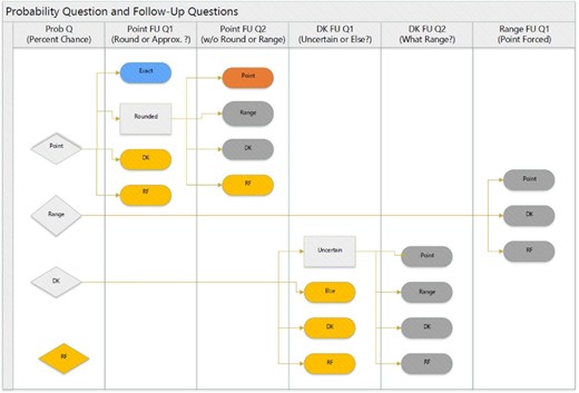
Survey structure and classification of respondents’ probabilities. The figure displays the feasible survey paths following any of the four expectation questions asked in the module (unconditional LTC, unconditional dementia, conditional LTC given no dementia, and conditional LTC given dementia). The displayed paths are mutually exclusive across alternative answers to the initial expectation question, listed in the first panel to the left (from top to bottom: “Point”, “Range”, “Don’t know”, and “Refuse”). For each expectation question, we use the answers to the corresponding follow-up questions to classify respondents’ probabilities into one of four mutually exclusive and exhaustive categories. The follow-up questions are listed at the top of the panels from the second to the left to the sixth and last panel to the right. The probabilities of respondents who gave an exact point response to the initial expectation question are classified as “Exact” (EX). The probabilities of respondents who gave a rounded point response followed by an unrounded point response are classified as “Precise” (PR). The probabilities of respondents who gave a rounded point response followed by an interval or a DK response are classified as “Imprecise” (IM); this category includes spontaneous interval responses and DK responses by respondents who felt unsure about the chances. The probabilities of all remaining respondents are labeled “Other”.
For each expectation question asked in the module, we use the answers to the corresponding probing questions to classify respondents’ responses into one of four mutually exclusive and exhaustive categories. Each category is defined by whether the respondent holds a precise or imprecise probability about the event in question and by whether the respondent reported the probability exactly or as a rounded number. The answers of respondents who gave an exact point response to the expectation question are classified as “Exact point probabilities”. The answers of respondents who gave a rounded or approximated point response followed by an unrounded point response are classified as “Rounded/approximated point probabilities”. The answers of respondents who gave a rounded or approximated point response followed by an interval are classified as “Interval probabilities”. This category further includes the probabilities of respondents who spontaneously answered the expectation question with an interval and of those who answered DK because they felt unsure about the chances. The answers of all remaining respondents are labeled “Other”.
Our design elicits precise and imprecise probabilities by means of a probing sequence that follows the standard HRS question, rather than directly giving the respondent the options of reporting the subjective probability as a single value or a range. We made this choice deliberately, as we wanted to use an elicitation procedure that would start from a format with which HRS respondents were familiar while enabling us to learn about the nature of people's reports. We are aware that this approach might prompt some respondents to think more deeply about the question and, perhaps, to revise their beliefs.9 We carefully chose a neutral wording so as to avoid steering respondents toward reporting intervals over unrounded points or vice versa.
4. Results on Imprecision of Subjective Probabilities Related to Dementia
This section and the next analyze the responses of HRS respondents when answering the dementia question, focusing on imprecision here and the substantive findings in Section 5. In this section, we additionally discuss imprecision of LTC expectations. Our analytic sample consists of 1,255 respondents for whom we have complete and logical responses. We drop 38 respondents whose answers feature illogical values or patterns.
We exploit answers to the probing questions previously described to distinguish cases in which respondents round or approximate their reports, even though they hold precise probabilistic beliefs, and cases where respondents round or approximate to convey imprecise probabilities. We distinguish three groups of persons: those who state that their initial responses were exact numbers, called group Exact (EX); those who rounded/approximated and who reported precise probabilities after probing, called group Precise (PR); and those who rounded/approximated and who reported probability intervals after probing, called group Imprecise (IM).
We assume that the responses that persons give after probing express their true expectations, be they PR or IM. Being unable to directly observe the cognitive processes of respondents, we cannot be certain that this assumption is universally accurate. We use it because we think it to be reasonably valid and because it offers a coherent framework for empirical analysis of the HRS data.
4.1. Patterns of Imprecision
4.1.1. Prevalence and Extent of Imprecision
Column 1 of Table 1 displays the empirical distribution of the three probabilistic response groups and the small remainder who could not be classified. About 49% of the respondents express precise probabilities of developing dementia after probing, and 47% express imprecise probabilities. The latter include a small minority of 6%–7% of respondents who spontaneously gave an interval in response to the initial probability question.10 The response of the remaining 4% of respondents could not be classified due to DK/RF responses to the initial and/or probing questions.
Classification of responses to the dementia probability question into probabilistic response types.
| All respondents | Respondents who gave an initial point response of 0 | Respondents who gave an initial point response of 50 | Respondents who gave an initial response other than 0 or 50 | |
|---|---|---|---|---|
| % Exact point (EX) | 34.8 | 73.3 | 27.9 | 27.1 |
| % Rounded point (PR) | 14.3 | 8.3 | 23.6 | 13.2 |
| % Interval (IM) | 46.5* | 15.5 | 47.6 | 53.9 |
| % Other | 4.4 | 2.9 | 0. 9 | 5.8 |
| N | 1,255 | 206 | 233 | 816 |
Note: N = number of observations.
*The proportion of spontaneous interval probabilities is 6.5%.
Our probing sequence thus reveals that nearly half of the respondents hold imprecise subjective probabilities about future dementia status. These respondents are capable and willing to quantify the extent of their uncertainty by means of a range of percent chance when given the option to do so. Absent this option, as in the standard HRS question format, cooperative respondents tend to report imprecise subjective probabilities as rounded point responses. This evidence is consistent with the hypothesis advanced by Manski and Molinari (2010) that the common tendency of survey respondents to give rounded responses to probabilistic expectation questions may reflect imprecision in their underlying beliefs.
To gauge the extent of the imprecision, Table 2 displays the 1st decile, median, and 9th decile of the empirical distribution of interval widths among respondents with imprecise probabilities. These statistics are shown separately for the large majority who answered the initial dementia question with a point probability and the post-probe question with a probability interval (column 1) and for the small minority of respondents who answered the initial dementia question with a spontaneous interval (column 5).
Width of interval percent-chance responses among respondents with imprecise dementia probability (IM).
| Respondents who gave an initial point response | Respondents who gave an initial point response of 0 | Respondents who gave an initialpoint response of 50 | Respondents who gave an initial response other than 0 or 50 | Respondents who gave an initial interval response | |
|---|---|---|---|---|---|
| 1st decile | 10 | 10 | 10 | 10 | 10 |
| Median | 20 | 20 | 20 | 20 | 20 |
| 9th decile | 80 | 80 | 70 | 80 | 80 |
| N | 442 | 29 | 107 | 306 | 78 |
Notes: Shown statistics refer to respondents reporting a rounded point response followed by an interval (columns 1–4) or a spontaneous interval response followed by a “forced” point (column 5). For each respondent, the interval width is computed as the interval's UB minus the interval's LB. N = number of observations.
Notwithstanding the difference in survey behavior between the two sub-samples of respondents, their empirical distributions of interval widths are quite similar. The median interval width is 20 percent in both sub-samples. The 1st and 9th decile are, respectively, 10 and 80 percent in both sub-samples.
Column 1 of Table 1 shows that, among the respondents who give precise dementia probabilities after probing, 30% report that their initial responses were rounded or approximated. Thus, our probing sequence reveals that the practice of rounding or approximating probability reports in expectation surveys is not limited to respondents with imprecise probabilities. Some respondents may round or approximate their probability reports to simplify communication, as hypothesized by Manski and Molinari (2010).
4.1.2. Focal Responses and Imprecision
Some authors refer to the values 0, 50, and 100 percent as “focal” responses and have advanced specific hypotheses about their meaning. Fischhoff and Bruine de Bruin (1999) and Bruine de Bruin et al. (2002) hypothesize that some respondents use 50 percent to signal epistemic uncertainty, meaning extreme imprecision in beliefs. Lillard and Willis (2001) and Hudomiet and Willis (2013) conjecture that respondents form precise subjective distributions for the probability of an event and then, perhaps to simplify communication, they report whichever of the values (0, 50, 100) is closest to the mode of their distribution. This is termed the “modal response hypothesis”.
Columns 2–4 of Tables 1 and 2 enable us to empirically assess these hypotheses. These columns display the empirical distributions of probabilistic response types and of interval widths for respondents who answered the initial probability question with the value 0 percent, 50 percent, or an answer other than 0 and 50 percent. We do not separately report the distributions for respondents who initially answered 100 percent because less than 1% of respondents did so.
We find that respondents who initially gave a response of 0 percent are much more likely than others to report after probing that their response is exact, less likely than others to report that their response is a rounded or approximated point probability, and much less likely to provide a probability interval. These results are contrary to the modal response hypothesis, which conjectures that responses of 0 percent tend to reflect substantial rounding.
Respondents who initially gave a response of 50 percent are equally likely as most others to report that their response is exact, more likely to report that their response is a rounded or approximated point probability, and slightly more likely to give an interval when permitted to do so. These results are inconsistent with the epistemic-uncertainty hypothesis, which conjectures that responses of 50 percent tend to reflect substantial imprecision in beliefs. The pattern of the interval-width distributions across subsamples shown in Table 2 further supports no differential imprecision of dementia probabilities between respondents who initially answered with 50 percent and those who answered with numbers other than 50.
4.1.3. Variation of Imprecision with Observed Respondent Attributes
We conclude this initial description of findings by investigating how the prevalence of different probabilistic response types and the amount of probability imprecision vary with observed respondent characteristics. To this end, we first estimate multinomial probit regressions of probabilistic response type as a function of respondent age, gender, race, and education. Another specification adds an HRS measure of cognition. The estimates are reported in Online Appendix Table S1. Next, we estimate mean linear regressions of interval width conditional on the same vectors of covariates among respondents with imprecise dementia probabilities. These estimates are reported in Online Appendix Table S2. Here, we summarize the findings in Online Appendix Table S1. See the Online Appendix for further discussion of these findings and those in Online Appendix Table S2.
We find that older respondents are more likely than younger ones to report rounded or approximated probabilities and to hold interval probabilities. More educated respondents are less likely to report a rounded or approximated probability and are more likely to hold imprecise probabilities. Black respondents are less likely than others to report rounded/approximated probabilities as well as to hold imprecise probabilities. We find no significant association between probabilistic response type and gender or between probabilistic response type and a measure of cognitive ability.11
4.2. Relationship between Initial and Post-Probe Subjective Probabilities
We now study the relationship between the initial and post-probe dementia probabilities in groups PR and IM. Aggregating the responses into categories, Table 3 cross-tabulates the initial and post-probe responses of respondents in group PR, whose initial responses are rounded point probabilities and post-probe responses are unrounded point probabilities. About 52% of these respondents reported initial and post-probe probabilities in the same response category, on the diagonal of the cross-tabulation. Over 60% of the respondents on the diagonal gave a post-probe response identical to the initial response. Among the respondents off the diagonal, three out of four gave a post-probe response of finer granularity than the initial response, while the remaining respondents gave a coarser post-probe response. To the extent that granularity of responses conveys information about the underlying amount of rounding, the figures in Table 3 provide evidence supporting the ability of our probing sequence to elicit post-probe responses that are on average less rounded than initial responses among PR respondents.
Within-person comparison of initial point response and post-probe point response among respondents reporting rounded/approximated percent chance of dementia (PR).
| Post-probe point: | % 0, 50, or 100 | % 25 or 75 | % mult. of 10 | % mult. of 5 | % mult. of 1 | Total N |
|---|---|---|---|---|---|---|
| Initial point: | ||||||
| % 0, 50, or 100 | 12.7 | 0.6 | 27.1 | 0.0 | 0.6 | 74 |
| % 25 or 75 | 0.6 | 2.2 | 3.8 | 0.0 | 0.0 | 12 |
| % multiple of 10 | 5.0 | 1.7 | 35.0 | 1.7 | 1.1 | 80 |
| % multiple of 5 | 0.6 | 0.00 | 2.2 | 1.7 | 1.1 | 10 |
| % multiple of 1 | 0.6 | 0.00 | 1.7 | 0.0 | 0.0 | 4 |
| Total N | 35 | 8 | 126 | 6 | 5 | 180 |
| % granularity transitions: | ||||||
| Finer | 36.1 | |||||
| Same | 51.7 | |||||
| Coarser | 12.2 | |||||
| % initial = post-probe | 32.2 | |||||
Notes: N = number of observations. “% 0, 50, or 100” and “% 25 or 75” indicate a response equal to one of these numbers; “% multiple of 10” indicates a response that is a multiple of 10 percent other than 0, 50, and 100; “% multiple of 5” indicates a response that is a multiple of 5 percent other than 25, 75, or multiples of 10; “% multiple of 1” indicates a response that is not a multiple of 5 percent.
Table 4 cross-tabulates initial and post-probe dementia probabilities for respondents in group IM. This entails comparing a point probability with an interval probability. The categories we use are (a) the point probability equals the midpoint of the probability interval; (b) the point lies inside the interval but differs from the midpoint; (c) the point lies outside the interval, its distance from the closest boundary of the interval being at most 5 percentage points; (d) the point lies outside the interval, its distance being between 6 and 10 percentage points; and (e) the point lies outside the interval, its distance being greater than10 percentage points.
Within-person comparison of initial point response and post-probe interval response among respondents with imprecise dementia probability (IM).
| Width in: | ||||
|---|---|---|---|---|
| Any width | (0, 10] | (10, 20] | (20, 100] | |
| Respondents who give first a point and then an interval | ||||
| Point is midpoint of the interval | 10.9 | 5.8 | 22.9 | 2.7 |
| Point is inside the interval, but not the midpoint | 58.1 | 54.7 | 45.9 | 74.3 |
| Point is outside the interval, within a 5-point distance | 4.3 | 4.4 | 5.1 | 3.4 |
| Point is outside the interval, within a 6–10-point distance | 11.5 | 19.0 | 6.4 | 10.1 |
| Point is outside the interval, a distance greater than 10 points | 15.2 | 16.1 | 19.7 | 9.5 |
| N | 442 | 137 | 157 | 148 |
| Respondents who give first an interval and then a point | ||||
| Point is midpoint of the interval | 16.7 | 18.5 | 43.8 | 2.9 |
| Point is inside the interval, but not the midpoint | 74.3 | 70.4 | 56.2 | 85.7 |
| Point is outside the interval, within a 5-point distance | 1.3 | 3.7 | 0 | 0 |
| Point is outside the interval, within a 6–10-point distance | 6.4 | 3.7 | 0 | 11.4 |
| Point is outside the interval, a distance greater than 10 points | 1.3 | 3.7 | 0 | 0 |
| N | 78 | 27 | 16 | 35 |
Note: N = number of observations.
The top panel of Table 4 shows the empirical distributions of these point-interval comparisons among all persons in group IM who gave a point followed by an interval and then disaggregated by the width of the interval. The bottom panel reports analogous distributions for respondents who gave a spontaneous interval followed by a forced point.
Focusing on the 442 respondents in the top panel, we find that the post-probe interval contains the initial point response for approximately 69% of respondents, including 11% for whom the initial point probability equals the midpoint of the interval. Among the remaining 31% of respondents, whose post-probe interval does not contain the initial point, the distance of the point response from the interval in most cases is either between 6 and 10 percentage points or greater than 10 percentage points. Disaggregation of respondents by interval width reveals that the fraction of point responses lying inside the corresponding interval is lowest (61%) among respondents with narrow intervals of width (0, 10] percent and highest (77%) among respondents with wide intervals of width (20, 100] percent.
These patterns do not apply to the small group of 78 respondents in the bottom panel, who gave a spontaneous interval and were then probed for a point response. Over 90% of these respondents give a forced point inside the initial interval. This result essentially holds for all interval widths.
Tables 3 and 4 describe the relationship between initial and post-probe responses in an agnostic manner, not taking a position on the cognitive process that relates the responses. In the remainder of this section, we reinterpret the empirical evidence under our assumption that post-probe responses convey the underlying beliefs of respondents. From this perspective, a person's initial response is a rapid and potentially error-ridden measure of her underlying belief. Their post-probe response is an error-free measure expressed after some reflection. To analyze the relationship between post-probe and initial responses from this perspective, we calculate the empirical expectation of initial responses, now called y, conditional on post-probe responses, now called x.
Panel A of Table 5 shows these estimates for respondents in group PR. The table reports E(y|x) for values of x that are multiples of 10, along with asymptotic 95% confidence intervals. Panel B shows these estimates for respondents in group IM, now defining x to be the LB and width of the interval probability. In this case, we report estimates for values of the LB that are multiples of 10 and for width equal to 10 or 20. Recall that respondents with interval width equal to 10 or 20 make up over 60% of group IM.
Relationship between initial and post-probe dementia probabilities: empirical expectations of initial point (y) given post-probe point or interval (x).
| Panel A. PR group (x = post-probe point) | |||||||||||
|---|---|---|---|---|---|---|---|---|---|---|---|
| x | 0 | 10 | 20 | 30 | 40 | 50 | 60 | 70 | 80 | 90 | 100 |
| E(y|x) [CI] | 16.4 [0, 69.6] | 11 [0, 41.8] | 24.6 [0, 61.9] | 35.8 [0, 78.1] | 52 [28.6, 75.5] | 52.2 [23.4, 81.0] | 73.3 [43.4, 100] | 57.4 [0,100] | 62.1 [6.6, 100] | – | – |
| N | 8 | 11 | 46 | 29 | 20 | 27 | 3 | 5 | 12 | 0 | 0 |
| Panel B. IM group (x = interval LB) | |||||||||||
| X | 0 | 10 | 20 | 30 | 40 | 50 | 60 | 70 | 80 | 90 | 100 |
| Group with interval width = 10 | |||||||||||
| E(y|x) [CI] | 7 [0, 15.3] | 15.8 [2.8, 28.9] | 29.7 [5.0, 54.5] | 43.3 [5.7, 81] | 46.4 [17.8, 75.1] | 59.4 [28.3, 90.6] | 70 | 72.5 [65.6, 79.4] | – | 90 | – |
| N | 10 | 6 | 19 | 63 | 14 | 9 | 2 | 2 | 0 | 1 | 0 |
| Group with interval width = 20 | |||||||||||
| E(y|x) [CI] | 20.8 [0, 56.2] | 15 [1.1, 28.9] | 40 [0,100] | 38.3 [0,100] | 52.5 [38.6, 66.4] | – | 60 | – | 62 [36.2, 87.8] | – | – |
| N | 120 | 2 | 3 | 3 | 8 | 0 | 1 | 0 | 10 | 0 | 0 |
Notes: The confidence intervals are intersected with the [0,100] interval. N = number of observations.
In addition to the estimates in Table 5, we performed non-parametric kernel regressions of y on x, which we report graphically in Online Appendix Figure S1. Although our setting is different, the estimated mapping between initial and post-probe probabilities documented in Table 5 and Online Appendix Figure S1 is reminiscent of the characteristic inverse S-shaped “weighting functions” put forward and estimated in the behavioral and experimental literature on choice under uncertainty. See Barseghyan et al. (2018) for a review of the literature.
4.3. Imprecision of LTC Probabilities
One may wonder whether the prevalence and extent of imprecision that we have documented in the dementia expectations of HRS respondents are specific to this context or also apply to expectations for other events. Relatedly, one may ask what are the main sources of imprecision in individuals’ probabilities.
To shed light on the first question, we report evidence on imprecision of survey expectations for two LTC outcomes, probabilities of purchasing LTC insurance and probabilities of moving to a nursing home, which we measured with the same probing sequence we used for dementia. To complement the evidence from our own survey, in the Online Appendix, we further summarize evidence on imprecise probabilities using data on working expectations of HRS respondents and longevity expectations of respondents in the ALP.
To answer the second question, we exploit a novel feature of our survey design, whereby expectations about LTC choices are elicited unconditionally and then re-elicited in hypothetical scenarios specifying alternative future dementia conditions: developing dementia for sure and not developing it for sure. This design enables us to investigate the relationship between access to information regarding dementia and imprecision of LTC probabilities.
Consider first the imprecision of the unconditional LTC probabilities. Among the 578 respondents who were asked the probability of purchasing LTC insurance, 38% were classified as EX, 15% as PR, 42% as IM, and 5% as Other. Among the 677 respondents who were asked the probability of entering a nursing home, 34% were classified as EX, 16% as PR, 46% as IM, and 4% as Other. These distributions are remarkably similar to the empirical distribution of probabilistic response types for dementia.
A similar finding applies to the distributions of interval widths among IM respondents. Among the IM respondents who answered the opening LTC insurance question with a rounded or approximated point followed by an interval, the 1st decile, median, and 9th decile of the interval width distribution are equal to 10, 20, and 80 percent, respectively. These values are identical to those previously documented for dementia. They are nearly identical to those observed for the IM respondents who answered the LTC utilization question, which equal 10, 20, and 70 percent, respectively. Only four respondents answered initially with an interval to each of the two LTC questions, so we do not report the empirical quantiles for these groups.
Responses to the LTC questions conditioning on a hypothetical future dementia state reveal that imprecision of LTC probabilities varies with the conditioning information respondents possess. When respondents are informed that their risk of dementia is hypothetically 0 or 1, the proportion reporting of imprecise probabilities decreases substantially. Among the respondents assigned to the LTC insurance question, the proportion of IM respondents decreases from 42% in the unconditional question to 25% and 17% in the questions conditioning on no dementia and dementia, respectively. The proportion of PR respondents decreases from 15% to 11% in the “no-dementia” state and 10% in the “dementia” state. Symmetrically, the proportion of EX respondents increases from 38% to 61% in the “no-dementia” state and 67% in the “dementia” state.
Expectations for LTC utilization exhibit a similar pattern in terms of how imprecision varies with information. Among the respondents who were asked their probability of entering a nursing home in the future, the proportion of EX respondents increases from 34% unconditional on the dementia state to 55% conditional on “no dementia” and 59% conditional on “dementia for sure”, while the proportion of IM respondents decreases from 46% to 27% in the “no-dementia” state and 25% in the “dementia” state.
One might wonder about the effect of providing hypothetical conditioning information to a person who has stated that they definitely will not or will develop dementia. We address this question for the subsample of 206 respondents in the former group, the latter including only 12 respondents. As given in the second column of Table 2, 24% of respondents in this subsample provide rounded or imprecise responses; hence, the conditioning information remains relevant. For the unconditional question, their LTC insurance responses are classified as 46% EX, 13% PR, 32% IM, and 9% Other. Their LTC utilization responses are classified as 63% EX, 13% PR, 16% IM, and 8% Other. Conditioning on the “no-dementia” state continues to reduce imprecision and rounding, with these two figures decreasing to 10% and 17%, respectively, for the LTC insurance question, and 12% and 10%, respectively, for the LTC utilization question.
This evidence is consistent with our conceptualization of imprecise probabilities as an expression of limited knowledge or information.
5. Magnitudes of Subjective Probabilities of Developing Dementia
Section 4 described the precision of respondent subjective probabilities in an abstract manner, not discussing dementia as a substantive concern of health economics and public health. Perceptions of dementia risk are potential determinants of multiple important decisions made by older persons, from precautionary savings choices to the timing of retirement to purchase of LTC insurance. To the best of our knowledge, our work provides the first empirical evidence on how older persons perceive their risks of developing dementia. We now discuss the findings from this substantive perspective.
Table 6 presents the empirical distributions of responses to the dementia probability question in our three main groups of respondents, as measured by their responses after probing. Column 1 describes the response distribution of group EX. We elicited only one probability report from these persons. Columns 2 and 3 describe the initial response distribution of groups PR and IM. Columns 4–6 describe the responses of these groups after probing. The post-probe response is a precise probability in group PR and an interval in group IM. Columns 5 and 6 show the LB and upper-bound (UB) distributions for group IM.
Initial and post-probe dementia probabilities (as percent chance) by probabilistic response type.
| Initial = Post probe | Initial | Post probe | ||||
|---|---|---|---|---|---|---|
| Response distribution: | Point-probability in EX group | Point-probability in PR group | Point-probability in IM group | Point-probability in PR group | LB in IM group | UB in IM group |
| 0 | 34.5 | 9.4 | 5.5 | 4.4 | 50 | 0 |
| 50 | 14.9 | 30.6 | 19.0 | 15 | 4.7 | 9.9 |
| 100 | 1.6 | 1.1 | 0.5 | 0 | 0 | 16.2 |
| Other value | 49.0 | 58.9 | 54.2 | 80.6 | 45.3 | 73.4 |
| Interval | NA | NA | 13.9 | NA | NA | NA |
| DK | NA | NA | 6.9 | NA | 0 | 0.5** |
| N | 437 | 180 | 583 | 180 | 444* | 444* |
| 1st decile | 0 | 1 | 5 | 10 | 0 | 20 |
| Median | 15 | 40 | 30 | 30 | 0 | 40 |
| Mean | 25.5 | 37.2 | 34.8 | 33.7 | 15.6 | 45.8 |
| 9th decile | 70 | 70 | 70 | 70 | 40 | 100 |
| N | 437 | 180 | 462* | 180 | 444* | 442* |
Notes: Interval = spontaneous interval given. DK = Don’t know. NA = not applicable. N = number of observations. The sample sizes do not add up to the totals shown in Table 1 because respondents with an initial response of unclassified nature (“Other” in Table 1) have been omitted from this table.
*These samples and the corresponding statistics do not include respondents giving a spontaneous interval. **DK, RF, or missing value.
In each column, the top part of the table reports the frequency of responses that equal 0, 50, 100, another single value, or an interval value, while the bottom part reports the 1st decile, median, mean, and 9th decile of the response distribution. Online Appendix Table S3 provides the same distributions at a greater level of granularity.
The data in Table 6 may be analyzed in at least two ways. One is to compare initial and post-probe responses within each response type, adding further texture to the analysis we reported in Section 4.2. The other focuses on the post-probe responses, which we interpret as expressing respondents’ underlying beliefs. In this section, we describe the post-probe responses and compare them to a few available statistics on the lifetime risk of developing dementia for subgroups of the American population broadly comparable to our sample.
Column 1 of Table 6 shows that 35% of respondents in group EX assign an exact probability of 0 to the event of developing dementia in the future and 2% assign probability 1. The remaining 64% of respondents view developing dementia as an uncertain event to which they assign a probability strictly between 0 and 1. In this latter group, nearly 15% of respondents assign a 50 percent chance to developing dementia.
The frequencies of 0 and 100 percent post-probe responses vary substantially across response types. Whereas these frequencies are 35% and 2% in group EX, they are only 4% and 0% in group PR. Among respondents in group IM, who report interval probabilities, 50% give 0 percent as their interval LB and 16% give 100 percent as their interval UB. The frequency of 50 percent responses is very similar for respondents in groups EX and PR, both being 15%. For respondents in group IM, the frequency of 50 percent is close to 5% of the LB responses and 10% of the UB responses.
Regardless of their probabilistic response type, the HRS respondents display a wide range of beliefs about their risk of developing late-onset dementia. Among those in group EX, the 1st decile of the empirical distribution of subjective dementia probabilities is 0 and the 9th decile is 70. The 1st and 9th deciles in group PR are 10 and 70 percent, respectively. In group IM, the 1st and 9th deciles of LB responses are 0 and 40 percent, respectively. The corresponding deciles of UB responses are 20 and 100 percent. Only 2% of respondents report an interval of width 100.
To measure central tendency, Table 6 reports the median and mean responses in the three groups. The median and mean probabilities of developing dementia equal 15 and 26 percent in group EX. They are 30 and 34 percent in group PR. The median LB and UB responses in group IM are 0 and 40 percent, respectively. The respective mean LB and UB responses are 16 and 46 percent, respectively.
Ideally, we would like to compare these reported probabilities with the future realized dementia status in our sample of respondents. Such a comparison will eventually be possible, as the HRS collects data longitudinally from its respondents. For now, it is only possible to compare the probabilities with available statistics. Most available statistics refer to the prevalence of dementia at specific points in time and among specific age groups (e.g., Plassman et al. 2007; Hudomiet, Hurd, and Rohwedder 2018). However, prevalence of dementia at a point in time is a different concept from the risk of developing dementia by a certain age, or the lifetime risk of dementia for those groups.
Currently, there is a paucity of personalized information about lifetime risk of developing dementia. Thus, we can only compare the precise and imprecise subjective probabilities that we elicited with a small set of estimates of lifetime risk and related statistics obtained by medical researchers, analyzing data from samples broadly comparable to ours in terms of age and focusing on late-onset dementia. These sources are Seshadri and Wolf (2007), Chene et al. (2015), and Fishman (2017). The first two use data from the Original and/or Offspring Cohorts of the Framingham Heart Study (FHS),12 while the third one uses data from the Aging, Demographics and Memory Study (ADAMS).13
Using FHS data from the Original Cohort, Seshadri and Wolf (2007) estimate age- and gender-specific lifetime risk of dementia among FHS participants who were dementia-free at 55. Depending on age and gender, their estimates range between 14% and 24% for all-type dementia, and between 9% and 20% for Alzheimer's disease. More recently, combining the Original and Offspring Cohorts, Chene et al. (2015) estimate gender-specific cumulative incidence of dementia for FHS participants who were dementia-free at 65 and/or at 45, adjusted to account for competing risks of death. This second set of estimates ranges between 14% and 25% for all-type dementia, and between 10% and 21% for Alzheimer's disease. Finally, combining information from the ADAMS and the HRS mortality tracking data, Fishman (2017) estimates the probability that a dementia-free person will develop dementia later in life for several starting ages, from 70 to 100 at intervals of five years, and for two cohorts of ADAMS participants, the 1920 and 1940 cohorts. These estimates range between 24% and 37%.
The range of realization-based estimates is quite wide. Comparison with the results that we report in Table 6—and those in Table 7, which condition on demographic characteristics—suggests that this range is broadly similar to the range of precise and imprecise probability responses that we elicited.
Comparison of means of the dementia probabilities (as percent chance) across socio-demographic groups.
| Group: | EX + PR | IM | ||||
|---|---|---|---|---|---|---|
| Outcome: | Point probability | Interval LB probability | Interval UB probability | |||
| Estimate: | Coefficient | Mean | Coefficient | Mean | Coefficient | Mean |
| Age | ||||||
| 59–(reference) | 27.6 (2.0) | 27.6 | 14.6 (2.1) | 14.6 | 43.2 (2.9) | 43.2 |
| 60–64 | 3.9 (3.2) | 31.5 | 6.0 (3.1) | 20.6 | 1.6 (4.4) | 44.8 |
| 65–69 | 7.0 (3.5) | 34. 6 | 5.9 (3.2) | 20.5 | 6.2 (4.4) | 49.4 |
| 70–74 | –0.1 (3.4) | 27.5 | –1.2 (3.6) | 13.4 | –1.3 (5.0) | 41.9 |
| 75–79 | –4.0 (3.7) | 23.6 | 1.5 (3.3) | 16.1 | 6.6 (4.6) | 49.8 |
| 80–84 | 0.6 (4.7) | 28.2 | –3.6 (4.2) | 11.0 | 0.1 (5.9) | 43.3 |
| 85+ | –8.0 (5.5) | 19.6 | 1.5 (5.2) | 16.1 | 8.1 (7.3) | 51.3 |
| Gender | ||||||
| Male (reference) | 27.6 (1.7) | 27.6 | 16.6 (1.6) | 16.6 | 45.3 (2.3) | 45.3 |
| Female | 1.5 (2.2) | 29.1 | 0.1 (2.1) | 16.7 | 1.0 (2.9) | 46.3 |
| Race | ||||||
| White (reference) | 30.6 (1.3) | 30.6 | 17.1 (1.2) | 17.1 | 45.2 (1.6) | 45.2 |
| Black | –8.5 (2.7) | 22.1 | –4.2 (2.9) | 12.9 | 9.9 (5.1) | 55.1 |
| Other | –5.1 (3.9) | 25.5 | 1.8 (3.7) | 18.9 | –0.9 (4.1) | 44.3 |
| Education | ||||||
| No diploma (reference) | 19.4 (2.7) | 19.4 | 15.5 (2.7) | 15.5 | 47.1 (3.7) | 47.1 |
| High school | 11.9 (3.0) | 31.3 | –0.5 (3.0) | 15.0 | –4.4 (4.2) | 42.7 |
| Some college | 13.8 (4.6) | 33.2 | 8.0 (4.4) | 23.5 | 4.6 (6.1) | 51.7 |
| Bachelor | 9.4 (3.9) | 28.8 | 7.2 (3.7) | 22.7 | 5.9 (5.3) | 53.0 |
| Graduate | 4.0 (4.5) | 23.4 | –2.9 (4.1) | 12.6 | –0.5 (5.7) | 46.6 |
| N | 591 | 431 | 431 | |||
Notes: Standard errors in parentheses. N = number of observations.
To understand whether, and if so how, subjective dementia probabilities vary across age groups and socio-demographic characteristics of respondents, in Table 7, we report the sample means of the post-probe dementia probabilities, decomposed by age, gender, race, and education groups. For each socio-demographic characteristic, we estimate a mean linear regression of dementia probability on a set of dummy variables, each capturing a different level of that characteristic. Thus, the coefficient of the omitted category gives the mean dementia probability in the reference group, stated as percent chance. Next to each estimated coefficient, we report the estimated mean of the corresponding group.
We perform these comparisons of means separately for respondents holding precise dementia probabilities and for respondents holding imprecise ones. The precise-probability sub-sample in columns 1–2 pools groups EX and PR, using the post-probe report for group PR. We refer to this combined group as EX + PR. Because the dementia probability of respondents in group IM is measured as an interval, we report the estimated coefficients and means of both the interval LB in columns 3–4 and UB in columns 5–6.
Columns 1–2 reveal that mean dementia probabilities vary non-monotonically with age in both groups, EX + PR and IM. It first increases with age over the 60–69 range and then decreases at older ages. Only the changes at ages 60–69 compared to younger than 60 are statistically different from zero.
Female respondents have higher mean dementia probabilities than male respondents in our sample. Observed differences, however, are quite small and never statistically significant.
Black respondents report lower dementia probabilities on average than white respondents, statistically significant in group EX + PR. In group IM, black respondents tend to give higher UB probabilities of dementia. Respondents of other race have lower dementia probabilities than white respondents in group EX + PR and higher interval LB and lower interval UB in group IM. None of these differences is statistically significant.
In group EX + PR, on average, the subjective probability of developing dementia increases between the “no diploma” group and the “high school” and “some college” groups, but then it decreases monotonically with education in the two highest-education groups (“bachelor” and “graduate”). Similarly, the estimates shown in the IM columns, based on the post-probe LB and UB reports of IM respondents, are non-monotonic in education.
In Online Appendix Table S4, we further report estimates of multivariate best linear projections of dementia probability conditional on the entire vector of covariates, both for group EX + PR using standard methods and for group IM using methods from the partial identification literature. We think it interesting to do so, as some of the univariate correlations between dementia status and individual socio-demographic characteristics documented in the medical literature may change when one conditions on multiple characteristics simultaneously.
6. Implications for Decision Making
Researchers in different fields have long been concerned that individuals making decisions with limited information might hold imprecise probabilities. However, evidence has been scant. In this paper, we have documented that in a random subset of HRS respondents, nearly half express imprecise probabilities of developing late-onset dementia in the future. To the extent that perceptions of dementia risk matter for economic decisions such as when to retire or whether to purchase LTC insurance, our findings carry implications for prediction and modeling of behavior, as well as inference on preferences.
Here, we provide an example illustrating the potential implications of imprecise dementia probabilities for prediction of LTC insurance purchase and inference on preferences. The example adapts analysis of medical decision making under ambiguity in Manski (2018b), which allows for state-dependent utility. We add more structure to that model to demonstrate how one can use the data on subjective beliefs that we elicit to identify the cross-sectional distribution of risk aversion and state dependency.
Consider the choice problem of a person deciding whether or not to purchase LTC insurance. The decision is denoted by d, where d = 1 if the person buys LTC insurance and d = 0 otherwise. Utility, U( ·, ·), depends on initial wealth w and an uncertain state of nature, which is binary. The state is denoted by s, where s = 1 if the agent develops dementia in the future and s = 0 otherwise. Suppose that receipt of LTC is necessary should state s = 1 occur and has no value should state s = 0 occur. The decision, d, does not affect the probability of the state, s. This is realistic when the state indicates dementia.
We model utility so that the agent prefers being insured in the dementia state and not being insured in the dementia-free state. Conditional on a choice, the agent's utility is higher in the dementia-free state than in the dementia state. That is, we assume that U(w, 1) < U(w, 0).
Suppose a researcher observes the price (xp) of LTC insurance for each individual and the cost (xc) that the individual incurs for LTC in the absence of insurance, with xc > xp. For simplicity, assume that the LTC insurance fully covers the cost of LTC; cases of partial insurance can easily be accommodated. In what follows, we first assume that persons have precise subjective probabilities of developing dementia and then consider the implications of imprecise probabilities.
6.1. Decisions with Precise Probabilities of Dementia
d* = 0 otherwise.
Given observation of the person's decision and the values of (w, xp,xc), the above inequality delivers revealed-preference restrictions on U(w − xp,1), U(w − xc,1), U(w − xp,0), and U(w, 0). Hence, one can partially identify these quantities.
An important caveat is that correct use of the inequality presumes accurate measurement of the subjective probability Ps. Consider a person who holds precise dementia expectations but rounds when responding to the HRS question seeking a precise response. Rounding generates measurement error in Ps that can undermine the inference one draws on preferences: The identification region for U(w − xp,1), U(w − xc,1), U(w − xp,0), and U(w, 0) is incorrectly inferred if an error-ridden measure of Ps is used.
To move past partial identification of state dependency and risk preferences, one needs to enrich the model with additional structure. For concreteness, assume that an individual's preferences over wealth can be represented through a constant absolute risk aversion (CARA) utility function with parameter r. Moreover, assume that for any given w, the dementia state reduces the marginal utility of wealth by rescaling the utility function. The analysis can easily be adapted to cases where the coefficient of absolute risk aversion differs in the two states, or to the case where the utility function displays constant relative risk aversion (CRRA).
Notice that P* does not depend on h because that term affects equally the utility of purchasing and not purchasing LTC insurance.
We have thus far considered the decision of one individual. Now consider a population of persons, each with their own values of (f, r). Given a joint distribution for (f, r), we can derive choice probabilities for the population. For example, let f = 1/(1 + g) and assume that (g, r) are statistically independent of (xp, xc) and are distributed bivariate log-normal across the population, thereby allowing for correlation between risk aversion (r) and the degree of state-dependency (f). The resulting expression for the model-implied probability that d* = 1 does not have a simple closed form, but computing it is easy. Under standard regularity conditions, given random-sample data on {d, xp, xc, Ps}, one can estimate the joint distribution of (f, r).14
We reiterate the caveat that rounding of subjective probability responses can bias inference. According to the top-left graph of Online Appendix Figure S1, PR respondents tend to give initial point probabilities that are higher than post-probe probabilities when the latter are small, and lower than post-probe probabilities when the latter are high. Thus, measurement error in the initial response is non-classical. Recall that we view the initial response as a potentially error-ridden measure of the true subjective probability and the post-probe response as a more accurate measure of the truth. Hence, using the post-probe response may yield more accurate estimates.
6.2. Decisions with Imprecise Probabilities of Dementia
Now assume that the decision maker has an imprecise interval probability, [PL, PH]. Recall that nearly half of our respondents gave post-probe dementia probabilities of this form. Criteria for decision making with imprecise probabilities include maximin (MM) and minimax-regret (MMR).
An MM decision maker evaluates each action by the worst SEU that it might yield and chooses an action with the least-bad worst SEU. The worst feasible SEUs for d ∈ {0, 1} occur when Ps = PH. Hence, the MM choice is d* = 1 if PH ≥ P*. An MMR decision maker evaluates each action by the worst reduction in SEU that it might yield versus the highest SEU achievable. Hence, the MMR choice is d* = 1 if PM ≥ P*, where PM is the midpoint of [PL, PH]. See Manski (2018b) for more details. In these cases, under standard regularity conditions, given random-sample data on {d, w, xp, xc, PL, PH}, one can estimate the joint distribution of (f, r). Using the initial probability response conflates model misspecification and covariate measurement error.
Given a fixed configuration of state-dependent utilities and associated threshold P*, an MM decision maker would make a different choice from a Bayesian if Ps< P* ≤ PH. When Ps< P* ≤ PH, an MM decision maker would purchase LTC insurance, whereas a Bayesian would not. Similarly, when Ps< P* ≤ PM, an MMR decision maker would buy LTC insurance, whereas a Bayesian would not. When PM < P* ≤ PH, an MM decision maker would purchase insurance, whereas an MMR decision maker would not.
In general, taking the initial response given by IM respondents as a summary statistic of their interval is not a good assumption. As shown in Table 4, nearly 30% of IM respondents give an initial point that is not contained in the post-probe interval, and only slightly over 10% of them give an initial point that coincides with the midpoint of the post-probe interval. In fact, the bottom graphs in Online Appendix Figure S1 show that many IM respondents give an initial point response that is higher than the UB of their post-probe interval. Whenever the decision threshold, P*, lies between the interval UB, PH, and the initial point-response, using the latter as a summary statistic for the interval would lead to predict, incorrectly, that the agent will purchase LTC insurance.
6.3. Empirical Association of Probabilities of Dementia and of Purchase of LTC Insurance
We now provide evidence on the relationship between dementia-risk perceptions and LTC insurance purchasing decisions. We focus on respondents who are uninsured at the time of our survey and we analyze the relationship between their probability of developing dementia and their contemporaneous probability of purchasing LTC insurance in the future. We do not have data on actual future LTC purchase decisions, but we feel that study of contemporaneous perceptions may be suggestive. Some of our respondents held LTC insurance when we interviewed them. The perceptions of dementia risk of these respondents at the time of the survey are not relevant to study their antecedent decision of purchasing LTC insurance, which may have been based on different dementia expectations.
Table 8 reports ordinary least-squares (OLS) estimates fitting the probability of purchasing LTC insurance to the probability of developing dementia, along with their standard errors. The Online Appendix further describes the association visually by means of bar graphs, showing on the y-axis the means, medians, and 10th and 90th percentiles of the LTC probability with bins of the dementia probability on the x-axis, alongside the estimated OLS line.
Linear prediction of probability of purchasing LTC insurance by probability of developing dementia (measured as percent chance).
| Sample (based on post-probe info): | ALL Rs (1) | EX or PR dementia probability (2) | IM dementia probability (3) | EX or PR dementia probability (4) | IM dementia probability (5) | ||||
|---|---|---|---|---|---|---|---|---|---|
| IM assumption: | (5A) MM | (5B) MMR | |||||||
| Data type: | Initial responses | Post-probe responses | |||||||
| Outcome | Probability of LTC insurance | Probability of LTC insurance | Probability of LTC insurance | Probability of LTC insurance | |||||
| Predictors | LB | UB | LB | UB | LB | UB | |||
| Dementia probability | 0.08 (0.05) | 0.15 (0.06) | –0.02 (0.08) | 0.09 (0.06) | 0.11 (0.07) | 0.12 (0.07) | 0.19 (0.08) | 0.08 (0.08) | 0.12 (0.10) |
| Intercept | 20.46 (2.00) | 18.94 (2.47) | 23.56 (3.42) | 16.84 (2.29) | 26.24 (2.81) | 9.95 (3.13) | 21.33 (3.76) | 12.92 (2.83) | 26.21 (3.46) |
| No. obs. | 510 | 286 | 224 | 290 | 226 | ||||
Notes: The table reports OLS estimates fitting the probability of purchasing LTC insurance to the probability of developing dementia, along with their standard errors (in parentheses). The estimate in column 1 uses data on initial responses of all respondents. The estimates in columns 2–3 still use initial responses, but now separately for respondents with precise or point probability of dementia (EX + PR in column 2) and for respondents with imprecise or interval probability of dementia (IM in column 3), as determined by our probing sequence. The estimates in columns 4–5 use post-probe responses. Column 4 conditions on EX + PR respondents and column 5 on IM respondents. The estimate in column 5A uses as predictor the UB of the interval probability of developing dementia (MM decision making). The estimate in column 5B uses as predictor the midpoint of the interval probability of dementia (MMR decision making). Because the post-probe probability of purchasing LTC insurance can be either a point (precise) or an interval (imprecise), in columns (4), (5A), and (5B), we present two estimates, respectively, predicting the LB and UB of the interval probability of purchasing LTC insurance. The LB and UB coincide for respondents who report a precise LTC insurance probability post-probe.
The estimate in column 1 of Table 8 uses data on initial responses of all respondents. Respondents reporting a 0 percent chance of developing dementia are predicted to have a mean chance of purchasing LTC insurance of about 21 percent. An increase of 1 point in the percent chance of developing dementia predicts an increase of 0.08 points (standard error 0.05) in the percent chance of purchasing LTC insurance. Thus, individuals who state a 100 percent chance of developing dementia have a predicted chance of purchasing LTC insurance of 29 percent. The coefficient, however, is imprecisely estimated.
The estimates in columns 2–3 still use initial responses, but now for sub-samples determined by our probing questions. Estimates in column 2 are for respondents in group EX + PR. Estimates in column 3 are for those in group IM. The findings for these sub-samples differ considerably, and so does statistical precision of the estimates. For the EX+PR respondents, a 1 percentage point increase in the chance of developing dementia is associated with an increase of 0.15 (standard error 0.06) in the chance of purchasing LTC insurance. This estimate is almost twice as large as that given in column 1 for the full sample and it is precisely estimated. For the IM respondents, on the other hand, the association is essentially zero and imprecisely estimated; a 1 percentage point increase in the chance of developing dementia is associated with a decrease of 0.02 (standard error 0.08) in the chance of purchasing LTC insurance.
The estimates in columns 4 and 5 are obtained using post-probe responses, which we interpret as respondents’ true beliefs. Column 4 presents estimates for respondents in the EX + PR group, who give precise responses post-probe. Columns 5A and 5B present estimates for IM respondents, who report intervals post-probe. The estimate in column 5A conditions prediction on the UB of the interval probability of developing dementia, which is the relevant probability for insurance choice by an MM decision maker. The estimate in column 5B conditions prediction on the midpoint of the interval probability of dementia, which is the choice-relevant probability for a decision maker using the MMR criterion.
Given that we use post-probe data to predict LTC responses in columns 4 and 5, the probability of purchasing LTC insurance can be either a point or an interval, depending on whether respondents have a precise or imprecise probability of buying LTC insurance. To address this, we present two estimates for each group, respectively, predicting the LB and UB of the interval probability of purchasing LTC insurance. The LB and UB coincide for respondents who report a precise LTC insurance probability post-probe.
In column 4, the estimated LB and UB slopes are 0.09 (standard error 0.06) and 0.11 (standard error 0.07), respectively. In column 5A, they are 0.12 (standard error 0.07) and 0.19 (standard error 0.08). In column 5B, they are 0.08 (standard error 0.08) and 0.12 (standard error 0.10). Overall, however, these coefficients are statistically imprecisely estimated. Nevertheless, the point estimates look consistent in that they are broadly similar in sign and magnitude across columns (2), (4), and (5).
In sum, for respondents with exact or precise dementia probabilities, the positive association between dementia expectations and LTC insurance plans implied by initial responses is confirmed with post-probe data. Comparable positive associations are found for respondents who report imprecise dementia probabilities post-probe, provided one recognizes that these individuals face ambiguity and models their decisions accordingly.
7. Conclusion
Research measuring expectations has several complementary objectives: to use expectations data to shed light on beliefs and behavior, to learn how respondents interpret the questions posed, and to improve question design so as to enhance the usefulness of the data. This paper was motivated by all three objectives.
We studied imprecision of probabilistic beliefs in the context of expectations for late-onset dementia. Understanding perceptions of dementia risk is important, because they can affect precautionary savings choices, timing of retirement, purchase of LTC insurance, and other decisions. The empirical findings in Sections 4 and 5 show that the dementia expectations of older Americans are heterogeneous, with close to half holding imprecise probabilities.
The findings in Section 6 suggest that dementia expectations affect decisions regarding purchase of LTC insurance. Our findings indicate that many older Americans make LTC decisions under ambiguity, rather than by maximizing SEU as economists usually assume. We do not know how often persons cope with ambiguity by using the MM or MMR criterion or in other ways. An important topic for future research is to investigate how dementia expectations and other sources of ambiguity affect decision making.
Looking beyond the context of dementia, we view our work as a natural next step advancing the research program on measuring expectations. Until the early 1990s, there were no large-scale household surveys querying respondents about their subjective expectations in a probabilistic manner. In the 1990s, stimulated by innovative question formats posed in the HRS and other surveys, economists began collecting numerical probabilistic expectations data. This resulted in fruitful research. Since then, the common practice has been to treat survey responses to probabilistic expectation questions as representing precise probabilities that respondents hold.
Nevertheless, we have been intrigued by the fact that respondents are able and willing to answer expectation questions in multiple ways, responding to verbal attitudinal queries and reporting numerical probabilities on scales of differing granularities (e.g., Olson and Budescu 1997; Woloshin et al. 2000; Manski and Molinari 2010). Even if they hold imprecise probabilities, individuals are able to report a single value when asked to do so. We think it natural to explore empirically the extent of imprecision in individuals’ beliefs, thereby establishing a bridge with the theoretical and experimental research on ambiguity and its role in decision making. The elicitation mechanism utilized in this paper puts forward a concrete proposal for doing so. Using this mechanism has enabled us to provide new evidence relevant to the evaluation of long-standing hypotheses regarding the provision of focal responses and probability weighting.
We view our work as contributing to a new phase of measuring expectations, with important questions still to be addressed. Considerations of survey space emerge immediately: The probing questions in our module add length to the HRS instrument. While the empirical evidence suggests that our sequence of probes successfully elicits imprecise probabilities, more effective question formats might be possible. For example, a survey could directly offer to respondents the possibility to report their beliefs as intervals. Direct elicitation of intervals requires less survey space than asking a sequence of probing questions. It does not prompt respondents to think more deeply about the questions they are asked to answer. An open question is whether surveys should seek quick responses to expectation questions or should encourage the deeper thought that a probing sequence may stimulate. Our finding that pre-probe precise probabilities are sometimes not contained within post-probe probability intervals suggests that probing has cognitive implications.
It is also an open question whether imprecise probabilities should be elicited in all contexts, or only in those where imprecision seems a prominent concern. We found that unconditional LTC expectations exhibit much more imprecision than LTC expectations conditional on hypothesized dementia status. This may be a context-specific finding or it may be that the provision of conditioning information generically affects the precisions of beliefs. Study of this question seems to us intellectually interesting and may help to learn the contexts in which imprecision is a salient feature of expectations.
Notes
The editor in charge of this paper was Imran Rasul.
Acknowledgments
An earlier version of this paper was circulated as NBER Working Paper No. 26125. We thank Mostafa Goudarzi and Adam Karabatakis for able research assistance. Giustinelli gratefully acknowledges support from the National Institute on Aging (NIA P01-AG10179 and P30-AG012846), the National Science Foundation (SES1131500) for the University of Michigan node of the NSF-Census Research Network, and the Michigan Institute for Teaching and Research in Economics. We are grateful to the editor and three anonymous referees, whose constructive comments helped improve the paper. We have received helpful feedback from James Banks, Levon Barseghyan, Michael Hurd, and Diego Ufbal, from seminar participants at Bocconi, Ca’ Foscari, IFS, and the NYFed, and from participants at multiple conferences.
Footnotes
Alzheimer's disease and related dementias (ADRDs) are a class of irreversible progressive brain diseases, currently incurable, that affect millions of individuals worldwide every year (Winblad et al. 2016). In 2012, between 8 and 9 million people across Europe were estimated to live with ADRDs (Alzheimer Europe 2013). In 2018, 5–6 million Americans were estimated to live with ADRDs (Alzheimer's Association 2018). ADRDs have been estimated to impose a high economic burden on households and government programs due to the associated need for prolonged specialized care by the sick; see Hurd et al. (2013) for estimates on the United States and Winblad et al. (2016) on Europe.
In an interview reported in ScienceDaily on 22 May 2018, the Alzheimer's Association chief science officer, Maria Carillo, PhD, states: “Just as there are risk predictors for whether you might have a heart attack, it will be important in the future to measure the likelihood that someone will develop Alzheimer's disease.”
On the other hand, empirical research using the HRS has found a strong link between the decision to buy LTC insurance and people's subjective probabilities of moving to a nursing home (e.g., Finkelstein and McGarry 2006).
Other precedent work includes Giustinelli and Pavoni (2017) in the economics literature and Wallsten, Forsyth, and Budescu (1983) in the psychology literature. Further recent work includes Bachmann et al. (2020), Delavande, Ganguli, and Mengel (2020), Delavande, Del Bono, and Holford (2021), and Enke and Graeber (2021).
An experimental module is a short battery of questions, which HRS respondents are invited to answer after completing the Core questionnaire. Since the study's beginning, nine to twelve experimental modules have been fielded at every wave, each on a random sub-sample of respondents.
When an HRS respondent answers DK or RF to three consecutive expectation questions in Section P of the Core questionnaire, the respondent is skipped to the first applicable question of the next section. We apply a similar protocol and skip to the end of the module respondents who answer DK or RF to three consecutive expectation questions.
The survey instrument can be downloaded from the HRS webpage, following Researcher Site, Documentation, Questionnaires, 2016, Experimental Module 6 (https://hrs.isr.umich.edu/documentation/questionnaires).
To study the impact of probing, one could use a randomized design to test for potential order effects, specifically to investigate whether direct elicitation versus elicitation by means of probing questions affects the imprecision that respondents express. This benefit of a randomized design must be weighed against the cost, in that it reduces the size of the sample of persons who respond to a particular question sequence.
Recall that respondents were initially asked to give a precise probability. The fact that 6%–7% initially gave an interval may reflect the ordering of questions in the experimental module. Respondents were first asked to give their LTC expectations, which introduced the possibility of giving an interval response after probing. To this question, only four people responded with a spontaneous interval. It may be that familiarizing respondents with interval probabilities in that context opened the way for the 6%–7% to use the format spontaneously when answering the ensuing dementia question.
However, among IM respondents those with higher cognition tend to give wider intervals (nearly 7 percent points larger on average). See Online Appendix for detail.
The FHS is a longitudinal community-based cohort study that began in 1948. Members of the Original Cohort were 5,209 stroke- and dementia-free residents of Framingham, MA. These members have undergone biennial examinations and have been assessed for stroke incidence and dementia onset through the present. In 1971, the Offspring Cohort was recruited from children of the Original Cohort and their spouses; these 5,214 participants have undergone examinations approximately every four years. Dawber, Meadors, and Moore (1951) and Kannel et al. (1979) describe the study design and selection criteria for the two cohorts.
The ADAMS was conducted between 2001 and 2003 on a sub-sample of 856 HRS respondents aged 71 and older, who were evaluated for dementia using a comprehensive in-home assessment. See Plassman et al. (2007) and references therein for more details on the ADAMS.
In the model considered here, P* does not depend on initial wealth, and hence data on it are not needed. If one carries out the analysis allowing for a coefficient of absolute risk aversion that differs in the two states, or using other specifications for the utility function, for example, CRRA, P* depends on initial wealth and one needs data on {d, w, xp, xc, Ps}.
