


Abstract
This paper estimates the causal effect of a historical midwifery policy experiment on maternal mortality, infant mortality, and stillbirth during the period of 1830–1894 in Sweden. Exploiting sharp changes or “discontinuities” across time and place in the availability of trained and licensed midwives as an exogenous source of variation, we find that a doubling of trained midwives led to a 20%–40% reduction in maternal mortality and a 20% increase in the uptake of midwife-assisted homebirths. The results thus suggest that a 1% increase in the share of midwife-assisted homebirths decreased maternal mortality by as much as 2%, which is a remarkable finding given that midwife training was only 6–12 months at that time. The results of this study contribute to the current debate about the most effective strategy to reduce the unacceptably high rate of maternal mortality in many developing countries, especially in low-resource settings.
1. Introduction
Around the world, approximately 800 women die every day as a result of pregnancy or childbirth complications, and almost all maternal deaths (99%) occur in developing nations (Alkema et al. 2016; WHO 2018). In fact, a woman’s lifetime risk of maternal death is 1 out of 160 in developing countries, as compared to 1 out of 3,700 in developed countries.1 The difference in maternal mortality between the developing world and the developed world is greater than those of most other health indicators. Reducing the high rate of maternal mortality in the developing world is therefore considered a key policy issue. Consequently, one of the United Nations Millennium Development Goals is to significantly reduce maternal mortality.
However, despite the important task of reducing maternal mortality in developing countries, we know surprisingly little about which health interventions actually work in these low-resource settings (e.g., Campbell and Graham 2006). Indeed, it has proven extremely difficult to establish a causal relationship between maternal mortality and birth assisted by a skilled birth attendant (e.g., midwife, physician, obstetrician, nurse, or other health care professional) in any type of setting. This difficulty is perhaps not surprising, as conducting a credible impact evaluation faces a number of severe challenges. First, the absolute numbers of maternal deaths are small, and extremely large samples are therefore needed to investigate the determinants of maternal mortality (e.g., Ronsmans, Simon, and Filippi 2008). As a result, randomized control trials (RCTs), the gold standard in impact evaluation studies, are generally not feasible.2 In addition, there is also a shortage of reliable information on maternal mortality and the type of birth attendant who assisted the birth (e.g., Graham 2002; Ronsmans and Graham 2006).3 Although nonexperimental studies can overcome some of these problems,4 they still face the difficulty of establishing a causal relationship because they typically do not make use of credible research designs (e.g., Graham, Bell, and Bullough 2001; Scott and Ronsmans 2009).5 In fact, many observational studies show that giving birth with the assistance of a health care professional actually increases the risk of dying in childbirth. This counterintuitive finding strongly suggests that these studies are plagued by a severe selection bias: that is, women with delivery complications seek professional help. Studies based on historical data are also inconclusive, as noted by Loudon (1992) in his study of the determinants of maternal mortality in various countries in the 19th century.6 Another problem in establishing a causal relationship between giving birth with the assistance of a health care professional and maternal mortality is that health interventions aimed at reducing maternal mortality usually consist of many components (e.g., a maternity clinic staffed by female physicians, a system for referral and transport of women with complications), and it is therefore difficult to disentangle the role of the birth attendants in reducing maternal mortality from these other components (e.g., Akalin et al. 1996).
To make progress on the important problem of establishing a causal relationship between giving birth with the assistance of a skilled health care professional and maternal mortality, we explore a unique midwifery policy in Sweden in the 19th century. With these new data,7 we overcome most of the impact evaluation problems discussed above. First, Sweden is one of the few countries that has high-quality vital statistics at the local level covering the universe of the Swedish population on an annual basis since the 18th century.8 The statistical analysis can thus be based on extremely large sample sizes because there were approximately 120,000 births and 500 maternal deaths on a yearly basis. Consequently, the analysis will be based on a total of 8,012,080 (live and still) births and 37,519 maternal deaths, as the data cover the period of 1830–1894. With these new data, it is also possible to exploit plausibly exogenous sources of variations in one particular type of health intervention. At the time, Sweden had a midwifery policy consisting of home-based intrapartum care by trained and licensed midwives. Specifically, two distinct empirical research designs are implemented. One design exploits sharp time-varying regional changes or “discontinuities” in the availability of trained midwives due to the severely restricted supply of educated and licensed midwives at the national level. The other design makes use of the opening of a new midwifery school, which greatly increased the supply of trained midwives in those areas closest to the school. In other words, this paper uses two types of quasi-experimental designs to estimate the effect of midwives on maternal mortality. Here, it is important to stress that midwife-assisted homebirth was not confounded by the availability of doctors or any other type of health referral system. Put differently, Swedish midwives were in charge of all homebirths, including any complications associated with the deliveries. Another advantage of the Swedish data is that it is possible to estimate the relationship between midwife-assisted homebirths and maternal mortality. This is related to the fact that for the universe of births since 1860, whether a birth was attended by a trained midwife was recorded. On average, the share of midwife-assisted births was 57%, but the regional variation was extremely large, that is, from 5% to almost 100%.9
The results of this paper indicate that a doubling in the number of trained midwives led to a 20%–40% reduction in the MMR10 during the period of 1830–1894. However, the effect is nearly twice as large for the period after 1860, consistent with the greater midwifery training of midwives in the later time period. We also estimate the uptake of the midwifery policy for the period after 1860. We find that a doubling of the number of midwives led to a 20% increase in the take-up of midwife-assisted homebirths. As a result, a 1% increase in the share of midwife-assisted homebirths decreased maternal mortality by approximately 2%.11 While this effect may seem large, it should be kept in mind that the (counterfactual) comparison is having a TBA assisting the homebirth. It is well known that traditional practices may include harmful health care behavior during pregnancy and childbirth, such as improper use of drugs, pushing on the abdomen to hasten delivery, and even the use of certain surgical procedures (McCarthy and Maine 1992).12 In other words, the impact effect is the difference between a potentially deleterious treatment TBA and a much safer treatment (trained and licensed midwives).
A number of specification checks lend support to a causal interpretation of the findings. Most importantly, we test whether the source of the identifying variation—the sharp changes in the availability of midwives across time and place—is “as good as random”. We find no relationship between these “discontinuities” in midwife availability and other potentially important confounding factors such as fertility, female mortality (from other causes than maternal mortality), and various proxies of economic development and types of economic shocks (e.g., harvest failure). In the empirical design, it is also possible to control simultaneously for time-invariant omitted factors as well as a lagged dependent variable—the lagged MMR—without introducing any bias because the number of time periods is very large. Importantly, controlling for the lagged MMR has no impact on the estimated effects. We also follow the suggestion of Solon, Haider, and Wooldridge (2015) of comparing unweighted with weighted estimations as a useful test against model misspecification. Reassuringly, there is no difference between the unweighted and weighted models. Finally and perhaps most convincingly, we find that the timing of the sharp changes in the availability of midwives aligns with sharp changes in MMR and that both negative and positive supply shocks to midwife availability produce similar impact estimates. In other words, the sharp changes or discontinuities in the availability of midwives are arguably unrelated to other confounding factors, such as the demand for midwives, which are likely to be much more slow-moving.
We argue that the finding that home-based intrapartum care by midwives with only 6–12 months of formal training had a large effect on reducing maternal mortality in the 19th-century in Sweden has important implications for health interventions for reducing the currently very high MMR in low-resource settings.13 This argument follows from the fact that 19th-century Sweden was a poor agrarian society and, in many respects, similar to many developing countries today that have high MMRs, high infant mortality rates, low life expectancies, and high fertility rates.14 The fact that many of the major causes of maternal mortality, such as hemorrhage, are similar across these two settings also supports external validity. Moreover, training, deployment, and retention of midwives are crucial tools for breaking through supply barriers. Consequently, a home-based care approach with a short midwifery training program may be an attractive strategy because it is easier to recruit midwives when fewer educational criteria are required. It is also easier to retain midwives with a short midwifery course because they have fewer attractive alternatives. Finally, this type of birth attendant may be more acceptable to women than other health care professionals, such as doctors, because of the smaller cultural distance from the women whom they serve.
In this paper, we also analyze whether infant mortality and stillbirth were affected by the availability of midwives using the same empirical designs discussed previously. Perhaps surprisingly, we find that midwives had no effects on these two outcomes. However, regarding the absence of the effect on infant mortality, it is important to note that during the 19th century, most infant deaths occurred within the first month after birth, at a time when all midwives had already left their newly delivered women. Thus, this finding raises the important question of whether different types of health interventions are required in the developing world today if both infant mortality and maternal mortality are to be simultaneously reduced.15 In regard to stillbirths, there is a debate in the medical literature regarding whether perinatal mortality (stillbirth or death of infants within the first week) can be used as a proxy for maternal mortality and maternal health care status (e.g., Campbell, Koblinsky, and Taylor 1995; Akalin et al. 1997). The result from this study shows that stillbirth cannot be used as a proxy for maternal mortality, at least not in the 19th-century context. These findings are also in line with Loudon (1991), who found only a slight relationship between maternal mortality and infant mortality.
This paper is related to several studies in different fields. In economics, Miller (2008) uses a similar type of identification strategy to evaluate the impact of a historical public health intervention, as induced by changes in women’s suffrage laws in the United States in the early 20th-century, on cause- and age-specific mortality. Other examples in economics are Jayachandran, Lleras-Muney, and Smith (2010), which analyzes the impact of sulfa drugs on maternal mortality in the United States, and Jayachandran and Lleras-Muney (2009), which estimates the impact of the decline in maternal mortality (due to various public health interventions) on women’s human capital investments in Sri Lanka.16 Bhalotra et al. (2019) find that a recent implementation of female quotas in parliaments in low-income countries led to a reduction in MMR, with increased skilled birth attendants and antenatal care as likely mechanisms. Mohanan et al. (2013) analyze the Indian program Chiranjeevi Yojana and find no effect on the increased likelihood of institutional delivery, maternal mortality, or delivery-related household expenditure. In a study of the expansion of the Indonesian Village Midwife program in the 1990s, Frankenberg and Thomas (2001) find that increased access to midwives had a positive effect on birthweight and on body mass index (BMI) for women of reproductive age.
There is also a large literature in the medical sciences analyzing the impact of various public health interventions, such as the deployment of midwives, on maternal mortality (e.g., Fauveau et al. 1991; Jokhio, Winter, and Cheng 2005; Chowdhury et al. 2007). Moreover, there is also a literature using historical data to investigate the relationship between midwives and maternal mortality (e.g., Högberg, Wall, and Broström 1986; Loudon 1992, 2000; Högberg 2004).17 This paper contributes to these streams of the literature by using an extremely large sample of deliveries (8 million) and credible research designs to estimate the effect of midwives on MMR.
The rest of this paper is structured as follows. Section 2 provides background and discusses the data. Section 3 presents the empirical designs and results for the relationship between midwife availability and maternal mortality. Section 4 provides evidence for the relationship between midwives and stillbirths, while Section 5 concludes this paper.
2. Background and Data
In this section, we provide information about the causes of maternal mortality, the Swedish midwifery policy, and the data used in the empirical analysis. However, before this discussion, it is useful to briefly describe the general economic and social setting in 19th-century Sweden. In the mid-19th century, Sweden’s GDP per capita was more than 20 times smaller than it is today. The share of people working in the agricultural sector was approximately 80%, and 90% of the population lived in rural areas. During the period of 1800–1850, the crude birth rate18 was 30–36 per 1,000, while the crude death rate was 25–30. The average life expectancy was approximately 40 years, and the fertility rate was 4.5 children per woman. The MMR was approximately 600 deaths per 100,000 births in the beginning of the period, while infant mortality was higher than 150 deaths per 1,000 live births. This short description makes it very clear that Sweden in the 19th century was a very poor agrarian society and, in many respects, similar to many developing countries today, especially those in very low resource settings.
2.1. Maternal Mortality
The MMR is defined as the number of maternal deaths per 100,000 live births. The current definition of maternal death includes both direct and indirect obstetric causes within 42 days after birth.19 Today, the vast majority of maternal deaths (75%) are due to direct obstetric complications due to (i) hemorrhage (uncontrolled bleeding): 27%; (ii) infections (sepsis or puerperal fever): 11%; (iii) hypertensive disorders (eclampsia): 14%; (iv) obstructed labor/raptured uterus: 9%; and (v) complications from abortion: 8% (e.g., McCarthy and Maine 1992; Say et al. 2014). It is important to stress that there can be a considerable overlap among these direct causes. For example, a hemorrhage may result from a ruptured uterus, or a life-threatening infection could be due to prolonged and obstructed labor. Thus, this overlap makes it difficult to unambiguously classify the direct causes of maternal deaths. It is also important to note that many of these birth complications occur among well-nourished and well-educated women receiving adequate prenatal and delivery care and can generally not be predicted (e.g., Paxton et al. 2005; Gabrysch and Campbell 2009).
In Swedish historical data, a maternal death was defined as the death of a woman caused by complications of pregnancy, labor, or puerperium. Thus, this definition basically means that only direct obstetric maternal deaths were recorded. Högberg, Wall, and Broström (1986) investigate the causes of maternal mortality in 19th-century Sweden using individual data from 7 out of approximately 2,500 parishes. In their sample, they found that 69% of all known maternal deaths were due to direct obstetric complications. Of these direct cases, only 11% were due to infections, while the others were due to difficult labor, eclampsia, and hemorrhage.20
To summarize, comparing the causes of death in maternal mortality between developing countries today and 19th-century Sweden suggests a high degree of comparability between the two settings.
2.2. Sweden’s Midwifery Policy21
Sweden has had a long tradition of thorough training and close regulation of midwives since the 18th century. Specifically, and relevant for the time period we study, in the 19th century, the central authorities required that all provincial (i.e., regional) governors provide one or several midwives and document their progress. It was also illegal for TBAs to assist births unless no midwife was available. In fact, several women were convicted for assisting at births without being licensed midwives.
Moreover, the Swedish health authorities started to deploy trained midwives in places where they were in severely short supply, that is, in parishes with no midwives. The capacity to train and certify midwives was, however, severely limited because it had been decided that a single midwifery school located in Stockholm (the capital) should supply midwives to all 25 Swedish regions except 2.22 Indeed, the key determinant of how many midwives could be trained annually was the number of women giving birth at the Lying-in-Hospital of Stockholm. For example, during the period of 1821–1840, only 230 women gave birth annually at that hospital. For this reason, only approximately 35 midwives graduated annually from the Stockholm midwifery school. In 1856, a new midwifery school was established in the city of Gothenburg, in the western part of Sweden, increasing the total supply of trained midwives to approximately 80 per year. At the time of the decision to open a new midwifery school, a new maternity hospital was also being built in Gothenburg. Gothenburg was also the part of Sweden with the lowest number of examined midwives and was quite distant from the other midwifery schools (Romlid 1998, p. 257, p. 259). In addition, to further boost the supply of midwives in rural areas with a shortage of midwives, the Swedish health authorities paid the allowances for 18–24 midwifery students conditional on their being deployed in places with a shortage of midwives.
Online Appendix Figure A.1 shows the increase in the total number of midwives in Sweden during the period of 1830–1894. In 1830, the number of midwives was 988, which increased to 2,585 in 1894. The number of and the trend in the total number of midwives can also be compared to the total number of doctors: In 1820, there were 379 doctors, which increased to 964 in 1894. However, it is important to note that the number of doctors available to the general public (i.e., “provinsialläkare”) was much smaller. There were only 94 such doctors in 1820 and 138 in 1894. These doctors were employed by the Swedish central government, while the midwives were employed by 1 of the approximately 2,500 parishes.
The requirements to qualify for the midwife-training program were to be a woman and to have basic knowledge of reading and writing.23 Beginning in 1819, the formal training period was 6 months, and beginning in 1840, it increased to 9 months. Basic training included manual removal of the placenta and extraction in breech presentation, including internal, external, and combined versions. Midwives were also trained to reduce postpartum bleeding with the practice of aortic compression and compression of the uterus. Starting in 1819, qualified midwives could receive 3 months of additional training on how to use obstetrical instruments (delivery forceps, sharp and blunt hooks, and perforators).
Midwives were essentially in charge of all deliveries because nearly 100% of all births occurred at home. For example, as late as 1894, only 2.8% of all births occurred in hospitals. Moreover, there were no referrals of women with obstetric complications to hospitals or doctors because many of the midwives were trained and certified to perform obstetrical operations. However, delivery forceps were only used 200–600 times per year, in less than 0.5% of all deliveries. Sharp hooks and perforators were only used 5–32 times per year for the entire country. The average number of deliveries per midwife per year in rural areas was approximately 37 during the second half of the 19th century. This number may seem low, but it is important to stress that midwives were required by law to care for the mother and newborn as long as required, which explains why a midwife could only attend a limited number of births each year. In 1861, 36% of births were assisted by midwives, and this share increased to 78% by 1894 (see Figure 3).
2.3. Data
Our data set includes information on the universe of the total number of births (both still and live) during the period of 1830–1894. At the national level, there were 7,770,239 live births and 241,841 stillbirths during this period. There were also 37,519 maternal deaths, which implies an average MMR of 482 over the whole period. The number of female deaths from causes other than maternal mortality was 2,408,397. The number of infants dying before the age of 1 was 1,062,413, implying an infant mortality ratio24 (IMR) of 133. The age distribution of mothers was as follows: 1.3% under the age of 21, 14.3% aged 21–25, 25.6% aged 26–30, 26.1% aged 31–35, 20.4% aged 36–40, 10.5% aged 41–45, and 1.5% aged 46–50 (see the age distribution over time in Online Appendix Figure A.4).
In the empirical analysis, yearly data on 25 geographical regions are used. Online Appendix Figure A.14 shows a map of these regions. The regions are sufficiently large to obtain a reasonable estimate of MMR because the average number of yearly births is approximately 5,000, with an average of 23 maternal deaths (as seen in Table 1). There is a considerable variation in both the cross-section and the time series in these regions in MMR, the number of midwives, and the share of midwife-assisted births. For example, in the first year of our sample, 1830, the mean MMR was 640, with a maximum of 1,345 and a minimum of 224. At the end of the sample, 1894, the mean MMR was 296, where the highest MMR was 470 and the lowest was 146. Figure 1 shows the yearly variation in the logarithm of MMR over the investigated period of 1830–1894.25 The MMR is expressed in logarithmic form to make it consistent with the empirical specification discussed below.26
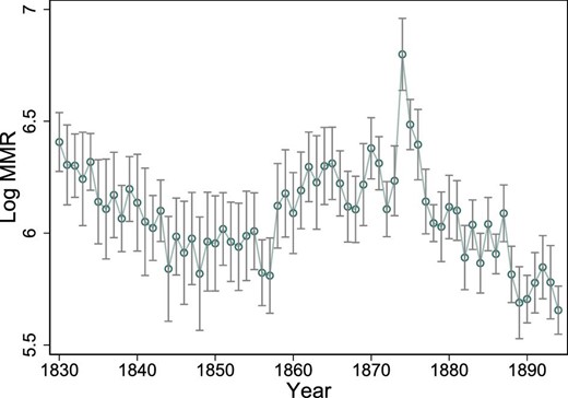
Log MMR. The average of the logarithm of the MMR over time. The vertical lines show the 95% confidence intervals around the yearly averages.
Summary statistics.
| Mean | SD | Min | Max | Observations | |
|---|---|---|---|---|---|
| Maternal deaths | 23.1 | 14.6 | 0.0 | 116.0 | 1,625 |
| MMR | 489 | 285 | 0 | 4,048 | 1,625 |
| Number of female deaths excluding maternal deaths | 1,482 | 645 | 254 | 4,160 | 1,625 |
| Number of midwives | 68.8 | 58.6 | 5.0 | 377.0 | 1,559 |
| Number of midwives per 1000 females | 1.0 | 0.4 | 0.2 | 2.0 | 850 |
| Number of live births | 4,782 | 2,087 | 827 | 10,827 | 1,625 |
| Number of stillbirths | 149 | 72 | 12 | 361 | 1,625 |
| Stillbirth rate | 30.0 | 6.4 | 10.4 | 71.5 | 1,625 |
| Number of infant deathts | 654 | 286 | 60 | 1,576 | 1,625 |
| Harvest yield | 4.0 | 1.2 | 0.0 | 6.0 | 1,625 |
| Number of trained midwives | 3,043 | 2,063 | 263 | 10,820 | 875 |
| Share of midwife-assisted births | 0.56 | 0.25 | 0.03 | 0.98 | 875 |
| Number of female emigrants | 395 | 441 | 0 | 2,185 | 850 |
| Number of community-based doctors | 5.3 | 2.0 | 0.0 | 9.0 | 850 |
| Total number of doctors | 25 | 25 | 4 | 199 | 850 |
| Percentage of mothers aged below 21 | 1.3 | 0.5 | 0.4 | 6.6 | 750 |
| Percentage of mothers aged 21–25 | 14.3 | 2.2 | 6.9 | 21.1 | 1,624 |
| Percentage of mothers aged 26–30 | 25.6 | 2.0 | 13.5 | 34.7 | 1,624 |
| Percentage of mothers aged 31–35 | 26.1 | 1.6 | 16.6 | 31.3 | 1,624 |
| Percentage of mothers aged 36–40 | 20.4 | 1.9 | 13.6 | 28.1 | 1,624 |
| Percentage of mothers aged 41–45 | 10.5 | 1.9 | 4.8 | 23.0 | 1,624 |
| Percentage of mothers aged 46–50 | 1.5 | 0.5 | 0.2 | 3.3 | 1,623 |
Notes: The variables are at the region and year levels. MMR is the number of maternal deaths per 100,000 births. The stillbirth rate is the number of stillbirths per 1,000 births. Harvest yield is a measure of harvest success, where zero is the lowest and six is the highest. Percent of mothers aged below 21 is the percent of mothers giving birth who were younger than 21 years and so on for the other age categories. The variables with fewer observations are only available for the later years (typically 1861–1894). Community-based doctors were called “Provinsialläkare”.
In 1830, the average number of midwives in a region was 40, with a minimum of 5 and a maximum of 205. In 1894, the average number of midwives increased to 103, with a minimum of 43 and a maximum of 346. Figure 2 displays the yearly variation in the logarithm of the number of midwives (i.e., the explanatory variable of interest). Again, the variable is expressed in logarithmic form to make it comparable with the empirical specification in the next section. The average share of midwife-assisted births was 56, with a range of 3%–98%. The share of midwife-assisted births is depicted in Online Appendix Figure A.9. Table 1 displays the summary statistics of the regional data.
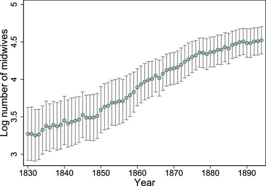
Log number of midwives. The average of the logarithm of the number of midwives over time. The vertical lines show the 95% confidence intervals around the yearly averages.
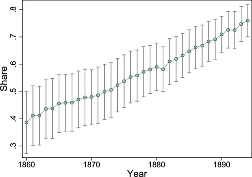
Share of midwife-assisted births. The average share of midwife-assisted births among all births, depicted over time. Data on whether a birth was assisted by a midwife or not are not available before 1860. The vertical lines show the 95% confidence intervals around the yearly averages.
The maternal mortality data were collected at the parish level by the clergy and then compiled annually by the Office of the Registrar General (Tabellverket) (Högberg, Wall, and Broström 1986). More information about the data can be found in Online Appendix C.
3. Empirical Designs and Results
In this section, we define the causal parameters of interest and how they can be estimated with our data.
There are a number of econometric problems that need to be addressed in order to estimate the parameters in these three equations without bias. The first issue is that one cannot estimate any of these parameters directly because the denominator, that is, births, is exactly the same for the dependent and independent variables in all equations. Indeed, Kronmal (1993) shows that this induces a spurious correlation between the two ratios. A solution to this type of ratio problem (e.g., Clemens and Hunt 2019) is to take the logarithm of the equation of interest and include the logarithm of the denominator as a control variable in order to preserve the original interpretation of the population regression model. For this reason, we will always estimate equations (1)–(3) in logarithmic form to avoid the ratio problem.
The second problem is that our measure of midwife availability should be unrelated to the unobserved factors in the error term. In other words, we would ideally like to make use of external (supply) shocks to the availability of midwives that are uncorrelated with the local demand for midwives. Indeed, the general idea of our empirical approach is that we can estimate the relationship between midwife availability and maternal mortality by using institutional features of the supply side of the Swedish health system, that is, the use of supply-side variables to help resolve identification problems on the demand side of the health care market. The first design is based on supply shocks or sharp “discontinuities” in the availability of midwives across time and place as induced by the limited supply at the national level. The second design makes use of the opening of the new midwifery school in the city of Gothenburg in 1856, which dramatically increased the supply of midwives in that part of Sweden.
Estimating the causal effect of these types of supply shocks (i.e., public health intervention) only requires that the intervention is as good as random (e.g., Duflo and Kremer 2003). By contrast, to estimate the causal effect of midwife-assisted births on maternal mortality, an exclusion restriction is also required, namely, that the midwifery policy only affected maternal mortality via midwife-assisted deliveries. In our context, the exclusion restriction seems plausible because there was (i) no referral system in the case of complications during delivery and (ii) a licensed midwife was essentially not allowed to perform any important medical treatments other than deliveries.
In addition, we provide suggestive empirical support that the exclusion restriction is likely to hold because both negative and positive supply shocks to the availability of midwives yield similar impact estimates. Indeed, the exclusion restriction would be violated if a licensed midwife provided “training” on how to safely assist births to a TBA. In such a case, one would expect that a negative supply shock would have less of an impact on MMR than a positive shock if there were such information transfers between licensed midwives and TBAs because then a TBA could also reduce MMR to almost the same extent as a licensed midwife.27,28 Reassuringly, there do not seem to be such information spillover effects.
Below, we describe the two empirical designs in detail.
3.1. Design 1: Supply Shocks of Midwives
The idea of this design is to isolate regional supply shocks (large changes) in the availability of midwives, which are arguably uncorrelated with the demand for midwives. To implement this design, we make use of a difference-in-differences study with region-specific time trends. With this particular design, it is possible to relax both the common trend assumption in a standard difference-in-differences design and the assumption of strict exogeneity of the (midwife) policy because the number of time periods is very large, that is, 65 years.29 Indeed, in a conventional difference-in-differences design, there are typically only a few years before and after a policy change, making it necessary to assume strict exogeneity to be able to deal with unobserved time-invariant cross-sectional heterogeneity. In sharp contrast, the policy is only required to be sequentially exogenous conditional on the unobserved effect (Wooldridge 2010, p. 368) in our design. As a result, our approach is therefore robust to potential feedback effects. For example, if midwives are placed in regions with a high MMR (i.e., those areas that lack trained midwives), we can deal with this feedback problem by including lags of MMR without introducing bias in the fixed-effect approach.30 On the other hand, the standard difference-in-differences design is unable to deal with this type of violation of strict exogeneity.
Clearly, having a large number of time periods (i.e., 65 years) also means that the common trend assumption is unlikely to hold in our setting. Indeed, it is unlikely that all 25 regions would have had similar trends in MMR in the absence of public health interventions. Nonetheless, in a model that includes a region-specific time trend, the identification of the causal effect is based on sharp deviations from otherwise smooth trends, even where trends are not common.31 The identification relies on the appearance and size of a “jump” in the outcome (MMR) at the time of the shock to the availability of midwives. In other words, if the public health intervention does not induce a sharp deviation from the trend in MMR, the identification fails (e.g., if the causal effect on maternal mortality emerges only gradually after a sharp change in midwife availability). Figure 4 nicely illustrates our identification approach for one of the regions (Stockholm).32 Specifically, it shows that there is a sharp increase in midwives in the mid-1870s that is followed by an equally sharp decline in MMR.
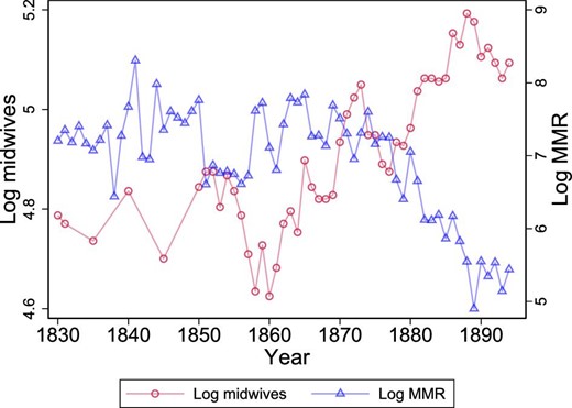
Example region illustrating design 1. The graph shows the log number of midwives and log MMR over time for one of the regions. The graph illustrates the type of variation in midwives that is used to identify the effect of midwives on MMR. All regions are depicted in Online Appendix A.
Starting with the functional form of the region-specific trend f(t), both a linear specification and a quadratic specification are used (see Table 3 for the results). In effect, f(t) controls for smooth changes in the outcome, while the explanatory variable—log (midwivesgt)—captures any discontinuous effects on the availability of midwives. Consequently, there must be sharp changes or discontinuities in the availability of midwives at the regional level to be able to estimate the parameter β.
Regarding the specification of the dynamic response of MMR to a change in the supply of midwives, it seems that any change in the local demand for midwife-assisted births is likely to be much smoother than any sharp change in the regional availability of midwives. A distributed lag specification, that is, including lags of log(midwivesgt), can be used to probe the timing issue (see Online Appendix Table B.3 for the result). Ideally, the causal effect should appear immediately with little or no dynamic effects; otherwise, the supply shocks may be correlated with slow-moving changes in the demand for midwife-assisted births.
Naturally, there are both large positive and negative shocks to the availability of midwives at the regional level because the capacity to train and license midwives was severely limited, as discussed above.34 Clearly, as long as these large regional supply shocks are uncorrelated with the local demand for midwives, both types of variations are permissible ways to identify the effect β.
Moreover, the interpretation that midwife availability affects MMR through midwife-assisted births and not through general health information would also be strengthened if the results are similar for both sharp positive and negative changes in the availability of midwives (see Online Appendix Table B.4 for the result). If instead midwife availability affects MMR through dissemination of general health information, a positive effect is likely to be sustained even after a subsequent decrease in midwife availability, and the magnitude of a negative shock would be smaller.
Equation (4) is a grouped data regression or (pseudo)-panel data at the regional level, which may be prone to measurement error problems. However, there are few or no measurement errors in these regional averages because the data cover the universe of births and the average number of yearly births within a region is large,35 almost 5,000 (see Table 1).36 More importantly, there is little or no measurement error in the key regressor of interest, that is, the number of regional midwives, which does not vary at the individual level but only at the group level,37 that is, the region–year level. As a result, a bias in the estimated effect due to measurement error problems is likely to be negligible because the measurement error problem is only in the dependent variable and because the measurement errors are most likely of the classic form.
There is also the question of whether one should estimate the grouped data regression (4) by weighted least-squares (WLS; weighted by size of the regional birth cohort) to return to the micro data relationship, that is, the underlying micro data set with nearly 8 million births during the period of 1830–1894. However, this is an open question because an argument can be made that an unweighted analysis of aggregates is to be preferred (Angrist and Pischke 2009). Nonetheless, Solon, Haider, and Wooldridge (2015) recommend reporting both the weighted and unweighted estimates because the contrasts between ordinary least-squares (OLS) and WLS estimates can be used as a diagnostic for model specification or endogenous sampling (see Table 3 and Online Appendix Table B.1 for the results).38
Another specification issue concerns the fact that midwives were likely to be placed in regions with already high maternal mortality (e.g., due to the absence of midwives). One way of dealing with this issue of feedback from MMR to future values of midwife availability is to include a lagged dependent variable, log (MMRgt −1), in equation (4). However, this introduces a bias in a panel data model with fixed effects (Nickell 1981).39 Nonetheless, the asymptotic bias of the fixed-effect estimator is of the order of T. Thus, because the number of years is very large, T = 65, the bias is likely to be minimal (see Online Appendix Table B.2 for the result).40
As a final comment concerning regression (4), the standard errors are clustered at the regional level to address problems with serial correlations in the errors within clusters. Importantly, Hansen (2007) has shown that the clustered standard errors work well even if the number of clusters, N, is fairly small as long as the number of time periods, T, is sufficiently large, which is the case because T = 65 and N = 25.41
Table 2 displays the results of this test, showing that none of the 19 estimates is significantly different from zero at the 5% level. Moreover, most of the estimates in Table 2 are also small and of different signs. Thus, these results provide strong support that the sharp changes in the availability of midwives can be considered as good as random and therefore not related to the demand for midwives. It is particularly noteworthy that fertility (a demand-side variable), infant mortality (a measure of economic development and population health), and female mortality (a measure of population health) are not associated with the sharp changes in the availability of midwives. This result is also in line with Loudon’s finding that maternal mortality, in contrast to other death rates such as infant mortality, has been insensitive to social and economic conditions (Loudon 1987).
Test of conditional randomization.
| (1) | (2) | (3) | (4) | (5) | (6) | (7) | |
|---|---|---|---|---|---|---|---|
| Panel A: time-varying confounding factors | |||||||
| log | log | log | log | log | |||
| (births) | (female death) | (infant death) | (doctors) | (emigrants) | |||
| log(midwives) | −0.04 | 0.02 | −0.04 | 0.04 | −0.01 | ||
| (0.04) | (0.04) | (0.03) | (0.06) | (0.31) | |||
| Panel B: age distribution of mothers giving birth | |||||||
| ≤20 | 21–25 | 26–30 | 31–35 | 36–40 | 41–45 | 46–50 | |
| log(midwives) | −0.00* | −0.00 | 0.00 | −0.00* | 0.00 | 0.00 | 0.00 |
| (0.00) | (0.00) | (0.00) | (0.00) | (0.00) | (0.00) | (0.00) | |
| Panel C: indicators of harvest yield: 0–6 | |||||||
| H = 1 | H = 2 | H = 3 | H = 3 | H = 4 | H = 5 | H = 6 | |
| log(midwives) | 0.01 | 0.03 | 0.02 | 0.05 | −0.03 | −0.01 | −0.06 |
| (0.03) | (0.02) | (0.03) | (0.08) | (0.08) | (0.06) | (0.06) | |
Notes: Each entry is a separate regression with each covariate (denoted in the column heading) as the dependent variable. All specifications include a full set of region- and time-fixed effects together with region-specific time trends, and the covariate log(births) [except in the regression with log(birth) as the dependent variable]. log(·) denotes the logarithm of the variable within parentheses. The dependent variables in panel A are log number of births per region and year, log number of female deaths excluding maternal deaths, log number of infant deaths, log number of total doctors, and log number of female emigrants. The dependent variables in panel B are the percent of mothers giving births within each age category. The dependent variables in panel C are harvest indicators, where Harvest = 0 is harvest failure and Harvest = 6 is the most successful harvest. Standard errors, clustered at the regional level, are within parentheses. Coefficients significantly different from zero are denoted by the following system: *10%, **5%, and ***1%.
Table 3 displays the results for the reduced-form relationship between MMR and midwives, that is, specification (4). All specifications in Table 3 are unweighted OLS regressions. The estimate in column (1), without any controls for additional confounders, is −0.19 and statistically significant at the 5% level. The 95% confidence interval is [−0.36, −0.03]. Because both the dependent and independent variables are expressed in logarithmic form, the interpretation of the estimated coefficient is that a doubling of the number of midwives leads to a 19% reduction in MMR. Adding the additional confounders has little or no impact on the estimated effect, as seen in columns (2)–(6). This result is also what should be expected from the previous finding, that is, that these sets of confounders are not related to the midwifery policy conditional on region-fixed effects, time-specific effects, and region-specific time trends. Importantly, the estimated effect is not affected if a quadratic region-specific time trend is added in column (7), which again suggests that our identification approach is credible.
Estimate design 1: the effect of (log) midwife availability on (log) MMR (unweighted estimates).
| (1) | (2) | (3) | (4) | (5) | (6) | (7) | |
|---|---|---|---|---|---|---|---|
| log(midwives) | −0.19** | −0.21** | −0.20** | −0.19** | −0.19** | −0.19** | −0.21** |
| (0.08) | (0.08) | (0.07) | (0.07) | (0.07) | (0.07) | (0.07) | |
| log(births) | Yes | Yes | Yes | Yes | Yes | Yes | |
| log(infant death) | Yes | Yes | Yes | Yes | Yes | ||
| log(female death) | Yes | Yes | Yes | Yes | |||
| Age | Yes | Yes | Yes | ||||
| Harvest | Yes | Yes | |||||
| Regional time trends | Linear | Linear | Linear | Linear | Linear | Linear | Quadratic |
| Observations | 1,608 | 1,608 | 1,608 | 1,608 | 1,606 | 1,606 | 1,606 |
Notes: Each column is a separate regression. All specifications include a full set of region- and time-fixed effects together with region-specific time trends. The dependent variable is log(MMR), where MMR is the maternal mortality ratio. log(·) denotes the logarithm. Age refers to the age distribution of mothers giving birth (see Table 1). Standard errors, clustered at the regional level, are in parentheses. The regressions are based on data from the years 1830–1894. The within (overall) R2 ranges from 0.36 (0.49) in column (1) to 0.41 (0.53) in column (7). Coefficients significantly different from zero are denoted by the following system: *10%, **5%, and ***1%.
Online Appendix Table B.1 presents exactly the same specifications as in Table 3, with regressions weighted by the size of the regional birth cohort. The results from WLS are almost identical to the unweighted estimates in Table 3. Thus, reassuringly, weighting does not matter for the results of the effect of midwives on MMR.
Another specification check is to control for a lagged dependent variable because one could argue that the midwifery policy followed a strategy of placing midwives in regions with a previously high MMR. Online Appendix Table B.2 presents these results for both the OLS (columns (1)–(3)) and WLS specifications (columns (4)–(6)). For ease of comparison, columns (1) and (4) restate the results from the specifications without lagged MMR, as displayed in Table 3 and Online Appendix Table B.1. The estimated effect is only slightly affected by adding lagged outcomes. The estimate of the first-order lag is also rather small (0.08–0.09), while the second is very close to zero and not significantly different from zero. These small estimates imply that the lagged MMR has only limited predictive content for future MMR, which is also consistent with the findings in the medical literature that most obstetric complications occur around the time of delivery and cannot be predicted.43
The effect of changes in midwife availability may not only affect maternal mortality in the current period but also feed into future periods.44 However, an additional specification check is to estimate a distributed lag model, that is, lags of log(midwives), to investigate timing issues of the causal effect. Online Appendix Table B.3 shows the results for a one- and two-lag specification for both unweighted and weighted regressions. Importantly, there are no dynamic causal effects because the coefficients on both the first and second lag of log(midwives) are close to zero and not significantly different from zero. Thus, the effect of midwives on MMR seems to occur immediately.
A final check is to test whether the results are similar for both positive and negative changes in the availability of midwives. We create dummy variables for observations with positive, negative, and zero changes in midwife availability. Columns (1) and (2) in Online Appendix Table B.4 display the results with an interaction term of positive changes in midwife availability and midwife availability, and columns (3) and (4) present the results for negative changes. The interaction term is not statistically significant and is close to zero in both specifications. Both types of variation also yield similar impact estimates of midwife availability.
In summary, all specification tests suggest that the empirical strategy, that is, a difference-in-differences design with region-specific time trends, is compelling.
Having estimated the intent-to-treat effect, we next turn to the estimate of the relationship between MMR and midwife-assisted births. This estimate requires that we can measure the take-up of the midwifery policy, that is, the share of midwife-assisted births. Birth assistance was only recorded for part of the investigated period, namely, the years 1861–1894. Thus, we can only estimate take-up for this shorter period. Table 4 displays the results: Panel A shows the estimates of the take-up of the midwifery policy, panel B shows the estimates of the intent-to-treat effect (or the reduced-form effect), and panel C shows the treatment effect, that is, the relationship between MMR and the share of midwife-assisted births, where the midwifery policy is used as the instrumental variable. We use the same specification as previously (i.e., region-fixed effects, time-specific effects, and region-specific time trends) with the extension that we can now also control for two additional confounders that are available from 1860: the number of female emigrants and the number of doctors, where both variables are expressed in logarithmic form. We also show results where we control for the lagged MMR.
Estimate design 1, years 1861–1894.
| (1) | (2) | (3) | (4) | (5) | (6) | (7) | (8) | (9) | (10) | (11) | |
|---|---|---|---|---|---|---|---|---|---|---|---|
| Panel A: the relationship between midwife-assisted births and midwife availability | |||||||||||
| First-stage | 0.19*** | 0.19*** | 0.19*** | 0.19*** | 0.19*** | 0.19*** | 0.19*** | 0.19*** | 0.19*** | 0.18*** | 0.19*** |
| (0.05) | (0.05) | (0.05) | (0.05) | (0.05) | (0.05) | (0.05) | (0.05) | (0.05) | (0.05) | (0.05) | |
| Panel B: the relationship between MMR and midwife availability | |||||||||||
| Reduced form | −0.38*** | −0.38*** | −0.39*** | −0.40*** | −0.39*** | −0.36*** | −0.37*** | −0.37*** | −0.34*** | −0.38*** | −0.35*** |
| (0.13) | (0.13) | (0.13) | (0.13) | (0.12) | (0.12) | (0.12) | (0.12) | (0.11) | (0.11) | (0.11) | |
| Panel C: the relationship between MMR and midwife-assisted births | |||||||||||
| Instrumental variable estimate | −1.97** | −2.03** | −2.09** | −2.10** | −2.09** | −1.93** | −1.99** | −1.98** | −1.77** | −2.08** | −1.81** |
| (0.89) | (0.90) | (0.92) | (0.92) | (0.87) | (0.85) | (0.86) | (0.86) | (0.76) | (0.87) | (0.77) | |
| log(births) | Yes | Yes | Yes | Yes | Yes | Yes | Yes | Yes | Yes | Yes | |
| log(infant death) | Yes | Yes | Yes | Yes | Yes | Yes | Yes | Yes | Yes | ||
| log(female death) | Yes | Yes | Yes | Yes | Yes | Yes | Yes | Yes | |||
| Age | Yes | Yes | Yes | Yes | Yes | Yes | Yes | ||||
| Harvest | Yes | Yes | Yes | Yes | Yes | Yes | |||||
| log(emigrants) | Yes | Yes | Yes | Yes | Yes | ||||||
| log(doctors) | Yes | Yes | Yes | Yes | |||||||
| Lagged MMR | Yes | Yes | Yes | ||||||||
| Weighted | Yes | Yes | |||||||||
| First stage F | 14 | 15 | 15 | 14 | 15 | 15 | 15 | 14 | 14 | 14 | 13 |
| Observations | 848 | 848 | 848 | 848 | 848 | 848 | 842 | 842 | 842 | 840 | 840 |
Notes: Each column is a separate regression. All specifications include a full set of region- and time-fixed effects together with region-specific time trends. The dependent variable is log(MMR), where MMR is the maternal mortality ratio. log(·) denotes the logarithm. Age refers to the age distribution of mothers giving birth (see Table 1). The estimates are weighted by the size of the yearly regional birth cohort. Standard errors, clustered at the regional level, are within parentheses. The regressions are based on data from the years 1861–1894 because data on whether a birth was assisted by a midwife or not are not available before 1860. Coefficients significantly different from zero are denoted by the following system: *10%, **5%, and ***1%.
Panel A (Table 4) shows that a doubling of midwives leads to a 19% increase in the take-up of midwife-assisted births. The 95% confidence interval is [0.09, 0.30]. This estimate is strikingly robust because it is completely insensitive to adding the confounding factors (columns (2)–(8)), weighting by the number of births (columns (9) and (11)) or controlling for the lagged MMR (columns (10) and (11)). It is also noteworthy that the estimate of the lagged MMR is close to zero,45 which again suggests that it is very hard to predict future MMR based on previous MMR. Moreover, the cluster-robust first-stage F-statistic is in the range of 13–15 in all specifications, suggesting that this instrument is not weak (Staiger and Stock 1997).46 Panel B (Table 4) displays that the estimates of the intent-to-treat effect (or the reduced-form effect) are in the range of −0.34 to −0.40, meaning that a doubling of midwives leads to a 34%–40% reduction in MMR. The 95% confidence intervals range at most from −0.66 to −0.11. Once more, the estimated effect is insensitive to adding confounding factors, weighting, and controlling for the lagged MMR. It is also noteworthy that the estimated effect is larger than the corresponding estimates in Table 3 and Online Appendix Table B.1, using data for the entire period of 1830–1894. That the estimated policy effect is larger in the later period is not surprising, however, because these midwives had more extensive training, as previously noted.
Next, we turn to the results from estimating the effect of midwife-assisted births on MMR. Here, as previously discussed, we use midwifery policy as an instrumental variable for the share of midwife-assisted births. Panel C (Table 4) shows that the effect, that is, the elasticity, is approximately −2, that is, a 1% increase in the share of midwife-assisted homebirths reduced maternal mortality by approximately 2%. The 95% confidence interval ranges from −3.91 to −0.24. The regression is based on data from 1861 to 1894, because data on midwife-assisted births are available only after 1860.
3.2. Design 2: The New Midwifery School
In this design, we explicitly exploit the opening of a new midwifery school in the city of Gothenburg in southwest Sweden in 1856 (see the map in Online Appendix Figure A.14). This design nicely complements the previous strategy that used data after 1860 because both designs make use of a variation in the availability of midwives after 1860. In other words, one would expect these two designs to produce similar results about the effect of midwife availability on MMR. With this design (using the new midwifery school), we can only estimate the policy effect—parameter β in equation (1)—and not the causal effect of midwife-assisted births on MMR. This is because the take-up of the midwife policy (whether a birth was assisted by a midwife) is only recorded from 1861, that is, after the opening of the midwifery school in 1856.
The opening of a new midwifery school drastically increased the number of examined midwives in regions close to Gothenburg.47 This is clearly supported by Figure 5, which shows the log number of midwives separately by regions treated and not treated by the opening of the midwifery school.
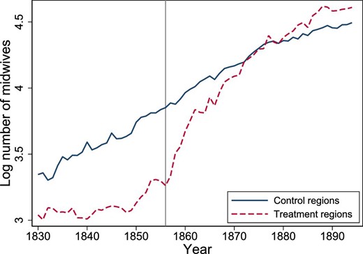
Log number of midwives by treatment group. The mean value of the logarithm of the number of midwives, by treatment group and year. Design 2, years 1830–1894. The gray vertical line shows the opening of the new midwifery school in 1856. The treatment group consists of the six regions: Göteborg, Älvsborg, Halland, Jönköping, Skaraborg, and Värmland. The control groups are all other regions.
For the control group, that is, regions farthest away from the new midwifery school, to be a valid comparison group for the treatment group, that is, regions where midwife availability was affected by the new school, midwife availability and maternal mortality should have evolved similarly absent the opening of the new midwifery school. Hence, the decision of where to locate the new midwifery school should not have been based on potential future trends in midwife availability and maternal mortality, because the parallel trend assumption would then be violated. We have not found any evidence that the Swedish authorities took these issues into consideration when deciding where to locate the new midwifery school.
Table 5 reports the results from design 2. In panel A, we report estimates of the first-stage effect, that is, parameter σ in equation (7). In panel B, we report the estimates of the reduced-form effect, that is, parameter ρ in equation (6), and in panel C, we report the policy effect, the reduced-form effect scaled by the first-stage effect, using an instrumental variable approach. We control for the same set of confounders as those used in the previous approach. Thus, we control for the exact number of births in column (2), column (3) includes infant deaths, column (4) controls for all other female deaths except maternal deaths, column (5) includes the age distribution of mothers, while column (6) controls for a full set of indicators of harvest yield. Column (7) weights the estimates by the number of births in each region and year.
Estimate design 2, years 1830–1894.
| (1) | (2) | (3) | (4) | (5) | (6) | (7) | |
|---|---|---|---|---|---|---|---|
| Panel A: the relationship between midwife availability and the school opening | |||||||
| Midwife availability | 0.44*** | 0.47*** | 0.47*** | 0.48*** | 0.43*** | 0.43*** | 0.42*** |
| (0.13) | (0.13) | (0.13) | (0.14) | (0.14) | (0.14) | (0.14) | |
| Panel B: the relationship between MMR and the school opening | |||||||
| Reduced form | −0.13** | −0.15** | −0.14** | −0.14** | −0.14** | −0.13** | −0.09 |
| (0.06) | (0.06) | (0.06) | (0.06) | (0.06) | (0.06) | (0.06) | |
| Panel C: the relationship between MMR and midwife availability | |||||||
| Instrumental variable estimate | −0.30* | −0.32* | −0.30* | −0.29* | −0.31* | −0.30* | −0.21 |
| (0.18) | (0.17) | (0.15) | (0.15) | (0.18) | (0.18) | (0.18) | |
| log(births) | Yes | Yes | Yes | Yes | Yes | Yes | |
| log(infant death) | Yes | Yes | Yes | Yes | Yes | ||
| log(female death) | Yes | Yes | Yes | Yes | |||
| Age | Yes | Yes | Yes | ||||
| Harvest | Yes | Yes | |||||
| Weighted | Yes | ||||||
| First stage F | 11 | 12 | 12 | 12 | 10 | 10 | 8 |
| Observations | 1,610 | 1,610 | 1,610 | 1,610 | 1,608 | 1,608 | 1,608 |
Notes: Each entry is from separate regressions. All specifications include a full set of region- and time-fixed effects. The dependent variable in panel A is the number of midwives in logarithmic form. The dependent variable in panel B and panel C is the MMR in logarithmic form. Panel C is the Wald estimator, the ratio between the reduced-form estimate and the first-stage estimate. log(·) denotes the logarithm. Age refers to the age distribution of mothers giving birth (see Table 1). The weighted estimates are weighted by the size of the yearly regional birth cohort. Standard errors, clustered at the regional level, are within parentheses. The within (overall) R2 ranges from 0.76 (0.91) to 0.79 (0.92) in panel A, from 0.28 (0.43) to 0.31 (0.45) in panel B, and from (0.39) to (0.41) in panel C. Coefficients significantly different from zero are denoted by the following system: *10%, **5%, and ***1%.
Panel A (Table 5) shows that the first-stage estimate is in the range of 0.43–0.48, which implies that the treatment group—the regions closest to the new midwifery school in Gothenburg—increased its number of midwives by 55%–62% compared to the control group.48 Figure 5 clearly illustrates this result because it shows that the treatment group had far fewer midwives than the control group before the opening of the midwifery school in 1856, followed by a very sharp increase in the availability of midwives such that the two groups had the same number in 1872. The estimated first-stage effect is also statistically significant because the cluster-robust F-statistic is between 8 and 12.
Panel B (Table 5) displays that the reduced-form estimate (the effect of the new midwifery school on MMR) is between −0.09 and −0.15 and is statistically significant at the 5% level in all specifications except one. Thus, this finding suggests that the opening of the midwifery school reduced the MMR by 9%–15% in the treatment areas compared to the control areas.49 Figure 6 provides additional support for this finding because the treatment areas had consistently higher MMR than the control regions before the opening of the midwifery school in 1856 and because this difference in MMR between the treatment and control areas largely disappeared shortly after 1856.
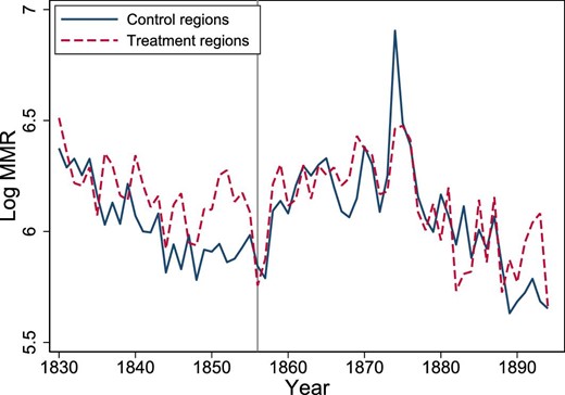
Log MMR by treatment group. The mean value of the logarithm of MMR by treatment group and year. Design 2, years 1830–1894. The gray vertical line shows the opening of the new midwifery school in 1856. Log MMR is the logarithm of the maternal mortality ratio. The treatment group are the six regions Göteborg, Älvsborg, Halland, Jönköping, Skaraborg, and Värmland. The control group consists of all other regions.
Panel C (Table 5) shows the estimate of the midwife policy effect using an instrumental variable approach where the policy effect is the ratio of the reduced-form effect and the first-stage effect. The policy effect is approximately −0.30, that is, a doubling of midwives leads to a 30% reduction in MMR. The size of this estimate is in the same ballpark as those in panel B of Table 4. In other words, this finding bolsters both internal and external validity because we obtain similar results from the two different research designs.
To further probe the identifying assumption in the difference-in-differences design, we test whether the treatment and control groups have parallel trends in their outcomes before the intervention, that is, the opening of the midwifery school in 1856. To conduct such a test, we create the following eight indicator variables for treatment before 1856: |$1[\rm {treatment\,\, group} \times \rm {year}=1855]$|, |$1[\rm {treatment\,\, group} \times \rm {year}=1854],\ldots , 1[\rm {treatment\,\, group} \times \rm {year}=1848]$|. With these eight indicator variables, we can test whether there is an effect of the treatment up to eight years before the actual treatment in 1856. Table 6 reports the results of adding all these indicators to the difference-in-differences specifications reported in the last column of Table 5. Column (1) in Table 6 shows the estimates from the first-stage specification post- and pretreatment. The estimate in the first row is the impact effect, which is 0.40. This estimate thus differs little from the corresponding estimates in panel A of Table 5. In addition, all other eight “placebo” estimates (pretreatment) are much smaller, and all are also negative. This clear change in the sign of the estimated effects strongly suggests that there is a “structural break” in the first-stage relationship after 1855. The treatment group and year interactions are also depicted in Online Appendix Figure A.10.
Test of parallel trends, design 2.
| First-stage | Reduced form | |
|---|---|---|
| Post-treatment | ||
| 1 [treatment group = 1 and year > 1855] | 0.40** | −0.10* |
| (0.15) | (0.06) | |
| Pre-treatment | ||
| 1 [treatment group = 1 and year = 1855] | −0.10 | −0.05 |
| (0.12) | (0.17) | |
| 1 [treatment group = 1 and year = 1854] | −0.10 | 0.09 |
| (0.11) | (0.14) | |
| 1 [treatment group = 1 and year = 1853] | −0.06 | 0.11 |
| (0.13) | (0.15) | |
| 1 [treatment group = 1 and year = 1852] | −0.11 | 0.26 |
| (0.13) | (0.16) | |
| 1 [treatment group = 1 and year = 1851] | −0.15 | 0.15 |
| (0.10) | (0.15) | |
| 1 [treatment group = 1 and year = 1850] | −0.15 | 0.05 |
| (0.09) | (0.12) | |
| 1 [treatment group = 1 and year = 1849] | −0.15* | 0.10 |
| (0.08) | (0.21) | |
| 1 [treatment group = 1 and year = 1848] | −0.10* | 0.06 |
| (0.06) | (0.18) | |
| Observations | 1,606 | 1,606 |
Notes: Each column is a separate regression. All specifications include a full set of region- and time-fixed effects and a full set of control variables, that is, log(births), log(infant deaths), log(female deaths), age distribution, and harvest indicators. The dependent variable in the first-stage regression is the number of midwives in logarithmic form. The dependent variable in the reduced-form regression is the logarithm of the MMR. The treatment group are the six regions: Göteborg, Älvsborg, Halland, Jönköping, Skaraborg, and Värmland. The control group consists of all other regions. The within (overall) R2 is 0.79 (0.92) for the first stage and 0.31 (0.45) for the reduced form. Coefficients significantly different from zero are denoted by the following system: *10%, **5%, and ***1%.
Turning to the reduced-form relationship in column (2) of Table 6, the same type of switch in the sign of the estimated effect can be noticed. While the estimated effect is −0.10, all eight placebo effects except one are positive. These clear patterns in the signs of the placebo effects suggest that the treatment and control groups had diverging trends in the number of midwives and MMR before 1856 and converging trends thereafter.50 This finding is also consistent with graphical evidence from Figures 5 and 6. Figure 5 shows the first-stage relationships for the treatment and control groups, while Figure 6 displays the reduced-form relationship. In other words, the treatment group has, on average, a much larger MMR than the control group before 1856, but this difference in MMR disappears immediately after 1856 because both groups then have similar levels and trends in MMR. The treatment and year interactions are also depicted in Online Appendix Figure A.11.
4. Midwives, Stillbirths, and Infant Mortality
In this short section, we analyze the effect of midwives on stillbirths and infant mortality. As noted above, it has been argued that perinatal mortality may be used as a proxy for maternal mortality (Campbell, Koblinsky, and Taylor 1995). Because perinatal mortality is defined as stillbirths plus early neonatal deaths at less than 7 days of age, we can essentially use stillbirths as a measure of perinatal mortality. Panel A of Table 7 shows the reduced-form relationship using the same two empirical strategies as before but using the logarithm of the stillbirth rate as the dependent variable instead of MMR. Columns (1) and (2) show the results from the first design (supply shocks in midwife availability), while column (3) displays the results from the second design (opening of a midwifery school). There is no evidence that the availability of midwives is related to stillbirths because none of the three estimates is significantly different from zero. In addition, even the signs differ across the specifications. Thus, the conclusion is that stillbirths cannot be used as a proxy for maternal mortality. In other words, to estimate whether a public health intervention had an impact on maternal mortality, one must have data on MMR. Similarly, we find that midwives had no effect on infant mortality, as shown in panel B of Table 7.
Estimates of stillbirth and infant mortality on log midwives.
| Design 1 | Design 1 | Design 2 | |
|---|---|---|---|
| 1830–1894 | 1861–1894 | 1830–1894 | |
| (1) | (2) | (3) | |
| Panel A: log(stillbirth rate) | |||
| −0.03 | −0.05 | 0.04 | |
| 0.02 | 0.05 | 0.03 | |
| Panel B: log(infant deaths) | |||
| −0.04 | −0.03 | 0.01 | |
| 0.02 | 0.04 | 0.03 | |
| Control variables | Yes | Yes | Yes |
| Observations | 1,608 | 850 | 1,623 |
Notes: Each entry is a separate regression. All specifications include a full set of region- and time-fixed effects together with region-specific time trends. The control variables log(births), log(infant deaths), log(female deaths), age distribution, and harvest indicators are included in panel A. In panel B, all covariates except log(infant) are included. log(·) denotes the logarithm. Stillbirth rate is the number of stillbirths per 1,000 births. Infant deaths is the number of infant deaths. Standard errors, clustered at the regional level, are within parentheses. The within (overall) R2 ranges from 0.47 (0.72) to 0.33 (0.67) in panel A and from 0.83 (0.97) to 0.80 (0.96) in panel B. Coefficients significantly different from zero are denoted by the following system: *10%, **5%, and ***1%.
5. Discussion and Conclusions
In this paper, we estimated the effect of a public health intervention in the 19th century—home-based intrapartum care by midwives—on MMR, infant mortality, and stillbirth. We find a large effect on MMR but no effects on infant mortality and stillbirths. We argue that the finding that midwives with only 6–12 months of formal training had a large impact on reducing MMR in 19th-century Sweden has potentially important implications as it may be a very effective health strategy to reduce the currently high MMR in low-resource settings. Specifically, the results from this study suggest that having a skilled attendant at home can be a good strategy in low-resource settings because home births may increase the coverage of skilled attendance in rural areas and respond to women’s demand for home-based care.
Acknowledgments
We thank Christina Romlid for sharing her data on midwives. We thank Andreas Madestam and seminar participants at workshops at IFAU, IZA, IIES, University of Stavanger, Sciences Po, Stockholm University, Pompeu Fabra, Lund University, and University of Oslo for useful comments. We thank Handelsbanken's Research Foundations for financial support.
Notes
The editor in charge of this paper was Paola Giuliano.
Footnotes
In many sub-Saharan countries, the lifetime risk of maternal death could be as high as 1 out of 20.
Jokhio, Winter, and Cheng (2005) conduct a clustered RCT consisting of the training of traditional birth attendants (TBAs) in Pakistan. However, despite the fact that there were approximately 10,000 births in both the treatment and control groups, this RCT had very low power to detect any effects on maternal mortality due to the small number of maternal deaths in both the treatment (27 deaths) and control groups (34 deaths). This study clearly illustrates the problem of sample size.
Attaran (2005) also argues “that many of the most important MDGs, including those to reduce…maternal mortality…suffer from a worrying lack of scientifically valid data.” Thus, he concludes that “one cannot know if true progress towards these very important goals is occurring.”
See Sanson-Fisher et al. (2007) for a discussion of why it may be more attractive to use an observational study design rather than an experimental design when evaluating a population-based health intervention.
An exception is Fauveau et al. (1991), who analyze a maternity care program in Matlab, Bangladesh. They find evidence that maternal mortality ratio (MMR) was lower in the intervention area than in the control area. However, this result is questioned by Ronsmans et al. (1997), who argue that the control area is not comparable to the treatment area.
Loudon (1992, p. 414) writes “it is extremely difficult to find statistical evidence that trained midwives lowered the MMR of any country or any region in the nineteenth century.”
We collected these data on our own from the Swedish National Archives and other sources. See the Online Appendix for further information.
See Högberg and Wall (1986) and the references therein for a discussion of Swedish historical vital statistics.
Worldwide, approximately one-third of births take place without the assistance of skilled health personnel. However, only approximately one out of two births in sub-Saharan Africa and South Asia is attended by a skilled provider.
Maternal deaths per 100,000 births.
Interestingly, our estimated effect is similar in magnitude to those produced from a modeling approach by Homer et al. (2014). They show that scaling up midwifery could help reduce maternal mortality, even in resource-constrained environments. For example, a recurrent 5-year increase of 10% coverage of the interventions delivered by midwives would lead to a 27% drop in maternal mortality.
In 2006, The Lancet had a series of papers on the best way to reduce the burden of maternal mortality in developing countries. Four types of health strategies were discussed: (i) health center intrapartum care, (ii) skilled attendance at home, (iii) community health workers at home, and (iv) relatives or traditional birth attendance at home. The recommendation was to use the health center intrapartum care strategy because skilled attendance at home was not considered a viable option.
Loudon (1992) also finds little or no relationship between maternal mortality and infant mortality in the historical data and therefore concludes “it is clear that measures designed to reduce maternal and infant mortality required quite different approaches.”
Högberg, Wall, and Broström (1986) and Högberg (2004) also analyze the relationship between MMRs and midwife-assisted births using historical Swedish data. However, they only compute the preventable fractions of maternal deaths for a small area and without controlling for any confounders. As a result, this type of epidemiological approach cannot convincingly identify any causal relationships. These studies have also been criticized on other grounds. One issue concerns the fact that they exclude from the measure of MMR maternal deaths due to puerperal fever, which is a serious problem according to Loudon (1992). In sharp contrast, this study uses a credible identification strategy and includes all maternal deaths.
Live births per 1,000 people per year.
Maternal death is the death of a woman while pregnant or within 42 days of termination of pregnancy, irrespective of the duration and site of the pregnancy, from any cause related to or aggravated by the pregnancy or its management but not from accidental or incidental causes (WHO 2019).
For the period after 1860, infections are reported to account for nearly 50% of all maternal deaths. However, it is very difficult to know how many of the cases were only due to infections and not a consequence of any of the other direct causes of maternal deaths such as obstructed labor, as there is a considerable overlap among the causes, as noted above. Högberg, Wall, and Broström (1986) argue that the diagnosis of puerperal fever was likely not confounded by septic abortions during the 19th century.
The regions of Malmöhus län och Kristianstad län had their own midwifery school in Lund. On average, fewer than 10 midwives graduated annually from the school in Lund during the 19th century.
It was not until 1842 that Sweden introduced compulsory basic education, but it took a long time to implement. Moreover, there were no requirements for the minimum formal years of schooling, which implied that many children still received little or no education even after 1842.
Number of infant deaths per 1,000 live births.
There is a spike in MMR around the year 1874, a pattern noted in several countries and discussed by Loudon (1992). Loudon (1992) argues that the sharp increase in MMR is due to changes in the virulence of the Streptococcus bacteria. At the same time (1873–1874), there was an outbreak of smallpox in Sweden (Nelson and Rogers 1992).
There are a total of two observations, out of 1,625, where MMR is zero.
If the effect of midwife availability on MMR goes largely through channels other than midwife-assisted births, for example, through information, the effect is likely more persistent, with smaller effects from negative shocks.
More technically, the estimated effect comes from compliers, that is, those who are more likely to have a midwife-assisted birth when the availability of midwives is higher. Defiers, who are less likely to have a midwife-assisted birth with higher availability and more likely to have a midwife-assisted birth with lower availability, seem very unlikely.
The fixed-effect estimator is consistent if T → ∞.
This particular empirical strategy is essentially a type of a regression discontinuity design with time as the forcing variable, as noted by Lee and Solon (2011).
Figures for the other 24 regions are found in Online Appendix A: Figures A.5–A.7.
This is similar to the type of identification strategy used by Miller (2008). The only difference is that his treatment is binary (the introduction of female suffrage laws), while the treatment here is multi-valued (number of midwives).
The overall trend is an increase in the number of midwives (see Figure 2). However, in some years, in some regions, there is a decrease in the number of midwives due to, for example, midwives leaving their positions without being replaced.
Even if one has data from the entire population, the standard errors can be justified using a generalization of randomization inference (Abadie et al. 2014) if taking the perspective that the regression function is intended to capture causal effects.
Devereux (2007) argues that group sizes, that is, the number of annual regional births, should be larger than 2,000 to avoid the problem with measurement errors in pseudo panels.
Since the regressor only varies at the group level, then equation (4) weighted by the group size is identical to OLS on the micro data.
Under exogenous sampling and correct specification of the conditional mean, both OLS and WLS are consistent estimators for the regression coefficients.
Alternatively, if one interprets equation (4) as representing a pseudo-panel regression rather than a true panel data equation, it is possible to control for a lagged dependent variable without introducing bias, as discussed by Wooldridge (2009). In other words, pseudo-panel data make it possible to work with a model that includes both lagged dependent variables and unobserved group fixed effects.
See Wooldridge (2010, p. 302).
Clustering on both region and time, that is, two-way clustering, does not affect the results.
See also the discussion in Pei et al. (2019) about the different ways of testing the identifying assumption. They write, “The confounder can be added as a control variable on the right-hand side of the regression. The identifying assumption is confirmed if the estimated causal effect of interest is insensitive to this variable addition. Alternatively, the candidate confounder can be placed on the left-hand side of the regression instead of the outcome variable. A zero coefficient on the causal variable of interest confirms the identifying assumption. This is analogous to the balancing test typically carried out using baseline characteristics or pre-treatment outcomes in a randomized trial.”
Dividing the midwife coefficient (−0.19) by 1 minus the lagged MMR coefficient (0.09) gives a value of −0.21, where the lagged MMR coefficient is from column (2) in Online Appendix Table B.2.
For example, the estimate in column (10) is −0.04 with a standard error of 0.04.
Olea and Pfueger (2013) argue that one should adjust the critical value in the case of heteroscedasticity, serial correlation and/or clustering. However, this approach would lead to a much more conservative approach in testing for a problem with weak instruments because the critical value is 23.
It is likely that students at the midwifery school were from areas close to the school and, once they graduated, worked close to where they came from or close to the school. This is line with moving costs increasing with moving distance and network benefits decreasing with distance to the network.
The exact estimate is computed as [exp(parameter estimate) −1]. The 95% confidence interval in Table 5, panel A, ranges from 0.16 to 0.77.
The 95% confidence interval ranges from −0.26 to 0.02 for the estimates in Table 5, panel B.
We fail to reject that the two groups have parallel trends because the standard errors are so large.
