


Abstract
We empirically investigate the proposition that firms charge premia on cash prices in transactions involving trade credit. Using a comprehensive panel data set on product-level transaction prices and firm characteristics, we relate trade credit issuance to price setting. In a recession characterized by tightened credit conditions, we find that prices increase significantly more on products sold by firms issuing more trade credit, in response to higher opportunity costs of liquidity and counterparty risks. Our results thus demonstrate the importance of trade credit for price setting and show that trade credit issuance induces a channel through which financial conditions affect prices.
1. Introduction
Does trade credit issuance affect firms’ price-setting behavior? Research on the links between firm characteristics and price setting has demonstrated that due to capital market imperfections, firms’ leverage and liquidity positions make for important determinants of movements in price mark-ups over the business cycle (Gottfries 1991; Chevalier and Scharfstein 1996; Gilchrist et al. 2017). In this paper, we explore an additional channel at the firm level—the trade credit channel—through which financial conditions may affect price setting. We posit that product prices in transactions involving trade credit include a trade credit price premium, the size of which is determined by the contracted loan maturity and an implicit interest rate, which, in turn, is a function of the selling firm's liquidity costs and the buying firm's default risk. Our proposition implies that trade credit issuance introduces a countercyclical element into firms’ price-setting behavior, since increases in liquidity costs and counterparty risks, which typically accompany recessions and financial crises, cause firms to raise prices. The widespread use of trade credit in interfirm trade suggests that such fluctuations in the trade credit price premium could be quantitatively important determinants of inflation dynamics.1 However, empirical evidence on the effects of trade credit issuance on price setting is scarce, most likely due to a paucity of firm-level product price data.2
Our aim is to contribute toward a better understanding of trade credit pricing, and thereby also of product pricing in general, by investigating the prevalence and determinants of implicit interest rates in trade credit contracts. To this end, we make use of a rich data set comprising product-level data on prices and quantities for Swedish manufacturing firms; firm-level accounting data; loan-level data covering all loans extended by the four major Swedish banks to domestic corporations; firm-level data on credit ratings from the leading Swedish credit bureau; export data at the five-digit industry level; as well as data on all applications for the issuance of injunctions to settle overdue trade credit claims submitted by Swedish corporations to the Swedish Enforcement Agency. Our empirical strategy is based on exploiting the 2008–2009 recession in Sweden—which featured severe financial market distress, as well as a sharp downturn in the real economy—together with the cross-sectional variation in trade credit maturities that prevailed at the outset of the recession. The underlying logic of this empirical approach is that a given increase in the implicit trade credit interest rate is predicted to have a larger impact on product prices set by firms that issue trade credit with longer maturities. Hence, by exploiting an aggregate shock to liquidity costs and counterparty risks together with cross-sectional variation in trade credit maturities, we can test for the presence of a trade credit price premium, as well as quantify the average change in the implicit trade credit interest rate during the recession. Importantly, the richness of our data allows us to carefully consider the robustness of our results and to validate the plausibility of the identifying assumptions in several ways, not least by controlling for a large set of potential confounders.
Our main finding can be summarized as follows. Firms that issued trade credit with longer maturities, relative to firms that issued shorter maturities, increased their prices significantly more in the 2008–2009 recession. The annual change in the implicit trade credit interest rate was 20.9 percentage points higher during the crisis period than in noncrisis years; in terms of price changes, this implies that a maturity difference of 20 days—approximately equivalent to one standard deviation—is associated with a relative annual price adjustment of 1.1 percentage points. The magnitude of this effect can be put into perspective by the following considerations. First, our hypothesis is that the increase in trade credit interest rates in part reflects a deterioration in financing conditions and the associated rise in the opportunity cost of liquidity facing sellers, and in part a rise in default risks and credit risk premia, both of which were substantial during the crisis (see, e.g., Whited 1992, for the former aspect and Berndt et al. 2018, for the latter). Second, a reference point is the annualized interest rate in the well-known “2/10 net 30” two-part terms contract, which is 44.6%.3 Third, another point of reference is the cost of factoring services, that is, sales of sellers’ invoices to a third party priced at a discounted nominal invoice value. Factoring discounts in Sweden are currently in the range of 2%–5%, which in the case of the widely used net-30 contracts—featuring a 30-day credit period and no discount option—corresponds to implicit annualized interest rates of 24.6%–62.4%.4 Hence, the estimated increase in implicit trade credit interest rates during the recession is substantial but quite reasonable when considering the crisis-induced shifts in the underlying determinants of trade credit interest rates, the implicit interest rates in two-part contracts, and the costs associated with factoring services.
We also explore the mechanisms underlying the baseline finding that firms issuing longer trade credit maturities raised product prices more during the crisis. Our conjecture is that the association between trade credit issuance and price changes during the crisis is stronger for firms subject to larger increases in liquidity costs and counterparty risks. We test this using cross-sectional heterogeneity analyses, in which we estimate the baseline specification on subsamples of firms defined by a set of proxies for the hypothesized mechanisms. More specifically, we identify firms that experienced large increases in liquidity costs on the basis of various precrisis firm characteristics, as well as by exploiting the Baltic crisis and its effects on Swedish banks as a quasi-experiment. For increases in counterparty risk, we use, first, a set of industry-level measures of buyer risk calculated using input–output tables; and second, seller-level measures constructed using data on applications for the issuance of injunctions to enforce late trade credit payments. The results of the cross-sectional heterogeneity analyses show that the impact of trade credit issuance on prices indeed is observed primarily for firms that faced larger increases in liquidity costs and counterparty risks, respectively, which provides support for our conjecture about the underlying mechanisms.
This paper makes two key contributions. First, our findings contribute to the trade credit literature by advancing the understanding of how trade credit is priced. The existing literature on the pricing of trade credit is largely divided between two opposing views. The most commonly held is that trade credit is an expensive funding source, since the discount structure in two-part contracts, in which buyers are offered discounts for early payments, imply very high interest rates for buyers that choose to forgo the discount (see, e.g., Smith 1987; Petersen and Rajan 1997; Klapper, Laeven, and Rajan 2012). However, most trade credit is issued under net terms contracts, in which no discounts are offered, nor are explicit interest rates specified; hence, the discount structure in two-part contracts does not establish that trade credit is expensive in general.5 Instead, the predominance of net terms contracts has led others to draw the opposite conclusion, namely, that trade credit is typically supplied at zero interest (see, e.g., Daripa and Nilsen 2011). The absence of explicit interest rates does not imply that trade credit issued under net terms is free, however, since sellers may incorporate implicit interest rates in their product prices, as outlined and argued in this paper. Several papers, including Cuñat (2007) and Giannetti, Burkart, and Ellingsen (2011), have noted this possibility, but the available empirical evidence is scant. In sum, given that the vast majority of trade credit is issued under net terms, and that there exists little empirical evidence on the pricing of net terms contracts, the question of how trade credit is priced remains an open issue.6
Current evidence on the effect of trade credit issuance on product prices comes from two papers studying trade finance, that is, the financing of international trade transactions. Antràs and Foley (2015) study financing terms in international trade using transaction-level data from a large US exporter of food products. They show that the exporter charges higher product prices in trade credit transactions than in cash transactions when buyers are located in countries with weak enforcement of contracts. In contemporaneous work, Garcia-Marin, Justel, and Schmidt-Eisenlohr (2018) study trade credit extension in international trade using transaction-level data covering the exports of Chilean manufacturers. Like Antràs and Foley (2015), they find that product prices are higher in transactions involving trade credit and that premia are particularly high for exports to countries characterized by weak contract enforcement. These papers thus suggest that sellers price counterparty risk when extending trade credit, which is consistent with the results in this paper. We extend the findings in Antràs and Foley (2015) and Garcia-Marin, Justel, and Schmidt-Eisenlohr (2018) in several ways. First, we show that trade credit price premia feature prominently in interfirm trade in general, rather than being particular to international trade transactions. Second, we provide evidence indicating that the implicit interest rates in trade credit contracts are determined not only by counterparty risk, but also by sellers’ liquidity costs, and hence that trade credit issuance induces a channel through which financial market conditions affect prices. Third, we document that shifts in liquidity costs and counterparty risks cause the trade credit price premium to vary over time.
We also contribute to the macroeconomic literature on financial conditions and product pricing. One strand of this literature has proposed the existence of a cost channel of monetary policy, according to which hikes in nominal interest rates brought on by contractionary monetary policy generate cost-push inflation by increasing firms’ working capital costs (e.g., Christiano and Eichenbaum 1992; Christiano, Eichenbaum, and Evans 1997; Ravenna and Walsh 2006). Barth and Ramey (2001), among others, provide aggregate empirical evidence in support of the cost channel of monetary policy, whereas Gaiotti and Secchi (2006) document similar effects using firm-level data on prices and interest rates for a sample of Italian manufacturing firms. More recently, Christiano, Eichenbaum, and Trabandt (2015) show, on the basis of an estimated New Keynesian model, that the increase in credit spreads that occurred during the financial crisis of 2008–2009 dampened deflationary pressures through the cost channel. Our paper adds to this literature in two ways: first, we provide new microeconometric evidence on the effects of financial market distress on prices through the cost channel; second, our empirical framework allows us to separately assess the effects of the two main components of working capital, namely, accounts receivable and inventories. Finally, our paper is also consistent with and complementary to the strand of this literature that shows that liquidity constraints, in the presence of customer markets, constitute an important determinant of movements in price mark-ups over the business cycle (Gottfries 1991; Chevalier and Scharfstein 1996; Gilchrist et al. 2017).
The rest of the paper is organized as follows. The next section describes the 2008–2009 recession in Sweden, details our data resources, and provides descriptive statistics. Section 3 presents a conceptual framework that outlines the link between trade credit and product pricing, and describes the empirical approach by which we take its predictions to the data. Sections 4 and 5 present the results of the empirical analysis. Section 6 concludes.
2. Institutional Background and Data
2.1. The 2008–2009 Recession in Sweden
The 2008–2009 recession in Sweden is well-suited for testing the hypothesis that product prices include a trade credit premium, since it featured a sharp downturn in the real economy as well as severe distress in the banking sector, both of which were caused by external shocks hitting the Swedish economy in the wake of the global financial crisis.
The banking sector distress had two main causes. The first was the collapse of international financial markets following the outbreak of the global financial crisis. Although Swedish banks had little direct exposure to asset-backed securities issued in the United States, they are highly dependent on external wholesale funding and are therefore sensitive to funding conditions in international financial markets, which deteriorated rapidly after the onset of the crisis. The second cause was the severe economic crisis in the Baltic countries, which two of Sweden’s four major banks were highly exposed to as a result of having expanded in the Baltic market in the years prior to the crisis. These two shocks led to elevated distress in the financial system, although observers’ judgments differ somewhat as to the severity of the distress. According to the IMF’s banking crisis database, for example, Sweden suffered a “borderline” systemic banking crisis beginning in 2008 (Laeven and Valencia 2012), whereas Romer and Romer (2017), using a financial distress measure ranging from 0 to 15, classifies the level of distress in Sweden during 2008–2009 as 5 on average, with a peak value of 7.
The banking sector distress quickly led to a deterioration in the credit conditions facing corporate borrowers: beginning in 2008 and continuing throughout 2009, growth in bank lending to firms fell steadily (Finansinspektionen 2012), and many firms reported on a worsening access to external finance (Konjunkturinstitutet 2009; Sveriges Riksbank 2009). Meanwhile, the real economy fell into a sharp recession, with a decline in real GDP of around 6% in 2009, partly due to the domestic banking sector distress and partly due to the breakdown in international trade that occurred during this period (see, e.g., Levchenko et al. 2010), which affected the export-oriented Swedish economy badly. The recession did thus not only impair firms’ cash flows and their access to external finance—and thereby their liquidity positions—but also led to increased counterparty risks, not least manifested in a near-doubling of the aggregate bankruptcy rate. Moreover, it is conceivable that corporate credit risk premia increased even more dramatically than the bankruptcy rate. Berndt et al. (2018), for example, document that risk premia for public firms in the United States—measured as the difference between a firm’s credit default swap rate and its expected default loss rate—peaked in the financial crisis of 2008–2009, when the cost for credit insurance per unit of expected loss increased by a factor 10 on average.
2.2. Data and Variable Definitions
The empirical analysis is based on data from four sources, which we merge unambiguously by means of the unique identifier (organisationsnummer) attached to each Swedish firm. First, we obtain data on prices and quantities from “Industrins varuproduktion”, an annual survey conducted by Statistics Sweden comprising all manufacturing plants with at least 20 employees, as well as a sample of smaller plants. The data cover transaction prices and quantities of goods sold at the product-plant level (products are classified using 8/9-digit CN codes).7 Thus, for each product produced at a given plant, we observe the average transaction price (as opposed to the list price), as well as the quantity of goods sold in each year. We aggregate the price and quantity data to the firm-product level using the sales value for each product and plant as weights.
Second, we obtain firm-level accounting data from the database Serrano, which covers the universe of corporations in Sweden. Serrano is constructed based on data from several official sources, most importantly the Swedish Companies Registrations Office, to which all Swedish corporations are required to submit annual financial accounting statements in accordance with EU standards. Third, we use a loan-level database available at Sveriges Riksbank, which covers all loans and credit lines extended by the four major Swedish banks to Swedish corporations. Fourth, we obtain data on firm-level default probabilities from the credit bureau UC AB. Finally, we use data on applications for the issuance of injunctions to enforce late trade credit payments, submitted by sellers to the Swedish Enforcement Agency
We include two sets of control variables. The first set of controls, |${\bf{X}_{i,p,t}}$|, consists of two variables at the firm-product level: the log change in the quantity of sales of product p by firm i between years t − 1 and t, ΔQi, p, t; and a proxy for the change in unit input costs for product p produced by firm i between years t − 1 and t, |$\Delta {\textit {UIC}}_{i,p,t}$|, where unit input costs are defined as the sum of labor costs and intermediate input costs divided by physical output.9 The second set of controls, |${\bf{Z}_{i,t-1}}$|, comprises the following firm-level variables: cash and liquid assets, |${\textit {Cash}}/{\textit {Assets}}_{i,t-1}$|; bank loans, |${\textit {Bank}} \ {\textit {debt}}/{\textit {Assets}}_{i,t-1}$|; asset tangibility, |${\textit {Tangible}} \ {\textit {assets}}/{\textit {Assets}}]_{i,t-1}$|; cash flow, |${\textit {EBITDA}}/{\textit {Assets}}_{i,t-1}$|; inventories, |${\textit {Inventories}}/{\textit {Sales}}_{i,t-1}$|; and firm size, |$\ln {\textit {Assets}_{i,t-1}}$|. Explanatory variables are winsorized at the 1st and 99th percentiles—that is, observations above the 99th percentile are assigned the value of the observation at the 99th percentile, and correspondingly for observations below the 1st percentile—to reduce the influence of outliers.
2.3. Sample and Descriptive Statistics
Table 1 reports descriptive statistics for all variables used in the empirical analysis. The mean (median) firm-product inflation rate, reported in panel A, is 2.9% (0.7%). The average value of |$\hat{\tau }_i^{07}$|, reported in panel B, is 0.097, which corresponds to a trade credit contract maturity of 35 days. Average cash holdings amount to 8.3% of total assets, whereas the average size of the unused part of firms’ credit lines is 4.3% of total assets. Panel C shows the values of the time-varying firm characteristics. The average firm has a book value of assets of 319 million SEK and sales of 390 million SEK (roughly 49 and 60 million USD, respectively, at the exchange rate prevailing at the end of 2007). The sample thus consists primarily of medium-sized and large firms. In Figure 1, we show that our sample is representative of the broader economy in terms of price changes. More specifically, the figure shows that the average annual firm-product inflation rates in our sample track the changes in the aggregate producer price index for the goods-producing sector of the economy quite closely over the sample period.
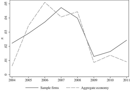
Price changes in sample and in the aggregate economy. The solid line shows the average annual firm-product inflation rate in our sample and the dashed line the annual change in the aggregate producer price index for the entire goods-producing economy (SNI/NACE sections A– E). We calculate the latter as the log change in the annual average of the monthly values of the producer price index. Source: Statistics Sweden and authors’ calculations.
Descriptive statistics.
| Mean | Median | SD | Pct. 25 | Pct. 75 | No. obs. | |
|---|---|---|---|---|---|---|
| A. Price and quantity variables (2004–2011) | ||||||
| Firm-product inflation rate (πi, p, t) | 0.029 | 0.007 | 0.159 | −0.031 | 0.093 | 45,953 |
| Change in quantity sold (ΔQi, p, t) | −0.007 | 0.005 | 0.442 | −0.147 | 0.154 | 45,953 |
| Change in unit input costs (ΔUICi, p, t) | 0.033 | 0.024 | 0.261 | −0.080 | 0.147 | 45,953 |
| B. Time-invariant firm characteristics (2007) | ||||||
| Trade credit maturity (|$\hat{\tau }_i^{07}$|) | 0.097 | 0.095 | 0.056 | 0.064 | 0.124 | 3,408 |
| |$ {{Inventories/Sales}}_i^{07}$| | 0.142 | 0.124 | 0.110 | 0.069 | 0.189 | 3,408 |
| |$ {{Export \ share}}_{j(i)}^{07}$| | 0.299 | 0.251 | 0.232 | 0.086 | 0.433 | 3,408 |
| |$ {{Cash/Assets}}_i^{07}$| | 0.083 | 0.024 | 0.127 | 0.002 | 0.112 | 3,408 |
| |$ {{Unused \, LC/Assets}}_i^{07}$| | 0.043 | 0.003 | 0.070 | 0.000 | 0.062 | 3,408 |
| ΔCustPDc(i) | 0.708 | 0.651 | 0.134 | 0.628 | 0.749 | 3,408 |
| ΔSalesc(i) | −0.070 | −0.047 | 0.103 | −0.125 | −0.008 | 3,408 |
| |$\Delta {Sales}_{c(i)}^{IV}$| | −0.042 | −0.057 | 0.037 | −0.072 | −0.002 | 3,408 |
| ΔSumInji | 0.115 | 0.000 | 0.744 | 0.000 | 0.000 | 3,408 |
| ΔNoInji | 0.110 | 0.000 | 0.715 | 0.000 | 0.000 | 3,408 |
| C. Time-varying firm characteristics (2004–2011) | ||||||
| Trade credit maturity (|$\hat{\tau }_{i,t}$|) | 0.090 | 0.090 | 0.048 | 0.060 | 0.117 | 18,025 |
| Cash/Assetsi, t | 0.081 | 0.022 | 0.124 | 0.002 | 0.111 | 18,025 |
| Bank debt/Assetsi, t | 0.126 | 0.028 | 0.164 | 0.000 | 0.232 | 18,025 |
| Tangible assets/Assetsi, t | 0.269 | 0.248 | 0.183 | 0.116 | 0.392 | 18,025 |
| Cash flow/Assetsi, t | 0.125 | 0.122 | 0.131 | 0.057 | 0.198 | 18,025 |
| Inventories/Salesi, t | 0.148 | 0.128 | 0.105 | 0.078 | 0.194 | 18,025 |
| Assetsi, t (in SEK 1,000) | 318,984 | 58,994 | 1,018,467 | 26,518 | 164,564 | 18,025 |
| Salesi, t (in SEK 1,000) | 390,197 | 101,013 | 1,003,049 | 45,561 | 258,046 | 18,025 |
Notes: This table reports descriptive statistics for all variables used in the empirical analysis, as well as for some additional firm characteristics. Each firm appears only once in panel B and only once per year in panel C, irrespective of how many products it sells and thus how many firm-product observations it has in a given year. Definitions of the variables are provided in the text.
In Figure 2, finally, we document an important feature of trade credit maturities that will help inform our conceptual framework and empirical approach, namely, that maturities are persistent over time. More specifically, the figure plots average trade credit maturities, as measured by |$\hat{\tau }_{i,t}$|, for firms above and below the sample medians of |$\hat{\tau }_{i,t}$| and |$\hat{\tau }_{i}^{07}$|, respectively. Average trade credit maturities are very stable over the period 2004–2011 for both above- and below-median firms when using the yearly classification, whereas above-median firms, as classified based on |$\hat{\tau }_{i}^{07}$|, reduced maturities slightly during the crisis, with |$\hat{\tau }_{i,t}$| falling from 0.129 to 0.112.
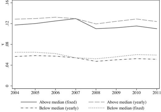
Average trade credit maturities over time. The figure shows average trade credit maturities, as measured by |$\hat{\tau }_{i,t}$|, for firms above and below the sample medians of |$\hat{\tau }_{i,t}$| and |$\hat{\tau }_{i}^{07}$|, respectively, over the period 2004–2011. The solid and short-dashed lines show average maturities when the classification of firms is done on a year-by-year basis (|$\hat{\tau }_{i,t}$|), and the long-dashed and dashed-dotted lines when the classification is done based on the trade credit maturity distribution in 2007 (|$\hat{\tau }_{i}^{07}$|).
3. Conceptual Framework and Empirical Approach
3.1. Conceptual Framework
Since lending is associated with costs—most importantly due to funding and to credit risk exposure—prices charged in trade credit transactions likely surpass prices charged in cash transactions. Schwartz (1974) highlights this trade credit feature of price setting and suggests that firms add a trade credit premium to the cash price, determined by the contracted loan maturity and an implicit interest rate, in transactions involving trade credit. Our conceptual framework rests on the relationship proposed by Schwartz and we focus on its implications for the link between firms’ trade credit issuance and pricing decisions.
In line with Schwartz (1974), our hypothesis is that the trade credit interest rate, r, is determined by two factors: (i) the seller’s cost of liquidity and (ii) the risk of the buyer’s default in the transaction.10 That is, the implicit interest rate in product prices is increasing in sellers’ liquidity costs and credit risk exposures, all else equal. The cost of liquidity that applies to the issuance of trade credit is given by the opportunity cost of the marginal unit of liquidity facing a firm—the shadow cost of liquidity—and is thus equal to the external funding cost for financially unconstrained firms, but higher than this for firms that experience binding liquidity constraints due to external finance rationing (Whited 1992). Regarding counterparty risks, the Bankruptcy Code in Sweden provides trade credit debt with junior priority status, which means that sellers have little hope of recovering claims on failed buyers’ bankruptcy estates after prioritized holders of claims have been handled (Thorburn 2000).11 Hence, trade credit lending is associated with substantial credit risk (see Jacobson and von Schedvin (2015), for further empirical evidence on this).
3.2. Baseline Specification
The parameter of interest is β, which captures the difference between crisis and noncrisis years in the extent to which trade credit maturities affected firm-product inflation rates. In particular, on the basis of equation (4) and its embedded assumption of persistence over time in τ, |$\hat{\beta }$| provides an estimate of the difference in Δr between crisis and noncrisis years. Our empirical approach is thus based on the aggregate shocks to liquidity costs and counterparty risk arising in the 2008–2009 recession in Sweden, in combination with the cross-sectional variation in trade credit maturities that prevailed at the outset of this period.12 The underlying idea is twofold. First, as noted previously, the 2008–2009 recession in Sweden featured general and widespread increases in liquidity costs and counterparty risks, which, according to the hypothesis outlined in the previous section, should lead to upward shifts in implicit trade credit interest rates, ri, p. The crisis dummy is thus a proxy that captures the fact that changes in the underlying determinants of ri, p were higher in crisis years than in noncrisis years. Second, an increase in ri, p of a given size will have a greater impact on product prices set by firms that issue trade credit with longer maturities, in accordance with equation (4). Hence, within this framework we can test if product prices include a trade credit price premium by comparing firm-product inflation rates across crisis and noncrisis years, respectively, for firms that issue trade credit with long and short maturities.
3.3. Potential Threats to Identification
The identifying assumption underlying the empirical specification detailed in the previous section is that there are no omitted variables correlated with the interaction term |${\textit {Crisis}}_t \cdot \hat{\tau }_i^{07}$| that affect firm-product inflation rates, conditional on controls. This implies that a potential omitted variable needs to fulfill two conditions to be of concern: it has to be correlated with |$\hat{\tau }_i^{07}$| and its effect on firm-product inflation rates must vary between crisis and noncrisis years. Now, since our identifying variation is given by the cross-sectional differences in trade credit maturities that prevailed at the outset of the crisis, |$\hat{\tau }_i^{07}$|, and not by variation stemming from an exogenous shock, it is important to probe the sources of the variation in maturities. To this end, we compare firms with average trade credit maturities above and below the sample median, respectively, on all firm-level covariates used in the empirical analysis, measured in 2007. The comparison is conducted on the basis of four measures of covariate balance proposed by Imbens and Rubin (2015): normalized differences in means, logs of the ratios of standard deviations, and two measures of coverage frequency. The results of this comparison, presented in Table 2, show that firms issuing trade credit with long and short maturities are similar across the entire set of covariates under consideration.13 This is consistent with the findings in the previous literature, which has struggled to provide unambiguous evidence regarding the determinants of variation in trade credit maturities across sellers (see Ellingsen, Jacobson, and von Schedvin 2016 for empirical evidence and a review of the literature).
Covariate balance in the sample.
| A. High |$\hat{\tau }_i^{07}$| | B. Low |$\hat{\tau }_i^{07}$| | C. Covariate balance measures | ||||||
|---|---|---|---|---|---|---|---|---|
| Mean | SD | Mean | SD | Δh − l | Γh/ℓ | |$\pi _h^{.95}$| | |$\pi _\ell ^{.95}$| | |
| |${{Cash/Assets}}_i^{07}$| | 0.076 | 0.112 | 0.091 | 0.141 | −0.110 | −0.235 | 0.938 | 0.991 |
| |${{Bank \, debt/Assets}}_i^{07}$| | 0.146 | 0.165 | 0.111 | 0.159 | 0.217 | 0.038 | 0.976 | 0.971 |
| |${{Tangible \, assets/Assets}}_i^{07}$| | 0.235 | 0.174 | 0.270 | 0.195 | −0.190 | −0.116 | 0.912 | 0.974 |
| |${{Cash \, flow/Assets}}_i^{07}$| | 0.139 | 0.127 | 0.145 | 0.149 | −0.043 | −0.160 | 0.914 | 0.974 |
| |${{Inventories/Sales}}_i^{07}$| | 0.150 | 0.109 | 0.134 | 0.111 | 0.141 | −0.023 | 0.906 | 0.974 |
| |$\ln ( {Assets}_i^{07})$| | 10.947 | 1.281 | 11.166 | 1.585 | −0.153 | −0.213 | 0.877 | 0.983 |
| |${{Export \, share}}_{j(i)}^{07}$| | 0.305 | 0.229 | 0.293 | 0.234 | 0.052 | −0.019 | 0.950 | 0.966 |
| |${{Unused \, LC/Assets}}_i^{07}$| | 0.047 | 0.071 | 0.039 | 0.068 | 0.115 | 0.045 | 0.977 | 0.974 |
| ΔCustPDc(i) | 0.707 | 0.134 | 0.710 | 0.133 | −0.021 | 0.012 | 0.964 | 0.890 |
| ΔSalesc(i) | −0.083 | 0.100 | −0.056 | 0.105 | −0.264 | −0.048 | 0.856 | 0.955 |
| ΔSumInji | 0.121 | 0.740 | 0.108 | 0.748 | 0.018 | −0.011 | 1.000 | 1.000 |
| ΔNoInji | 0.119 | 0.705 | 0.100 | 0.725 | 0.027 | −0.029 | 1.000 | 1.000 |
| No. firms | 1,752 | 1,656 | ||||||
Notes: This table reports descriptive statistics for firms with average trade credit maturities, |$\hat{\tau }_{i}^{07}$|, above and below the sample median (panels A and B), as well as four measures of covariate balance proposed by Imbens and Rubin (2015) (panel C). The set of covariates comprises all firm-level control variables, measured in 2007, as well as all sample-split variables used in the empirical analysis. Δh − ℓ denotes a normalized difference and is calculated as |$(\bar{X}_h-\bar{X}_\ell) / \sqrt{( S_h^2+S_\ell ^2) /2}$|, where |$\bar{X}$| is the mean, S is the standard deviation, and subindices h and ℓ denote firms with trade credit maturities above and below the sample median, respectively. Γh/ℓ is the log of the ratio of the standard deviations for above-median and below-median firms. Finally, |$\pi _h^{.95}$| measures the share of below-median firms for which the value of a given variable lies in the 95% central range of the distribution of the same variable for above-median firms (and vice versa for |$\pi _\ell ^{.95}$|).
We assess potential threats to the identifying assumption in the following ways. First, we estimate the baseline specification augmented with, in turn, product-year fixed effects and industry-year fixed effects, which means that we effectively compare firms with high and low trade credit issuance selling the same product, or operating in the same industry, in a given year. These specifications thus address threats from the set of potentially confounding factors suggested by theories that posit that trade credit maturities are determined by product- or industry-specific factors (e.g., Lee and Stowe 1993; Long, Malitz, and Ravid 1993; Kim and Shin 2012; Kalemli-Özcan et al. 2014). Second, we estimate the baseline specification augmented with interactions between the crisis variable and specific potential confounders that can vary within product and industry clusters, and which are therefore not absorbed by product-year or industry-year fixed effects. Third, we address an alternative explanation for why trade credit issuance and prices may be positively related during periods of tight credit. Suppose that demand increases for goods sold by firms issuing trade credit with longer maturities as a consequence of trade credit becoming more valuable for buyers when other sources of financing dry up. Increased demand could then push up the prices set by these firms relative to the prices of firms that provide short maturities. To distinguish between the demand- and supply-side explanations, we estimate a version of the baseline specification with changes in the quantities of goods sold replacing changes in prices as outcome variable; if the explanation based on demand is correct, we should observe an increase in both prices and quantities for goods sold by firms that issue long trade credit maturities, whereas we would observe higher prices, but lower or unchanged quantities if the effects are supply-driven.
4. Main Results
We begin the presentation of our empirical findings with a graphical illustration of our main result. Figure 3 shows average firm-product inflation rates over the period 2004–2011 for firms with average trade credit maturities above (solid line) and below (dashed line) the sample median in year t − 1. Inflation rates for the two groups of firms track each other closely in the four years leading up to the 2008–2009 recession, but then differ markedly during the crisis: although the average inflation rate falls in both groups of firms—which is what one would expect in a crisis period with deflationary pressures—it falls considerably less among firms that issue long trade credit maturities. In the post-crisis period, the inflation rates in the two groups of firms begin to follow each other more closely again. Figure 3 thus provides illustrative evidence for our hypothesis that increases in liquidity costs and counterparty risk lead firms to raise trade credit premia and thereby product prices. In what follows, we formalize this result by means of the empirical strategy outlined in the previous section.
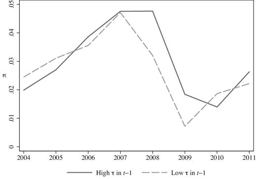
Average firm-product inflation rates over time. The figure shows average firm-product inflation rates in each year of the sample period for firms above (solid line) and below (dashed line) the median of the trade credit maturity distribution in year t − 1, |$\hat{\tau }_{i,t-1}$|.
4.1. Baseline Results and Robustness Checks
Table 3 reports results for various estimations of the model specified in equation (5). We quantify the magnitude of the coefficients for the main explanatory variable, the interaction term |${\textit {Crisis}}_t \cdot \hat{\tau }_i^{07}$|, in two ways. First, we report the coefficients themselves, which, as noted previously, capture the difference in Δr between crisis and noncrisis years. Second, we calculate what the coefficients imply in terms of the difference in annual firm-product inflation rates between firms that issue long and short trade credit maturities by multiplying the coefficient with the difference in |$\hat{\tau }_i^{07}$| between firms located at the 75th and 25th percentiles, respectively, of the |$\hat{\tau }_i^{07}$|-distribution.14
Baseline results.
| (1) | (2) | (3) | (4) | (5) | (6) | (7) | (8) | (9) | (10) | |
|---|---|---|---|---|---|---|---|---|---|---|
| πi, p, t | πi, p, t | πi, p, t | |$\pi _{i,p,t}^{+}$| | πi, p, t | πi, p, t | πi, p, t | πi, p, t | πi, p, t | ΔQi, p, t | |
| |${{Crisis}}_t \cdot \hat{\tau }_i^{07}$| | 0.209*** | 0.154*** | 0.415** | 0.232*** | 0.125** | 0.182*** | 0.214*** | 0.230*** | −0.008 | |
| (3.4) | (3.2) | (2.4) | (3.9) | (2.5) | (3.4) | (3.6) | (3.8) | (−0.1) | ||
| |${{Crisis}}_t \cdot \hat{\tau }_i^{07}, {{High}}$| | 0.018*** | |||||||||
| (2.8) | ||||||||||
| |${{Crisis}}_t \cdot {{Export}} \ {{share}}_{j}^{07}$| | −0.046*** | |||||||||
| (−3.4) | ||||||||||
| |${{Crisis}}_t \cdot {{Inventories/Sales}}_{i}^{07}$| | −0.083*** | |||||||||
| (−2.9) | ||||||||||
| High versus low |$\hat{\tau }_i^{07}$| | 0.013 | 0.009 | — | 0.025 | 0.014 | 0.008 | 0.011 | 0.013 | 0.014 | 0.000 |
| Firm×product FE | Yes | Yes | Yes | Yes | Yes | No | Yes | Yes | Yes | Yes |
| Product×year and firm FE | No | No | No | No | No | Yes | No | No | No | No |
| Industry×year FE | No | No | No | No | No | No | Yes | No | No | No |
| Firm- and product-level controls | Yes | Yes | Yes | Yes | No | Yes | Yes | Yes | Yes | Yes |
| Weights | No | Yes | No | No | No | No | No | No | No | No |
| R2 | 0.429 | 0.420 | 0.429 | 0.319 | 0.214 | 0.590 | 0.458 | 0.430 | 0.429 | 0.306 |
| No. firms | 3,408 | 3,408 | 3,408 | 3,408 | 3,408 | 3,174 | 3,401 | 3,408 | 3,408 | 3,408 |
| No. observations | 45,953 | 45,953 | 45,953 | 45,953 | 45,953 | 35,971 | 45,921 | 45,953 | 45,953 | 45,953 |
Notes: This table reports results for estimations of various specifications based on equation (5). The dependent variable is the firm-product inflation rate, πi, p, t, in all specifications except those in column (4), where it is a dummy equal to one for price increases and zero otherwise, and in column (7), in which it is the change in the quantity of goods sold, ΔQi, p, t. The regression in column (2) is estimated using WLS, where the weight for each observation, ωi, p, t, is calculated as firm i’s sales of product p divided by firm i’s total sales in year t. The product fixed effects are based on 8/9-digit CN codes and the industry fixed effects on three-digit SNI/NACE codes. All regressions include year fixed effects except that in column (7), in which they are redundant. High versus low |$\hat{\tau }_i^{07}$| is calculated as the estimated difference in the dependent variable between firms located at the 75th and 25th percentiles of the |$\hat{\tau }_i^{07}$|-distribution. The estimation period is 2004–2011 in all columns. t-statistics calculated using robust standard errors clustered at the firm-level are reported in parentheses. **Significant at 5%; ***Significant at 1%.
The baseline result is reported in column (1). The coefficient on the interaction term |${\textit {Crisis}}_t \cdot \hat{\tau }_i^{07}$| is positive and statistically significant, which suggests that firm-product inflation rates are increasing in trade credit maturities in the crisis period. The magnitude of the coefficient shows that Δr on average was 20.9 percentage points higher during the crisis than in noncrisis years.15 This estimate implies that the difference in annual firm-product inflation rates between firms that issue long and short trade credit maturities was 1.3 percentage points higher in crisis years than in noncrisis years.
Next, we re-estimate the baseline specification using weights that adjust for differences in the shares of each firm’s total sales accounted for by each of its products. More specifically, we estimate a weighted regression where the weight for each observation, ωi, p, t, is calculated as firm i’s sales of product p divided by firm i’s total sales. Hence, we effectively estimate the baseline regression at the firm level instead of at the firm-product level. The results are reported in column (2). The coefficient on the interaction term |${\textit {Crisis}}_t \cdot \hat{\tau }_i^{07}$| implies a difference in Δr of 15.4 percentage points and a difference in the annual firm-product inflation rate between firms that issue long and short trade credit maturities of 0.9 percentage points, which is slightly lower than in the previous specification. This suggests that sellers with more diversified product portfolios tend to make slightly larger price adjustments on average.
Although we winsorize all variables used in the estimations to reduce the influence of outliers, one may still be concerned that a small number of firms with very long trade credit maturities could influence the results unduly. We therefore estimate a version of the baseline specification in which the main explanatory variable is a dummy indicating whether a firm’s trade credit maturity was above or below the sample median in the last precrisis year. The results, reported in column (3), show that the difference in inflation rates between firms above and below the sample median of the trade credit maturity distribution was 1.8 percentage points higher in crisis years, which is consistent with the baseline result. Similarly, one may be concerned that a small number of very large price adjustments drive the baseline result. To address this, we estimate a version of the baseline specification in which the dependent variable is replaced by a dummy that takes the value one for price increases, and zero otherwise. The coefficient, reported in column (4), implies that the relative propensity of firms that issue long and short trade credit maturities to increase prices was 2.5 percentage points higher in crisis years. These findings suggest that outliers are not a concern for the baseline result.
4.2. Accounting for Alternative Explanations
In the remainder of this section we assess the plausibility of several alternative explanations for our results, by means of variations on the baseline specification. We begin by considering a bivariate regression specification, in which we drop all firm- and product-level control variables except the firm-product and year fixed effects. The purpose is to examine how the inclusion of the control variables in the vectors |${\bf{X}_{i,p,t}}$| and |${\bf{Z}_{i,t-1}}$| affect the baseline estimate, which is helpful for assessing the extent to which unobservables may confound our findings. The results of this exercise are reported in column (5) of Table 3. The point estimate (t-statistic) for the coefficient of interest is 0.232 (3.9), which is very close to the baseline coefficient, whereas R2 drops from 0.429 to 0.214. This indicates that although the firm- and product-level control variables add substantial explanatory power to the regression, their effect on the coefficient of interest is small, which is what one would expect given the similarity of firms that issue high and low trade credit maturities.
Next, the baseline specification includes firm-product fixed effects to control for time-invariant differences in inflation rates across products. Hypothetically, time-varying differences in inflation rates across products could be important: supposing that inflation rates during the crisis were higher for certain products, for reasons unrelated to trade credit issuance, and that the same products are customarily sold with long trade credit maturities, then our baseline result could be spurious. To address this possibility, we estimate a specification in which we replace the firm-product fixed effects with firm fixed effects and product-year fixed effects to control for the part of the variation in the inflation rate that is common to all producers of a given product. The resulting coefficient, reported in column (6), is positive and statistically significant, but its magnitude is only around three-fifths of the magnitude of the baseline coefficient, which suggests that our baseline result is partly associated with time-varying product-specific factors. Note, however, that the sample size falls by more than 20% in this estimation. This reduction occurs because many products are produced by only one firm in a given year and we can only make use of observations belonging to product-year cells with at least two observations in a specification with product-year fixed effects. Hence, the decline in effect magnitude—from 0.209 to 0.125—could be due to some combination of the change in sample composition and the introduction of product-year fixed effects. To test for the sample composition effect, we re-estimate the baseline specification on the subsample comprising observations belonging to product-year cells with at least two observations. This yields a coefficient estimate of 0.168 (3.4), which indicates that one half of the decline in the estimated coefficient can be attributed to the sample composition effect and the other half to the introduction of product-year fixed effects.
On a related note, we assess whether time-varying differences in inflation rates across industries could affect our results. We do this by estimating the baseline specification augmented with industry-year fixed effects, where industries are defined using two-digit SNI/NACE codes. The coefficient on the interaction term |${\textit {Crisis}}_t \cdot \hat{\tau }_i^{07}$|, reported in column (7), implies a difference in Δr of 18.2 percentage points and in the annual firm-product inflation rate between firms that issue long and short trade credit maturities of 1.1 percentage points.
The collapse of world trade that occurred during the global financial crisis had a large adverse impact on Sweden, a small open economy in which exports account for almost half of GDP. This could potentially influence our results, since (i) international trade typically is associated with longer trade credit maturities and (ii) exporting firms faced a substantial drop in demand during the crisis. We control for the potential influence of export demand by augmenting the baseline specification with an interaction term between the crisis dummy and a variable measuring the precrisis export share of total sales at the five-digit industry level, |${\textit {Export}}\ {\textit {share}}_j^{07}$|. The results of this estimation, reported in column (8), show that the coefficient on trade credit maturities is virtually unchanged compared with the baseline specification, whereas the coefficient on the export share is negative and statistically significant, which is what one would expect given the large decline in export demand during the crisis.
Next, some theories of trade credit predict that accounts receivable are negatively correlated with inventory holdings (see, e.g., Bougheas, Mateut, and Mizen 2009). Such a correlation could give rise to bias in our baseline estimates, if the size of a firm’s inventory holdings has a direct impact on its price setting during economic downturns. To examine this possibility, we estimate a version of the baseline specification in which the ratio of precrisis inventories to sales interacted with the crisis dummy is included as a control variable. The results of this estimation are reported in column (9). The coefficient for trade credit maturity is slightly larger than the baseline estimate, whereas the coefficient for inventories is negative and statistically significant, which suggests that firms that entered the crisis with high inventory holdings attempted to reduce these through price cuts. The different signs of the estimated effects of trade credit and inventories indicate that the mechanism that we document in this paper is specific to trade credit provisioning, and not merely an instance of a more general working capital channel.
Finally, another conceivable alternative explanation for our baseline finding is that it reflects a shift in demand during the crisis—away from sellers that issue short trade credit maturities and toward sellers that issue long maturities—as a result of longer trade credit maturities becoming more valuable for liquidity-constrained buyers during crises. To evaluate the demand-shift explanation, we regress the change in the quantity of sold goods, ΔQi, p, t, on the right-hand side of the baseline specification. The idea is that an upward shift in demand for goods sold by firms that issue long trade credit maturities should cause an increase in both prices and quantities. column (10) shows, however, that the coefficient in this specification is negative and insignificant, which speaks against the alternative explanation based on shifts in demand.
5. Mechanisms
In this section we propose to scrutinize the underlying mechanisms for the baseline finding that firms issuing longer trade credit maturities tended to raise product prices more during the crisis. Thus, we conjecture—in accordance with the hypothesis outlined in the conceptual framework—that the association between trade credit issuance and price changes is stronger for firms subject to larger increases in liquidity costs and counterparty risk. To this end, we conduct cross-sectional heterogeneity analyses, in which we estimate the baseline specification on subsamples of firms defined by proxies for changes in liquidity costs and counterparty risk during the crisis. The proxies we use capture firm characteristics obtaining in the crisis and we therefore restrict the sample period to 2006–2009 throughout this section.
5.1. The Liquidity-Cost Mechanism
We use two approaches to identify firms that experienced particularly large increases in liquidity costs during the crisis. First, we follow a common practice in the literature and identify firms based on precrisis characteristics that are likely to have been important determinants of their liquidity costs during the crisis. Second, we use the Baltic crisis and its detrimental effect on two Swedish banks as a quasi-experiment along the lines of Chodorow-Reich (2014).
5.1.1. Results Based on Precrisis Characteristics
We consider two measures of firms’ precrisis liquidity positions as sources of heterogeneity in liquidity costs across sellers during the crisis: cash and liquid assets, |${\textit {Cash}}/{\textit {Assets}}_{i,t-1}^{07}$|; and the size of unused credit lines, |${\textit {Unused}} \ {\textit {LC/Assets}}_{i,t-1}^{07}$|. For each variable, we construct two subsamples: one with the firms in the bottom three deciles and one with the firms in the top three deciles, the former of which corresponds to firms experiencing large increases in liquidity costs during the crisis, and the latter to firms for which this increase was smaller.16 The presumption underlying this exercise is that firms with weaker precrisis liquidity positions were more vulnerable to deteriorations in cash flow and access to external finance during the crisis, and therefore subject to larger increases in liquidity costs (see, e.g., Duchin, Ozbas, and Sensoy 2010; Gilchrist et al. 2017). Hence, we should observe a stronger relationship between trade credit maturities and price changes during the crisis in the group of vulnerable firms.
The results of the exercises based on firms’ precrisis liquidity positions are reported in panel A of Table 4. column (1) covers results for the sample splits based on the |${\textit {Cash}}/{\textit {Assets}}_{i,t-1}^{07}$| distribution. The coefficient is large and statistically significant for firms with low precrisis cash holdings, but small and statistically insignificant for firms with high precrisis cash holdings; the difference is statistically significant at the 1% level in a one-sided test. A similar pattern emerges in column (3), where we report the results for subsamples of firms with credit lines in the bottom and top of the |${\textit {Unused}} \ {\textit {LC/Assets}}_{i,t-1}^{07}$| distribution: the coefficient is large and significant in the former group, but smaller and insignificant in the latter; the difference is in this case statistically significant at the 10% level. These results thus support the notion that increases in liquidity costs partly account for the baseline relationship between trade credit issuance and price changes.
Mechanism I—Liquidity cost pass-through.
| (1) | (2) | ||
|---|---|---|---|
| |${{Cash/Assets}}_{i}^{07}$| | |${{Unused \, LC/Assets}}_{i}^{07}$| | ||
| Panel A. Precrisis balance-sheet measures | |||
| |${\textit{Crisis}}_t \cdot \hat{\tau }_i^{07} \cdot {\mathbb 1} \lbrace T_i \ge T^{70th} \rbrace$| | 0.024 | 0.081 | |
| (0.2) | (0.7) | ||
| |${\textit{Crisis}}_t \cdot \hat{\tau }_i^{07} \cdot \mathbb {1} \lbrace T_i \le T^{30th} \rbrace$| | 0.508*** | 0.307*** | |
| (4.3) | (3.3) | ||
| p-value for difference | 0.005 | 0.070 | |
| R2 | 0.246 | 0.262 | |
| No. firms in top/bottom deciles | 770/783 | 799/1,001 | |
| No. observations | 12,248 | 13,436 | |
| (1) | (2) | (3) | |
| All firms | Single-bank firms | Single-bank firms, not with D | |
| Panel B. The Baltic crisis experiment | |||
| |${\textit{Crisis}}_t \cdot \hat{\tau }_i^{07} \cdot \mathbb {1} \lbrace T_i=0 \rbrace$| | 0.210** | 0.192* | 0.172 |
| (2.1) | (1.7) | (1.3) | |
| |${\textit{Crisis}}_t \cdot \hat{\tau }_i^{07} \cdot \mathbb {1} \lbrace T_i=1 \rbrace$| | 0.398** | 0.492*** | 0.492*** |
| (2.3) | (3.4) | (3.4) | |
| p-value for difference | 0.171 | 0.049 | 0.049 |
| R2 | 0.518 | 0.528 | 0.526 |
| No. control/treated firms | 1,321/643 | 1,003/551 | 748/551 |
| No. observations | 16,574 | 11,668 | 10,003 |
Notes: This table reports results for estimations of equation (5) on various subsamples of firms for the period 2006–2009. Column (1) in panel A reports results for estimations on subsamples consisting of firms in the top three and bottom three deciles, respectively, of the |${\textit {Cash}}/{\textit {Assets}}_{i,t-1}^{07}$| distribution, whereas column (2) reports results for a corresponding sample-split based on the |${\textit {Unused}} \ {\textit {LC/Assets}}_{i,t-1}^{07}$| distribution. The cutoffs used to construct the subsamples are defined at the firm level; hence, the number of firms in each subsample is approximately the same, whereas the number of observations differ somewhat (note, though, that the number of firms differs somewhat in the split based on credit lines due to the fact that more than 30% of firms have no unused credit line). Columns (1)–(3) in panel B concern estimations of equation (5) on treated firms and control firms in the Baltic crisis experiment. The samples underlying the estimations in the three columns comprise all firms with a precrisis bank relationship (column 1); all single-bank firms (column 2); and single-bank firms except those with bank D as their main lender (column 3). Reported p-values correspond to one-sided tests, where the null hypothesis is that the estimates of β are equal in each pair and the alternative hypothesis that the coefficients are larger for firms in the bottom deciles (panel A) and in the treatment group (Panel B). t-statistics calculated using robust standard errors clustered at the firm-level are reported in parentheses. *Significant at 10%; **significant at 5%; ***significant at 1%.
5.1.2. The Baltic Crisis as a Quasi-Experiment: Empirical Setup
In search of a possibly more exogenous source of variation in liquidity costs, we now turn to the Baltic crisis and its effect on Swedish banks’ corporate lending, following the empirical approach of Chodorow-Reich (2014). The idea is that bank–firm relationships are sticky, and that variation in loan supply across banks therefore gives rise to variation in access to external finance across firms.17 In our context, this implies that the cross-sectional variation in bank health caused by the Baltic crisis gave rise to variation in liquidity costs across Swedish nonfinancial firms. Hence, by splitting our sample based on which bank served each firm as its main lender at the outset of the crisis, we obtain subsamples consisting of firms for which the increase in liquidity costs during the crisis was larger and smaller, respectively. In what follows, we describe the relevant features of the Baltic crisis in more detail and explain how we exploit it as a quasi-experiment.18
The Swedish bank market is dominated by four major banks, which we refer to as banks A, B, C, and D. These four banks operate countrywide and lend to households and firms in all sectors of the Swedish economy; at the time of the crisis, they accounted for about 85% of banking sector assets and 75% of corporate lending. Prior to the global financial crisis, all of these banks had entered the Baltic market, but the scale of their Baltic operations differed greatly, with two banks (C and D) having substantial shares of their loan portfolios allocated to the Baltic market, whereas the other two had only minor (bank B) or even negligible (bank A) shares of their lending there. The Baltic countries subsequently suffered among the deepest recessions in the world during the crisis, which led to large losses for banks operating in the region. The impact of the crisis differed substantially across Swedish banks, causing large losses for banks C and D, whereas leaving banks A and B more or less unharmed. This quickly led financial market participants to revise their assessments of the two exposed banks, which put immediate pressure on their funding situations. Panels (a) and (b) of Figure 4 show CDS spreads and stock prices, respectively, for the four major Swedish banks between 2007 and 2010; whereas CDS spreads increased and stock prices fell for all banks during the crisis, they did so more drastically for banks C and D. There is widespread agreement that these differences are accounted for by the banks’ differential exposures to the Baltic countries (see, e.g., Ingves 2010; Bryant, Henderson, and Becker 2012; IMF 2012).
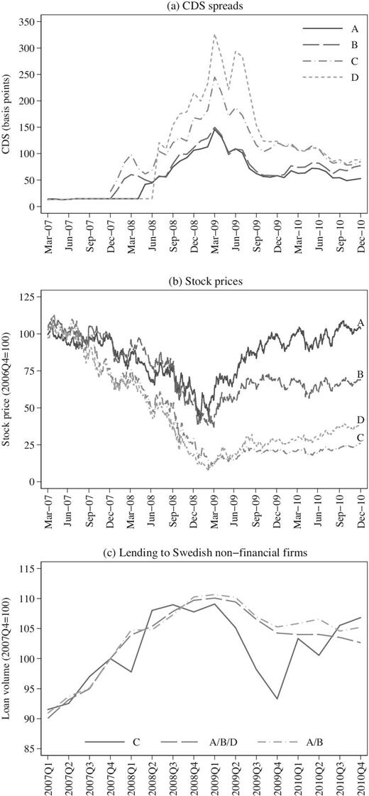
Swedish banks and the Baltic crisis. The figure shows five-year senior unsecured CDS spreads (panel (a)); stock prices (panel (b)); and the total volume of outstanding loans to Swedish nonfinancial firms (panel (c)) for the four major Swedish banks between 2007 and 2010. The dashed line in panel (c) shows the joint loan volumes of banks A, B, and D, and the dashed-dotted line the joint loan volumes of banks A and B. Sources: Thomson Reuters and Statistics Sweden.
Swedish authorities responded by swiftly implementing several crisis measures intended to mitigate the impact of the crisis on the banking sector. The most important response was the introduction of a guarantee program that offered full government insurance for all new debt issued by banks that chose to opt into the program. To participate in the program and receive the insurance, a bank had to pay a fee—amounting to 50 basis points for debt with maturities less than a year, and the bank’s average precrisis CDS spread plus 50 basis points for debt with longer maturities—as well as adhere to certain conditions, for example, that no bonuses could be paid out to senior management while the bank participated in the program. The design and scope of the program implied that participating banks could borrow cheaply during the crisis, since the precrisis CDS spreads were low for all banks and the government insurance made lending virtually risk-free for creditors.
In the end, however, only the bank most affected by the Baltic crisis (bank D) chose to participate, which meant that it was only the second-most affected bank (bank C) that saw its actual funding costs rise sharply during the crisis. As Chodorow-Reich (2014) and others point out, adverse shocks to bank health primarily reduce credit supply by increasing banks’ funding costs; hence, the Baltic crisis only affected bank C in the sense that we are interested in here.19 One would thus expect bank C to have reduced lending more than the other banks during the crisis. In panel (c) of Figure 4, we show that this is precisely what happened. This suggests that borrowers of bank C on average faced a contraction in loan supply relative to borrowers of banks A, B, and D.
We exploit the Baltic crisis as a quasi-experiment by assigning firms whose main precrisis lender was bank C to a treatment group and firms whose main lender was bank A, B, or D to a control group.20 In this setting we can test the hypothesis that the relationship between trade credit maturities and price changes during the crisis is stronger for firms in the treatment group, that is, for firms who saw their access to external finance decline more during the crisis.
5.1.3. The Baltic Crisis as a Quasi-Experiment: Results
The results for the Baltic crisis quasi-experiment are presented in panel B of Table 4. The first row shows the estimated coefficients for control firms (Ti = 0) and the second row the coefficients for treated firms (Ti = 1). Consider first column (1), in which we present the results of the estimation of the specification just described, in which the treatment group consists of all firms whose precrisis main lender was bank C and the control group of all firms whose main lender was bank A, B, or D. The results show that the coefficient of interest is more than twice as large for treated firms as for control firms, but the difference between the two subsamples is despite this not statistically significant. Hence, these results provide some support for our conjecture, but the evidence is not conclusive.
Note, however, that although all treated firms had bank C as their main lender at the outset of the crisis, some of them had active relationships with other banks as well, and could therefore likely offset some part of the contraction in lending on the part of bank C by increasing borrowing from their other banks. If so, some firms that were not in fact affected by the negative loan supply shock would be included in the treatment group, which would weaken the test. We therefore consider an alternative specification, in which we drop all multiple-bank firms from the treatment group as well as from the control group (the latter to avoid introducing differences in the characteristics of treated firms and control firms). The results in column (2) show that the difference in the estimated coefficients becomes even larger, 0.492 versus 0.192, when we consider single-bank firms only; moreover, the difference is now statistically significant at the 5% level.
Finally, although bank D participated in the guarantee program and thereby largely avoided the effects of the crisis on its funding costs, it is still possible that its lending behavior was affected by the crisis. We therefore consider a specification that is equivalent to that in column (2), except that the control group only includes firms whose main precrisis lender was bank A or B. The results of this alternative specification, reported in column (3), are, however, very similar to the results in column (2); hence, whether or not borrowers of bank D are included in the control group matters little for the results. In sum, the results of the analysis based on the Baltic crisis lends further support to the claim that increases in liquidity costs is a mechanism underlying the positive relationship between trade credit issuance and price changes during the crisis.
5.2. The Counterparty-Risk Mechanism
We turn next to the evidence for the counterparty-risk mechanism. For want of data at the level of buyer–seller pairs—which would allow us to the estimate the relationship between buyer risk and product prices directly, while controlling for seller characteristics using seller fixed effects—we rely on the following proxies for the change in counterparty risk facing each seller during the crisis: first, a set of industry-level measures of buyer risk calculated using input–output tables; and second, seller-level measures constructed using data on applications for the issuance of injunctions to enforce late trade credit payments, submitted by sellers to the Swedish Enforcement Agency.
5.2.1. Results Using Industry-Level Measures of Counterparty Risk
We use two main industry-level measures of changes in counterparty risk during the crisis, one based on changes in the average default probability (PD) of firms in buyer industries, |$\Delta {\textit {CustPD}}_{c(i)}$|, and the other based on changes in sales in buyer industries, |$\Delta {\textit {Sales}}_{c(i)}$|. Although the former is a direct measure of shifts in counterparty risk, the latter is a broader measure intended to capture risk shifts induced by weakening demand during the crisis. |$\Delta {\textit {CustPD}}_{c(i)}$| is constructed as follows: first, we calculate the sales-weighted average default probability for each two-digit SNI/NACE industry and year; we then compute the change in each industry’s weighted average PD between 2007 and 2009; finally, we use the 2008-vintage of Statistics Sweden’s input–output tables to calculate the industry-level measure of changes in average buyer PDs facing firms in each industry. Based on |$\Delta {\textit {CustPD}}_{c(i)}$|, we then construct two subsamples: one comprising firms in the top three deciles and one firms in the bottom three deciles, respectively. The former consists of firms that faced a larger increase in counterparty risk during the crisis, and the latter of firms for which this increase was smaller.
Our second industry-level measure, |$\Delta {\textit {Sales}}_{c(i)}$|, is constructed by first computing the change in sales between 2007 and 2009 at the two-digit industry level, and then using the input–output table to convert the industry sales changes to a measure of sales growth at the level of buyer industries. We then construct subsamples by assigning firms for which |$\Delta {\textit {Sales}}_{c(i)}$| is less than or equal to zero to one group, and firms for which it is positive to another; the former consists of firms with larger and the latter of firms with smaller increases in counterparty risk during the crisis.
The results for the sample splits based on the main industry-level measures of counterparty risk are reported in columns (1) and (2) of Table 5. In both cases, the estimated coefficient is large and statistically significant in the subsample of firms that faced larger increases in counterparty risk during the crisis, but small and statistically insignificant in the group of firms for which the risk increase was lower; the difference between the coefficients estimated for the two subsamples within each pair is, moreover, statistically significant in both cases. These findings thus support the conjecture that increases in counterparty risk contribute to the positive relationship between trade credit issuance and price changes during the crisis.
Mechanism II—Counterparty risk pass-through.
| (1) | (2) | (3) | (4) | (5) | |
|---|---|---|---|---|---|
| |$\Delta {\textit {CustPD}}_{c(i)}$| | |$\Delta {\textit {Sales}}_{c(i)}$| | |$\Delta {\textit {Sales}}_{c(i)}^{IV}$| | |$\Delta {\textit {SumInj}}_i$| | |$\Delta {\textit {NoInj}}_i$| | |
| |${\textit {Crisis}}_t \cdot \hat{\tau }_i^{07} \cdot \mathbb {1} \lbrace T_i^{\textit {High}}=0 \rbrace$| | 0.016 | 0.393*** | 0.367*** | 0.218*** | 0.210*** |
| (0.1) | (4.5) | (4.3) | (2.7) | (2.7) | |
| |${\textit {Crisis}}_t \cdot \hat{\tau }_i^{07} \cdot \mathbb {1} \lbrace T_i^{\textit {High}}=1 \rbrace$| | 0.515*** | −0.011 | 0.029 | 0.429** | 0.547** |
| (3.4) | (−0.1) | (0.2) | (2.1) | (2.4) | |
| p-value for difference | 0.004 | 0.005 | 0.020 | 0.168 | 0.083 |
| R2 | 0.285 | 0.257 | 0.255 | 0.250 | 0.250 |
| No. firms | 887/792 | 1,980/663 | 2,090/553 | 2,300/343 | 2,316/327 |
| No. observations | 21,091 | 21,091 | 21,091 | 21,091 | 21,091 |
Notes: This table reports results for estimations of equation (5) on various subsamples of firms for the period 2006–2009. More specifically, the different columns report results for sample splits based on the change in buyer PDs (column 1); the change in sales in buyer industries (column 2); the change in sales in buyer industries instrumented using the precrisis export share of each industry (column 3); the change in the sum of the claims underlying the injunctions issued on behalf of each seller (column 4); and the change in the number of injunctions issued on behalf of each seller (column 5). The changes are from 2007 to 2009 in all cases. In column (1), |$T_i^{\textit {High}}$| is equal to zero for firms in the bottom three deciles of the |$\Delta {\textit {CustPD}}_{j(c)}$| distribution, and to one for firms in the top three deciles. In remaining columns, |$T_i^{\textit {High}}$| is equal to zero if Ti ≤ 0 and equal to one if Ti > 0. Reported p-values correspond to one-sided tests, where the null hypothesis is that the estimates of β are equal in each pair and the alternative hypothesis that the coefficients are larger for firms with |$T_i^{\textit {High}}=1$| in columns (1), (4), and (5), and for firms with |$T_i^{\textit {High}}=0$| in columns (2) and (3). The number of firms refer to the numbers of firms for which |$T_i^{\textit {High}}=0$| and |$T_i^{\textit {High}}=1$|, respectively. t-statistics calculated using robust standard errors clustered at the firm-level are reported in parentheses. **Significant at 5%; ***significant at 1%.
The analysis so far is based on ex post measures that in principle could be subject to reverse causality. To address this concern, we employ a precrisis instrument for the change in counterparty risk during the crisis, which allows us to construct a sample split based exclusively on ex ante variables. More specifically, we use the precrisis export share of sales for each industry as an instrument for |$\Delta {\textit {Sales}}_{c(i)}$|, since an important cause of the downturn in the Swedish economy during the crisis was the decline in export demand generated by the collapse in international trade. Indeed, an industry-level regression of the log change in sales between 2007 and 2009 on the export share of sales in 2007 yields a point estimate (t-statistic) of −0.345 (–3.7) and an F-statistic of 13.4, which shows that precrisis export share is a strong predictor for sales growth during the crisis. We therefore construct an alternative sales growth measure, |$\Delta {\textit {Sales}}_{c(i)}^{\textit {IV}}$|, in which we substitute the predicted values from the regression of sales growth on precrisis export share for actual sales growth during the crisis. We then run this measure through the input–output table and construct subsamples in precisely the same way as for the original sales growth measure.
The results when estimating equation (5) on the subsamples defined by the distribution of |$\Delta {\textit {Sales}}_{c(i)}^{\textit {IV}}$| are presented in column (3) of Table 5. They are very similar to the results for the original sales growth measure: the coefficient is again large and statistically significant for the group of firms that faced larger increases in counterparty risk, but small and statistically insignificant in the group of firms for which the increase was lower, whereas the difference between the estimated coefficients is statistically significant.
5.2.2. Results Using Data on Injunctions Issued by the EA
The analysis in the previous section relies on industry-level measures of counterparty risk, which by construction are crude approximations for the true changes in risk facing individual firms. We will therefore next consider a seller-level measure of risk, constructed using data provided by the Swedish Enforcement Agency (EA), the government agency tasked with coordinating the administrative process of bankruptcy resolution. One of the responsibilities of the EA is to provide legal support to sellers for the management of their unsettled trade credit claims. More specifically, a seller who holds an overdue trade credit claim on a customer can request the EA to issue an injunction against the customer; if the request is approved, the EA will notify the debtor for payment within a fortnight and take further measures to enforce payment should the debtor persist in dishonoring the claim. The data we have obtained from the EA consists of the complete record of injunctions issued by the EA in response to applications submitted by the universe of Swedish corporate firms from 2007 and onward. Hence, for each seller in our sample, we observe all injunctions that were issued on its behalf in a given year, as well as the sum of the claims they concern. The data on injunctions issued by the EA thus allow us to identify sellers whose buyers are in financial trouble and who therefore constitute particularly large credit risks. Hence, by computing the change in the number of injunctions issued on behalf of a given seller between 2007 and 2009—or, analogously, the change in the sum of the claims underlying the same injunctions—we can identify sellers who faced particularly large increases in counterparty risk during the crisis.21
The analysis based on the injunction data is structured as follows. For each seller, we compute the change in the sum of the claims underlying the injunctions issued on its behalf between 2007 and 2009, |$\Delta {\textit {SumInj}}_i$|. We do this using the symmetric growth rate formula, since the number of applications submitted in 2007 is zero for almost all sellers in the sample.22 We then split the sample into two groups—one consisting of firms with a growth rate strictly larger than zero and the other of firms for which the growth rate is less than or equal to zero—and test the hypothesis that the relationship between trade credit maturities and price changes during the crisis is stronger for firms in the former group, that is, for sellers who faced a greater increase in counterparty risk. We also conduct an analogous exercise based on the change in the number of injunctions issued on behalf of each seller between 2007 and 2009, |$\Delta {\textit {NoInj}}_i$|.
The results of the exercises based on |$\Delta {\textit {SumInj}}_i$| and |$\Delta {\textit {NoInj}}_i$| are reported in columns (4) and (5), respectively, of Table 5. The findings are similar across the two specifications: the estimated coefficients are statistically significant in both groups of firms, but are considerably larger for the groups of firms that faced larger increases in counterparty risk. The difference between the coefficients is not significant for |$\Delta {\textit {SumInj}}_i$|, whereas we obtain a p-value of 0.081 in the case of |$\Delta {\textit {NoInj}}_i$|. The exercises based on the injunction data thus provide further support for the conjecture that increases in counterparty risk is one mechanism underlying the baseline result.
6. Conclusions
Schwartz (1974) proposes that product prices include a trade credit price premium, determined by the contracted loan maturity and an implicit interest rate, which, in turn, is a function of the selling firm’s liquidity costs and the buying firm’s default risk. This implies that changes in liquidity costs and counterparty risks cause changes in product prices, and thus that trade credit issuance introduces a countercyclical element into firms’ price-setting behavior. We test this proposition empirically using Swedish manufacturing firm data and the 2008–2009 recession as a shock to liquidity costs and counterparty risks.
Our analysis confirms that price adjustments are positively related to trade credit issuance during the crisis: our baseline estimate indicates that the annual change in the implicit trade credit interest rate was 20.9 percentage points higher during the crisis period than in noncrisis years, which implies that a maturity difference of 20 days is associated with a relative annual price adjustment of 1.3 percentage points. By exploring the mechanisms underlying the baseline result, we find evidence that the association between trade credit issuance and price changes during the crisis is stronger for firms that experienced larger increases in liquidity costs and counterparty risks.
Our results relate to several strands of the literature. First, the findings contribute to the trade credit literature by advancing the understanding of how trade credit is priced. In particular, this paper is, to the best of our knowledge, the first to empirically document the existence of implicit interest rates in product prices, which suggests that trade credit is priced even in the absence of explicit interest rates. Second, our results contribute to the macroeconomic literatures on the influence of financial conditions on firms’ price setting, such as the traditional cost channel literature (e.g., Christiano, Eichenbaum, and Evans 1997; Barth and Ramey 2001; Ravenna and Walsh 2006) and the closely related literature studying how liquidity constraints affect price markups in the presence of customer markets (Chevalier and Scharfstein 1996; Gilchrist et al. 2017).
Footnotes
In Sweden, 97% of business-to-business transactions involve trade credit (Pärlhem 2016). Jacobson and von Schedvin (2015) show that the average amount of accounts receivable and payable, scaled by assets, are 16% and 11% for Swedish firms. Similar reliance on trade credit financing prevails across countries. For instance, Rajan and Zingales (1995) show that the corresponding numbers for a sample of US firms are 18% and 15%, whereas Berger and Udell (1998) show that trade credit provides 31% of debt financing to US SMEs, which is nearly as much as commercial banks.
Udell (2015) discusses what he labels “the trade credit pricing puzzle”, and notes that “the ‘all-in’ price—that which matters—must incorporate both the price of the product as well as the financial terms of trade credit. It is highly unlikely that there are any available data that would allow us to calculate this all-in price”.
“2/10 net 30” contracts stipulate that the buyer must pay within 30 days, whereas offering a discount of 2% for payments made within ten days. This implies that buyers are charged an implicit annualized interest rate of 44.6% when they do not avail themselves of the discount offer.
Only a small fraction, around 3%, of Swedish firms use factoring services (Pärlhem 2016).
For US firms, Ng, Smith, and Smith (1999) find that 25.5% of the firms in a sample drawn from Compustat mainly offer two-part contracts, whereas Giannetti, Burkart, and Ellingsen (2011), using the 1998 National Survey of Small Business Finances, document that firms on average are offered early payments discounts from 21.3% of their suppliers. Moreover, Giannetti et al. find that only 7.8% of firms operate in industries in which discounts are common. Using more recent data from 2005, Klapper, Laeven, and Rajan (2012) find that 13% of the contracts extended to a sample of large US and European buyers included early payment discounts. In Sweden, the dominance of net terms contracts over two-part contracts appears to be even larger. For example, Ellingsen, Jacobson, and von Schedvin (2016) find no evidence of the use of two-part contracts in a sample comprising over 50 million trade credit contracts issued by a sample of Swedish suppliers. Moreover, there is no mention of early payments discounts in either of two recent inquiries on trade credit payment terms commissioned by the Swedish government (Bengtsson 2007; Pärlhem 2016).
Note that the argument that product prices may include implicit interest rates also has implications for two-part contracts—the credit extended during the initial period of a two-part contract is commonly viewed as a zero-cost loan, but this credit could also be priced through an implicit interest rate.
These data have previously been used by Carlsson and Skans (2012). To give an idea of the granularity of the product classification, we can, for example, compare the codes 84212100 and 84212200, which refer to “machinery and apparatus for filtering or purifying water” and “machinery and apparatus for filtering or purifying beverages (excl. water)”, respectively.
A firm’s accounts receivable is the sum of all claims held by the firm on its customers for goods and services that have been delivered but not paid. Hence, it measures the total amount of trade credit extended by a firm to all of its customers at a given point in time. By dividing accounts receivable by sales, one obtains a proxy for the average maturity of the trade credit issued by a given firm, measured in years. More precisely, |$\hat{\tau }_i^{07}$| measures average time to payment, which may differ from contracted payment time due to either late or premature payments. Note that value-added tax (VAT) is included in accounts receivable as reported on firms’ balance sheets, but not in the sales figures on the profit-and-loss statements. Hence, the amount of receivables observed for a given firm-year observation needs to be divided by one plus the applicable VAT rate for |$\hat{\tau }_i^{07}$| to capture the true average maturity (the standard VAT rate in Sweden is 25%, but for a few of the industries in our sample, a lower VAT rate of 12% applies).
We do not observe labor costs and intermediate input costs at the product level, so we must resort to the following approximation when calculating |$\Delta {\textit {UIC}}_{i,p,t}$|. For each plant and year, we portion out plant-level labor costs and intermediate input costs across the products produced at the plant in proportion to the plant-level sales share of each product. We then compute the plant-product level values of |$\Delta {\textit {UIC}}_{i,p,t}$|. Finally, we aggregate |$\Delta {\textit UIC}_{i,p,t}$| to the firm-product level using total sales for each product-plant as weights.
Antitrust legislation may to some extent limit firms from engaging in price discrimination. Similarly to the US setting, EU Competition Law (Article 82(c) of the EC Treaty) dictates what Swedish firms can and cannot do in terms of setting differential prices across buyers, and under what circumstances. Whereas it is true that firms cannot fully customize prices—although Article 82(c) has quite strict and precise requirements for making a case of price discrimination—free pricing is not a prerequisite for our analysis, neither conceptually, nor empirically. Indeed, the average interest rate and maturity parameters in equation (2) are consistent with firms setting standardized prices equal for all their buyers on the basis of the opportunity costs of liquidity they face and the average counterparty risks in the pool of buyers they service.
This treatment of trade creditors in bankruptcy proceedings is similar to international practice (see Cuñat and Garcia-Appendini 2012 for an overview).
In exploiting an aggregate shock combined with cross-sectional variation in firms’ exposure to the shock, our empirical set-up is similar to those used in several papers in the previous literature on the financial crisis of 2008–2009, such as Duchin, Ozbas, and Sensoy (2010), Garcia-Appendini and Montoriol-Garriga (2013), and Gilchrist et al. (2017).
To see this, note that the largest normalized difference is 0.26 in absolute terms, whereas the lowest coverage frequency is 0.86. As a comparison, Imbens and Rubin (2015), in an evaluation of the experimental LaLonde (1986) data set, observe a maximum normalized difference of 0.30 and a minimum coverage frequency of 0.91, which they judge to be excellent covariate balance.
The difference between the 75th and the 25th percentiles of the |$\hat{\tau }_i^{07}$|-distribution is 0.060, which corresponds to a difference in trade credit maturity of around 22 days. Throughout the rest of this section, we refer to firms located at the 75th and 25th percentiles of the trade credit maturity distribution as firms that issue long and short trade credit maturities, respectively.
We obtain virtually the same point estimate, 0.211 (3.4), when we estimate the baseline specification with lagged, time-varying trade credit maturities, |$\hat{\tau }_{i,t-1}$|, instead of the time-invariant explanatory variable, |$\hat{\tau }_i^{07}$|.
We only observe lending from the four major Swedish banks and will therefore underestimate |$ {\textit{Unused}} \ {\textit{LC/Assets}}_{i,t-1}^{07}$| for firms obtaining credit from minor banks. This will, if anything, lead us to underestimate the difference between the two subsamples.
For more comprehensive overviews of the Baltic crisis, see the European Commission (2010) and Hansson and Randveer (2013). A more thorough description of the Swedish financial system is provided by Sveriges Riksbank (2015). Bryant, Henderson, and Becker (2012), finally, provide a detailed analysis of the Swedish experience during the global financial crisis.
The choices of banks C and D about whether or not to participate in the guarantee program were of course deliberate decisions on the parts of the banks’ leaderships, rather than random outcomes. This is, however, only problematic for our analysis to the extent that these choices were dictated by the characteristics of the banks’ Swedish corporate borrowers. Although there is no consensus on what the determinants of the banks’ choices were, it is unlikely that differences in customer characteristics was one, as there is little sorting between firms and banks in the corporate segment of the Swedish bank market.
Most firms have only one bank relationship at any given point in time and the main lender is then simply the bank with which the firm has a relationship. For firms with multiple bank relationships, the main lender is defined as the bank with the largest amount of lending to the firm at the outset of the crisis. Firms with no banking relationships at all are excluded from the analysis.
Applying for injunctions to settlement is normally the creditor’s last resort and typically occurs when claims have been overdue for extended periods—several weeks, or longer.
For sellers with no application in either 2007 or 2009, the symmetric growth rate is not defined. We assign a growth rate of zero to these firms.
Acknowledgements
Acknowledgments: We thank the editor, three anonymous referees, Mikael Carlsson, Tore Ellingsen, Isiah Hull, Stefan Ingves, Simon Kwan, and Greg Udell, as well as seminar and conference participants at the Federal Reserve Bank of San Francisco, the Swiss Finance Institute at the University of Zürich, Nova School of Business and Economics in Lisbon, BI Norwegian Business School, the CREDIT 2018 Conference in Venice, and Sveriges Riksbank for helpful comments and suggestions. This research was partly carried out while Tor Jacobson was visiting the Reserve Bank of Australia and Erik von Schedvin the Federal Reserve Bank of San Francisco. We gratefully acknowledge the hospitality extended by these institutions. Niklas Amberg thanks Jan Wallanders och Tom Hedelius stiftelse Grant No. W2016-0351:1. An earlier version of this paper was circulated under the title “Trade Credit and Pricing: An Empirical Evaluation”. The opinions expressed in this article are the sole responsibility of the authors and should not be interpreted as reflecting the views of Sveriges Riksbank.
Notes
The editor in charge of this paper was Claudio Michelacci.
