


Abstract
During recent decades, many new models have emerged in pure and applied economic theory according to which agents’ choices may be sensitive to ambiguity in the uncertainty that faces them. The exchange between Epstein (2010) and Klibanoff et al. (2012) identified a notable behavioral issue that distinguishes sharply between two classes of models of ambiguity sensitivity that are importantly different. The two classes are exemplified by the α-maxmin expected utility (MEU) model and the smooth ambiguity model, respectively; and the issue is whether or not a desire to hedge independently resolving ambiguities contributes to an ambiguity-averse agent's preference for a randomized act. Building on this insight, we implement an experiment whose design provides a qualitative test that discriminates between the two classes of models. Among subjects identified as ambiguity sensitive, we find greater support for the class exemplified by the smooth ambiguity model; the relative support is stronger among subjects identified as ambiguity averse. This finding has implications for applications that rely on specific models of ambiguity preference.
1. Introduction
Decision makers (DMs) choosing between acts are said to face ambiguity if they are uncertain about the probability distribution over states of the world. Over the past three decades, a large decision-theoretic literature has developed, inspired partly by the intuitive view that it is often implausible that a DM can confidently select a single probability distribution over states of the world to summarize her uncertainty, so ambiguity is ubiquitous for decision making in the real world. This literature, reviewed, for example, by Etner et al. (2012) and Gilboa and Marinacci (2013), also draws important inspiration from numerous experimental studies, largely built on Ellsberg's (1961) classic examples, which show that subjects often adjust their behavior in response to ambiguity in ways that cannot be accounted for by subjective expected utility theory (for surveys, see Camerer and Weber 1992; Wakker 2010; Trautmann and van de Kuilen 2015). For instance, many subjects display an ambiguity-averse attitude: intuitively put, being inclined to choose actions whose consequences are more robust to the perceived ambiguity. Recent applied economic theory explores how such departures from subjective expected utility theory in the face of plausible forms of uncertainty may affect a range of economic phenomena.1
The pioneering models in the decision theory literature on ambiguity, and arguably still the most popular, are the Choquet expected utility model of uncertainty aversion introduced in Schmeidler (1989) and the maxmin expected utility (MEU) model of Gilboa and Schmeidler (1989). These models have preference representations that show the DM behaving as if she has a set of probability distributions that she considers possible or relevant. Then, an ambiguity-averse attitude is modelled by having the DM evaluate an act by its minimum expected utility, where the minimum is taken over the set of probability measures considered possible. In a more general version of this classic style of model (α-MEU; Hurwicz 1951; Jaffray 1989; Ghirardato et al. 2004), the DM evaluates acts by considering a weighted average of the minimum and maximum expected utility. More recent theories have brought in preference representations which would allow finer nuances of ambiguity attitude. An important feature that distinguishes the newer vintage models from the earlier ones is that the new models use aggregation rules that do not restrict attention to extreme expected utilities. An example is the smooth ambiguity model of Klibanoff et al. (2005) (hereafter KMM).
Given this theoretical development, a natural question is: Are the features that these newer theories build in empirically compelling? Or, if we were to stick to the classic models of ambiguity-averse behavior, would we miss any empirically important aspect of such behavior? As models in both vintages were designed to capture Ellsberg's classic examples, the many previous experiments based on decisions like those examples do not answer these questions as they do not typically discriminate between the classic and new vintage models. In this paper, we report an experimental study that does so discriminate: the two classes of models predict qualitatively different behavior in our design. Thus, the design discriminates between the MEU/α-MEU family of models and the smooth ambiguity model, arguably the most popular models in applications. As we explain in Section 2.3, this divide is not addressed well in the existing experimental literature.
This is important because, as noted previously, there have been many recent applications of models of ambiguity-sensitive preferences to the understanding of economic phenomena, especially in macroeconomics and financial economics. The typical paper uses a particular preference model, say the MEU model, to explain a phenomenon that is hard to explain plausibly using the standard, expected utility, model. However, some of the explanations depend quite crucially on the particular model of ambiguity sensitivity used. For example, Epstein and Schneider (2010) discuss various applications where MEU works to give the desired result but the smooth model does not because it does not generate kinked indifference curves, as MEU does. On the other hand, some recent applications in the macrofinance area, such as Ju and Miao (2012), Jahan-Parvar and Liu (2014), and Collard et al. (2018), rely on being able to calibrate beliefs and an ambiguity attitude parameter separately, something that can be done in the smooth ambiguity model, but not in the MEU model. Models of ambiguity-averse preference have now also been applied outside macroeconomics and finance, for instance, to climate change policy, where similar issues apply (e.g., the use of the smooth ambiguity model by Millner et al. (2013) and the use of MEU by Chambers and Melkonyan (2017)). Here, too, there is no guarantee that results that hold under one model of ambiguity aversion generalize to other models. The literature is therefore at a point where clearer guidance on the relative empirical performance of these models in particular—and the broader classes that they exemplify—is needed.
Our testing strategy is inspired by the second thought experiment of Epstein (2010) and its generalization in Klibanoff et al. (2012). Our main contribution is to recast the generalized thought experiment as a real operational design, to extend it with additional controls, and to run and report the resulting experiment. The testing strategy is to investigate whether a subject's preference for a randomized act (compared to its pure constituents) is influenced by a desire to hedge across ambiguities in a way that is similar to how diversifying across bets on independent risks hedges those risks. Models of preferences whose representations focus exclusively on the minimum and/or maximum expected utilities in the set considered relevant are uninfluenced by such a desire, in sharp contrast to models whose representations also consider nonextreme expected utilities. Intuitively, a DM focusing only on the minimum expected utility is analogous to an infinitely risk-averse agent caring exclusively about the worst possible outcome and so not about diversifying across independently resolving risks, since such diversification does not affect the possibility of the worst outcome.
For concreteness and to allow the reader to relate easily to the discussions in Epstein (2010) and Klibanoff et al. (2012), we explain our design and results in the main text in terms of the α-MEU and smooth ambiguity models, the divide between which is particularly clear. Appendix C substantiates our claim that the predictions we test also mark a divide between broader classes of models, besides these two. If (as suggested above) ambiguity is ubiquitous in real-world decision making, the importance attached by economists to hedging as a response to uncertainty provides an additional general motivation for our study which goes beyond models, namely, to investigate hedging of ambiguities rather than risks.
The rest of the paper is organized as follows. Section 2.1 describes the α-MEU and smooth ambiguity preference representations; Section 2.2 presents a modified version of Epstein's example and uses it to explain our testing strategy; and Section 2.3 contrasts this strategy with others taken in the literature. Section 3 presents the experimental design, and Section 4 the results, of our main study. Section 5 introduces some issues of robustness and generality, which are examined further in Appendices A, B, and C; it also briefly presents a follow-up study in which one aspect of the design of the main experiment is varied, for reasons explained at that point. Section 6 concludes the main text. An Online Appendix contains further details of the results, experimental procedures, and instructions.
2. Background
2.1. Preference Representations
Formally, the DM’s choices are acts, maps from contingent states of the world to consequences, which include simple lotteries with real outcomes. We focus on two models of preferences over acts: the α-MEU model and the smooth ambiguity model. Each captures the idea that the DM does not know the probabilities of the states by postulating a set of probability measures over the states that she considers possible. The models differ in respect of how that set informs her evaluations of acts.
Although these models have some common features, there are also marked differences between them, one of which drives our testing strategy as we now explain.
2.2. Conceptual Background
Consider the following variant of the second thought experiment proposed in Epstein (2010).2 The DM is told that a ball will be drawn from an urn containing a fixed number of balls, of four different types: B1, B2, R1, and R2. She is also told that the combined number of balls of types B1 and B2 will equal that of balls of types R1 and R2 and, finally but importantly, that the relative proportions within the B-component (B1, B2) and within the R-component (R1, R2) will be determined separately. The DM considers acts with contingent outcomes c, c* and the 50–50 lottery between them. Let c* > c and normalize the utility index u, so that u(c*) = 1 and u(c) = 0. The acts to be considered have state-contingent (expected) utility payoffs as described in Table 1.
Five acts: (expected) utilities.
| B1 | B2 | R1 | R2 | |
|---|---|---|---|---|
| f1 | 1 | 0 | 0 | 0 |
| f2 | 0 | 0 | 1 | 0 |
| mix | |$\frac{1}{2}$| | 0 | |$\frac{1}{2}$| | 0 |
| g1 | |$\frac{1}{2}$| | |$\frac{1}{2}$| | 0 | 0 |
| g2 | 0 | |$\frac{1}{2}$| | |$\frac{1}{2}$| | 0 |
| B1 | B2 | R1 | R2 | |
|---|---|---|---|---|
| f1 | 1 | 0 | 0 | 0 |
| f2 | 0 | 0 | 1 | 0 |
| mix | |$\frac{1}{2}$| | 0 | |$\frac{1}{2}$| | 0 |
| g1 | |$\frac{1}{2}$| | |$\frac{1}{2}$| | 0 | 0 |
| g2 | 0 | |$\frac{1}{2}$| | |$\frac{1}{2}$| | 0 |
To clarify, f1 yields c* when a ball of type B1 is drawn and c otherwise, whereas f2 yields c* when type R1 is drawn and c otherwise. The outcome of the act mix is in part decided by the toss of a fair coin: specifically, for any contingency, there is a 0.5 probability that the outcome is determined by applying f1 and a 0.5 probability that it is determined by applying f2. In what follows, “mixed act” always refers to this mixed act and “constituent acts” refers to f1 and f2 (or, in each case, later to their experimental counterparts). The acts g1 and g2 each yield, in the contingencies for which a cell entry of ½ is shown, either c* or c, depending on the toss of a fair coin (and c otherwise).
How might we expect the DM to choose between these acts? The probability of the event {B1, B2} is objectively known to her and equal to 1/2 (as types B1 and B2 jointly account for half of the balls), but the DM does not know the probability of the event {B2, R1}. Moreover, the information that she has about balls of type B1 exactly matches her information about type R1. Thus, the symmetry in the situation suggests f1 ∼ f2; and, it is natural to expect that, if the DM is ambiguity averse, she will have the strict preference g1 ≻ g2.3
To illustrate the point of contention, it is useful to write down a concrete set of probability measures {p1, …, p4} that we suppose to be those considered by the DM and show in Table 2. In the context of the smooth ambiguity model, think of these as probabilities that are given positive weight by the measure μ and, importantly, with the weights for p2 and p3 equal.
Example probabilities.
| B1 | B2 | R1 | R2 | |
|---|---|---|---|---|
| p1 | |$\frac{1}{{10}}$| | |$\frac{4}{{10}}$| | |$\frac{1}{{10}}$| | |$\frac{4}{{10}}$| |
| p2 | |$\frac{1}{{10}}$| | |$\frac{4}{{10}}$| | |$\frac{4}{{10}}$| | |$\frac{1}{{10}}$| |
| p3 | |$\frac{4}{{10}}$| | |$\frac{1}{{10}}$| | |$\frac{1}{{10}}$| | |$\frac{4}{{10}}$| |
| p4 | |$\frac{4}{{10}}$| | |$\frac{1}{{10}}$| | |$\frac{4}{{10}}$| | |$\frac{1}{{10}}$| |
These measures respect the given information, in that, for each i = 1, 2, 3, 4, pi(B1 ∪ B2) = pi(R1 ∪ R2) = 1/2; and, as p2 and p3 have equal weight, there is complete symmetry between the B-component and the R-component. The measures respect the independence of the two components in that fixing a “marginal” over (B1, B2) does not restrict the “marginal” over (R1, R2), or vice versa. The expected utilities generated by applying each of the measures pi from Table 2 to the acts from Table 1 are as shown in Table 3.
Resulting expected utilities.
| p1 | p2 | p3 | p4 | |
|---|---|---|---|---|
| f1 | |$\frac{1}{{10}}$| | |$\frac{1}{{10}}$| | |$\frac{4}{{10}}$| | |$\frac{4}{{10}}$| |
| f2 | |$\frac{1}{{10}}$| | |$\frac{4}{{10}}$| | |$\frac{1}{{10}}$| | |$\frac{4}{{10}}$| |
| mix | |$\frac{1}{{10}}$| | |$\frac{{2.5}}{{10}}$| | |$\frac{{2.5}}{{10}}$| | |$\frac{4}{{10}}$| |
| g1 | |$\frac{{2.5}}{{10}}$| | |$\frac{{2.5}}{{10}}$| | |$\frac{{2.5}}{{10}}$| | |$\frac{{2.5}}{{10}}$| |
| g2 | |$\frac{{2.5}}{{10}}$| | |$\frac{4}{{10}}$| | |$\frac{1}{{10}}$| | |$\frac{{2.5}}{{10}}$| |
First, consider acts f1 and f2. Their expected utilities coincide under p1 and p4, but differ from each other under p2 and p3. To see why, note from Table 1 that the evaluation of f1 depends on the ratio B1: B2 but not on R1: R2, whereas the evaluation of f2 depends on the ratio R1: R2 but not on B1: B2; and then note, from Table 2, that these ratios coincide under p1 and p4 but not under p2 or p3. In contrast, the evaluation of mix depends on both the ratios, but has half the exposure to the uncertainty about each, compared to each of the constituent acts. The point of contention turns on the significance of these facts.
From the perspective of the α-MEU model, the extremes of the possible expected utilities are what matter for the evaluation of an act. The diversification aspect of the comparison between f1, f2, and mix is irrelevant, because the minimum and maximum possible expected utilities are the same under each of these three acts, as Table 3 shows. So, according to this model, the DM will be indifferent between f1, f2, and mix, regardless of her preference over g1 and g2.
However, from the perspective of the smooth ambiguity model, the mixed act provides a hedging of two separate ambiguities, one involving each of the two components, just as diversifying across bets on independent risks provides a hedging of risks. The benefit of such diversification to an ambiguity-averse DM is captured through a concave |$\phi$|, in that mean-preserving spreads in the subjective distribution of expected utilities generated by an act are disliked. Since p2 and p3 have equal weight, each of f1 and f2 yields a mean-preserving spread in expected utilities compared with mix, as Table 3 shows. Thus, according to the smooth ambiguity model, the mixed act is preferred to its constituents by any ambiguity-averse DM. To generalize, the distinctive prediction of the smooth ambiguity model for the case where p2 and p3 have equal weight is that an ambiguity-averse DM will prefer not just g1 to g2 but also mix to each of f1 and f2, and, correspondingly, an ambiguity-seeking DM (convex |$\phi$|) would have the reverse preference in each case; and an ambiguity-neutral DM (linear |$\phi$|) would be indifferent between g1 and g2, and between mix and each of its constituents.
It is important to note a key feature of the perspective of the smooth ambiguity model. Each of p2 and p3, the measures across which the mixed act smooths the expected utility relative to its constituents, corresponds to a situation where there is one “marginal” over component (B1, B2) and a different “marginal” over (R1, R2). Thus, it is precisely because it is uncertain whether the two components are identical to one another (so leading the DM to consider p2 and p3) that the diversification provided by the mixed act is seen by the smooth model as valuable to an ambiguity-averse DM. If, instead, the two components were known to be identical (and so only p1 and p4 were considered), smooth ambiguity preferences would display indifference between the mixed act and its constituents, just as α-MEU preferences would. Thus, the key difference between smooth ambiguity preferences and α-MEU preferences that we have highlighted is whether the DM values hedging across ambiguities that are separate, in the sense that the uncertainty about the probability governing one component resolves separately from the analogous uncertainty for the other component. This insight is crucial to our experimental design, as explained in Section 3.
2.3. Related Literature
Our experimental design identifies subjects whose behavior is sensitive to ambiguity, categorizing them as ambiguity averse or seeking, and determines whether they behave according to the α-MEU model or the smooth ambiguity model in a setup of the kind described in Section 2.2. The tests of whether this is so rely on qualitative features of the data, that is, binary preferences (revealed, as explained in what follows, by ordinal comparisons of certainty equivalents). None of our tests require estimates of model parameters. It is useful to bear these points in mind as we discuss how this experiment fits in with other recent literature. We concentrate on papers whose main objective is to distinguish empirically between models similar to those we consider.4
The experimental approach of Halevy (2007) is to determine whether a subject may be classified as ambiguity neutral/averse/seeking (using an Ellsberg-style determination) while also checking how the subject evaluates an objective two-stage lottery, in particular whether the evaluation is consistent with reduction of objective compound lotteries (ROCL).5 The main finding is that ambiguity aversion is strongly associated with violation of ROCL. Using this finding, the study sifts evidence for or against various models of ambiguity sensitivity. For instance, while the α-MEU model predicts a zero association with ROCL, in several models in (what Halevy terms) the “recursive expected utility” class, ambiguity sensitivity logically implies violation of ROCL. However, under the assumptions of KMM, there is no logical connection between ambiguity aversion (or, seeking) and reduction of compound objective lotteries in the smooth ambiguity model.6 Hence, the strategy based on ROCL is not as useful in distinguishing α-MEU from the smooth model in KMM as it is in making other distinctions.7
Conte and Hey (2013) observe subjects’ choices between prospects and study how well the data fit various models of decision making. Unlike that of Halevy, the identification strategy is not based primarily on qualitative features of the data. Instead, they estimate parametric preference models, in particular, the SEU, α-MEU, and smooth ambiguity models. One part of the study fits the models subject-by-subject, while another part estimates a mixture model. However, the uncertain prospects the subjects are given to choose between are still objective two-stage lotteries of the kind used in Halevy (2007). So, the point still applies that subjects who are strictly ambiguity averse/seeking, and whose preferences conform to the smooth model, may not evaluate such lotteries any differently from those whose preferences satisfy expected utility theory. Hey, Lotito and Maffioletti (2010)8 and Hey and Pace (2014) also compare the descriptive and predictive performance of particular parameterizations of several “non-two-stage probability models” of behavior, in these cases using ambiguity that is generated by a bingo blower. But the smooth ambiguity model is not one of those they consider and, despite their attractiveness in some contexts, it is unlikely that bingo blower designs could deliver the control over beliefs that our design exploits, as we explain in the next section.
Taking a different approach, Ahn et al.’s (2014) experiment studies a simulation of a standard economic choice problem: each subject allocates a given budget between three assets, each of which pays depending on the color of the ball drawn from a single Ellsberg-style three-color urn, while the prices of assets are exogenously varied.9 Different parametric preference models of choice under uncertainty imply different asset demand functions. Ahn et al.’s (2014) testing strategy distinguishes quite effectively between two classes of models: those that have kinked indifference curves (e.g., α-MEU and the rank-dependent utility model) and those with smooth indifference curves (e.g., SEU and smooth ambiguity, even if ambiguity averse), as kinked and smooth indifference curves imply demand functions with different qualitative characteristics in their setting. However, the identification is more problematic within each class of model. Indeed, if a subject's preferences are ambiguity averse and conform to the smooth ambiguity model, qualitative properties of choice data in this experiment do not distinguish her from an SEU subject. Similarly, an α-MEU preference is difficult to distinguish qualitatively from first-order risk aversion as models of first-order risk aversion where preferences are fully probabilistically sophisticated in the sense of Machina and Schmeidler (1992) also bring in kinks in different ways—for example, the rank dependence model of Quiggin (1982) and the prospect theory of Tversky and Kahneman (1992).
Hayashi and Wada (2009) investigate the choice between lotteries where the subject has imprecise (objective) information about probability distributions defining the lotteries. Although they do not specifically test the α-MEU model against a smooth ambiguity model, a finding relevant to our discussion is that their subjects appear to care about more than just the best-case and worst-case probability distributions. However, their strategy for detecting this influence of nonextreme points (in the set of possible probabilities) does not exploit the hedging motive that we stress.
In contrast, Andreoni et al. (2014) study subjects’ attitudes to mixtures between subjective and objective bets. As different models that allow for ambiguity sensitivity relax the Independence axiom in different ways, their test can potentially separate some of the different models (in particular MEU vs. SEU vs. the smooth ambiguity model). But, they point out that their test of the smooth ambiguity model is conditional on particular functional forms, unlike the one we apply in the present study.
Finally, Baillon and Bleichrodt (2015) use elicited “matching probabilities” to distinguish between several models, including the α-MEU and smooth ambiguity models. Their approach differs from ours by its use of indifferences expressed on a probability scale, rather than on a monetary scale, to indicate preferences and by their focus on the ability of models to account for observed differences in ambiguity attitudes between the domains of gains and losses, respectively.10 We set the latter issue aside by concentrating on the domain of gains, in order to focus on the hedging issue at the heart of the dispute between Epstein (2010) and Klibanoff et al. (2012) to which we now return.
3. Experimental Design
3.1. Core of Design
Our design has at its heart an implementation of the theoretical setup of Section 2.2. In place of an ambiguous urn containing balls of four different types, we used specially constructed decks of cards, divisible into the four standard suits. We implemented the component (B1, B2) as the composition by suit of the black-suit (henceforth “black”) cards and the component (R1, R2) as the composition by suit of the red-suit (henceforth “red”) cards, specifically B1 = spade, B2 = club, R1 = heart, and R2 = diamond. Subjects were told that there would be equal numbers of black and red cards in each deck, but not exactly how the black cards would subdivide into clubs and spades, nor how the red cards would subdivide into hearts and diamonds.
A key feature of our design is that we manipulated whether the compositions of black cards and red cards were mutually dependent or mutually independent. In each case, the compositions were determined by drawing from a bag containing two types of balls, the relative proportions of which were unknown to subjects. In our “1-ball” condition, a single ball was drawn and its type determined the compositions of both the black cards and the red cards, making those compositions mutually dependent. In our “2-ball” condition, two balls were drawn with replacement: the first to determine the composition of the black cards and the second to determine the composition of the red cards, making the two compositions mutually independent.
Subjects were informed of these procedures and our analysis uses as an identifying restriction that they believed what they were told. As we explain in Section 3.3, the information given to subjects implied that the set of possible compositions of the whole deck corresponded, in the 1-ball condition, to {p1, p4} from Table 2 and, in the 2-ball condition, to {p1, p2, p3, p4}, with the compositions corresponding to p2 and p3 having equal (but unknown) likelihood. Thus, the 2-ball condition implements exactly our variant of the Epstein example, explained in Section 2.2. This allows us to discriminate between the α-MEU and smooth ambiguity preference models using their predictions for that case described earlier. In contrast, because it has no deck compositions corresponding to p2 and p3, the 1-ball condition provides a control that eliminates the scope for strict preference for the mixed act over its constituents to derive from the hedging motive postulated by the smooth ambiguity model. If that motive is the only driver of strict preference between the mixed act and its constituents in the 2-ball condition, then—and according to both models of Section 2.1—we would not observe such strict preference in the 1-ball condition. A different possibility is that there are other factors—not captured by either model of Section 2.1—that give rise to strict preference between the mixed act and its constituents in the 1-ball condition. In this case, we can assess whether the hedging motive postulated by the smooth ambiguity model contributes to preference over the acts by using our two conditions alongside each other, with the 1-ball condition controlling for the role of the other factors.
3.2. Presentation of Acts
Acts were presented to subjects as “gambles”, the outcomes of which would depend, as just indicated, on the suits of cards drawn from decks. We used two protocols, one verbal and the other tabular, in different sessions, to describe the acts and the construction of the decks to subjects. The results proved insignificantly different and, in Section 4, we pool results from both types of session. Here, we report the tabular protocol in the main text and indicate how the verbal protocol differed from it in footnotes.
In the tabular protocol, acts were described by rows in tables—like Table 4—of which the column headings were suits and the cell entries indicated the results, under each given act, of a card of each suit being drawn. The cell entries indicated either that the act would yield €20 in the relevant contingency or that it would yield €0 in that contingency, or that the outcome in the relevant contingency would depend on a roll of a (standard 6-sided) die in the following way: €20 if the roll was even and €0 if it was odd.11 Table 4 has a row corresponding to each of the acts from Table 1. Subjects never had to consider all these acts at once. Instead, they saw tables like Table 4, but with only those rows for the acts they were required to consider at a given point (see below).12
Description of the acts.
| Spade | Club | Heart | Diamond | |
|---|---|---|---|---|
| f1 | €20 | €0 | €0 | €0 |
| f2 | €0 | €0 | €20 | €0 |
| mix | Roll die is EVEN: €20 Roll die is ODD: €0 | €0 | Roll die is EVEN: €20 Roll die is ODD: €0 | €0 |
| g1 | Roll die is EVEN: €20 Roll die is ODD: €0 | Roll die is EVEN: €20 Roll die is ODD: €0 | €0 | €0 |
| g2 | €0 | Roll die is EVEN: €20 Roll die is ODD: €0 | Roll die is EVEN: €20 Roll die is ODD: €0 | €0 |
3.3. Decks
Each act was resolved using one of three 10-card decks that subjects were informed would be constructed after they had completed the experimental tasks. Subjects were also told that after each deck had been constructed, it would be shuffled and placed face down in a pile. A 10-sided die would then be rolled and the card “drawn” from the deck would be the one whose position in the pile matched the number on the die. These processes were conducted publicly, making it transparent that any card could be drawn from a given deck and that neither the experimenter nor the subjects’ choices could influence which one was drawn.
At the start of the experiment, subjects completed tasks relating to two risky acts that would be resolved using deck 1, which subjects were told would contain 7 spades and 3 hearts. These risky acts served as a simple introduction to the experiment for subjects and, as they would be resolved with a deck of known composition, made it more salient that the remaining acts would be resolved using decks about which subjects had only limited information. Those decks (decks 2 and 3) are our main focus.
As explained in Section 3.1, our design is premised on an assumption that, in each condition (i.e., 1-ball or 2-ball), subjects believed certain sets of compositions of the decks to be those possible. To ground this assumption without compromising the ambiguity of ambiguous acts or deceiving subjects, we employed a strategy with three elements: (i) We used a process to construct the relevant decks that allowed us to control which compositions for each deck were possible in fact; (ii) We told subjects enough about that process to reveal which compositions were possible but not so much as to give objective probabilities over the possibilities; and (iii) We conducted the process publicly at the end of each session.
For each of decks 2 and 3, subjects were told that the deck would consist of 5 black cards and 5 red cards, and, in addition, that the number of spades would be either 4 or 1, with clubs adjusting accordingly, and, similarly, that the number of hearts would be either 4 or 1, with diamonds adjusting accordingly. What subjects were told beyond this varied between decks 2 and 3, with the different instructions employing in different ways an opaque bag containing balls numbered either 1 or 4.
In the 1-ball condition, tasks concerned acts to be resolved using deck 2. Before completing these tasks, subjects were told that, at the end of the experiment, one ball would be drawn from the opaque bag. The number on it would give both the number of spades and the number of hearts in deck 2. Thus, in that deck, the number of spades and the number of hearts would be identical.
In the 2-ball condition, tasks concerned acts to be resolved using deck 3. Before completing these tasks, subjects were told that, at the end of the experiment, two balls would be drawn from the opaque bag, with replacement. The number on the first ball would give the number of spades in deck 3 and the number on the second ball would give the number of hearts in deck 3. Thus, in that deck, the number of spades and the number of hearts would be independent draws.
In each condition, the information just specified was conveyed to subjects by projection of slides onto the wall of the lab, while the experimenter described the relevant procedures. The slides for the tabular protocol are as shown in Figures 1 and 2, for the 1-ball and 2-ball conditions, respectively.13
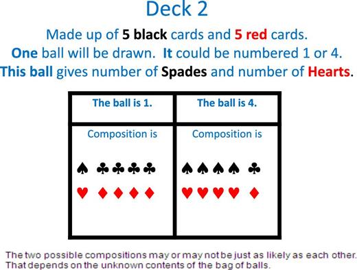
Deck 2 (1-ball condition).
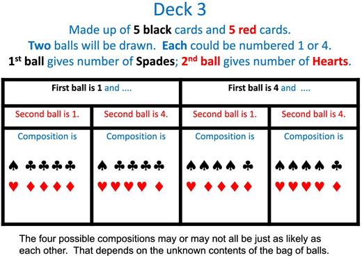
Deck 3 (2-ball condition).
Several features of these procedures are worth stressing. As just explained, in both conditions, subjects were told that the compositions of decks 2 and 3 would be determined by drawing the appropriate number of balls from the opaque bag, but they were not told anything more than this about the contents of the opaque bag except that it contained balls of which some were numbered 1 and the others numbered 4. Since subjects did not know the relative frequency of the types of ball in the bag, they had no objective probabilities for the possible compositions of either deck 2 or deck 3. Thus, for acts resolved with these decks, subjects faced genuine ambiguity, not two-stage objective lotteries. Indeed, the first stage of resolution of uncertainty (i.e., determination of the composition of decks 2 and 3) was ambiguous in just the same way as is a draw from an Ellsbergian urn containing specified types of objects in unspecified proportions.14
As the process determining the outcome of any given ambiguous act was conducted publicly, subjects were able to verify their limited information about it: balls were drawn from the opaque bag as described; they were numbered 1 or 4; and each of decks 2 and 3 was constructed to have the composition specified for that deck by the relevant slide, given the draws from the opaque bag. As long as subjects attended to what they were told and realized we would not make statements about procedures that would be publicly exposed as false later in the session, we are justified in assuming that the subjects believed that each deck would have one of the compositions we had stated to be possible for it.
Some authors, such as Charness et al. (2013), conjecture that subjects of previous experiments may have suspected that devices used to resolve ambiguity might be stacked against them by the experimenters. Our design is structured so that, as long as subjects believed information that they would be able to verify, such suspicions would be minimized, and so that any remaining ones would not undermine our objectives. Some subjects may have considered the possibility that, when filling the opaque bag before the session, we might work against their interests but, provided they remained subjectively uncertain of the content of the opaque bag (e.g., because of also considering other scenarios about our characters), the required ambiguity would have remained.15
Although subjects had no information about the relative likelihoods of the two possible compositions of deck 2, nor about those of the first and fourth possible compositions of deck 3 (relative either to each other or the other two compositions), the information given to subjects implied that the second and third possible compositions of deck 3 were equally likely. (As draws from the opaque bag were with replacement, 1 followed by 4 was precisely as likely as 4 followed by 1.) This is significant in relation to Section 2.2 as it means that a subject who understood the implications of what they were told would attach equal weight to possible compositions of deck 3 corresponding to p2 and p3. Of course, we cannot be sure that all subjects appreciated this. Nevertheless, the information that they were given was entirely symmetric between the second and third possible compositions of deck 3, so even a subject who did not see that their information implied an equal likelihood of those compositions would have been given no grounds for thinking either of them more or less likely than the other. In view of these points, we start from a maintained hypothesis that subjects did weight the second and third possible compositions of deck 3 equally, as well as believing the possible compositions of each deck to be those we had stated to be possible for it. We discuss the robustness of our conclusions with respect to violations of this maintained hypothesis in Appendix A.
Finally, the 2-ball condition is not just a device for giving subjects a reason to put equal weight on the second and third possible compositions of deck 3. It also implements the key feature of the theoretical framework of Section 2.2 that the DM understands that the uncertainties about the “B-component” (here, the relative frequency of spades and clubs) and uncertainties about the “R-component” (here, the relative frequency of hearts and diamonds) are resolved separately. This would not have been achieved by an (arguably more classically Ellsbergian) design in which the four possible compositions of deck 3 were simply listed for subjects.
3.4. Elicitation of Preferences
Our procedure for inferring a preference between two acts was to elicit a certainty-equivalent for each of them and to infer the binary preference from the relative magnitudes of the certainty-equivalents. This procedure allows incentivized elicitation of indifference between two acts while avoiding the problems of choice tasks in which subjects are allowed to express indifference directly.16 To infer a subject's certainty-equivalent of a given act, we used a form of choice-list procedure that yielded interval estimates with a bandwidth of €0.05. The procedure is similar to that of Tversky and Kahneman (1992), sharing with it the important feature that, because estimated certainty equivalents are obtained from choices, they should be unaffected by endowment effects.
In our case, the details of this procedure were as follows. Acts were displayed to subjects and choice lists completed by them on computers. The experiment was programed using z-Tree (Fischbacher 2007). Each choice list consisted of a table, each row of which described a choice between an act and a certain sum of money. Comparing successive rows of a given choice list, the sums of money rose moving down the table, but the act remained the same.17 In a basic list, the first row was a choice between the relevant act and €0; the certain sum of money then rose by €1 per row, till the final row was a choice between the act and €20. (See the Online Appendix for an example basic list.) As, for each act in our design, the two possible final outcomes were €20 and €0, we obviously expected subjects to choose the act in some early rows (at least the first one), to switch to the certainty in some subsequent row, and then to choose the certainty in all the remaining rows. After completing all rows of a basic choice list to their satisfaction, subjects had to confirm their choices; the computer would only accept confirmed responses with the single-switch property just described (or with no switches). After confirmation of their responses to a basic choice list, a subject who had switched proceeded to a zoomed-in list for the same act. This had the same structure as the basic one, except that (i) the first and last rows were, respectively, the two choices where the subject had switched from the act to the certainty in the basic list, with the responses to these rows filled in as the subject had already confirmed them; and (ii) across the intervening rows the certain sums of money rose in increments of €0.05. Again, the subject was required to choose between the act and each certain sum, observing the single switch requirement (and could adjust their responses until they confirmed them). A subject's certainty-equivalent was coded as the average of the certain sums in the last row of the zoomed-in list in which she chose the act and the first row in which she chose the certain sum.
3.5. Incentives
Each subject completed basic lists for ten acts, plus the corresponding zoomed-in lists. They were told at the start that, after they had completed all choices in all choice lists, one such choice would be selected at random to be for real18: that is, if they had chosen the certain sum of money in it, they would receive that sum and, if they had chosen the act, they would receive the outcome of its resolution.19 This is a form of the random lottery incentive system, widely used in individual choice experiments. It prevents confounding income effects between tasks that might arise if more than one task was paid (likewise, Thaler and Johnson’s (1990) “house money” effects). It is easy for subjects to understand and, in the current context, allows us to elicit certainty-equivalents without using cognitively more demanding devices such as auctions or forms of the Becker–De Groot–Marschak mechanism (Becker et al. 1964) in which buying or selling “prices” are declared and compared with randomly drawn ones.20
3.6. Sequence of Tasks
After the choice lists for the risky acts to be resolved with deck 1, subjects completed choice lists for the ambiguous acts f1, f2, and mix in the 1-ball condition (deck 2), followed by choice lists for the ambiguous acts f1, f2, mix, g1, and g2 in the 2-ball condition (deck 3). This progression from a risky environment to environments with progressively more complex ambiguity provided a natural sequence, conducive to subjects’ understanding.
Our design was constructed to make it “easy” for subjects to express indifference between the acts f1, f2, and mix. In each condition, all the basic choice lists for these three acts were shown and completed side by side on the same screen and subjects then proceeded to the corresponding zoomed-in lists, again with the lists for the three acts side by side on the same screen. As subjects could adjust their responses at any time until they confirmed them, they could easily align (or disalign) their certainty-equivalents for the acts appearing on the same screen.
After subjects had completed all choice lists for the mixed act and its constituents in the 1-ball condition and then in the 2-ball condition, they proceeded to a further screen with the basic choice lists for g1 and g2. They were completed side by side on the same screen, as were the corresponding zoomed-in lists. As the certainty-equivalents for these acts would be used to categorize subjects by ambiguity attitude (as we explain in the next section), we decided to elicit them last to rule out any possibility that subjects could construct their other choices deliberately to make them consistent with these ones. Subjects did not see these acts at all until after they had completed all tasks involving mix and its constituents in the 2-ball condition. The full experimental instructions are given in the Online Appendix.
3.7. Classification of Subjects
As it was resolved with deck 3, Table 4 and Figure 2 show that g1 offered 5 chances (out of 10) of a 50–50 die roll under every possible composition of the deck. In contrast, g2 would yield the die roll if a club or a heart was drawn; and the combined number of clubs and hearts was uncertain. Specifically, g2 offered 5, 8, 2, and 5 chances (out of 10), respectively, of the 50–50 die roll under the four possible compositions of deck 3. As the second and third possible compositions of that deck are equally likely, ambiguity aversion requires preference for g1 over g2 and ambiguity seeking the reverse preference. We use this fact to classify subjects by ambiguity attitude. Subjects who were indifferent between g1 and g2 were classified as ambiguity neutral, and all of the remainder as ambiguity sensitive, with the latter group divided into ambiguity seeking and ambiguity averse. Since the predictions in relation to preference over g1 and g2 are common to the smooth ambiguity and α-MEU models, this procedure is in line with and neutral between both models.
A potential qualification to this procedure is that, strictly, preference over g1 and g2 only determines a subject's attitude to ambiguity when the subject weights the second and third possible compositions of deck 3 equally. We review the robustness of our findings to violation of this condition and to other variations on our classification procedure in Appendix A.
3.8. Predictions and Control
We now put the theoretical predictions in the context of the design. For the 2-ball condition, which matches the setup of Section 2.2, the smooth ambiguity model predicts that those subjects who prefer g1 to g2 (ambiguity averse) should also prefer mix to each of f1 and f2; those who prefer g2 to g1 (ambiguity seekers) should also prefer each of f1 and f2 to mix; and those who are indifferent between g1 and g2 (ambiguity neutral) should be indifferent between mix, f1, and f2. In contrast, the α-MEU model predicts that all subjects should be indifferent in the 2-ball condition between mix and each of its constituents, regardless of their preference over g1 and g2.
We use the 1-ball condition as a control in several related ways. In the 1-ball condition, the smooth ambiguity model joins the α-MEU model in predicting indifference between f1, f2, and mix as, in each possible composition of deck 2, the number of spades equals the number of hearts, making the overall chances of receiving €20 the same under those three acts. If we observe preference for mix over its constituents among ambiguity-averse subjects in the 2-ball condition, and if the smooth ambiguity model correctly diagnoses the only source of that preference, the preference should be absent in the 1-ball condition. However, it is possible that subjects will be attracted (or repelled) by the mixed act relative to its constituent acts for reasons other than the hedging argument of the smooth ambiguity model. For example, subjects might have an attitude, positive or negative, towards the presence in the resolution of the mixed act of another source of uncertainty, die rolling, in addition to the drawing of cards from decks. But, if so, this should show up in both the 2-ball and 1-ball conditions. Thus, the difference between the two conditions is of particular interest, regardless of whether we observe the predicted indifference in the 1-ball condition.
To build on these points, we now define variables used in our data analysis. We use CE(f, C) to denote the certainty equivalent of act f in condition C (though we omit the condition where obvious from the context) and we use AvCE(f, g, C) to denote the (arithmetic) mean of a subject's certainty-equivalents for acts f and g in condition C. The following premium variables can then be defined for each subject:
| Mixed act premium (2-ball) | = | CE(mix, 2-ball) – AvCE(f1, f2, 2-ball); |
| Mixed act premium (1-ball) | = | CE(mix,1-ball) – AvCE(f1, f2, 1-ball); |
| 2-ball premium | = | CE(mix, 2-ball) – CE(mix, 1-ball); |
| Difference between mixed act premia | = | Mixed act premium (2-ball) – Mixed act |
| premium (1-ball). |
“Mixed act premium (2-ball)” measures the excess attractiveness of mix over its constituents in the condition where the smooth ambiguity model makes its distinctive prediction that ambiguity-averse subjects prefer the mixed act and ambiguity seekers the constituent acts.21 “Mixed act premium (1-ball)” measures the corresponding excess attractiveness in the condition where both models predict that all three types are indifferent between mix and its constituents. The variable “difference between mixed act premia” measures how far “excess attractiveness” of mix over its constituents is greater in the 2-ball condition than it is in the 1-ball condition. Thus, it measures the influence of the hedging of independent ambiguities consideration, controlling for any other factors that (contrary to both models being considered) may make mix either more or less attractive than its constituent acts in the 1-ball condition. Finally, the 2-ball premium measures directly the extent to which mix is more attractive when it does offer a hedge across independent ambiguities than when it does not.
According to the smooth ambiguity model, all of these premium variables should be positive for the ambiguity averse, zero for the ambiguity neutral, and negative for the ambiguity seeking, except for the mixed act premium (1-ball), which should be zero for all three types. The predictions of the α-MEU model are simply that each of the four premium variables should be zero for all types. Finally, SEU theory implies ambiguity neutrality and zero values of all four premium variables.22 Thus, three of the premium variables discriminate between models (for ambiguity-sensitive subjects): mixed act premium (2-ball), 2-ball premium, and difference between mixed act premia. The first is a direct comparison of the mixed act and its constituents in the 2-ball condition; the other two make comparisons across conditions, so exploiting the 1-ball control. The difference between mixed act premia is our most refined discriminator between the smooth ambiguity and α-MEU models: it measures the contribution of the hedging of the separately resolving ambiguities motive to preference over mix and its constituents, while controlling for other motives that might also affect that preference.
4. Results
4.1. Preliminaries
The experiment was conducted at the University of Tilburg. Ninety-seven subjects took part, all of whom were students of the university.23 They were paid a show-up fee of €5 on top of their earnings from the tasks, yielding a total average payment of €15.74. The main function of the risky acts resolved with deck 1 was to enhance subjects’ understanding of subsequent ones, but we report that the median certainty equivalents for 70% and 30% chances, respectively, of €20 were €11.73 and €5.58, suggesting levels of risk aversion not uncommon among experimental subjects. We now turn to ambiguous acts.
4.2. Results on Classification of Subjects
Certainty equivalents for g1 and g2 allow us to categorize subjects into three types: the ambiguity averse (CE(g1) > CE(g2)); the ambiguity neutral (CE(g1) = CE(g2)); and the ambiguity seeking (CE(g1) < CE(g2)). Out of a total of 97, the numbers of subjects of each type were 31, 50, and 16, respectively.
Although some studies have found a higher proportion of ambiguity-sensitive subjects than we do, Ahn et al. (2014, p. 206) found that 72.7% of their subjects were either ambiguity neutral or close to it and Charness et al. (2013, p. 3) found 60.3% of theirs to be ambiguity neutral. Thus, our findings are not out of line with the range of previous findings. Recall that our design was constructed to make it “easy” to reveal indifference between certain sets of acts the certainty equivalents of which were elicited side by side on the same screen. A subject who saw a relationship between two such acts that she regarded as making them equally attractive would have had no difficulty in giving certainty-equivalents that reflected that judgment. From this perspective, the proportion of subjects coded as ambiguity neutral is actually quite encouraging, even though it lowers the proportion coded as ambiguity sensitive. As subjects clearly were able to express indifference between g1 and g2, there is no reason to think they would not have been able to do so between mix and its constituents (the certainty equivalents of which were also elicited side by side on the same screen) if they saw fit.24
Notwithstanding ambiguity neutral being the largest group, the mean difference CE(g1) − CE(g2) was €0.45 across all subjects, reflecting some ambiguity aversion on average. The corresponding figures for the two ambiguity-sensitive types were €1.90 for the ambiguity averse and –€0.93 for the ambiguity seeking.
4.3. Comparing Certainty Equivalents: Central Tendencies
As an initial display of our findings, Figure 3 reports the mean certainty equivalents, for each ambiguous act under each condition, separately by type of subject.
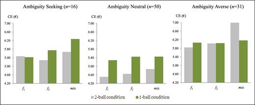
Mean CEs for ambiguity-seeking, ambiguity-neutral, and ambiguity-averse subjects.
As explained in Section 3.8, the most important features of our data are the premium variables defined in terms of the certainty equivalents. The mean, median, and standard deviations (SDs) of each of the four premium variables are reported Table 5.25
Premia (in €, rounded to nearest cent).
| Ambiguity seeking (n = 16) | Ambiguity neutral (n = 50) | Ambiguity averse (n = 31) | |||||||
|---|---|---|---|---|---|---|---|---|---|
| Mean | Median | SD | Mean | Median | SD | Mean | Median | SD | |
| Premia | |||||||||
| Mixed act (2-ball) | 0.30 | 0.46 | 2.68 | 0.29 | 0.00 | 1.58 | 1.06 | 0.73 | 2.63 |
| Mixed act (1-ball) | 0.69 | 0.00 | 2.53 | 0.09 | 0.00 | 2.02 | 0.12 | 0.00 | 2.39 |
| 2-ball | –0.60 | –0.43 | 1.85 | –0.58 | 0.00 | 2.13 | 0.83 | 0.55 | 2.53 |
| Difference between mixed act premia | –0.39 | –0.64 | 2.01 | 0.21 | 0.00 | 2.00 | 0.95 | 0.30 | 2.39 |
Several points stand out from Figure 3 and Table 5. If, first, we confine attention to subjects coded as ambiguity averse, then the findings are, at eyeball level, very much in line with the predictions of the smooth ambiguity model. In particular, the right-hand panel of Figure 3 shows that, for these subjects, mix seems to have been judged on average to be notably more attractive than its constituents in the 2-ball condition, but not in the 1-ball condition. Table 5 indicates that, for the ambiguity averse, the mixed act premium (2-ball) and the 2-ball premium are both, on average and by median, positive and seemingly nontrivial, whereas the central tendencies of the mixed act premium (1-ball) are close to zero.26
For ambiguity-averse subjects, Wilcoxon signed-rank tests reveal that CE(mix, 2-ball) exceeds each of CE(f1, 2-ball) and CE(f2, 2-ball) (p = 0.006 and p = 0.008, respectively) and also that CE(mix, 2-ball) is larger than CE(mix, 1-ball) (p = 0.035). In contrast, we cannot reject equality of CE(mix, 1-ball) with either CE(f1, 1-ball) or CE(f2, 1-ball) (p = 0.664 and p = 0.635, respectively). Thus, there is evidence, at the level of central tendencies, in favor of the hypothesis that ambiguity-averse subjects value the hedge against independent ambiguities that mix offers over its constituents in the 2-ball condition but that, as also predicted by the smooth ambiguity model, this attraction to mix disappears in the 1-ball condition, where the ambiguities are not independent.
In the case of subjects coded as ambiguity neutral, all theories agree. The medians of each of the premium variables are exactly as predicted by the theories. However, surprisingly, ambiguity-neutral subjects seem from Figure 3 to prefer each of the acts in the 1-ball condition over the same act in the 2-ball condition, as Wilcoxon signed-rank tests confirm.27 The reason for this is unclear but, one possibility is that some subjects are averse to greater numbers of possible compositions of the deck. Whatever the reason, as the effect favors the 1-ball version, it does not seem to indicate any factor that would contribute to our earlier finding that ambiguity-averse subjects prefer the 2-ball version of mix over its constituents. Indeed, if anything, it strengthens that finding.
Our findings for subjects coded as ambiguity seeking are more mixed than those for the ambiguity averse. For example, for these subjects, the mean and median values of the mixed act premium (2-ball) both have the wrong sign from the perspective of the smooth ambiguity model. However, the picture changes if we consider the premium variables that use the 1-ball control. The means and medians of the 2-ball premium and the difference between mixed act premia all take the sign predicted by the smooth model. That said, these effects receive only very limited corroboration in statistical tests,28 so we cannot reject the predictions of the α-MEU model for ambiguity-seeking subjects. Given the small number of such subjects, it would inevitably be difficult to detect any statistically reliable pattern in their behavior.
However, ambiguity-averse and ambiguity-seeking categories can be pooled, using transformations of the three premium variables that discriminate between models in predictions for ambiguity-sensitive subjects. For each of these variables, the transformation makes deviations from zero in the direction predicted by the smooth ambiguity model positive, and deviations in the opposite direction negative, by multiplying the original premium variable by −1 for the ambiguity seeking (only). Then, the smooth model predicts a positive value of the transformed variable for any ambiguity-sensitive subject, whereas the α-MEU model predicts a zero value, and a negative value is possible but not predicted by either model. This transformation allows statistical tests to be conducted on the n = 47 ambiguity-sensitive subjects taken as a single group. We find that the transformed mixed act premium (2-ball) is only marginally significantly larger than zero (p = 0.061), but the transformed 2-ball premium and transformed difference in mixed act premia are both significantly larger than zero (p = 0.013 and p = 0.012, respectively), so that, again, exploiting the 1-ball control sharpens the picture.
4.4. Categorical Analysis
The analysis of the previous subsection is subject to two limitations. First, it concentrates on magnitudes of certainty equivalents and premium variables, whereas the theoretical predictions are really about ordinal comparisons of certainty equivalents (and hence only about signs of the premium variables). Secondly, as it focuses on the “typical” subject in each type, it does not fully capture the proportion of subjects in a given type conforming to a given prediction. In this subsection, we present a brief categorical analysis that addresses these points.
We define (with slight abuse of terminology) the sign of a variable as taking one of three values: strictly positive, zero, or strictly negative. Table 6 presents contingency tables for the sign of CE(g1) − CE(g2) (i.e., the subject's type) against the sign of each of the three premium variables that discriminate between models. The table gives the frequencies of subjects with each combination of type and sign of premium variable, for each premium variable. The first number in each cell gives the absolute number, for each frequency.
“Signs” of premia and ambiguity attitude.
| CE(g1) − CE(g2) | ||||
|---|---|---|---|---|
| Ambiguity attitude | ||||
| <0 (Seeking) | 0 (Neutral) | >0 (Averse) | ||
| Mixed act premium (2-ball) | >0 | 9 | 13 | 21 |
| 0 | 1 | 26 | 3 | |
| <0 | 6 | 11 | 7 | |
| 2-ball premium | >0 | 4 (4) | 12 (7) | 19 (17) |
| 0 | 0 (4) | 15 (23) | 2 (6) | |
| <0 | 12 (8) | 23 (20) | 10 (8) | |
| Difference between mixed act premia | >0 | 5 (5) | 16 (16) | 19 (17) |
| 0 | 1 (1) | 19 (21) | 4 (7) | |
| <0 | 10 (10) | 15 (13) | 8 (7) | |
As it may be difficult for a subject to achieve a value of precisely zero for a given premium variable, we also consider an alternative coding. We have already argued that subjects seemed to have no difficulty in achieving CE(g1) = CE(g2), as these two certainty equivalents were elicited side by side on the same screen. For this reason, we use a requirement of exact equality here when classifying subjects as ambiguity neutral. But, that argument is less compelling for some of the premia. To achieve either a 2-ball premium of zero or a difference between mixed act premia of zero requires suitable alignment of certainty-equivalents elicited across different screens. In view of these points, Table 6 also indicates parenthetically, for these variables, the frequencies under a revised coding scheme in which a sign of zero is attributed to the premium variable if its absolute value is no more than €0.20 from zero (an allowance equivalent to four rows of a zoomed-in choice -list). Unsurprisingly, this pulls more observations into the central rows of the relevant panels of Table 6.
According to the smooth ambiguity model, each subject's type should match the sign of their premium variable, for each of the three premium variables presented in Table 6. To capture the extent of conformity with this prediction, we calculate, for each of these premium variables, the sign-matching rate, defined as the percentage of subjects for whom the type matches the sign of the premium variable. Correspondingly, for each premium variable, we also calculate the sign-zero rate, defined as the percentage of subjects for whom the sign of the premium variable is coded as 0, in accordance with the α-MEU model.
Table 7 reports both rates, for each of the premium variables from Table 6, separately for all subjects, ambiguity-sensitive subjects, and ambiguity-averse subjects. Rates are given to the nearest percentage. As with Table 6, unparenthesized entries correspond to the stricter coding rule for a zero sign on the premium variable and parenthesized entries to the looser coding. By construction, the looser coding rule for a sign of zero on the premium variable cannot lower the sign-zero rate. In fact, as Table 7 shows, it raises that rate in all cases and in some cases substantially so. In contrast, the looser coding rule sometimes raises and sometimes lowers the sign-matching rate, and most of these adjustments are quite small. In terms of the comparative performance of the smooth ambiguity and α-MEU models for a given premium variable and group of subjects, what matters is the difference between the sign-matching and the sign-zero rate. This is reduced by the looser coding rule for the latter rate in all cases shown.
Sign-matching and sign-zero rates (%) by premium variable.
| Premium variable | Rate: Sign-… | All (n = 97) | Ambiguity sensitive (n = 47) | Ambiguity averse (n = 31) |
|---|---|---|---|---|
| Mixed act (2-ball) | Matching | 55 | 57 | 68 |
| Zero | 31 | 9 | 10 | |
| 2-ball | Matching | 47 (49) | 66 (53) | 61 (55) |
| Zero | 18 (34) | 4 (21) | 6 (19) | |
| Difference between | Matching | 49 (49) | 62 (57) | 61 (55) |
| mixed act premia | Zero | 25 (30) | 11 (17) | 13 (23) |
Using the looser of our codings where applicable, the sign-matching rate exceeds the sign-zero rate in every case reported in Table 7, by a margin never lower than 15 percentage points. If attention is restricted to ambiguity-sensitive subjects, then, using the coding that favors the sign-zero rate in the second and third cases, the sign-matching rate exceeds it by 48 (= 57–9) percentage points, 32 (= 53−21) percentage points, and 40 (= 57–17) percentage points for the mixed-act premium (2-ball), the 2-ball premium, and the difference between mixed act premia, respectively. In this respect, the smooth ambiguity model outperforms the α-MEU model.
That said, the performance of the smooth ambiguity model in Table 7 is far from perfect. The sign-matching rates reported in the “All” column are only around 50%, and none of those reported in other columns exceed 68%. (These figures compare with a benchmark of 33%, if the three values of sign were allocated at random.)
4.5. Main Experiment: Summary of Findings
The analysis of central tendencies reported in Section 4.3 and the individual-level categorical analysis of Section 4.4 broadly cohere with one another.
Where the smooth ambiguity and α-MEU models agree in relation to our design—that is, in their predictions for the ambiguity neutral in the 2-ball condition and for all types in the 1-ball condition—their shared predictions perform well, as judged by central tendencies, but less well at the individual level. For example, the median value of each of our premium variables is zero in every case where both models predict that it will be zero, but neither model accounts for the fairly frequent incidence (evidenced by the central data column of Table 6) of individual-level violations of the shared prediction that each premium variable will be zero for each ambiguity-neutral subject.
Our potential for discriminating between models is provided by ambiguity-sensitive subjects, be they ambiguity averse or ambiguity seeking, since the two models disagree in their predictions for these subjects. Too few subjects are coded as ambiguity seeking for a statistically significant pattern to emerge when that group is considered on its own but when all ambiguity-sensitive subjects are pooled, the three premium variables that distinguish between models tell broadly in favor of the smooth ambiguity model. This generalization holds for individual-level analysis and central tendencies alike, but the evidence for it is less clear for the premium variable that only draws information from the 2-ball condition than it is for the two premium variables that exploit our 1-ball control by drawing information from both conditions. This qualification suggests that neither model fully captures the behaviour of the whole set of ambiguity-sensitive subjects in either condition taken separately, yet comparison of the 2-ball and 1-ball conditions is still broadly consistent with responses to separately resolving ambiguities in directions predicted by the smooth ambiguity model.
The qualification about reliance on measures that exploit the 1-ball control is not needed when attention is restricted to subjects coded as ambiguity averse as, for these subjects, all of the three premium variables that discriminate between models tell essentially the same story in both forms of analysis. We find clear and statistically significant patterns in the behavior of the subjects coded as ambiguity averse that conform more closely to the predictions of the smooth ambiguity model than to those of the α-MEU model.
5. Extensions
Before concluding, we comment on some extensions of our investigations reported in this section and, especially, in Appendices A to C.
5.1. Robustness to Categorization
As noted in Section 3.7, our categorization of subjects by ambiguity attitude assumes that they see the second and third compositions of deck 3 as equally likely, as implied by the information provided. It also assumes that, even when they have this belief, they reveal ambiguity neutrality through exact equality between CE(g1) and CE(g2). Appendix A explores the robustness of our conclusions to relaxation of these assumptions: Appendix A.1 considers the possibility of subjects not realizing that the second and third compositions of deck 3 are equally likely and Appendix A.2 what happens if we allow closeness (rather than only equality) between CE(g1) and CE(g2) to count as indicating ambiguity neutrality. In each case, the details of our findings are affected but the general tenor is not.
A different possible concern about our analysis, in view of the findings of previous experiments in the literature, is its reliance on expected utility theory as the model of choice under objective risk. In this respect, our analysis is true to the smooth and α-MEU models, as usually formulated.29 Notwithstanding this, in Appendix B, we show that our theoretical analysis would be robust to a reformulation of these models in which expected utility theory is replaced in this role by any one of a range of nonexpected utility models.
5.2. Divide Across Models: Theory and a Follow-up Experiment
In Appendix C, we substantiate the assertion of Section 1 that the α-MEU and smooth ambiguity models stand as examples of broader classes of models of ambiguity-sensitive preference: that is, respectively, of models of preferences whose representations focus exclusively on minimum and/or maximum expected utilities and of models whose representations also give weight to nonextremal expected utilities. In particular, we identify other models that, under important but plausible assumptions, share the predictions of models that we have considered in the main text in the context of our design.
In the case of the main study reported above, one model—that of Seo (2009)—shares the predictions of KMM’s smooth ambiguity model in a particularly direct way. But, as footnote 7 explains, the two models differ in subtle respects, in particular in tying or not tying ambiguity aversion to violation of ROCL. This issue connects to an important debate in the ambiguity literature about whether sensitivity towards ambiguity is simply the result of nonstandard reduction of compound lotteries. The experimental data of Halevy (2007) suggest that this is the case:30 ambiguity aversion is strongly associated with violations of ROCL. Abdellaoui et al. (2015), however, observe that ambiguity-neutral subjects also often violate ROCL and that a significant proportion of subjects who do reduce compound lotteries are sensitive towards ambiguity, suggesting that ambiguity attitude is more than DMs violating ROCL.
In view of these points, we ran an additional experiment with two-stage objective lotteries in place of the ambiguous acts of the main study. In this follow-up study, the objective probabilities of the possible compositions of decks 2 and 3 respectively were given to subjects. Specifically, the opaque bag that determined the composition of deck 2 and deck 3 was publicly filled with an equal number of balls numbered 1 and 4, so that subjects knew that each possible composition of deck 2 was equally likely, as was each possible composition of deck 3. In all other respects, the new treatment was identical to the main experiment.31 Since the probabilities for each possible composition are objectively given, in the new experiment the behavior implied by MEU and KMM’s model are identical and consistent with that implied by expected utility. As noted in footnote 7, in Seo's (2009) model, violation of ROCL is implied by a concave |$\phi$| and unaffected by whether the second-order uncertainty is an objective risk or not.
In total, 86 undergraduate students (average payment €15.24) from Tilburg University participated.32 Classifying subjects based on the difference between the certainty-equivalent of acts g1 and g2 yields the same general pattern of preferences as in the main experiment. In particular, 20 subjects reported CE(g1) > CE(g2), 16 reported CE(g1) < CE(g2), and 50 reported CE(g1) = CE(g2). As all risks are objective in the follow-up experiment, the two strict inequalities are violations of ROCL and, in that sense, contrary to KMM’s model and MEU. A two-sided Wilcoxon rank-sum test does not reveal a statistically significant difference between the two experiments in the statistic CE(g1) − CE(g2) (p = 0.236). These findings are in line with the Seo (2009) model and also suggestive of the findings of Halevy (2007).
Just as with the main experiment, it is particularly interesting to consider the preferences over mix and its constituents of subjects appearing to be “ambiguity averse”, in the sense that (CE(g1) > CE(g2)).33 But, here the picture is mixed, in part depending on whether the 1-ball control is used. For subjects with CE(g1) > CE(g2) in the follow-up experiment, one-tailed Wilcoxon signed-rank tests provide some evidence that mix is preferred to its constituents, as CE(mix, 2-ball) exceeds each of CE(f1, 2-ball) and CE(f2, 2-ball) (p = 0.063 and p = 0.039, respectively). However, this evidence disappears when measures exploiting the 1-ball control are used. In particular, the 2-ball premium is not significantly positive (p = 0.383) and nor is the difference between mixed act premia (p = 0.470). Recall in contrast that, in the main experiment, all premium variables told the same story for the ambiguity averse. This difference between the findings of the two experiments is more supportive of KMM’s version of the smooth model than of that of Seo (2009).
Moreover, in the follow-up experiment, a Friedman test does not detect differences between the distributions of the ranks of the certainty equivalents of the acts f1, f2, and mix in the 1-ball condition, f1, f2, and mix in the 2-ball condition, and g1 and g2 in the 2-ball condition (p = 0.658). In contrast, a similar Friedman test for the main experiment reveals that the ranks of those certainty equivalents are different (p = 0.012). These findings suggest that the aggregate pattern of preference over these acts that we observe in the main experiment is not entirely driven by violations of ROCL in preferences over objective lotteries. However, two qualifications are in order. First, we do observe many violations of ROCL at the individual level in the follow-up experiment, so its findings do not in themselves support ROCL for objective risks. Secondly, as the follow-up study was run later than the main one, subjects were not randomly assigned between the two; so, any comparison of the studies must be made with caution. Partly for this reason, we focus on the main study in our final concluding comments.
6. Concluding Remarks
We have presented an experiment designed to discriminate empirically between two well-known and widely applied models of ambiguity attitude—the α-MEU and smooth ambiguity models—which stand as representatives of a broader theoretical divide. This is important as the conclusions of existing applied economic models that incorporate ambiguity are often derived from specific models of ambiguity sensitivity, sometimes on one side of the divide we mark and sometimes on the other.
Our strategy for distinguishing between models focuses on whether or not an agent's preference for hedging separate ambiguities depends on ambiguity attitude. Interpreting our findings narrowly in terms of a comparison of the smooth ambiguity and α-MEU models, we find that, although neither model captures all aspects of our data, there are striking features of the data that conform more closely to the smooth ambiguity model than to the α-MEU model. As explained in Section 1 and Appendix C, this discrimination extends to a broader divide between models that do or do not give weight to nonextreme expected utilities, among those considered possible.
Finally, our results provide a more general reassurance to the theories of ambiguity aversion. It has long been argued, at a theoretical level, that reliance on stochastic mixing as a way to hedge ambiguity is a defining part of a rational response to ambiguity. Indeed, such is the motivating basis of Schmeidler's (1989) Uncertainty Aversion axiom, which lies at the heart of ambiguity-averse preference models, quite generally (Cerreia-Vioglio et al. 2011). However, the best-known prior study that we are aware of which investigates the link between ambiguity aversion and preference for randomization—Dominiak and Schnedler (2011)—reports little support for this central premise of theories of ambiguity aversion. In view of this, it is particularly notable that our main finding, specifically strict preference for mix over f1 and f2 on the part of the ambiguity averse in the 2-ball condition, supports the Uncertainty Aversion axiom.34 Hence, a further overall takeaway from our findings is that they provide evidence for a link between ambiguity aversion and propensity to use randomization to hedge ambiguity, and thus for the central foundational principle of theories of ambiguity aversion, quite generally.
Appendix A: Robustness to Classification
In this appendix, we consider the robustness of our findings to variations in our procedure for classifying subjects by ambiguity attitude, as explained in Section 5.
A.1. Robustness Towards Beliefs
As explained in Section 3.7, our classification of subjects as ambiguity averse, ambiguity neutral, or ambiguity seeking used a procedure that, strictly, relies on subjects being indifferent, in the 2-ball condition, between f1 and f2. In fact, for 71 subjects, the condition CE(f1, 2-ball) = CE(f2, 2-ball) holds exactly. For the remaining 26 subjects, the statistic CE(g1) − CE(g2) is well defined, but no longer sufficient to identify a subject's ambiguity attitude, as the subjects do not appear to weight the second and third possible compositions of deck 3 equally. In this appendix, we comment on how that affects our analysis, in particular, the robustness of our conclusions regarding the comparison of models.
For purposes of this discussion, we fix the domain of preferences to include those described by:
an α-MEU model with the set of probabilities in the representation given by |$\mathcal{P}$| = {pi | i = 1, …, 4}, or its convex hull, where pi refers to the probabilities described in Table 2;
an SEU model (specifically, an Anscombe–Aumann model) that puts positive weight on each of the four probabilities, pi, i = 1, …, 4;
a smooth ambiguity model with a nonlinear |$\phi$| and a μ that puts positive weight on each of the four probabilities, pi, i = 1, …, 4.
Within this domain, the α-MEU model predicts indifference between f1 and f2 and mix regardless of preference over g1 and g2. In contrast, both the smooth ambiguity and SEU models allow nonindifference between f1 and f2 if p2 and p3 are weighted unequally.35 Importantly, they also require that the directions of a subject's preference over g1 and g2 and her preference over mix and f2 match, as can seen from an inspection of the relevant rows of Table 3. However, SEU imposes an additional restriction that the smooth model does not, namely, that the direction of preference between f1 and f2 must also match that between g1 and g2. Under the smooth ambiguity model, nonlinearity of |$\phi$| could upset this correspondence, thereby distinguishing SEU from smooth ambiguity. In fact, of the 26 subjects who are not indifferent between f1 and f2 in the 2-ball condition, only 5 conform to the additional restriction imposed by SEU.
Thus, if we set SEU aside and focus on the two models of ambiguity sensitivity, we may use a comparison of the preferences between mix and f2 and between g1 and g2 as a means of discriminating between the models, even when the subject is not indifferent between f1 and f2. Hence, our strategy for comparing the α-MEU and smooth ambiguity models is a simple modification of our analysis in the main part of the paper. We replace AvCE(f1, f2, 2-ball) with CE(f2, 2-ball) in the definitions of mixed act premium (2-ball) and difference between mixed act premia. For a given sign of CE(g1)–CE(g2), the predictions of the smooth ambiguity model for the signs of the two redefined premium variables are exactly the same as for the original definitions. Similarly, for the α-MEU model, the implications for the signs of the two redefined premium variables are exactly as for the original definitions, since the model predicts indifference between mix and f2 for any value of CE(g1) − CE(g2). These points are unaffected by whether CE(g1) − CE(g2) indicates ambiguity attitude.
The redefinition can only affect subjects for whom CE(f1, 2-ball) ≠ CE(f2, 2-ball). (These subjects are spread roughly evenly across the three categories by the sign of CE(g1) − CE(g2).) The sign of the mixed act premium (2-ball) is changed by the redefinition in only nine cases and the sign of the difference between mixed act premia in only three. Clearly, the latter point makes little difference, so we focus on the former, using the stricter coding rule for a zero sign on a premium, because the redefinition of the mixed act premium (2-ball) makes it the difference of two certainty-equivalents elicited next to each other. For the mixed act premium (2-ball), the number of subjects with a zero sign rises from 30 to 35, whereas the number with a sign matching that of CE(g1) − CE(g2) falls from 53 to 51. Though this impact of the redefinition slightly favors the α-MEU model, the sign-matching rate for all subjects still exceeds the sign-zero rate by more than 16 percentage points. Thus, the main qualitative conclusions of the categorical analysis (Section 4.4) are not affected. Moving beyond signs, the median mixed act premium (2-ball) rises by 2 (resp. 0) euro cents among subjects with CE(g1) − CE(g2) > (resp. = ) 0. Hence, for these subjects the modification makes very little difference to the central tendency. But, among those with CE(g1) − CE(g2) < 0, the median mixed act premium (2-ball) rises from €0.46 to €0.85. This is a movement in the wrong direction for both the smooth and α-MEU models. In that sense, it does not affect the conclusions that we drew from our analysis of the central tendencies of certainty-equivalents in Section 4.3, about the relative performance of those models.
A.2. Robustness to Trembles
In Section 4, we used exact equality of CE(g1) and CE(g2) to classify subjects based on their attitude towards ambiguity, because these certainty equivalents were presented to subjects side by side on the same screen. Here we consider whether our results are robust if we apply looser coding rules to classify subjects in terms of ambiguity attitude. In particular, we distinguish between three coding rules for monetary sums. Under strict coding (S), a variable of interest has to be exactly zero in order to be counted as zero, whereas under Tremble-Tolerant (TT) coding, the variable of interest has to be no more than +0.05 and no less than −0.05, and under Loose (L) coding, it has to be no more than +0.20 and no less than −0.20. In terms of choice behavior, these codings translate respectively into no margin of error in a zoomed-in choice-list (S), a margin of error equivalent to one row of a zoomed-in choice list (TT), and a margin of error equivalent to four rows of a zoomed-in choice list (L), respectively.
Tables A.1 and A.2 replicate the results reported in Table 5, using Tremble-Tolerant and Loose coding, respectively, when classifying subjects by attitude towards ambiguity, rather than the Strict coding used in Table 5. By construction, applying a looser coding to type classification reduces the number of ambiguity-sensitive subjects, specifically in our case, from 47 under Strict coding (Table 5) to 39 under Tremble-Tolerant coding (Table A.1) and 36 under Loose coding (Table A.2). We have already defended Strict coding for use in identifying ambiguity neutrality, on the grounds that CE(g1) and CE(g2) are elicited right next to each other on the same screen. In view of this point, we also see Tremble-Tolerant as the more plausible of the two alternative coding rules for ambiguity attitude. But, we include both for completeness.
Premia (in €, rounded to nearest cent) with Tremble Tolerant coding.
| Ambiguity seeking (n = 11) | Ambiguity neutral (n = 58) | Ambiguity averse (n = 28) | |||||||
|---|---|---|---|---|---|---|---|---|---|
| Mean | Median | SD | Mean | Median | SD | Mean | Median | SD | |
| Premia | |||||||||
| Mixed act (2-ball) | 0.89 | 1.05 | 2.69 | 0.24 | 0.00 | 1.66 | 1.03 | 0.69 | 2.77 |
| Mixed act (1-ball) | 0.97 | 0.00 | 2.98 | 0.10 | 0.00 | 1.95 | 0.07 | 0.13 | 2.43 |
| 2-ball | –0.20 | –0.05 | 1.57 | –0.59 | –0.02 | 2.12 | 0.84 | 0.53 | 2.63 |
| Difference between mixed act premia | −0.09 | −0.70 | 1.65 | 0.13 | 0.00 | 2.06 | 0.95 | 0.29 | 2.46 |
Premia (in €, rounded to nearest cent) with Loose coding.
| Ambiguity seeking (n = 11) | Ambiguity neutral (n = 61) | Ambiguity averse (n = 25) | |||||||
|---|---|---|---|---|---|---|---|---|---|
| Mean | Median | SD | Mean | Median | SD | Mean | Median | SD | |
| Premia | |||||||||
| Mixed act (2-ball) | 0.89 | 1.05 | 2.69 | 0.36 | 0.00 | 1.73 | 0.82 | 0.50 | 2.84 |
| Mixed act (1-ball) | 0.97 | 0.00 | 2.98 | 0.05 | 0.00 | 2.00 | 0.19 | 0.25 | 2.39 |
| 2-ball | –0.20 | –0.05 | 1.57 | –0.45 | 0.00 | 2.18 | 0.66 | 0.10 | 2.70 |
| Difference between mixed act premia | –0.09 | –0.70 | 1.65 | 0.31 | 0.00 | 2.19 | 0.63 | 0.15 | 2.33 |
Our main findings regarding ambiguity-averse subjects replicate under the Tremble-Tolerant coding, despite the lower number of observations.36 First, the central tendencies of the premium variables are hardly affected by switching from Strict to Tremble-Tolerant coding. Moreover, the mixed act premium (2-ball) is again significantly positive (p = 0.019), whereas the mixed act premium (1-ball) is not (p = 0.328). The difference between these premia is also significantly positive (p = 0.044). Although, under Loose coding, the mixed act premium (2-ball) and mixed-act premium (1-ball) are lower than those under tighter codings and neither is significantly different from zero, this may in part be due to low power and, in any case, we see the Tremble-Tolerant coding as more plausible for classification of subjects by type of ambiguity attitude. Nevertheless, the reader may be surprised that reducing the number of subjects coded as ambiguity averse, by adopting Loose rather than Strict coding for ambiguity neutrality, lowers the mean and median of the key premium variables for ambiguity-averse subjects. It is important to note, however, that the predictions of the smooth ambiguity model for these variables are only ordinal. In particular, the model does not require that the larger is CE(g1) − CE(g2) the larger will be the premium variables predicted to be positive for the ambiguity averse. Instead, the predictions are about signs.
In view of this, we turn to the robustness of our categorical analysis. For this, we need to consider combinations of coding rules, as we must code both the type of ambiguity attitude and the sign of the premium. So, for brevity, we focus—for each premium variable analyzed in Section 4.4—on the robustness of our findings to different coding rule combinations of one measure of the comparative performance of the smooth ambiguity and α-MEU models, namely, the excess of the sign-matching rate over the sign-zero rate for ambiguity-sensitive subjects. Table A.3 reports this statistic for each premium variable considered in Section 4.4, for four different coding combinations.37 The label at the top of each column gives the coding combination that column reports, with the first word of the label giving the coding rule applied to ambiguity neutrality in the classification by type and the second word the coding rule applied in coding the sign of the premium. The third and fourth columns report new codings, not considered in the main text, whereas the first two columns repeat, for comparison, the two cases considered in Section 4.4 (where we insisted on Strict coding for type).
Sign-matching rate minus sign-zero rate (%) for ambiguity-sensitive subjects: different codings.
| Codinga | ||||
|---|---|---|---|---|
| Strict–Strict | Strict–Loose | TT–Loose | Loose–Loose | |
| (n = 47) | (n = 47) | (n = 39) | (n = 36) | |
| Mixed act premium (2-ball) | 49 | 38 | 31 | 25 |
| 2-ball premium | 62 | 32 | 31 | 25 |
| Difference between mixed act premia | 51 | 40 | 36 | 31 |
| Codinga | ||||
|---|---|---|---|---|
| Strict–Strict | Strict–Loose | TT–Loose | Loose–Loose | |
| (n = 47) | (n = 47) | (n = 39) | (n = 36) | |
| Mixed act premium (2-ball) | 49 | 38 | 31 | 25 |
| 2-ball premium | 62 | 32 | 31 | 25 |
| Difference between mixed act premia | 51 | 40 | 36 | 31 |
Notes: a. Strict–Strict refers to Strict coding of types and signs of premia; Strict–Loose refers to Strict coding of types and Loose coding of signs of premia; TT–Loose refers to Tremble Tolerant coding of types and Loose coding of signs of premia; Loose–Loose refers to Loose coding of types and signs of premia. Cell entries are rounded to the nearest integer.
As can be seen in Table A.3, our main result that the smooth model outperforms the α-MEU model for ambiguity-sensitive subjects is robust to the coding used, in the sense that in all cases shown the sign-matching rate exceeds the sign-zero rate by at least 25 percentage points. However, the result becomes less pronounced under looser coding as we move from left to right along any row of the table, with both sample size and the excess of the sign-matching rate over the sign-zero rate falling.
Appendix B: Nonexpected Utility for Risk
A possible concern about our theoretical analysis of preference over the acts is its use of expected utility theory as the underlying model of choice under risk. In this respect, our analysis is true to the smooth ambiguity and α-MEU models as usually formulated. But, as there is evidence from many experiments that subjects deviate from expected utility theory under risk (Starmer 2000), we might wonder how the theoretical analysis would be affected if this were true of our subjects too. It is possible to imagine more general formulations of these models that allow an induced probability distribution on consequences to be evaluated by a quite general nonexpected utility functional (see, e.g., the discussion of Corollary 1 in KMM). In this appendix, we show that our testing strategy for distinguishing between the α-MEU and the smooth ambiguity models, and our conclusions about the relative support of each model in the data, would be robust to such reformulation.
An act together with a given probability distribution on the state space induces a probability distribution on consequences. Since consequences may be lotteries, the induced distribution is, in general, a distribution over lotteries and hence, a two-stage lottery. Both the α-MEU and the smooth ambiguity model, in their standard formulations, evaluate such an induced distribution just as an expected utility model would (see, e.g., Klibanoff et al. 2012, equations 1.1 and 1.2). In particular, the induced two-stage lottery is evaluated by reducing it to the corresponding one-stage lottery and computing the expected utility of the reduced lottery. We now consider a reformulation of the evaluation of such induced probability distributions that is more general than expected utility.
For brevity, we consider only a domain of induced probability distributions comprising one-stage and two-stage objective lotteries defined on the set of final monetary consequences used in our experiment, that is, on {€20, €0}. Let preferences over such lotteries be represented by maximization of any real-valued function V, defined on the lotteries, such that (i) preferences respect first-order stochastic dominance and (ii) V satisfies the following Limited Reduction condition: V({{€20, ½; €0, ½}, r; {€0, 1}, 1–r}}) = V({€20, r/2; €0, 1–(r/2)} for any 1 > r > 0. Notice that, Limited Reduction is much weaker than the standard reduction principle for compound lotteries and does not, by itself, impose any restriction on preferences over one-stage lotteries. It simply links preferences over two-stage lotteries of a particularly simple form to preferences over particular one-stage lotteries, in the way specified. This would be quite compatible, for example, with preferences over one-stage lotteries being generated by cumulative probability weighting with a distorted (monotonic) weighting function.
We now generalize the α-MEU and smooth ambiguity models by using maximization of V, defined as above, in place of maximization of the expectation of u, as their representation of preferences with a given probability distribution on the state space. How are the acts considered in the experiment evaluated under this generalization? To compress notation, let V({€20, 0.4; €0, 0.6}) = x, V({€20, 0.25; €0, 0.75} = y, and V({€20, 0.1; €0, 0.9}}) = z. From first-order stochastic dominance, x > y > z. Applying Limited Reduction where necessary, the values of V for each act and deck composition are given in Table B.1 (to be compared with Table 3 in the main text).
Values of V.
| p1 | p2 | p3 | p4 | |
|---|---|---|---|---|
| f1 | z | z | x | x |
| f2 | z | x | z | x |
| mix | z | y | y | x |
| g1 | y | y | y | y |
| g2 | y | x | z | y |
| p1 | p2 | p3 | p4 | |
|---|---|---|---|---|
| f1 | z | z | x | x |
| f2 | z | x | z | x |
| mix | z | y | y | x |
| g1 | y | y | y | y |
| g2 | y | x | z | y |
From here, the theoretical analysis of the 2-ball condition can proceed essentially just as in the main text. For the α-MEU model, as generalized in the preceding paragraph, the DM’s preferences must satisfy f1 ∼ f2 ∼ mix. For the smooth ambiguity model, as generalized in the preceding paragraph (but imposing, as in the main text, that μ(p2) = μ(p3)), the DM’s preferences must satisfy the conditions that f1 ∼ f2, and that, for f ∈ {f1, f2}, g1 ≻ g2 ⇔ mix ≻ f; g1 ∼ g2 ⇔ mix ∼ f; and g1 ≺ g2 ⇔ mix ≺ f. Thus, the predictions of Section 2.2 about how preferences over acts in {f1, f2, mix} are (or are not) related to preferences over {g1, g2} under the two models are robust to the generalizations of the preceding paragraph. What matters for those predictions is just that preferences over one-stage lotteries satisfy first-order stochastic dominance and cohere with preferences over two-stage lotteries to the extent required by Limited Reduction. This is compatible with departures from expected utility theory in preferences over one-stage objective risk, even quite marked departures.
Appendix C: Divide Across Models
For concreteness in the main text, it was convenient to analyze and interpret the results purely in terms of the α-MEU model and the smooth ambiguity model. However, the divide between models addressed by our design is broader, as we explain in this appendix. Consider the formal representation of the setting in our experiment. Think of |$\mathcal{P}$| as the set of probabilities (on the set of states S = {B1, B2, R1, R2}) in an α-MEU model, or the set of probabilities in the core of the convex capacity in the representation of a Schmeidler (1989) model of uncertainty aversion, or the support of μ in a smooth ambiguity model. Let Z denote a component, Z = B, R. With slight abuse of terminology, let B1 and R1 be the “first” elements of their respective component and B2 and R2 be the “second” elements. (For interpretation, B1 equals spade, B2 equals club, R1 equals heart, and R2 equals diamond.) Let Zi denote the ith element from the Zth-component, i = 1, 2. Denote the set of probabilities of drawing a first element from the Zth component by |${{{\Gamma }}_Z} = \{ {p( {{Z_1}} ):p \in \mathcal{P}} \}$|. Let |$\mathcal{P}$| satisfy the following properties:
P roperty O ne. ΓR = ΓB .
P roperty T wo. ΓZ is nonsingleton, for Z = {B, R}.
P roperty T hree. If q ∈ ΓR and q′ ∈ ΓB, there is |$p \in \mathcal{P}$| such that p (R1) = q and p (B1) = q′.
P roperty F our. If |$p \in \mathcal{P}$|, then p ({Z1, Z2}) = 0.5.
In our experiment, in the 2-ball condition that implements the theoretical setup of Section 2.2, the information given to subjects satisfies all four properties. Proposition 3.1 in Klibanoff et al. (2012) shows how the predictions of the α-MEU model and the smooth ambiguity model differ when Properties One through Four are assumed.38,39 Preferences of the Schmeidler (1989) model under uncertainty aversion (i.e., with a convex capacity representation) coincide with those in an MEU model where the representation set of probabilities is the core of the convex capacity.40 Hence, a Schmeidler model under uncertainty aversion whose convex capacity in the representation has a core that satisfies Properties One through Four will share the predictions of an α-MEU (with α = 1) as specified in Proposition 3.1. In particular, this implies that there will be no strict preference for the mixed act over its constituents in the 2-ball condition. An example of a capacity whose core satisfies the four properties is a belief function ν: 2S → [0, 1], satisfying the following further conditions: ν (Z1) = r = ν(Z2), 0.2 ≥ r > 0; ν ({Z1, Z2}) = 0.5.41
However, under the 1-ball condition, the subject's information violates Property Three, since the information implies that p(R1) = p(B1). Under such a restriction, the ambiguity in each component resolves in an identical way implying mixing cannot in any way help with ambiguity hedging. As Klibanoff et al. (2012) point out, in this case the smooth model will, like the α-MEU model, also predict indifference to mixing.
Notice, given the set of probability distributions {p1, …, p4} in Table 2, if a DM weights the distributions uniformly, the reduced probability measure on S under the 1-ball condition is the same as that under the 2-ball condition.42 Thus, under the information available to the subjects, it is natural to expect that a probabilistically sophisticated DM (Machina and Schmeidler 1992) will choose the same way under the 1-ball and 2-ball conditions. An example of a probabilistically sophisticated DM is a rank-dependent utility maximizer à la Quiggin (1982). A rank-dependent utility preference is another prominent member of the class of preferences representable as a Choquet expected utility (CEU). Such a preference is represented by a capacity obtained via a distortion of the probability measure on outcomes induced (jointly) by the given probability measure on S and an act. Hence, a subject in the experiment with such preferences, given the information available, should not choose differently under 1-ball and 2-ball conditions, since the reduced probability measure on states is identical under both conditions. Thus, these preferences do not predict a difference between the premia under the two conditions. In this sense, the prediction of rank-dependent utility is similar to that of an MEU preference rather than to that of a smooth ambiguity preference. Thus, two very prominent types of CEU preferences, the uncertainty-averse Schmeidler model and the rank-dependent expected utility model, may be seen to share the predictions of the MEU model taking into account the information available to the subjects.43
Turning to the other side of the divide, we note first that the models of Ahn (2008), Ergin and Gul (2009), Nau (2006), Nielsen (2010), and Seo (2009) have substantial subcategories that share the same functional form representation with the smooth ambiguity model, and these must share the predictions of the smooth model in our main experiment. Second, a smooth ambiguity preference with the ambiguity attitude function |$\phi$|(.) given by a negative exponential (constant absolute ambiguity aversion) is a Variational preference (Maccheroni et al. 2006). Third, given the set of probability distributions {p1, …, p4} in Table 2, if a DM weights the distributions uniformly, a smooth ambiguity preference is also a vector expected utility (VEU) preference since the sufficient conditions noted in Table II (p. 826) of Siniscalchi (2009) are then met. These points are illustrative. They are sufficient to show that our main experiment's results also support these models in so much as they support the smooth ambiguity model. But, of course, there may be other possibilities too (and, as discussed in Section 5, the equivalence does not in all cases carry over into our follow-up experiment).
Finally, it is apparent that our discussion of the divide between models exploits Properties One–Four. Thus, it does not rule out the possibility that the divide between models could be different if the beliefs of subjects about our 2-ball condition depart from those properties. Just as with our discrimination between α-MEU and smooth ambiguity models in the main text, our discrimination between broader classes of models is also contingent on grounded assumptions about beliefs.
Acknowledgments
We thank Enrico Diecidue, Peter Klibanoff, and Peter Wakker for encouragement and detailed comments, as well as an editor, four referees, and the audiences and discussants at the various seminars and conferences where we have presented the paper for their many comments. The research was partly funded by a generous gift from an anonymous alumnus of University College, Oxford. Robin Cubitt's research was supported by the Economic and Social Research Council [grant numbers ES/K002201/1, ES/P008976/1] under the Network for Integrated Behavioural Science.
Notes
The editor in charge of this paper was Juuso Välimäki.
Footnotes
Correspondingly, if f1 ∼ f2 and the DM is ambiguity seeking, one would expect g2 ≻ g1. Ambiguity neutrality as represented in the model of Anscombe and Aumann (1963) implies that the direction of preference between f1 and f2 should match that between g1 and g2, so that f1 ∼ f2 would imply g1 ∼ g2.
Attanasi et al. (2014) test the smooth model using its predictions in a portfolio choice experiment, but do not aim to discriminate between models. Many other empirical papers are primarily concerned with measuring ambiguity sensitivity rather than with testing models. Cubitt et al. (2018) do this using the smooth ambiguity model and Ahn et al. (2014) using both the smooth ambiguity and α-MEU models. Trautmann and van de Kuilen (2015) survey a range of model-free measures of the sensitivity.
See Abdellaoui et al. (2015) for an extension of this testing strategy.
See the discussions following KMM’s Remark 1 and immediately preceding and in footnote 8 in Klibanoff et al. (2012).
It is important that we refer to the smooth model as developed by KMM here. Seo (2009) obtains a representation that uses an identical functional form to represent preferences defined on a choice domain that differs from KMM’s by including multistage lotteries but excluding second-order acts. In this domain and under the axioms applied by Seo (but unlike in KMM), violation of ROCL is equivalent to a concave |$\phi$|. Because of this, Halevy's experiment does distinguish between MEU, SEU, and Seo's preference model. In Section 5.2, we report on a follow-up to our main experiment motivated by the divide between the smooth model of KMM and the model of Seo (2009).
See also Kothiyal et al. (2014).
We used the die-rolling procedure as it is easier to perform reliably in the lab than tossing a coin. With this amendment, suits as contingencies, c* = €20 and c = €0, the experimental acts exactly match their theoretical counterparts in Table 1.
In the verbal protocol, each act was described by a single line of text, indicating how the outcome would depend on the card drawn from a deck. Subjects were told that, depending on the card drawn, each gamble could have one of three outcomes: WIN, LOSE, or ROLL. WIN and LOSE would yield payments to the subject of €20 and €0, respectively, whereas ROLL would yield €20 if a standard 6-sided die rolled at the end of the experiment came up even, and €0 if it came up odd. Each line of text had the following form: “If ______ you ______, otherwise you LOSE,” where the first placeholder was filled by either a single suit (e.g. “Spade”) or a disjunction over two suits (e.g. “Spade or Club”) and the second placeholder by either WIN or ROLL.
Each suit (the symbol and corresponding word) appeared in its own color, as did the words “black” and “red”, with other text blue. In the verbal protocol, slides described the compositions in words rather than pictorially.
In making explicit mention of a prior stage that determines the probability distribution over payoff-relevant contingencies, our design departs from the classic Ellsbergian one. It creates an environment that is closer than the classic Ellsberg case to those considered in many recent applications of ambiguity frameworks, namely, instances of agents facing model uncertainty, for example, in macroeconomics and asset pricing (Marinacci 2015). In these applications, model uncertainty is precipitated by a suspected regime change, leaving the decision maker uncertain about which stochastic data-generating process is in operation in the immediate/near future. The decision maker is typically considered as having specific models of that process in mind, but not having reliable probabilistic information as to which of them yields the “true” distribution.
Even subjective certainty about the content of the opaque bag would not remove uncertainty about the compositions of decks 2 and 3, unless subjects were subjectively certain that the opaque bag contained only one type of ball. We think that unlikely but, in any case, the design builds in an additional fail-safe. A subject who was subjectively certain that the opaque bag contained only one type of ball would attach weight only to the deck compositions corresponding to p1, or only to those corresponding to p4. Either way, they should be indifferent between g1 and g2 in the 2-ball condition and so (see in what follows) would be coded as ambiguity neutral and, as a result, would not impinge on our comparisons of models.
If subjects are presented with the choice between two acts and allowed, as a third option, to express indifference, there would be a problem incentivizing the task. If the third option yields randomization over the other two then arguably, when it is taken, what would have been revealed is strict preference for the randomization, rather than indifference between the initial two acts (unless the nature of the randomization is unknown to subjects—but then there would be a worse confound via an unwanted role for ambiguity attitude).
For support for the use of choice lists rather than attempting to elicit an indifference point directly, see Cason and Plott (2014); and, for using choice lists where amounts of money, but not the uncertain option, vary from row to row, see Bosch-Domenech and Silvestre (2013). In respect of the latter point and in using “zooming-in”, our design parallels the “iterative multiple price lists” of Andersen et al. (2006).
The way in which this worked is significant. Subjects were told that the computer would select at random one row from one basic choice list. If the task in this row was neither the last in which the subject chose the act nor the first in which she chose the certainty, the subject would receive her choice in the selected row. Otherwise, the computer would select at random a row from the zoomed-in list defined by the subject's choices in the selected basic list, and the subject would receive her choice in that row. This procedure has the important property that the subject's choices have no effect on which row of which basic choice list is selected by the computer at the first stage, and, if the second stage is reached, no effect on which row of the relevant zoomed-in list is selected. This avoids strategic concerns that would arise if all choices faced were selected to be for real with equal probability.
A card was drawn from each deck at the end of the experiment and a 6-sided die was rolled. Together, these resolved all chosen acts. All sums due were paid in cash before subjects left the experiment.
See Cubitt et al. (1998), Bardsley et al. (2010, Section 6.5), Baltussen et al. (2012), and Azrieli et al. (2018) for discussions of the random lottery incentive system. If, as hypothesized theoretically by Holt (1986), Bade (2015), and Baillon et al. (2015), there is a tendency for subjects to see all their task-responses as steps in the construction of a single portfolio, that could in principle affect responses to individual tasks. However, it is unclear whether such effects will exist in practice even when there is a theoretical rationale for one, as subjects may take the cognitively simpler route of considering one task at a time. (A typical subject in our design faces 400 binary choices across all choice lists, so considering a portfolio of all responses would be very demanding.) In the context of risky choice, Starmer and Sugden (1991), Beattie and Loomes (1997), Cubitt et al. (1998), and Hey and Lee (2005) found little evidence of any portfolio effect even in cases where Holt's (1986) theoretical argument suggested there “should” be one. In any case, our design is robust in two further ways. Provided any portfolio effect is the same in the 1-ball and 2-ball conditions, it would not affect the comparison of them. Moreover, as long as the attractiveness of the mixed act is reduced by background randomization, that would tend to militate against, rather than for, it. Given this, the direction of any portfolio effect in either condition can be anticipated.
Some readers may think it arbitrary to use AvCE(f1, f2, 2-ball) in cases where CE(f1, 2-ball) ≠ CE(f2, 2-ball). However, cases where CE(f1, 2-ball) ≠ CE(f2, 2-ball) are quite rare and we discuss a theoretically grounded way of dealing with them in Appendix A. It turns out to make little difference to the results.
Except where otherwise stated, we consider subjects categorized as ambiguity averse, ambiguity seeking, and ambiguity neutral separately when testing predictions for a given premium variable statistically. This takes account of the fact that when the premium is not predicted to be zero, it is predicted to differ from zero in a specified (category-dependent) direction for each ambiguity-sensitive category. In these cases, we test the null hypothesis that the (central tendency of the) premium variable does not differ from zero (in the predicted direction) against the alternative that it does differ from zero in the direction predicted by the smooth ambiguity model, using a one-tailed test. In cases where all the theories we consider predict the premium will be zero, we test a null of no difference from zero against the alternative that there is such a difference in either direction, using a two-tailed test. For related tests of relationships between the underlying certainty-equivalents, we adopt the analogous policy: where the smooth ambiguity model predicts a difference between two certainty-equivalents in a specified direction, for a given category of subjects, we use a one-tailed test; otherwise we use a two-tailed test. Though theory mandates one-tailed tests in the cases where we use them, almost all our statistically significant results in one-tailed tests would also be statistically significant at the 5% level on a two-tailed test.
We exclude from these figures and our data analysis five subjects who always chose the same option in at least one choice list, so revealing misunderstanding by violating dominance.
In further support of this out of 97 subjects, 71 gave identical certainty equivalents for f1 and f2 in the 2-ball condition, in line with theoretical predictions. (The others are considered in Appendix A.1.) For comparison, the only case we have where all theories would predict a difference between certainty equivalents is that of the two risky acts; here, just 7 subjects gave identical certainty-equivalents.
Among the ambiguity seeking, the median difference between mixed act premia is negative, though the median mixed act premium (2-ball) is positive and the median mixed act premium (1-ball) is zero. This is not a typo, but just a sharper reflection of the fact, also evident for the ambiguity averse, that median (x-y) may not equal (median x) − (median y).
In interpreting the median values in Table 5, recall that our design makes it easy to reveal certain indifferences and that we only have interval estimates of certainty equivalents, so median values of precisely zero are less surprising than they might otherwise seem.
p-values for rejection of null hypotheses CE(mix, 1-ball) = CE(mix, 2-ball), CE(f1, 2-ball) = CE(f1, 1-ball), and CE(f2, 2-ball) = CE(f2, 1-ball) are, respectively, 0.029, 0.010, and 0.001.
Statistically, CE(mix, 2-ball) is not significantly smaller than either CE(f1, 2-ball) or CE(f2, 2-ball) (p = 0.226 and p = 0.121, respectively). The difference between CE(mix, 2-ball) and CE(mix, 1-ball) is only marginally significant even on the appropriate one-sided test (p = 0.085); and the difference between mixed act premia is not (p = 0.243).
Dean and Ortoleva (2017) introduce a model with close affinity to the MEU model that also captures violations of expected utility theory under objective risk, such as the Allais paradoxes, and explores the links between hedging, Ellsberg-like, and Allais-like behavior.
See also Chew et al. (2017).
We used the tabular protocol. Instructions for the follow-up experiment are in the Online Appendix.
The data of 4 subjects who always chose the same option in at least one choice list was removed from the analysis.
It is necessary, in Seo's model, for |$\phi$| to be concave for CE(g1) > CE(g2). Therefore, in Seo's model, subjects with CE(g1) > CE(g2) will prefer mix to its constituent acts in the 2-ball condition, but not in the 1-ball condition.
Consider ambiguity-averse DMs. An α-MEU preference and a smooth ambiguity preference both satisfy Schmeidler's Uncertainty Aversion axiom. The axiom requires that there will be instances when, given two acts between which the DM is indifferent, the mixture between the acts is strictly preferred to either act, delineating the characteristic departure of ambiguity aversion from behavior satisfying the (Anscombe and Aumann) SEU theory. However, the axiom does not further stipulate what those instances will be. Our acts mix, f1, and f2 in the 2-ball condition provide an instance where a smooth ambiguity model implies a strict preference whereas an α-MEU model predicts indifference. (In contrast, both models predict strict preference for the mixture of two bets, one on each color of an Ellsberg 2-color ambiguous urn, over its constituents.) Hence, had we found that subjects coded as ambiguity averse were largely indifferent between our three acts in the 2-ball condition then that would be evidence neither in support of nor against Schmeidler's axiom, whereas the strict preference that we do find is positive support for the axiom. In our design, in line with the axiom, the objective randomization that mix offers is conducted as a final step in determining the outcome of the act. In contrast, in Dominiak and Schnedler's design, the objective randomization is ex-ante.
Allowing this possibility involves relaxing our maintained hypothesis that subjects understand the implications of their information, but is consistent with continuing to assume that they believe what they are told directly.
We do not pursue statistical comparisons for ambiguity-seeking subjects under the looser codings as there are only eleven such subjects.
We consider Strict and Loose coding for signs of premia, as in the main text, and all three codings for type. We consider that it does not make sense to use a looser coding for type than for sign of premium, as type is obtained from certainty-equivalents elicited next to one another.
For the case of the smooth ambiguity model, Proposition 3.1 further assumes that the weights μ are uniform. This assumption is, of course, consistent with the information given to subjects under both 1-ball and 2-ball conditions. But the assumption is not necessary for the application to the theoretical setup of Section 2.2 provided μ(p2) = μ(p3).
As was noted in footnote 2, the formal details of the setup in Klibanoff et al. (2012) are slightly different from what we have here. In particular, they have a product state space, unlike here. So, Property Four stated here does not apply literally to their setup. However, the belief about each component of the product space is unambiguous: it is a probability known to the DMs. Hence, the substantive element of Property Four is implicitly assumed in Proposition 3.1, even though the assumption is not explicitly stated in the proposition.
A convex capacity is a set function ν: 2S → [0, 1], ν(E) ≥ 0, ν(S) = 1, ν(E ∪ F) ≥ ν(E) + ν(F) − ν(E ∩ F). Every convex capacity ν has a nonempty core, a compact, convex set of probability measures defined as follows: |$\mathcal{P}( \nu ) \equiv {\it{Core}}( \nu ) \equiv \{ {p \in \Delta ( S )|p( E ) \ge \nu ( E ),\ {\it for\ all}\ E \subset ( S )} \}$|, where Δ(S) denotes the set of all probability measures on S. Furthermore, |$\nu ( E ) = {\rm{min}}_{p \in \mathcal{P}( \nu )}p( E )$|. A belief function (also known as a totally monotone capacity) satisfies a stronger version of the third property specified for a convex capacity: for every n > 0 and every collection |$E_1,\ldots,{E_n} \in {2^S},\,\,\nu \left( { \cup _{i = 1}^n{E_i}} \right) \ge \sum_{I \subseteq \{ {1, \ldots ,n}\},I \ne \emptyset } {\left( { - 1} \right)^{\left| I \right| + 1}}\nu \left( {{ \cap _{i \in I}}{E_i}} \right)$|, where |I| denotes the cardinality of I.
In Jaffray (1989), the model is a special case of α-MEU in that the set of probabilities is restricted to be given by the core of a belief function. In Jaffray's presentation, the set of probabilities represents objectively given imprecise information. Gul and Pesendorfer (2014) axiomatize a fully subjective, “Savage-style” version of Jaffray's “von Neumann–Morgenstern-style” model. Olszewski (2007) posits and axiomatizes an α-MEU style model with an objectively given set of probabilities (on outcomes). Gajdos et al.’s (2008) “contraction” model, which falls in the MEU class, also takes the set of probabilities as objectively given to the DM. All these models share the prediction of the MEU model in our experiment.
Actually, the assumption of a uniform distribution is not necessary for the conclusion in the context of our experiment. The reduced probability on suits is the same in the 1-ball and 2-ball conditions, for any subject who obtains it by (standard) reduction from probability distributions over the possible compositions and for whom the latter conform with the information given. The significance of the italicized phrase is that, in order for the claim to hold, the DM must treat the draws from the opaque bag that determine, respectively, deck 2, the Black-component of deck 3, and the Red-component of deck 3 as separate realizations of the same process. Given this, it does not matter whether the DM thinks “1” and “4” equally probable in that process.
It is possible to have instances of CEU utility preferences that ignore part of the information available to the subjects and make predictions in our experiment akin to the smooth ambiguity model. Simon Grant gave us an example of such a convex capacity which violated Property Four and had choice implications like the smooth ambiguity model in the 2-ball condition case. Peter P. Wakker has also explained to us about these possibilities.
