


Abstract
We investigate a mechanism that facilitates the provision of public goods in a network formation game. We show how competition for status encourages a core player to realize efficiency gains for the entire group. In a laboratory experiment we systematically examine the effects of group size and exogenously monetarized status rents. The experimental results provide very clear support for the concept of challenge-freeness, a refinement that predicts when a repeated game equilibrium will be played, and if so which one. Two control treatments allow us to reject the possibility that these observations are driven by social preferences, independently of the competition for status.
1. Introduction
The provision of public goods often benefits from the exemplary performance of a small subset of the people involved. For example, a very small group is usually responsible for developing open source software (OSS; Lerner and Tirole 2002; Crowston et al. 2006) and a limited number of people make most contributions to Wikipedia (Voss 2005; Ortega et al. 2008; Algan et al. 2013). In a similar vein, people volunteering to help out at amateur sports teams, often show extraordinary dedication and spend a substantial part of their free time working at the club instead of being with their families. Academics spend much more time organizing workshops than can reasonably be expected in a one-shot game and editors dedicate a lot of their time to their journals without proper contingent reimbursement. In all these examples, many free riders benefit from the contributions of a few highly active players with whom they are connected.
The ease with which examples of efficient public good provision by a small subset of a group come to mind contrasts sharply with observed behavior in laboratory experiments. In applications where the efficient outcome can only be supported as an equilibrium of the repeated game, coordination on this efficient outcome is rarely observed in the laboratory. In fact, such experimental supergame effects are by and large limited to games with two players, and even there efficient play tends to be fragile (see for instance the evidence reviewed in Huck et al. 2004; Dal Bó and Fréchette 2011).1 An additional behavioral mechanism is usually needed to support the emergence of the efficient outcome. Examples of such mechanisms include the possibility to punish defectors in public good games (Fehr and Gächter 2000) and the possibility to exclude badly behaving members from consuming the public good (Cinbyabuguma et al. 2005).
In this paper, we explore the effectiveness of another behavioral mechanism that allows players to realize efficiency gains in repeated games where only a few members provide the public good, as in the previous examples. In many examples of successful public good provision, competition for “status” plays an essential role. Status may yield expectations of material returns, for example, contributors like OSS-developers may recognize that their conspicuous contributions can serve as a stepping stone to a better job in the future (Lerner and Tirole 2002, 2005); or may lead to payments by a third party, for example, through advertisements (Roberts et al. 2006). Alternatively, status may yield an internalized psychological reward; for example, contributors may be driven by the prestige or warm glow that their exemplary behavior generates (Lakhani and Wolf 2005; von Krogh and von Hippel 2006; Fershtman and Gandal 2011). In this paper, we will refer to all such benefits (material and psychological) as “status rents”.
The model introduced by Galeotti and Goyal (2010)—GG hereafter—provides a fruitful theoretical structure to study situations in which people decide both about how much to contribute to a public good and about with whom they want to interact. More specifically, each player in their network formation game simultaneously chooses links to other players and her own investment to the public good. Players consume some public good, for instance OSS code, which they can do either by investing personally (writing code) or by making links to others who invest in the public good (using someone else's publicly available code). Linking to others is costly, for example because of the time required to find and understand the publicly available code.
In GG’s baseline model there are no status rents. We introduce these in their model by awarding players a monetary payoff for each incoming link. GG’s main result is that in every strict equilibrium of the game, the number of players who invest in the public good is limited. These players—“the influencers”—form the core of the network. Other (periphery) players link to the core, without contributing. Together, the players form a core-periphery network. If the core consists of only one player, we say that a star has formed.
Status rents provide incentives to compete in terms of “good” behavior. The most important contribution of our paper is that we show how—if the rents are high enough—competition for status allows for the formation of stable star networks in which a single (core) player provides the public good and realizes efficiency gains for the entire group. With sizable status rents, even overprovision by the core player is expected. Without status rents, stable networks do not form, and the public good is typically inefficiently provided. Figure 1 illustrates the strategic features of the GG-model. It shows equilibrium networks for four (panels A and C) or eight (panels B and D) players. For each player, it gives the equilibrium investment in the public good and earnings. The setup is such that players without connections would invest two units in the public good. The top row (panels A and B) present a standard example without status rents. If one player chooses to invest in two units, the others prefer to link to her. This is because the model assumes that the costs of linking are less than the costs of producing 2 units. Notice that the size of the set of influencers (i.e., the players who invest in the public good, which in this example consists of only one player), does not depend on group size. This illustrates GG’s law of the few.
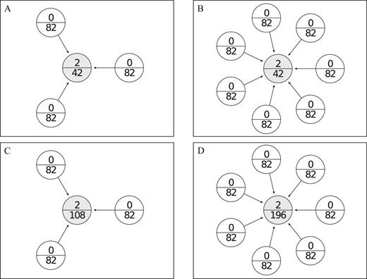
Nash star networks. Graphs show equilibrium Nash star networks of the GG model with n = 4 and n = 8 players. Nodes represent the players. Arrows represent the links and point away from the player who formed the link. The top number in each node indicates the public good investment by the player and the lower number indicates the payoff. Panels A and B illustrate the Nash stars for our treatments without status rents and panels C and D illustrate the treatments with medium status rents.
Important for our purpose is that GG’s main result is unaffected by the introduction of status rents. Panels C and D illustrate the strategic consequences of the introduction of status rents. In these examples, a player receives a payoff of 22 for each incoming link. Notice that compared to the situation without status rents, the core position has become much more attractive because of the higher earnings. The Nash equilibrium of the stage game, however, is not affected because the status rents result from other players’ linking decisions only.
In this public good environment, efficiency requires higher levels of production than the individually optimal two units. Just like in traditional public goods games, efficient cooperation is not supported in the equilibria of GG’s one-shot game. In contrast, a plethora of equilibria outcomes can be supported in the finitely repeated game that we are interested in. One such outcome involves the efficient provision of the public good almost until the final round. To shed light on which of the many repeated game equilibria is to be expected, we introduce the concept of challenge-freeness. An equilibrium is challenge-free if no player has an incentive to challenge the position of the player who is best off and if this player cannot improve her position without being challenged. The concept predicts whether a repeated game equilibrium will be played, and if so, which one. Challenge-freeness is closely related to the concept of envy-free equilibrium, which has been used to successfully predict the equilibrium that materializes in position auctions (Edelman et al. 2007; Varian 2007).
To apply challenge-freeness to our model, notice that in situations without status rents, the periphery position is more attractive than the core position, as illustrated in the top panels of Figure 1 (players in the periphery of the star earn more than the player in the core). In these circumstances, players prefer others to do the painful job of providing the public good. Even if a star is formed, the person in the core will prefer to challenge the position of any player in the periphery. Without status rents, there is no challenge-free equilibrium, and we predict that the situation is inherently unstable and will result in inefficiency.
With status rents, the core position can become more attractive than a periphery position. Figure 2 provides an example for the eight-player case. Moving across the panels from A to D, we illustrate cases where the public good investment by the core increases from two to five units. This increase is costly for the core but increases the earnings of the periphery players. Note that for the step from four to five units, the aggregate gain for the periphery (24) is insufficient to compensate for the 52 lost by the core. The efficient production level in this example is thus four units. We call networks as in panels B, C, D “superstars”, which are star networks in which the core player invests in more units of the public good than is expected in the stage game equilibrium.
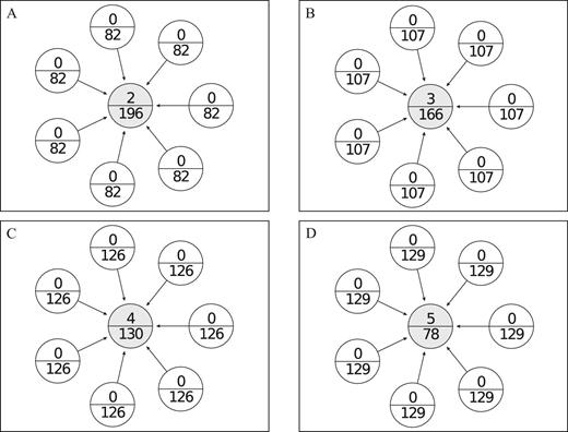
Increased investment in star networks. Graphs show star networks with n = 8 players. The top number in each node indicates the public good investment by the player and the lower number indicates the payoff. The example corresponds to the payoffs for our treatment with 8 players and medium status rents. Panel A is the Nash star network: the core earns more than the periphery. Panels B, C, and D illustrate (super)stars with increasing investment by the core. Payoffs between the core and periphery players are roughly equalized when the core invests in 4 units (panel C).
When the core earns more than the periphery, players may compete to be in the core. The person who is willing to invest most in the public good will subsequently attract all links and become the core player in a star network. This competition for status forces the core player to invest up to the level where payoffs across network positions are roughly equalized, that is, to the point where periphery players no longer have an incentive to challenge the core player by investing more. In the example of Figure 2, the core player has to invest in four units to avoid being challenged.
In the laboratory, we consider two network characteristics that may affect public good provision and the structure and stability of the network. The first is the extent of status rents that a player derives from incoming links; these are absent, of medium value or of high value. The second characteristic is group size, which is either small (four players) or large (eight players). In a full 3 × 2 design, we systematically vary status rents and group size in such a way that leaves the (stage-game) equilibrium predictions of the GG model unaffected. In contrast, challenge-freeness predicts that behavior will vary systematically across our two treatment dimensions. Only with sufficiently large status rents do we predict convergence to a stable core-periphery network. The particular equilibrium selected depends on the two characteristics. Essentially, provision of the public good benefits from an increase in status rents per link as well as from an increase in group size.
Finally, we add two control treatments to the design, in which the network structure is exogenously imposed and based on actual networks formed in the endogenous counterparts. This allows us to isolate the competition-for-status explanation from other possible explanations for contributions by the core (e.g., specific kinds of other-regarding preferences).
In our experiments, we implement the game in a straightforward manner. Subjects participate in only one of the eight (3 × 2 + 2) treatments. They are informed that they remain in the same group for 75 periods and they are informed of the relevant parameters. They know that they have access to their own public good investments and to the investments of the players to whom they have created links. In each period, subjects simultaneously make their links and investment decisions (except in the control treatments, where they only make investment decisions).
Our experimental results for the treatments with endogenous network formation provide clear evidence that participants compete for status rents. In line with the theoretical predictions, stable star networks form only when status rents exist and the extent of such rents and group size both boost the provision of the public good. Without status rents, star networks are observed in only 10% of the cases even in the final 25 periods. This means that in almost all of these cases, networks are formed with too few or too many links, and too many or too few players invest in the public good. As a result, subjects access on average less of the public good than the stage-game Nash amount. Moreover, outcomes are highly inefficient and average experimental earnings are even below what could be expected if there were no scope for networks to form. At the other extreme (with high status rents), in the final 25 periods subjects in the core of a star contribute close to the efficient amount (on average 97% of the efficient amount) when groups are small and they vastly overcontribute when groups are large (on average 173% of the efficient amount). In these cases a star network is formed in 53% and 86% of the cases, respectively. The observed large and positive effect of group size on contributions is in sharp contrast to previous experiments on supergame effects. Finally, not only in the treatments with high status rents, but also in the treatment with medium status rents and large groups, do we observe that groups mostly converge to superstars.
Groups tend to converge to the repeated game equilibria selected by the challenge-freeness refinement. Further support comes from the process by which this occurs. In the first half of the treatments with high status rents, in most groups multiple subjects compete by investing heavily in the public good, challenging each other for an attractive position. They converge to a (challenge-free) superstar in the second half of the experiment. Finally, our results confirm a central prediction of the GG model, which is that the maximum number of players who invest and form the core is independent of group size.
The results for the endogenous network formation treatments are consistent with the hypothesis that players compete for status. There are, however, other possible explanations for our results. Bloch and Jackson (2007) argue that an exchange of transfers can lead to efficiency gains in repeated network games. In the environment of our experiment this would imply that the periphery offers to the core the benefits of an incoming link in exchange for the core providing to the periphery the benefits of a higher investment in the public good. Relatedly, core players may feel that it is their duty to reciprocate by investing more in the public good if they receive high rents from incoming links. Or, altruism or inequity aversion may motivate them to share some of the windfall gains that high status rents bring. Notice that none of these alternative mechanisms requires that the network is endogenously formed. In contrast, challenge-freeness predicts no supergame effects when players participate in an exogenously determined network. In an exogenously formed network, players cannot compete for a favorable position. The player in the core does not face the danger of being challenged and is therefore not encouraged to invest in more than the stage-game Nash amount. Our two control treatments with exogenous networks therefore allow us to isolate the predictions derived from challenge-freeness from the alternatives discussed previously.
The results for these controls provide support for our conjecture that supergame effects are primarily driven by the competition for status. We observe many more superstars when networks are formed endogenously than when they are exogenously imposed. In comparison, the positive role of social preferences is negligible. With exogenous networks, only a handful of prosocially motivated core players contribute more than would be expected on the basis of selfishness. We conclude that the formation of efficient star networks—and other superstars—requires status rents; these trigger competition between the players, which has a substantial impact on the provision level of the public good, and on the shape and stability of the network.
The remainder of this paper is structured as follows. We continue with a brief discussion of previous studies in Section 2. We present the theoretical framework in Section 3. Section 4 describes the experimental design and procedures and in Section 5 we provide equilibrium and efficiency predictions for the game with the parameters of the experiment. The results of the experiment are described in Section 6 and Section 7 concludes.2
2. Literature Review
There is a relatively large theoretical literature on network formation and the provision of public goods in networks, either with endogenously formed networks or exogenously given networks.3 Most relevant for our study is GG (Galeotti and Goyal 2010), who extend the network public goods game of Bramoullé and Kranton (2007) by adding endogenous network formation using the protocol designed by Bala and Goyal (2000). As mentioned previously, we employ the GG framework in our experiment.
Closest to the current study are two other papers that use the GG-framework in laboratory experiments. Both papers focus on other treatment variables than we do. The first is Rong and Houser (2015), who use the best-shot version of the GG-model, that is, players face a binary choice whether or not to invest. In their setup, the public good is provided if and only if at least one of the ex ante homogeneous players invests. Between treatments, they investigate the effect of sequential decision-making and they vary the strategy set of the players. With sequential decision-making, each subject is informed of the all choices of her predecessors. Surprisingly, sequential decision-making does not facilitate the emergence of efficient stable star networks. They vary the strategy set by, first, limiting subjects to either investing or making a link to one other subject; and second, allowing at most one player at a time to contribute to the public good. This restricted strategy set yields more equilibrium (star) networks.
The second related paper is by Goyal et al. (2017), who study the effects of varying the linking costs and of introducing individual heterogeneity. Some of their findings are in agreement with the predictions of the GG-model. For example, they find that increased linking costs lead to fewer links and higher investments by subjects in the core. In the treatments where a single individual has lower linking costs than the others, this subject is more likely to end up in the core, as predicted. At the same time, aggregate investments are higher than predicted and, in contrast to the GG-model, increase with linking costs.4
The results of Goyal et al. (2017) and those of the baseline treatment in Rong and Houser (2015) line up well with the results in our treatments without status rents. In all cases, (equilibrium) core-periphery networks are rarely observed and efficiency is low due to the ineffective network structures. Our paper provides two novel insights compared to these papers. First, we show how stable star networks among ex ante symmetric players can result without restricting subjects’ strategy sets. Second, we identify conditions under which supergame effects are expected.
In our setup, players decide both on their network connections and their investments in a (local) public good where investments are strategic substitutes. These two elements have also been studied in isolation. In experiments purely concerned with network formation (i.e., players only decide on their links) a typical result is that groups rarely converge to equilibrium (star) networks when equilibrium payoffs between different positions are asymmetric (Falk and Kosfeld 2012). Introducing heterogeneity in values can reduce payoff asymmetries; as a result star networks form more often (Goeree et al. 2009). Other experimental studies consider public good games with strategic substitutes, but on fixed networks (Rosenkranz and Weitzel 2012; Charness et al. 2014).5
To the best of our knowledge, we are the first to study endogenous network formation in combination with public goods investment and status rents. Our introduction and analysis of status rents also sheds light on results observed in previous field and laboratory studies. In a natural field experiment, Zhang and Zhu (2011) investigate contributions to Chinese Wikipedia. They interpret the repeated blockings of Chinese Wikipedia in Mainland China as an exogenous variation in group size and observe that contributions increase when groups are larger. Restivo and van de Rijt (2012) provide an example of how status rents may be operationalized in the field. They show that informal rewards (“barnstars”) encourage contributors on Wikipedia to increase their contributions. Algan et al. (2013) run experiments using a large sample of active Wikipedia contributors. Combining experimental and observational data from Wikipedia, they find that high contributions are strongly correlated with social image concerns, but not with altruism. In laboratory experiments, providing rankings based on prosocial behavior can positively affect giving in dictator games (Duffy and Kornienko 2010). Finally, the positive effect that intergroup competition has on cooperation (e.g., Bornstein et al. 1990; Schram and Sonnemans 1996; Nalbantian and Schotter 1997; Reuben and Tyran 2010) may also be attributable to intragroup status.
Aside from status rents, one could interpret the benefits from an incoming link as a transfer between players. Transfers (or side payments) can be an effective way to sustain otherwise unstable networks (Jackson and Wolinsky 1996; Bloch and Jackson 2007). However, our focus is on the competition for links that arise when there are status rents. This turns out to be important. Our two control treatments show that supergame effects are not observed without such competition.
3. Theory
3.1. Stage Game and Static Analysis
We study the one-way flow variant of the static game in GG and extend the model to allow players to enjoy status rents for each incoming link. Wherever possible, we follow the notation in GG.
Denote the set of players by N = {1, 2, …, n}. Every player i ∈ N simultaneously decides on her (public good) investment level xi and the links gi that she forms. Investments are non-negative integers, that is, players select their investments from the set X = {0, 1, 2, …, xmax}. The vector gi = (|${g}$|i,1, |${g}$|i,2, …, |${g}$|i,n) specifies the links that i forms, where |${g}$|i,j = 1 if i forms a link to j and |${g}$|i,j = 0 if not. Hence, a strategy for player i consists of the combination of her public good investment and links and we denote this by si = (gi, xi), and i’s strategy space is denoted by Si. The linking decisions of all players jointly define the (directed) network architecture g = (g1, g2, …, gn) and x = (x1, x2, …, xn) denotes the vector of investments. A strategy profile is then denoted by s = (x, g). The set of all possible strategy profiles is denoted by S.
Forming a link to another player j allows i to access j’s investment. Let Ni (g) = {j ∈ N: |${g}$|i,j = 1} denote the set of players that i links to and ηi(g) = |Ni(g)| is the out degree of i and ωi(g) = | j ∈ N: |${g}$|j,i = 1| is the in degree of i. The total investment that i accesses is then given by |${y_i} = {x_i}{\rm{\ }} + \mathop \sum \nolimits_{j \in {N_i}( {{\boldsymbol g}} )} {x_j}$|. The benefits f(yi) of accessing units are increasing and concave in yi, and f (0) = 0. Note that the investments of i and of the players she has linked to are perfect substitutes: i values her own investment the same as any investments by any j ∈ Ni(g).
In a core-periphery network, players are in either the core or the periphery of the network, and players in either group form links exclusively to the (other) core player(s). This is, if we denote the set of players who are in the core by |${\what{N}_C}( {{\boldsymbol g}} )$| and the set of those in the periphery by |${\what{N}_P}( {{\boldsymbol g}} )$|, then |${N_i}({{\boldsymbol g}} ) = {\what{N}_C} ( {{\boldsymbol g}} )\backslash \{ i \}\ \forall \ i \in {\what{N}_C}( {{\boldsymbol g}} )$| and |${N_j}( {{\boldsymbol g}} ) = {\what{N}_C} ( {{\boldsymbol g}} )\ \forall \ j \in {\what{N}_P}( {{\boldsymbol g}} )$|. The main result in GG is that in any strict Nash equilibrium, a core-periphery network is formed, where the players in the core invest in the public good and players in the periphery do not invest. The proof of this and subsequent results is relegated to Appendix A.6 In equilibrium, the players in the core jointly invest in |$\hat{y}$| units, where |$\hat{y}$| is defined as the optimal public good investment if players were to act in isolation, that is, |$\hat{y} = \arg \mathop {\max }\nolimits_{{x_{{i}}} \in X} ( {f( {{x_i}} ) - c{x_i}} )$|. The maximal number of players that can be sustained in the core (and invest) is independent of group size and status rents. A special case is the Nash star. In this outcome, a single player forms the core and invests in |$\hat{y}$| units. Whenever we refer to “stars”, we always mean periphery-sponsored stars.
If |$c\hat{y} > k$|, the Nash star is always a strict Nash equilibrium.7 The intuition is the following. The marginal benefits of the public good exceed the costs of investing in up to |$\hat{y}$| units of the good. This implies that every player wants to access at least |$\hat{y}$| units of the good. Suppose there exists some player i that invests in |$\hat{y}$| units. When forming a link is strictly less costly than investing in |$\hat{y}$| units, that is, |$c\hat{y} > k$|, the best response of any other player than i would be to link to i and not invest, hence a star forms where the core invests and all others free-ride and link to the core.8 Finally, for i, given that no other player is investing, it is optimal to invest in |$\hat{y}$| units. There are n such equilibria: one for each player being in the core.
As the strategies of all other players are fixed, it must be that ωi(g) = ωi(g′) and the final term on the left hand side of (1) cancels. Then, i’s decision is independent of the status rents b and the set of Nash equilibria must be independent of b.
Based on this definition, the efficient outcome is a star in which the core player invests in (weakly) more units than in the Nash star, whereas the periphery players do not invest. This is the case because all players—either in the periphery or the core—benefit from additional investments by the core. The efficient investment by the core is denoted by |$\tilde{y} \ge \hat{y}$| (see Appendix A). Note that any investment by the core above |$\tilde{y}$| units will lead to welfare losses. In the Introduction, we informally defined superstars. More formally, we call an outcome a superstar if it is a star where the core invests in strictly more units than in the Nash star. Note that efficient outcomes are superstars if |$\tilde{y} > \hat{y}$|.
3.2. Subgame Perfect Equilibria
In this section, we discuss some equilibria of the finitely repeated game that we study in the experiment. It is well known that that the repeated game hosts a plethora of subgame perfect equilibria if the stage game has multiple Nash equilibria (Benoit and Krishna 1985). In particular, more cooperative outcomes than the repeated play of a stage game equilibrium can be supported, because a deviating player can credibly be punished if the others coordinate on her worst possible stage-game equilibrium. In fact, Benoit and Krishna (1985) show that even more severe punishments than the worst stage-game outcome are possible for longer horizons.
The Benoit and Krishna (1985) result applies directly to our finitely repeated game. The stage-game hosts (at least) n equilibria, one for each player being in the core of a Nash star. In the Nash star, there are two payoff levels: one for the player in the core and one for those in the periphery. Repeated game equilibria can be constructed that are either better or worse in terms of joint payoffs than repeated play of a stage game equilibrium. Here, we first focus on a class of equilibria where the core position rotates. A rotating core is most conducive to support cooperative outcomes in equilibrium, but requires tremendous coordination. Then we present the class of equilibria in which the network remains fixed. The latter class is particularly relevant for the concept of challenge-freeness that will be introduced in the next section. Online Appendix D provides more details.9
To present the repeated game analysis, we introduce some additional notation. Denote the T-fold repetition of the stage-game by G(T) and denote the repeated game strategy of i by σi. In the repeated game, a strategy σi specifies an action for any history of play. A strategy profile σ is the n-tuple of repeated game strategies. Such a strategy profile induces an outcome path (s1, s2, …, sT), where st is the stage-game outcome of period t. Denote the history in period K by h(K) = (s1, s2, …, sK).
Let σ||h(K) denote the strategy profile for the subgame G(T − K) that is induced by σ after observing h(K). Then, σ constitutes a subgame perfect equilibrium of G(T) if (i) it is a Nash equilibrium of G(T) and (ii) if σ||h(K) is also a Nash equilibrium of G(T − K) after every possible h(K) at any K < T. One subgame perfect equilibrium of G(T) is a stationary repetition of a stage-game Nash equilibrium (a Nash star). Subgame perfect equilibria with superstars also exist, however.
One way to support superstars in a subgame perfect equilibrium is by rotating the core position. Rotating means that a star network is formed in every period, but players take turns in filling the core position, that is, there exists a sequence |$\{ {1,2, \ldots ,n,1,2 \ldots} \}_{t = 1}^{t = T}$| that determines who will be in the core. This is formally established in Proposition 1.
If G(T) is sufficiently long, efficient superstars with a rotating core position can be supported as part of a subgame perfect equilibrium until period T − Q, where 1 ≤ Q < T.
In Online Appendix D we provide a proof and specify how long G(T) should be for Proposition 1 to hold. The intuition underlying Proposition 1 is that G(T) can be split in two phases. In the first T − Q periods, the efficient superstar is formed with players taking turns being in the core. In the final Q periods, a Nash star is formed where players again take turns filling the core position. Key is that in these final Q periods, players earn strictly more than in their worst stage-game outcome, as at least for some periods they are in either the core or the periphery (whichever is better).
Rotating the core of the Nash star can also be used to construct subgame perfect equilibria that have lower joint payoffs than repeated play of the Nash star. For instance, consider a strategy profile that induces an empty network without any links and investments in the first T − Q periods, and a Nash star with a rotating core in the final Q periods. This means that W = 0 in the first T − Q periods, and joint payoffs across all periods must be lower than under repeated play of the Nash star. In Online Appendix D we show that this type of equilibria exists both with and without status rents.
Such rotation requires tremendous coordination, however, and is unlikely to be observed in laboratory play (e.g. Goeree et al. 2009; Falk and Kosfeld 2012). If we consider only subgame perfect equilibria without rotation—that is, each player forms the same links in all periods on the equilibrium path—we obtain the following result.
If no player ever changes their linking decisions on the equilibrium path, then status rents are necessary for the formation of superstars in a subgame perfect equilibrium.
A proof is provided in Online Appendix D. Here we provide the intuition for a repeated game with only two periods. In the absence of status rents, the worst stage game outcome is the core position in the Nash star. Proposition 2 requires that the same player i is in the core of the star in all periods of G(T). Hence, in any subgame perfect equilibrium, the final period of G(T) must be the Nash star with i in the core. As the payoff in the final period T = 2 equals the worst stage game payoff of i, she will not be willing to invest above the Nash amount in the first period. This is different when there are status rents. If status rents are sufficiently large, the periphery earns less than the core in the Nash star. Then, the threat of being in the periphery rather than the core in the final period is sufficient to make i invest above the stage game Nash level in the first period. In Online Appendix D, we extend this argument to G(T) of any finite length.
Although status rents affect the set of repeated-game equilibria, subgame perfection in itself provides little guidance on which equilibrium, if any, to expect. As argued previously, we hypothesize that players will compete for attractive network positions. We capture this hypothesis with the simple concept of challenge-freeness. Challenge-freeness is a notion of stability that we use to derive predictions for the experimental treatments. If an outcome is not challenge-free, it is easy to see how an external challenge or an internal adjustment becomes attractive that will change the outcome.
3.3. Challenge-Freeness
Since Tinbergen (1946), the concept of envy-freeness has become a cornerstone in the economic theory of distributive justice. According to this criterion, no agent should prefer any of her neighbor's allocations to her own (see Arnsperger 1994 for a survey of the early literature). In more recent contributions, envy freeness has been employed as a criterion for equilibrium selection in position auctions (independently by Edelman et al. 2007; Varian 2007).10
In a similar vein, our concept of challenge-freeness is motivated by the idea that players compete for attractive positions. Applied to the GG-model, our intuition is that an outcome is stable if players have no desire to challenge the position of the player with the best payoff in the network. In this line of reasoning, large payoff differences with the top earner lead to instability, because players are tempted to “challenge” this player's position.
Status rents do not affect the set of stage-game equilibria, but they do affect the payoffs of players in the core. In any strict Nash equilibrium of our stage game, the core players earn less than the periphery players in the absence of status rents. Introducing status rents increases the payoffs of core players, without affecting those of the players in the periphery. The size of the effect of status rents on core payoffs depends on group size. Status rents and group size jointly determine the relative payoffs between players in the periphery and the core. The main idea is that if the payoffs of the core are (sufficiently) larger than the payoffs of periphery players, those in the periphery will want to challenge the position of the core player. In this game, they can do so by investing in one more unit than the core. The only way in which the core player can avoid being challenged is by choosing an investment level that makes investing in the extra unit unattractive (compared to what other players receive when they stay in the periphery). Only if the core invests an amount that is sufficient to (almost) equalize payoffs, a network can be challenge-free.
Let b−i,−1(s1, si, s−1,−i) be the collection of bj that minimizes |${\Pi _i}( {{s_1},s_i^{\prime},{{\boldsymbol{b}}_{ - i,\ - 1}}} )$|. This means that if the best response bj of player j is not unique, i is pessimistic and assigns the worst possible (stage game) payoff to the outcome. For the game under consideration, this pessimism means that player i acts as if she can only attract the links of the core player if she invests strictly more than the core player does. Hence, given s1, player i believes that changing to strategy |${s_{i}^{\prime}}$| will lead to the stage-game outcome induced by strategy profile s′ = (s1, |${s_{i}^{\prime}}$|, b−i,−1). If for all |${s_{i}^{\prime}}$| this will not lead to a higher payoff than in the current stage-game outcome that follows from s, i will not challenge player 1. The second ingredient for challenge-freeness is that player 1 cannot improve her payoff without being challenged. We now define a challenge-free outcome in the following way.
A stage game outcome, induced by a stage-game strategy profiles*, is challenge-free if and only if
(i) no player wants to challenge player 1, who has the highest payoff, which means that for each player i (i > 1): Πi(s*) ≥ |${\Pi _i}( {s_1^{\rm{*}},{{s}_{i}^{\prime}},{{\boldsymbol{b}}_{-i,-1}}{\rm{\ }}} ),{\rm{\ }}\forall {s_{i}^{\prime}}$| ∈ |${S_i}$| , and
(ii) player 1 cannot improve her payoff without being challenged. That is, for all |${s_{1}^{\prime}}$| ∈ S1 such that |${\Pi _1}( {s_1^{\rm{*}},\ {{\boldsymbol s}}_{ - 1}^{\rm{*}}} ) < {\Pi _1}( {{{s}_{1}^{\prime}},\ {{\boldsymbol s}}_{ - 1}^{\rm{*}}} )$|, there exists a player i and a strategy |${s_{i}^{\prime}}$| ∈ Si such that |${\Pi _i}( {{{s}_{1}^{\prime}},\ {{\boldsymbol s}}_{-1}^{\rm{*}}} )$| < Πi (|${s_{1}^{\prime}}$|, |${s_{i}^{\prime}}$|, b−i,−1) and |${\Pi _1}( {s_1^{\rm{*}},\ {\boldsymbol{s}}_{-1}^{\rm{*}}} ) > {\Pi _1}$| (|${s_{1}^{\prime}}$|, |${s_{i}^{\prime}}$|, b−i,−1).11
Next, we discuss the conditions under which Nash stars and superstars are challenge-free. For the analysis, we make a simplifying assumption. The assumption is fulfilled in the parameterization in our experiment.
Linking costs are sufficiently large: (i) k > f(x + x′) − f(x) if|$x \ge \hat{y}$|and x ≥ x′; (ii) |$k > c( {\hat{y} - 1} )$|.
The first part of Assumption 1 ensures that no player will link to multiple players if there exists some player that invested in at least |$\hat{y}$|. The second part of the assumption prevents that networks with multiple hubs are formed in a stage-game equilibrium, as the inequality implies that if a player i invests in at most |$( {\hat{y} - 1} )$|, none of the other players will link to i.
Consider a star where the core invests in xc units and all periphery players do not invest. Call this network the xc-star. Note that there are only two payoff levels in this case: core and periphery. The stage-game payoffs for the core player are given by πc = f(xc) − cxc + (n − 1)b and the stage-game payoffs for the each periphery player by πp = f(xc) − k.
If (2) holds, the core player will not be challenged. Note that the RHS of (2) is strictly increasing in xc for |${x_c} \ge \hat{y}$|, because by construction c > f(xc + 1) − f(xc) for investments larger than or equal to the Nash quantity |$\hat{y}.$| Denote the lowest value of xc for which (2) holds by y*. In the y*-star the core invests so much that the payoffs are almost equalized and that the periphery lacks an incentive to challenge the core.
Figure 3 illustrates challenging in four-player star networks. In panel A, the core invests in three units and earns more than the periphery players do. Panel B shows that if a periphery player (the black node) challenges the core by investing in four units, she assumes that the other two periphery players will move their links to her, leading to a higher payoff than in the star network of panel A. Hence, the star network of panel A is not challenge-free. The star network of panel C is challenge-free. In this case, the core player invests in four units and earns more than the periphery players do. Challenging the core by investing in five units leads to a lower payoff for a challenging periphery player, and therefore none of the periphery players will challenge the core player. For the star in panel C of Figure 3 to be challenge-free, part (ii) of Definition 1 should also be satisfied. For the parameters of the example of Figure 3 this is the case: the core player could improve her payoff by lowering her investment (see panel A), but this would lead to a challenge by the periphery players (see panel B).
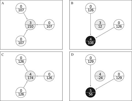
Challenging in star networks. The star network in panel A is not challenge-free. Panel B shows that a periphery player will challenge the core as this leads to a higher payoff than the periphery payoff in panel A. The star network in panel C is challenge-free. In this case, challenging will lead to lower payoffs for the challenger (panel D) and the core player cannot improve her payoff without being challenged. In each panel, the top number in each node indicates the public good investment by the player and the lower number indicates the payoff. The example corresponds to the payoffs for our treatment with 4 players and high status rents.
When there are no status rents, or when status rents are low, the core earns less than the periphery in the Nash star. This happens when |$( {n - 1} )b < c\hat{y} - k$|. In this case, a Nash star or superstar can only be challenge-free if the core does not want to challenge the periphery. We find that this is never the case. Consider the Nash star, that is, |${x_c} = \hat{y}$|. Core player i > 1 can challenge player 1 in the periphery by lowering her investment, for instance to xi = 0, and linking to one of the other periphery players j > 1. If she does so, player 1 whom she challenges will be committed to not investing (and linking to i), but any other periphery player j > 1 is expected to best respond by investing in |$\hat{y}$| units and forming no links. In this case, i will earn |$\Pi( {{{\boldsymbol s^{\prime}}}} ) = \ f( {\hat{y}} ) - k + b$|, which is larger than the payoff she earned as the core player. This means that the Nash star cannot be challenge-free if the core earns less than the periphery. As the core in a superstar earns less than the core in the Nash star, the same argument applies here. Hence, if status rents are low or absent, Nash stars and superstars are not challenge-free. Proposition 3 summarizes what is needed for the existence of a challenge-free outcome, and it characterizes the challenge-free outcome if it exists.
The existence of a challenge-free outcome depends on the extent of the status rents.
(i) If status rents are sufficiently high, that is, when the core earns more than a player in the periphery in the Nash star, the only challenge-free outcome is a star where the core player invests in|${x_c} = \max ( {\hat{y},{y^{\rm{*}}}} )$|, and the periphery players do not invest.
(ii) If status rents are low, that is, when the core earns less than a player in the periphery in the Nash star, there is no challenge-free outcome.
In Appendix B we provide a proof.12
A challenge-free equilibrium implements a challenge-free outcome in every stage, except in the final stage(s) of the game. The key-predictions that we will test in the experiment are: (i) Without sufficient status rents, there is no challenge-free outcome and as a result we predict that the experimental results are unstable. (ii) With sufficient status rents, a challenge-free outcome will emerge. Whether the network is predicted to be characterized by underprovision, efficient provision or overprovision of the public good will depend on the combination of status rents and group size. The concept of challenge-freeness will also be applied to our treatments with exogenous networks. In this case, a periphery player cannot successfully challenge the core by investing more than the core. Hence, any Nash star is challenge-free, even if the core earns substantially more than the periphery. In Section 5, we make these predictions precise after having introduced the specific parameters of the experimental design.
The way we have defined challenging is specific enough to make clear predictions, but also general enough to be applicable to other settings. In laboratory settings that employ the GG-framework (Rong and Houser 2015; Goyal et al. 2017), the only challenge-free Nash equilibria are Nash stars in the treatments with “investment limits” by Rong and Houser (2015). These are far more frequently formed than Nash equilibria that are not challenge-free across the two studies. Also in settings with public good provision on fixed networks, challenge-freeness organizes the data well. Rosenkranz and Weitzel (2012) find that across several exogenous networks with two-way flow, the most stable Nash equilibrium is a star where the periphery invests and the core free-rides. This is the only challenge-free equilibrium across all (exogenous) networks. Falk and Kosfeld (2012) compare pure network formation with one-way flow and two-way flow and find that Nash networks form much more frequently under one-way flow. This is exactly what challenge-freeness predicts. Finally, the findings by Goeree et al. (2009) are not completely in line with challenge-freeness. The most frequently observed network in their treatments with heterogeneous players is a periphery-sponsored star with a high-value player in the core. This network is challenge-free. In their baseline treatment with homogeneous players, however, periphery-sponsored stars are also challenge-free, but these are rarely observed in the experiment.
4. Experimental Design and Procedures
In the experiment, subjects play the stage-game described in Section 3 repeatedly for 75 periods. Across treatments, we systematically vary two parameters: group size n and the level of status rents b. Table 1 summarizes this design: we have groups of either 4 or 8 subjects, who play the experimental game either with no (b = 0), medium (b = 22), or high (b = 66) status rents. In addition, we ran two treatments with high status rents where the links are exogenously imposed.
Overview of treatments.
| Endogenous networks | Exogenous networks | ||||
|---|---|---|---|---|---|
| Treatment variable | Small group size n = 4 | Large group size n = 8 | Small group size n = 4 | Large group size n = 8 | |
| No status rents | b = 0 | n4b0 | n8b0 | ||
| 8 groups | 6 groups | ||||
| 32 subjects | 48 subjects | ||||
| Medium status rents | b = 22 | n4b0 | n8b22 | ||
| 8 groups | 6 groups | ||||
| 32 subjects | 48 subjects | ||||
| Large status rents | b = 66 | n4b66 | n8b66 | n4b66EXO | n8b66EXO |
| 8 groups | 6 groups | 8 groups | 6 groups | ||
| 32 subjects | 48 subjects | 32 subjects | 48 subjects | ||
Notes: The first line in a cell list depicts the treatment acronym (the first part refers to group size and the second to the status rents); the lower lines give the number of groups and subjects in each treatment.
In the treatments with endogenous network formation we implement a partners design: that is, subjects are randomly assigned to a group and play the experimental game with fixed partners.13 These partners are identified by letters ranging from A to D or A to H, depending on the group size and the letters refer to the same subject throughout the experiment. The number of periods is announced in the experimental instructions (see Online Appendix E).
In every period, all subjects simultaneously decide on whom to link to and how much to invest.14 On their decision screen, subjects can review all previous decisions in a history box. Once everyone in the session has made a decision, subjects are informed of the resulting outcome and their own payoffs. Examples of key screenshots are provided in Online Appendix F.
In the treatments with exogenous linking, everything is the same as in the treatments with endogenous linking except that we impose the linking decisions previously observed in the endogenous linking treatments. Hence, in the treatments with exogenous networks, subjects face exactly the same link structures as subjects in the corresponding endogenous network treatments. Subjects are informed of the links they will form in the current period and only decide on their investment in the public good. In the instructions, subjects are informed that they could in no way affect the links by their decisions. Note that subjects do pay for outgoing links and receive rents for incoming links. As with endogenous linking, subjects have access to the history box.
In all treatments, earnings are denoted in “points”. In addition to a starting capital of 2000 points, subjects may earn points in every period. Total point earnings are exchanged at the end of the experiment at a rate of €0.10 for every 30 points. Table 2 gives the benefits function f(yi) (in points), as well as the costs of linking, k, the costs of investment c and the status rents b. As specified in Section 3, the function f(yi) is increasing and concave in yi, and k > b.
Benefit and cost parameters in the experiment.
| Panel a: Benefits from accessing the public good | |||||||||
| Units accessed yi | 0 | 1 | 2 | 3 | 4 | 5 | 6 | 7 | 7+ℓ |
| Benefits f(yi) | 0 | 92 | 152 | 177 | 196 | 199 | 202 | 203 | 203+ℓ |
| Marginal benefits | 92 | 60 | 25 | 19 | 3 | 3 | 1 | 1 | |
| Panel b: Cost and benefits of investing and linking | |||||||||
| Status rents | |||||||||
| None | Medium | High | |||||||
| Cost per unit investment c | 55 | 55 | 55 | ||||||
| Cost per link made k | 70 | 70 | 70 | ||||||
| Benefit per link received b | 0 | 22 | 66 | ||||||
Sessions were run between May and July 2014 in the CREED laboratory of the University of Amsterdam and lasted about two hours. For each treatment with n = 4, we had a total of 8 groups whereas we had 6 groups for each treatment with n = 8. In total, 320 subjects participated in the experiment, each in only one session. We conducted 15 sessions where, depending on show-up, the number of subjects per session varied between 12 and 32, but in most sessions 24 subjects participated. We randomized treatments within a session: in each session with endogenous network formation at least two different treatments were conducted. Each subject participated in one treatment only. Subjects were recruited from the local CREED database, which consists mostly of undergraduate students from various fields. Of the subjects in our experiments, 49% are female and 61% were studying at the Amsterdam School of Economics or the Amsterdam Business School. Cash earnings were between €5.70 and €125.50, with a mean of €30.63.
The experiment was computerized using PHP/MySQL and was conducted in English. Upon entering the laboratory, subjects were randomly allocated to a separate cubicle. Communication was prohibited throughout the session. Before starting the network experiment, we elicited risk preferences using a procedure similar to Gneezy and Potters (1997). In this procedure, each subject decided how much to invest of a capital of 600 points. The amount invested was lost or multiplied by 2.5 with equal probability. The result of the investment was then added to the amount not invested. Subjects were only informed of the outcome of this part at the very end of the experiment.
After this, subjects read the instructions of the network game at their own pace, on-screen. While reading the instructions, a printed summary was handed out. To ensure that all subjects understood the instructions, they were required to answer several test questions (cf. Online Appendix E). The experiment did not continue before everyone had answered all questions correctly.
We ended each session with a short questionnaire after which we privately informed subjects of the outcome of the risk elicitation task and their aggregate earnings in the experiment. Subjects were privately paid in cash for all periods of the network game and the risk-elicitation task.
5. Predictions for the Experiment
In all experimental treatments with endogenous linking, the Nash equilibria of the stage game are the same. As argued in Section 3.1, the set of stage-game Nash equilibria is independent of our treatment variables; status rents and group size (how the set of subgame perfect equilibria in the repeated game is affected is discussed in Online Appendix D). Figure 1 illustrates these equilibria for the treatments with no status rents (panels A and B) and medium status rents (panels C and D). We observe a Nash star, where the core player invests in |$\hat{y} = \ 2$| units and the other players form links to the core and do not invest. Furthermore, the efficient outcome is also the same across treatments: in all cases it is a superstar where the core invests in |$\tilde{y} = 4$| units (Figure 2, panel C). As noted before, status rents and group size do not affect the set of stage-game equilibria, but they do affect the payoffs of players in the core. The lower numbers inside each circle represent the payoffs.15 These payoff differences determine whether stars are challenge-free, and therefore provide a prediction for the investment by the core player.
Table 3 summarizes the predictions based on challenge-free outcomes (cf. Appendix B). To start, recall that without status rents the core earns less than the periphery and will prefer to lower her investment to zero, expecting that some other player will invest the Nash amount of 2 units. As we show in Appendix B, no network is challenge-free for these treatments. Therefore, we do not expect that stable networks will form in the absence of status rents.
Behavioral predictions.
| Endogenous networks | Exogenous networks | |||||||
|---|---|---|---|---|---|---|---|---|
| n4b0 | n8b0 | n4b22 | n8b22 | n4b66 | n8b66 | n4b0 EXO | n8b0 EXO | |
| y* | 2 | 2 | 2 | 4 | 4 | 8 | 2 | 2 |
| Prediction | Instability | Instability | 2-star | 4-star | 4-star | 8-star | 2-star | 2-star |
| Endogenous networks | Exogenous networks | |||||||
|---|---|---|---|---|---|---|---|---|
| n4b0 | n8b0 | n4b22 | n8b22 | n4b66 | n8b66 | n4b0 EXO | n8b0 EXO | |
| y* | 2 | 2 | 2 | 4 | 4 | 8 | 2 | 2 |
| Prediction | Instability | Instability | 2-star | 4-star | 4-star | 8-star | 2-star | 2-star |
Notes: Columns distinguish between our eight treatments. y* is defined using equation (2). The prediction is the outcome selected by the challenge-free refinement. When stable stars are predicted, they also constitute a subgame perfect equilibrium for the game concerned (cf. Online Appendix D).
This changes when status rents are introduced. In this case, challenge-freeness selects a y*-star. In a dynamic setting, competition for the attractive core position pushes up the investments by the core such that payoffs are almost equalized. In n4b22, we expect stable Nash stars to form. With higher status rents or larger groups, we expect competition for the core position. More specifically, in treatments n8b22 and n4b66 we expect that competition leads to the formation of efficient superstars where the core invests in four units.16 In n8b66, we expect that competition for the core position will be so intense that it encourages severe overinvestment by the core. Here, we expect the emergence of star networks where the core invests in eight units.
6. Results
We have organized the presentation of the experimental results as follows. In Section 6.1, we start with an overview of the outcomes that are observed in our treatments with endogenous network formation. We complement this overview with a discussion of cross-treatment differences in the provision of the public good. Then we provide an overview of the efficiency levels that follow from the networks formed. In Section 6.2, we study the behavioral dynamics in the experiment and compare the outcome to our theoretical predictions. We address the question of which treatments trigger a competition for status, and we present an analysis of the frequency and stability of the outcomes that we observe. Finally, in Section 6.3 we present the results of our exogenous network treatments, which allow us to shed light on the motives underlying our results. Unless stated otherwise, all tests reported are Mann–Whitney tests (henceforth, MW). Throughout, we use two-sided tests using average statistics per group as units of observation.
6.1. Overview: Star Networks and Public Good Provision
Figure 4 plots the relative frequency of stars over time. At the start of the experiment, we hardly observe any stars in any treatment. Starting around period 10, a clear distinction emerges between the two treatments without status rents and those with. With status rents, the frequency of stars steadily increases over time. In the last 25 periods of these treatments, this frequency rises to 76%. In treatment n8b66 stars are even observed in 88% of the last 10 periods. In stark contrast, there is no clear trend in the occurrence of stars in the treatments without status rents. There, such networks remain rare throughout the experiment.
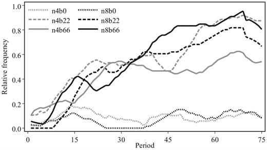
Development of star networks. Lines show the relative frequencies of periphery-sponsored stars by treatment and period. Lines are smoothed by taking the moving average over periods t − 5 to t + 5 for every period t.
Table 4 makes these results more precise and tests whether the observed differences are significant. The table confirms the picture emerging from Figure 4. Stars form substantially and systematically more often in the treatments with status rents than in the treatments without. Within these classes of treatments, differences are much smaller and mostly insignificant.
Frequency of star networks.
| Relative frequency of periphery-sponsored stars | p-values pairwise MW tests | |||||||
|---|---|---|---|---|---|---|---|---|
| Treatment | All periods | Final 25 periods | n4b0 | n8b0 | n4b22 | n8b22 | n4b66 | n8b66 |
| n4b0 | 0.09 | 0.09 | – | |||||
| n8b0 | 0.07 | 0.11 | 0.15 | – | ||||
| n4b22 | 0.58 | 0.86 | 0.00 | 0.00 | – | |||
| n8b22 | 0.50 | 0.73 | 0.04 | 0.02 | 1.00 | – | ||
| n4b66 | 0.43 | 0.53 | 0.09 | 0.09 | 0.32 | 0.61 | – | |
| n8b66 | 0.58 | 0.86 | 0.00 | 0.01 | 0.52 | 0.87 | 0.56 | – |
Notes: The left panel provides the relative frequencies of periphery-sponsored stars in all periods and in the final 25 periods. The right panel provides the results of MW tests for the differences in occurrence between treatments using the observations in all periods. In Appendix C we provide a table with the p-values for differences in the final 25 periods.
Status rents and group size also have profound effects on the provision of the public good. To compare investment choices while holding network composition constant, we focus on the investment of core players in periods where stars were formed. The results are presented in Table 5. This table shows that, conditional on a star being formed, public good provision is inefficiently low (i.e., below four units) in the treatments without rents and the treatment with medium rents and small group size. In treatments n4b66 and n8b22 public good provision is close to the efficient level of four units. In treatment n8b66 the core player vastly overinvests with an average contribution level that is close to double the efficient amount. With status rents, any increase in group size or status rents leads to higher investment by core players. The sizable differences between treatments are all significant, except for the comparisons between n4b0 and n8b0 and between n8b22 and n4b66. By and large, the average and median investment levels accord very well with the predictions based on challenge-freeness.
Investment by core players in star networks.
| Investment in public good | |||||||||
|---|---|---|---|---|---|---|---|---|---|
| (all periods) | p-values pairwise MW tests | ||||||||
| Treatment | Predicted | Mean (se) | Median | n4b0 | n8b0 | n4b22 | n8b22 | n4b66 | n8b66 |
| n4b0 | – | 1.83 (0.11) | 2 | – | |||||
| n8b0 | – | 1.83 (0.09) | 2 | 0.92 | – | ||||
| n4b22 | 2 | 2.22 (0.06) | 2 | 0.01 | 0.02 | – | |||
| n8b22 | 4 | 3.49 (0.33) | 4 | 0.01 | 0.03 | 0.03 | – | ||
| n4b66 | 4 | 3.61 (0.18) | 3.5 | 0.00 | 0.02 | 0.00 | 0.75 | – | |
| n8b66 | 8 | 7.07 (0.46) | 7.5 | 0.00 | 0.02 | 0.00 | 0.00 | 0.00 | – |
Notes: The left panel lists the predicted, mean, and median investment in the public good by core players, conditional on a periphery-sponsored star being formed. The predicted investment is equal to y*, except in the treatments without status rents, where no stable star is predicted. Standard errors of the mean are presented in parentheses, based on mean investments per group. The median is obtained by taking the median within each group first and then the median of these numbers per treatment. The right panel presents p-values for tests whether mean core investments differ between treatments, conditional on a periphery-sponsored star having formed.
Investments in the public good are one of the factors that affect efficiency in this environment. The other is the links made to access the public good. We now consider both factors simultaneously by looking at treatment differences in observed efficiency. Table 6 shows the relative frequency of efficient star networks (where the core invests in 4 units), mean earnings and mean earnings net of status rents per treatment.
Efficiency.
| Efficiency measure | p-values pairwise MW tests for net earnings | ||||||||
|---|---|---|---|---|---|---|---|---|---|
| Treatment | Efficient stars | Mean earnings (se) | Mean net earnings (se) | n4b0 | n8b0 | n4b22 | n8b22 | n4b66 | n8b66 |
| n4b0 | 0.00 | 33.4 (3.0) | 33.4 (3.0) | – | |||||
| n8b0 | 0.00 | 38.9 (1.9) | 38.9 (1.9) | 0.12 | – | ||||
| n4b22 | 0.01 | 75.9 (2.0) | 60.9 (2.0) | 0.00 | 0.00 | – | |||
| n8b22 | 0.32 | 99.9 (4.2) | 81.6 (3.9) | 0.00 | 0.00 | 0.00 | – | ||
| n4b66 | 0.29 | 106.1 (6.4) | 59.7 (6.6) | 0.01 | 0.03 | 0.92 | 0.05 | – | |
| n8b66 | 0.00 | 124.6 (7.4) | 67.9 (6.5) | 0.00 | 0.01 | 0.16 | 0.08 | 0.30 | – |
Notes: The first column gives the relative frequency of efficient outcomes. The efficient outcome is a periphery-sponsored star where the core invests in four units and no periphery player invests. Mean earnings are denoted per subject in points per period. For mean net earnings we subtract the status rents. Standard errors of the means are computed using each group as an individual observation. The panels on the right give p-values for tests whether mean net earnings differ between treatments.
Efficient star networks are almost exclusively observed in n8b22 and n4b66. As noted before (cf. Table 4), stars rarely form at all without status rents. In n4b22, stars are formed but investments by the core are typically lower than the social optimum (cf. Table 5). In n8b66, we also frequently observe stars but here the core vastly overcontributes. As for earnings, as expected, these increase as status rents rise. We correct for this effect of adding money to the system by deducting the status rents from the earnings. This yields a clear difference between the treatments with and without status rents. The treatments without status rents perform particularly badly in terms of (net) earnings. Here subjects do not benefit from interacting with others and actually do worse than if they had completely refrained from making links and simply investing in two units themselves.17 This mirrors previous experimental results reported in the literature on endogenous network formation without status rents (e.g., Falk and Kosfeld 2012). Net earnings are much higher when there are status rents. In pairwise comparisons, either of the treatments without status rents reaches significantly lower net earnings than any of the treatments with status rents (all p < 0.05). Net earnings are the highest in treatment n8b22. This is also the treatment where we observe efficient 4-stars the most frequently. Net earnings are higher in this treatment than in all other treatments (p < 0.10 for all pairwise comparisons).
Next, we turn to the convergence of our data across periods. Figure 5 displays for each treatment the proportion of groups that converge to a stable outcome. If a group converges, it is almost always to a star network.18

Proportion of groups converging and end-point of the dynamics. A group converges to a network if all players repeat decisions at least 5 times. Most groups converge to “x-star” outcomes, periphery-sponsored stars in which the core player invests in x units of the public good. Most groups converge only once: only 4 of the 42 groups converged to two or more different networks. In these cases, we include the last stable network.
Without status rents groups almost never converge to any stable outcome, independent of group size. Moreover, we do not observe any successful rotation of the core position in our experiments. The behavior that is frequently observed is closer to what would be expected in a mixed strategy equilibrium. Subjects switch frequently between not investing and forming a single link, or not linking and investing in 2 units. This is in line with the symmetric mixed strategy equilibrium. In this equilibrium, players randomize between exactly these two possibilities: (i) invest in 2 units and form no links with probability p = 14/19 ≈ 0.737 and (ii) do not invest and form a single link with probability 1 − p = 5/19.19 In the latter case, a player selects randomly any of the others to link to, each with the same probability. Inconsistent with the mixed equilibrium is that our subjects mix with a probability closer to 50% than the equilibrium suggests. In n4b0, subjects invest in 2 units and form links in 42.8% of the cases, and form a single link and do not invest in 42.2% of the cases. In n8b0, this is 31.6% and 54.6%, respectively.
When there are status rents, group size and status rents have a beneficial effect on the provision of the public good. With medium status rents and small groups, groups usually converge to a star network in which the core player consistently invests the stage game Nash amount of two units.20 When group size is doubled in treatment n8b22, all groups converge to a stable network. The most frequently observed end-point of the dynamics is a superstar in which the core player invests the efficient amount of four units. Similarly, with high status rents, investments are higher in large groups than in small groups. In fact, in this case all large groups converge to a star network in which the core player overinvests in the public good. In this treatment, the large majority of groups converge to superstar networks in which the core invests in seven or eight units, which is on average almost double the efficient investment of four units.
These results agree well with the predictions based on challenge-freeness. In accordance with challenge-freeness, stable Nash stars (where the core invests in two units) should only be observed in treatment n4b22 and the occurrence of large overinvestments should be limited to treatment n8b66 (cf. Table 3). Of particular interest is the comparison of treatments n4b66 and n8b22. These treatments allow us to investigate whether the earnings for the player in the core relative to the players in the periphery is essential for the results. Only when the core earns more, challenge-freeness predicts that there will be competition for this position. According to challenge-freeness, a periphery player has the same incentive to challenge the core in either of these two treatments; challenge-freeness assumes that with a slightly higher investment than the core player a challenger will attract n − 2 links. In either treatment this yields a total benefit of 132 points (2 × 66 = 132; 6 × 22 = 132). In agreement with the model, the data of these two treatments are quite similar. We observe slightly more superstars in n8b22, but the difference is not significant (p = 0.60). This result allows us to better understand the group size effect noted previously. It does not matter for our subjects whether a rise in status rents is created by an increase in linkers or by an increase in rents per linker. In agreement with challenge-freeness, they compete for the core position to the same extent in both cases.
6.2. Behavioral Dynamics in the Experiment
The key element of challenge-freeness is that players compete for the core position if status rents make it more attractive than a periphery position. Without such rents, players prefer that others fulfill the costly job of providing the public good to the group. Indeed, our data show that subjects (only) challenge the core position in the treatments where we expect them to do so. Here, we focus on the competition (typically between a core player and one or more challengers) that these challenges lead to.
Figure 6 shows how the distribution of competitors for the core position develops over time in our treatments with endogenous network formation. Without status rents, there are basically no subjects who consistently invest in more than two units of the good. In treatment n4b22 the core position in a Nash star is slightly more attractive than a periphery position, but not enough to support a superstar where the core consistently invests in three units or more. In agreement with this observation, we see few investments above two units and very rarely observe that multiple players invest at the same time. Clearer competition is observed in treatments n4b66 and n8b22 where the efficient superstar is predicted to emerge. In the first 25 periods, we frequently observe multiple players who invest in more than two units and compete for the core position (in 54% and 21% of the observations in n8b22 and n4b66, respectively). In the final 25 periods, the dust settles and typically only one overinvesting player remains. Very fierce competition is observed in our treatment n8b66. In the first 25 periods, we observe up to five players who simultaneously invest in more than two units. In all cases at least one player overinvests and in the majority of observations multiple players compete for the core position. The competition diminishes towards the end, and in the final 25 periods a single surviving player manages to deter the competition and is no longer challenged.
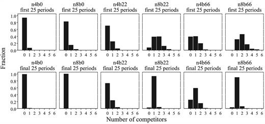
Number of competitors over time. For each treatment, the distribution of the number of players investing in more than two units is displayed, both for the first 25 periods (top row) and for the final 25 periods (bottom row).
More details on how subjects compete are offered in Figure 7, which shows the top three investment levels per group over time. In the treatments without status rents, there are usually two or three subjects investing two units. This illustrates that in these treatments subjects are not able to coordinate on a fixed star network. The picture is different in treatment n4b22, where after some time on average only one subject consistently invests two units and a stable star network is formed. In treatments n4b66 and n8b22 we observe higher investments by the top contributor than in n4b22: the subject in the core learns that an efficient level of four units is needed to prevent being challenged by periphery players. Once it has become clear who is the superstar in a group, the investments by the other group members gradually fade out.21
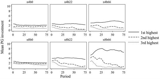
Ranked mean investments. For each treatment the average investments are displayed as a function of time. The top (middle/bottom) line presents the average highest (second/third highest) investment level in the group. Lines are smoothed by taking the moving average over periods t − 5 to t + 5 for every period t.
The most interesting dynamics are observed in treatment n8b66. At the start of the experiment, the mean investments for the second highest contributor are almost as sizable as for the top contributor: on average they invest in 4.00 units in the first 25 periods. Only after a while does this challenger start to give up. To further investigate what is going on in this treatment, Figure 8 provides a more detailed view. Here, we show the top-3 investments across periods in each of the six groups in n8b66.22 In all groups, we see that in early periods at least two players compete for the core position by investing in very high amounts. At some point all but one player give in and a superstar forms with a core player who (over)invests in 7 or 8 units. At these levels, payoffs are to a large extent equalized and periphery players stop challenging the core player.
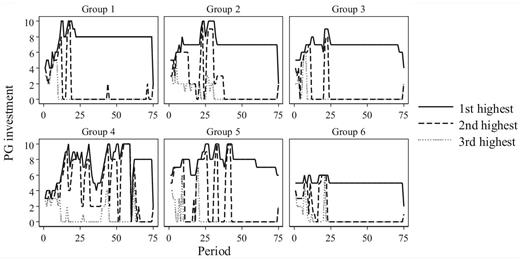
Ranked investments in n8b66. For each group in treatment n8b66 the top-3 highest investments in the group are displayed over time. The top (middle/bottom) line presents the average highest (second/third highest) investment level in the group.
To investigate the stability of the networks formed, Table 7 shows the frequency of various stars and how often they were repeated, after having been formed. The outcomes predicted based on challenge-freeness are listed in bold. In agreement with this concept, star networks occur only sporadically in the treatments without status rents, and if they occur, they tend to be unstable. In n4b22, the predicted 2-star is the most frequently observed and also most stable outcome. In treatments n4b66 and n8b22, the efficient 4-star is predicted to occur, and indeed it is most often observed in both treatments. In these treatments the efficient star is very stable. If it is formed, it remains unchanged in 90% of the cases. Finally in n8b66 a star network is predicted in which the superstar invests in 8 units. Here, in the experiment most often superstars are observed where the core invests in 7 or 8 units, and these outcomes are again remarkably stable. In 88% of the cases in which such a superstar is formed, it is exactly repeated in the next period.
Frequency of periphery-sponsored stars and their stability.
| n4b0 | n8b0 | n4b22 | n8b22 | n4b66 | n8b66 | |
|---|---|---|---|---|---|---|
| 0-star | 5 (0.00) | 3 (0.00) | ||||
| 1-star | 6 (0.00) | 2 (0.00) | 2 (0.00) | |||
| 2-star | 43 (0.21) | 28 (0.50) | 268 (0.65) | 1 (0.00) | 9 (0.56) | |
| 3-star | 1 (0.00) | 67 (0.25) | 67 (0.82) | 59 (0.66) | ||
| 4-star | 8 (0.38) | 151 (0.85) | 172 (0.94) | |||
| 5-star | 7 (0.00) | 15 (0.60) | 47 (0.81) | |||
| 6-star | 1 (0.00) | 9 (0.33) | ||||
| 7-star | 1 (0.00) | 108 (0.92) | ||||
| 8-star | 91 (0.85) | |||||
| 9-star | 2 (0.50) | |||||
| 10-star | 2 (0.00) | |||||
| Other | 545 (0.03) | 417 (0.00) | 255 (0.21) | 233 (0.21) | 344 (0.38) | 191 (0.01) |
| Groups | 8 | 6 | 8 | 6 | 8 | 6 |
| Obs. | 600 | 450 | 600 | 450 | 600 | 450 |
Notes: Cells denote the frequency of the outcomes denoted in the first column across all periods. The proportion of periods that exactly the same strategy profile is played in the subsequent period is given in parentheses. Entries in bold denote the outcomes that are challenge-free.
Finally, we investigate what happens if a core player in a y*-star deviates by lowering her investment. As already noted, y*-stars are very stable: core players rarely lower their investments: of the 319 y*-stars that are formed up to period 65, only 12 core players deviate by lowering their investment.23 This strongly suggest that subjects anticipate that lowering their investment is costly, as they could be challenged and lose the attractive core position. Given the small number of core players who deviate, it is hard to make strong claims about the resulting payoffs, but still we illustrate what subjects might expect in Figure 9. Here we plot the normalized earnings of core players in y*-stars and we split them by whether they lower their investment (at period t = 0) or not. As expected, the core players who lower their investment earn a higher immediate payoff (at period t = 0), but on average pay the price in subsequent periods. These losses outweigh the short-term gains: the aggregated (normalized) losses in periods t = 1 to t = 10 are roughly 7 times the size of the normalized gains at t = 0.
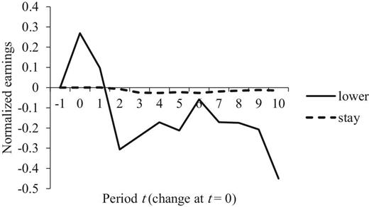
Payoffs from lowering investments as a core player. Mean payoffs of core players in y*-stars. Earnings are normalized by normalizing the payoff in y*-star that is formed at t = −1 to 0. The figure is based on y*-stars where |${y^*} > \hat{y}$|, to ensure that core-players can deviate by lowering their investment.
This result is reminiscent of findings in the Industrial Organization literature on contestable markets. Theoretically and experimentally, it has been shown that monopolistic incumbents can successfully be disciplined to price competitively by the threat of hit-and-run entry by potential rivals. Such hit-and-run behavior is, of course, not exactly the same as challenging in our model, but the idea that central players (in this case monopolists) have to avoid that other players can challenge their position has the same flavor. Baumol et al. (1977) and Panzar and Willig (1977) developed the theoretical argument that an incumbent monopolist satisfies demand in such a way that it remains unprofitable for a potential rival to enter the market. Coursey et al. (1984) provide experimental support for the contestable market hypothesis in the absence of sunk costs.
6.3. Motives Underlying Investments in the Public Good
The evidence presented so far is consistent with the explanation based on a competition for status rents. Once the core position becomes more attractive than the periphery position because of the status rents that it generates, subjects start to challenge it. To prevent being challenged, star players are forced to invest to such an extent that the payoffs across positions are approximately equalized. In this way, status rents are dissipated. However, we cannot exclude that the results are driven by social preferences that do not depend on the possibility to challenge. For instance, subjects may be inequity averse, and therefore choose higher investments to compensate others for the gains that status rents bring. Inequity aversion may also explain why subjects prefer to avoid the core position if it is relatively unattractive in the absence of status rents. Another possibility is that core players feel that they have to return the favor if they receive status rents, or that they are simply driven by altruism and prefer to give something to others as their wealth increases. To investigate the extent to which the possibility of competition for favorable positions is essential, we included the two treatments in which we impose the networks that were naturally formed in the corresponding treatments with endogenous network formation. If challenging of favorable positions drives the results, we should not observe higher investments in these control treatments than the individually rational number of two units.
Table 8 displays the mean, median and predicted public good investments by core players in star networks in the exogenous treatments, together with the benchmarks provided by the endogenous treatments. The results provide convincing support for the concept of challenge-freeness. The results are particularly strong for the case where group size is small and status rents are large; here, the mean and the median are exactly at two units as predicted. Even more so, there are almost no cases where the core player invests in more than two units of the public good. But also in the case with large group size and large status rents, the results are striking: average investment is only a fraction of the level that is achieved when networks are endogenously formed. The differences between the investments in the endogenous and exogenous network treatments are significant at the 5% level.
Mean core-investments in exogenous and endogenous networks.
| Exogenous networks | Endogenous networks | ||||||
|---|---|---|---|---|---|---|---|
| Predicted | Mean (s.e.) | Median | Predicted | Mean (s.e.) | Median | p-value | |
| n = 4 | 2 | 2.00 (0.05) | 2 | 4 | 3.61 (0.18) | 3.5 | 0.028 |
| n = 8 | 2 | 2.85 (0.41) | 2 | 8 | 7.07 (0.45) | 7.5 | 0.028 |
| Exogenous networks | Endogenous networks | ||||||
|---|---|---|---|---|---|---|---|
| Predicted | Mean (s.e.) | Median | Predicted | Mean (s.e.) | Median | p-value | |
| n = 4 | 2 | 2.00 (0.05) | 2 | 4 | 3.61 (0.18) | 3.5 | 0.028 |
| n = 8 | 2 | 2.85 (0.41) | 2 | 8 | 7.07 (0.45) | 7.5 | 0.028 |
Notes: The table lists the predicted, mean, and median investments by core players in the public good, conditional on a periphery-sponsored star being formed. Standard errors of the mean are presented in parentheses, based on taking the mean of the mean investments per group. The median is obtained by taking the median within each group first and then the median within each treatment. The p-values come from 2-sided Wilcoxon signed-rank tests, where we test the null-hypothesis that investments by the core are the same across treatments, conditional on a periphery-sponsored star having formed. Each pair of endogenous and exogenous groups constitutes one individual observation.
Figure 10 shows the distribution of investment choices by core players for each of the treatments with b = 66, both for endogenous and exogenous networks. It is clear that with exogenous networks, core players invest substantially less than with endogenous networks. In both n4b66EXO and n8b66EXO, in periphery-sponsored stars the modal core investment is the stage-game Nash amount of two units, whereas we hardly ever observe such low investments with endogenous networks. An alternative explanation would be that endogenous network formation allows selection of socially motivated types to the core position. Our data provide little support for this selection effect of competition. If it were to hold, one would expect to see these supergame effects in at least 1 out of n exogenous groups. Indeed, in n8b66EXO, we observe some cases where core players invest in more than two units, but these only account for a small number of cases. Moreover, even in these groups investments remain well below the level of 7 or 8 units that we frequently observe in the endogenous network treatments. Hence, such traces of social motives are negligible compared to the competition effect of endogenizing network formation.
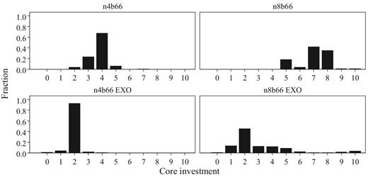
Distribution of core-investments in endogenous and exogenous networks. The figure shows the distributions of investment of core players in treatments with b = 66, conditional on a periphery-sponsored star having formed. All period/group observations are included.
Notice that this evidence underlines the importance of the possibility to compete endogenously for favorable positions. It does not preclude the existence of more complicated social preferences that depend on how the network is shaped. In the presence of status rents, for instance, players might feel the necessity to reciprocate when they benefit from the intentional creation of a valuable link, whereas such a motive is absent when the network is exogenous.24 Though we cannot exclude such complex motivations, we favor the parsimonious explanation that selfish players compete for favorable positions and that the advantaged player behaves in a way to avoid being challenged by others.
7. Conclusion
We have investigated the effects of status rents on the shape and stability of networks and on the level of public good provision. For this, we introduced status rents for incoming links to the endogenous network formation game of Galeotti and Goyal (2010). Our conjecture was that players would jockey to obtain attractive network positions by challenging the position of those with the highest payoffs. In the presence of status rents, this implies that players would compete for status and the winner of the competition for status would be forced to take the interests of the other group members into account. The simple concept of challenge-freeness predicts when a subgame perfect equilibrium outcome is to be expected, and if so, which equilibrium is selected. We subsequently tested these predictions in a laboratory experiment, where we varied group size and status rents across treatments. These are two factors that should systematically affect the equilibrium that is selected if people compete for status rents. Thereby, these factors determine the extent to which the public good is provided and the shape and stability of the outcome.
We find that the presence of status rents is crucial for the results. With status rents, subjects start by jockeying for the core position. Once the dust has settled and subjects have implicitly agreed on who will be in the core of the network, a stable outcome arises in which the core player consistently contributes an amount that roughly equalizes payoffs across positions. This ensures that her position cannot successfully be challenged. For specific environments, this entails contributing more than the stage-game Nash quantity and in some even more than what is efficient. In this way, the core player in a superstar prevents being challenged by the others, and periphery players maintain their links, which the superstar-core needs for her exemplary behavior. As a consequence, status rents are dissipated. Across treatments, we observe that these supergame effects—that is, the adjustment of contributions aimed at maintaining the network (core) position—increase with the size of the status rents and with group size. In stark contrast, inefficiency reigns and groups rarely converge to equilibria when there are no status rents. These experimental results correspond closely to the concept of challenge-freeness and the selection of a subgame perfect equilibrium (if any) that it entails.
With the help of our two control treatments in which we imposed exogenous networks, we excluded the possibility that supergame effects might arise without competition for status rents. In agreement with our conjecture, the observed supergame effects largely disappear when the possibility to compete for the core position is excluded by design. Instead, if our core players in superstars had been driven by other motivations, like altruism or inequity aversion, results should have been independent of how the positions in the network are assigned.
We therefore conclude that free competition for a favorable position is the key ingredient for the emergence of superstars in our environment. Beyond the specific setting of our experiment, this may help explain why so often a small minority in a group contributes so heavily to a public good. There is no need to assume that pure altruism or other prosocial motivations drive this behavior. Even purely self-interested individuals may do so if they care enough about the status rents that are closely linked to being at the core of the group in this way. In short, volunteers at sports teams, workshop organizers and OSS developers all contribute much more to their group than can be expected in a one-shot environment because the supergame they are involved in allows them to collect status rents from the central position that they have.
Acknowledgments
We thank Vincent Buskens, Eric van Damme, Sanjeev Goyal, Matthew Jackson, Jérôme Hergueux, Debraj Ray, Giorgia Romagnoli, Joel Sobel, Juuso Välimäki, and two anonymous referees of this journal for their helpful suggestions. Financial support from the Research Priority Area Behavioral Economics of the University of Amsterdam and of the ANR - Labex IAST is gratefully acknowledged. This paper supersedes our working paper “Superstars Need Social Benefits: An Experiment on Network Formation” (van Leeuwen et al. 2013).
Notes
The editor in charge of this paper was Juuso Välimäki.
Footnotes
We use the term “supergame effect” to describe an increase in the provision of the public good when the stage game is repeated across multiple rounds.
In the working paper that this paper supersedes (van Leeuwen et al. 2013), we considered four treatments that differed in many respects from the treatments reported here. For example, in the previous paper we had no treatments where subjects contributed more than the efficient amount. Based on the previous results, we formulated the predictions—how network stability and the core player's contribution are determined by the relative profitability of the core position—before we ran any of the sessions reported in this paper.
For an overview of the theoretical literature on network formation, see for example Goyal (2007) or Jackson (2008). In a recent study, Kinateder and Merlino (2017) theoretically investigate the role of heterogeneity in the GG framework. They find that the type of heterogeneity affects the set of equilibrium networks and that a version of the law of the few is still present with heterogeneous players. Other theoretical papers that study public good provision on endogenously formed networks include Cho (2010) and Cabrales et al. (2011). Galeotti et al. (2010), Boncinelli and Pin (2012), and Bramoullé et al. (2014) study public good provision on exogenous networks.
The authors attribute these latter results to difference between the GG-model and their laboratory implementation. In their experiment, subjects make repeated decisions, but only the decisions at a random termination moment matter for payment.
Other papers that experimentally study public goods on exogenous networks include Fatas et al. (2010), Carpenter et al. (2012), and Leibbrandt et al. (2015). Eckel et al. (2010) study public good provision on fixed star networks and assign the core positions in some treatments to either “high-status” or “low-status” individuals. Status is determined by performance on a trivia quiz. High-status core players are more often mimicked by the periphery than low-status core players. Several other experimental papers that allow for endogenous network formation (e.g., Ule 2005; Corbae and Duffy 2008; Knigge and Buskens 2010; Berninghaus et al. 2012; Wang et al. 2012) use games that differ substantially from ours.
This, and the following results carry over from GG. As we study a slightly modified game with discrete investments and one-way flow, we provide the proofs in Appendix A for completeness.
As we will describe in Section 5, the Nash star is the only type of stage-game Nash equilibrium in our experiments.
From here onward, we only consider this (arguably most interesting) case where |$c\hat{y} > k$|. If the reverse holds, the unique Nash equilibrium is the empty network (i.e., no links are formed) where all players invest in |$\hat{y}$| units.
Appendices D–F are available in the Online Supplementary Material.
In these auctions, bidders agree on the desirability of distinct positions for their online ads. The ith best position is awarded to the ith highest ranked bidder at a price equal to the (i + 1)th highest bid. The game allows for an extremely large set of equilibria. Edelman et al. (2007) propose the concept of local envy-freeness to select the most plausible equilibrium. In this equilibrium, no player can improve her payoff by exchanging bids with the player ranked one position above her. Varian (2007) provides an empirical analysis of Google auctions and finds that local envy-freeness describes the basic properties of the ad auctions reasonably well.
We include the last inequality of the definition to make the concept portable to other classes of games. In the games considered here, a player who is challenged will always be worse off than without the challenge. In other games, it may happen that a player who is challenged is better off after the challenge. In such cases, we think that the player with the highest earnings wants to be challenged. Thus, it is natural that the strategy profile is not challenge-free if the top-earner is better off after being challenged.
In a previous version of this paper, we provided a dynamic model where players have limited foresight that selects a challenge-free outcome for our experimental games. This version is available on http://www.borisvanleeuwen.nl/superstars_nov16.pdf
To stay close to the GG-model, we let subjects make both decisions simultaneously. An interesting alternative would be to implement a version of the game where players first decide on contributions and only make their linking decisions after the contribution decisions have been communicated. Our conjecture is that a sequential structure would further facilitate the convergence to challenge-free equilibria.
In Appendix C, we provide a table with the payoffs in different star networks for our parameters.
For our experiment, we deliberately chose the values of n and b such that we keep (n − 2)b—and thus y*—constant between treatments n8b22 and n4b66.
In this case, a player earns 42 points.
In treatment n4b66 two groups converged to networks where multiple players invest. In treatment n8b22, one group converged to a situation where 6 out of 8 players formed a periphery-sponsored star, where the core invested in 3 units and the periphery did not invest. Between the other two players, one player invested and the other did not and the latter formed a link to the former.
Details are available upon request.
In this treatment (n4b22), the only two groups that are not classified as stable, also formed periphery-sponsored stars with a fixed core for a substantial number of periods where the core alternated between investing two and three units.
In a regression, we find a negative correlation between risk aversion and being in the core of a star in treatments where we expect competition (i.e., when networks are formed endogenously and b > 0). We find no significant correlation between risk aversion and core positions in the other treatments. Moreover, we do not find any relation between gender and network positions. Similar results are obtained when we use public good investments as the dependent variable. More details are available upon request.
A similar figure of the other treatments is available upon request.
We focus on treatments where |${y^*} > \hat{y}$|, to ensure that core-players can deviate by lowering their investment.
In a similar vein, in the absence of status rents core player might resent free riders who could themselves take up the role of the center, but not those who are exogenously given a position in the periphery.
In the very unusual case where the core earns less than the periphery in the proposed star, no outcome will be challenge-free.
The testable prediction of our model is that an equilibrium is selected that implements a challenge-free outcome-path. A challenge-free outcome path realizes a challenge-free outcome in every stage of the finitely repeated game, except in a final phase where play reverts to a stage game equilibrium. There are typically multiple ways in which this outcome-path can be supported in equilibrium. For instance, in one equilibrium a deviation from a challenge-free outcome is punished by the deviation to an equilibrium where one of the periphery players takes over the profitable core position, and all other players link to this new core player in each subsequent stage, except in the final phase of the finitely repeated game where play reverts to a stage game equilibrium.
Appendix A: Stage-game Equilibria and Efficient
Outcomes
This appendix is greatly indebted to the analysis in Galeotti and Goyal (2010). In agreement with the theoretical literature on network formation, we will restrict our attention to pure-strategy equilibria.
Some Additional Notation.
Most of the notation is introduced in Section 3 of the main text, but for the proofs we will use the following additional definitions. The marginal benefit of accessing the mth unit of the good is given by MB (m) = f(m) − f(m − 1).
A network is a core-periphery network if there are two sets of players |${\what{N}_C}$| and |${\what{N}_P}$| for which it holds that |${N_i}( {{\boldsymbol g}} ) = {\what{N}_C}\backslash \{ i \},\ \forall \ i \in {\what{N}_C}$| and |${N_j}( {{\boldsymbol g}} ) = {\what{N}_C},\ \forall \ j \in {\what{N}_P}$|. In such a network, the players in |${\what{N}_C}$| form the core and |${\what{N}_P}$| form the periphery. All core players form links to the other core players, but not to the periphery players and any periphery player links to all the core players but to none of the other periphery players. A core-periphery network with a single player in the core is called a star network.
Nash Equilibria of the Stage Game.
We start by stating our variant of Lemma 1 in Galeotti and Goyal (2010):
In any Nash equilibriumsN, all players i ∈ N access at least|$\hat{y}$|units of the good, |$y_i^N \ge \hat{y}$|, and all players who acquire units personally will access exactly|$\hat{y}$|units of the good, that is, if|$x_i^N > 0$|then|$y_i^N = \hat{y}$|.
Proof. Suppose that a player i ∈ N accesses fewer than |$\hat{y}$| units of the good, that is, |${y_i} < \hat{y}$|. If this is the case i can strictly increase her payoff by investing as the marginal benefits strictly exceed the marginal costs for |$\le \hat{y}$|, that is, |$MB( m ) > c,\ \forall \ m \le \hat{y}$|. If a player i invests in units personally, that is, xi > 0, and she accesses more than |$\hat{y}$| units of the good, |${y_i} > \hat{y}$|, she can strictly increase her payoff by lowering xi as |$MB( m )\!<\!{c,\ \forall \ m}\!> \hat{y}$|.
Next, we can state our version of Galeotti and Goyal's Proposition 2.
In any strict Nash equilibriumsN, (i) a core-periphery network is formed where (ii) the core players all invest, (iii) the periphery players do not invest, (iv) aggregate investment equals|$\hat{y}$| units, and (v) the maximum number of players in the core is independent of n and b and is given by the largest integer smaller than|$\frac{{c\hat{y}}}{k}$|.
Proof. We start by showing that in every strict Nash equilibrium sN, |$\mathop \sum \nolimits_{i \in N} x_i^N = \hat{y}$| should hold. It is easy to see that by Lemma A.1, it must be that aggregate investment in sN equals at least |$\hat{y}$| units, that is, |$\mathop \sum \nolimits_{i \in N} x_i^N \ge \hat{y}$|. We define the set of all players with incoming links by |${\what{N}_1} = \ \{ i:{\omega _i} > 0\}$| and all players without incoming links by |${\what{N}_0} = \ \{ {j:\ {\omega _j} = \ 0} \}$|. Note that in a strict equilibrium, any player |$i \in {\what{N}_1}$| should invest in strictly more units than any player |$j \in {\what{N}_0}$|. If not, players that link to i could (weakly) improve by moving their links to j. Also, |$cx_i^N > k$| should hold for all |$i \in {\what{N}_1}$|, as otherwise no player would link to i (but rather invest personally), hence |$x_i^N > {k}/{c},\ \forall \ i \in {\what{N}_1}$|. Note that |$\mathop \sum \nolimits_{i \in {{\what{N}}_1}} x_i^N < \hat{y}$| cannot hold, as then for every |$i \in {\what{N}_1}$|, |$y_i^N < \hat{y}$| follows and this contradicts Lemma A.1. We will now show that |$\mathop \sum \nolimits_{i \in {{\what{N}}_1}} x_i^N > \hat{y}$| cannot hold in a strict equilibrium. Assume that it holds. This implies that any |$i \in {\what{N}_1}$| does not link to all other players in N1 as otherwise |$y_i^N > \hat{y}$| follows which contradicts Lemma A.1. Hence, for every |$i \in {\what{N}_1}$|, there exists some |$\ell \ne i \in {\hat N_1}$|, for whom |${g}$|i,ℓ = 0. Without loss of generality we can order the players in |${\what{N}_1}$|such that |$x_1^N \ge x_2^N \ge \cdots \ge x_m^N > {k}/{c}$| holds. As we are considering strict equilibria, this means that no |$i \in {\what{N}_1}$|will link to the last player m in the sequence, as otherwise i could (weakly) improve by linking to someone higher in the sequence. Aggregate investment by all players |$i \in {\what{N}_1}\backslash \{ m \}$| should still be at least |$\hat{y}$| units, as by Lemma 1 |$y_i^N = \hat{y},\ \forall \ i \in {\what{N}_1}$| should hold. This means that there exists some subset |$\what{N}_1^{\prime} \subseteq {\what{N}_1}\backslash \{ m \}$|, whose investments add up exactly to |$\hat{y}$|: |$\mathop \sum \nolimits_{i \in N_i^{\prime}} x_i^N = \hat{y}$|. Take the smallest possible subset |$\what{N}_1^{\prime}$| for which |$\mathop \sum \nolimits_{i \in \what{N}_1^{\prime}} x_i^N = \hat{y}$| holds. Then, as |$x_i^N > {k}/{c},\ \forall \ i \in {\what{N}_1}$|, player m could strictly improve by not investing and linking to all |$i \in \what{N}_1^{\prime}$|. This contradicts m being in |${\what{N}_1}$|in an equilibrium. Hence, it cannot be that |$\mathop \sum \nolimits_{i \in {{\what{N}}_1}} x_i^N > \hat{y}$| and it follows that |$\mathop \sum \nolimits_{i \in {{\what{N}}_1}} x_i^N = \hat{y}$|.
If |$\mathop \sum \nolimits_{i \in {{\what{N}}_1}} x_i^N = \hat{y}$|, this implies that any |$j \in {\what{N}_0}$| will have |$x_j^N = \ 0$|, as they can access |$\hat{y}$| units (at lower costs than investing personally) by linking to all |$i \in {\what{N}_1}$|. Thus aggregate investment equals |$\hat{y}$| and sN must be a core-periphery network where all players |$i \in {\what{N}_1}$| form the core and all |$j \in {\what{N}_0}$| form the periphery. Recall, that |$x_i^N > {k}/{c},\ \forall \ i \in {\what{N}_1}$| holds. As |$\mathop \sum \nolimits_{i \in N} x_i^N = \hat{y}$|, this provides an upper bound for the number of players that invest personally, and hence the size of the core: |$| {{{\what{N}}_1}} | < {{c\hat{y}}}/{k}$|.
Efficient Outcomes.
In any efficient outcome, it must be that aggregate investment is at least |$\hat{y}$| units, that is, |$\mathop \sum \nolimits_{i \in N} {x_i} \ge \hat{y}$|. If not, all players will access fewer than |$\hat{y}$| units and they can strictly increase their payoff (and hence the sum of payoffs) by investing in additional units as |$MB( m ) > c,\ \forall \ m \le \hat{y}$|. As |$c\hat{y} > k$|, the aggregate costs of accessing at least |$\hat{y}$| units of the good are minimized by forming a periphery-sponsored star where only the core invests, that is, |${x_i} \ge \hat{y},\ \ {x_j} = 0,\ \ { g_{j,i}} = 1,\ \ { g_{\ell ,j}} = 0,\ { g_{i,j}} = \ 0, \forall \ j \ne i,\ell \ne i,j$|. The efficient level of investment |${x_i} = \tilde{y}$| by the core is such that the sum of all marginal benefits just exceeds the marginal costs of investing. That is, |$\tilde{y}$| is set such that it satisfies |$nMB( {\tilde{y}} ) \ge c$| and |$nMB( {\tilde{y} + 1} ) < c$|.
Appendix B: Challenge-Free Outcomes
In this appendix we provide proof for Propositions 3.
Section 3.3 of the main text defines the concept of challenge-freeness. In this appendix we derive which networks, if any, are challenge-free. We start with characterizing the set of challenge-free outcomes for general parameters.
If status rents are sufficiently high, that is, when the core earns more than a player in the periphery in the Nash star, the only challenge-free outcome is a star where the core player invests in|${x_c} = \max ( {\hat{y},{y^{\rm{*}}}} ){\rm{\ }}$|and the periphery players do not invest.
If status rents are low, that is, when the core earns less than a player in the periphery in the Nash star, there is no challenge-free outcome.
Proof. Case 1 considers part (i) and case 2 considers part (ii). In both cases, we order the players by their payoffs: Π1(s) ≥ Π2(s) ≥ |$\cdots$| ≥ Πn−1(s) ≥ Πn(s).
Case 1: |$( {n - 1} )b \ge c\hat{y} - k$|. For this case we show that the only challenge-free outcome is a star where the core player invests in |${x_c} = \max ( {\hat{y},{y^{\rm{*}}}} )$| and the periphery players do not invest. For most parameters, including the parameters used in all of our experimental treatments, the core will earn more than the periphery in the proposed star and is therefore (by definition) player 1.25 Note that by the definition of y* (see Section 3.3), the periphery will not challenge the core. Moreover, if players in the periphery invest anything or make any other links than to the core, they can improve their payoff by reducing their investment to zero and removing the superfluous links. This means that no network other than a star can be challenge-free. Hence, if any network is challenge-free, it must be the proposed star network. To establish that this network is indeed challenge-free, we show that if player 1 (the core) deviates from the proposed strategy, she will either be challenged or obtain a lower payoff.
First suppose that player 1 uses a strategy with investment x1 < y*. In this case, any player i > 1 can (and will) challenge player 1 by investing slightly more, that is,|${\rm{\ \ }}x_i^{\prime} = \max ( {{x_1} + 1,\hat{y}} )$|, and not forming any links. This follows directly from the definition of y* and equation (2) in Section 3.3 of the main text. Another possibility is that player 1 uses a strategy with investment x1 > y* and |${y^{\rm{*}}} \ge \hat{y}$|. In this case, player 1 can strictly improve her payoff by reducing her investment to |$x_1^{\prime} = {y^{*}}$| without being challenged. Finally, if x1 ≥ y* and |${y^{\rm{*}}} < \hat{y}$|, player 1 can strictly improve her payoff by changing her investment to |$x_1^{\prime} = \hat{y}$| without being challenged. If player 1 forms any links she can strictly do better by removing them.
Case 2:|$( {n - 1} )b < c\hat{y} - k$|. Section 3.3 of the main text shows that Nash stars and superstars are not challenge-free in this case. In Nash stars and superstars, core players challenge by lowering investment (to 0) and linking to one of the periphery players, in the expectation that the latter will invest |$\hat{y}$|. We will now show that all other networks are also not challenge-free.
Suppose that player 1 invests |${x_1} \ge \hat{y}$|. If player i > 1 challenges player 1, she invests 0 and forms a link to player 1, expecting a payoff of Πi(s′) = f(x1) − k. For the network to be challenge-free, it must be that this challenge is unprofitable to i : Πi(s) ≥ Πi (s′) = f(x1) − k. As Π1(s) ≥ Πi(s) by construction, it must also be that Π1(s) ≥ f(x1) − k. Note however that—following Assumption 1—player 1’s payoff is at most Π1(s) ≤ f(x1) − cx1 + (n − 1)b, which contradicts Π1(s) ≥ f(x1) − k for the case we are considering. Hence, this outcome cannot be challenge-free.
Now consider the possibility in which |$0 \le {x_1} < \hat{y}$|. Notice that because of Assumption 1, any player i > 1 will not link to 1 in a challenge-free outcome. If i would have a link to player 1, she prefers to challenge player 1 and withdraw her link to player 1. This means that player 1 is isolated and earns less than the payoff that she would obtain by investing |${x_1} = \hat{y}$|. As Π1(s) ≥ Πi(s), player i can then always challenge by investing |${x_i} = \hat{y}$| and forming no links. Hence, any such network cannot be challenge-free.
Predictions for the Experiment.
All treatments with status rents and endogenous network formation fall in Case 1. In these treatments, |${y^*} \ge \hat{y}$| and the y*-star is the unique challenge-free outcome, which we take as the prediction for those treatments.26 The treatments without status rents (n4b0 and n8b0) fall in Case 2. In these treatments there is no challenge-free outcome and we predict no stable outcomes.
Appendix C: Additional Tables
Payoffs and welfare in different star networks.
| n4b0 | n8b0 | n4b22 | n8b22 | n4b66 | n8b66 | ||||||||
|---|---|---|---|---|---|---|---|---|---|---|---|---|---|
| Core inv. | πP | πC | W | πC | W | πC | W | πC | W | πC | W | πC | W |
| xC = 1 | 22 | 37 | 103 | 37 | 191 | 103 | 169 | 191 | 345 | 235 | 301 | 499 | 653 |
| xC = 2 | 82 | 42 | 288 | 42 | 616 | 108 | 354 | 196 | 770 | 240 | 486 | 504 | 1078 |
| xC = 3 | 107 | 12 | 333 | 12 | 761 | 78 | 399 | 166 | 915 | 210 | 531 | 474 | 1223 |
| xC = 4 | 126 | −24 | 354 | −24 | 858 | 42 | 420 | 130 | 1012 | 174 | 552 | 438 | 1320 |
| xC = 5 | 129 | −76 | 311 | −76 | 827 | −10 | 377 | 78 | 981 | 122 | 509 | 386 | 1289 |
| xC = 6 | 132 | −128 | 268 | −128 | 796 | −62 | 334 | 26 | 950 | 70 | 466 | 334 | 1258 |
| xC = 7 | 133 | −182 | 217 | −182 | 749 | −116 | 283 | −28 | 903 | 16 | 415 | 280 | 1211 |
| xC = 8 | 134 | −236 | 166 | −236 | 702 | −170 | 232 | −82 | 856 | −38 | 364 | 226 | 1164 |
| xC = 9 | 135 | −290 | 115 | −290 | 655 | −224 | 181 | −136 | 809 | −92 | 313 | 172 | 1117 |
| xC = 10 | 136 | −344 | 64 | −344 | 608 | −278 | 130 | −190 | 762 | −146 | 262 | 118 | 1070 |
Notes: Payoffs for core (πC) and periphery (πP) players in different star networks where the periphery players do not invest. W denotes the welfare level, which is defined as the sum of payoffs.
MW tests for differences in the relative frequencies in periphery-sponsored stars in the final 25 periods.
| Treatment | n4b0 | n8b0 | n4b22 | n8b22 | n4b66 | n8b66 |
|---|---|---|---|---|---|---|
| n4b0 | – | |||||
| n8b0 | 0.49 | – | ||||
| n4b22 | 0.00 | 0.00 | – | |||
| n8b22 | 0.02 | 0.02 | 0.29 | – | ||
| n4b66 | 0.04 | 0.08 | 0.07 | 0.51 | – | |
| n8b66 | 0.00 | 0.00 | 0.50 | 0.53 | 0.28 | – |
| Treatment | n4b0 | n8b0 | n4b22 | n8b22 | n4b66 | n8b66 |
|---|---|---|---|---|---|---|
| n4b0 | – | |||||
| n8b0 | 0.49 | – | ||||
| n4b22 | 0.00 | 0.00 | – | |||
| n8b22 | 0.02 | 0.02 | 0.29 | – | ||
| n4b66 | 0.04 | 0.08 | 0.07 | 0.51 | – | |
| n8b66 | 0.00 | 0.00 | 0.50 | 0.53 | 0.28 | – |
Notes: Entries are p-values coming from Mann–Whitney tests using group averages as the independent unit of observation.
