


Abstract
The correct prediction of how alternative states of the world affect our lives is a cornerstone of economics. We study how accurate people are in predicting their future well-being after facing major life events. Based on individual panel data, we compare people’s life satisfaction forecasts reported in the first interview after a major life event with their actual evaluations five years later on. This is done after the individuals experience widowhood, unemployment, disability, marriage, separation, or divorce. We find systematic prediction errors that seem at least partly driven by unforeseen adaptation after the first four of these events.
1. Introduction
When people form predictions about their future well-being, not only do they have to consider the possible states of the world they might live in, but they also have to anticipate the tastes or preferences that will impact their (hedonic) experiences. To ensure utility maximizing decision making in this context, neoclassical utility theory relies on two fundamental assumptions: First, people, on average, correctly estimate the probabilities of possible decision outcomes. Second, they know their preferences and the extent to which these might change. If these assumptions do not hold, people are unable to form correct expectations about the utility that they will derive from alternative situations. They are then likely to make suboptimal decisions, which will, in turn, lead to lower levels of individual welfare compared to a situation with unbiased expectations. Importantly from the perspective of economics, this would undermine the validity of inferring preferences from observed behavior (see Loewenstein et al. 2003; Kahneman and Thaler 2006; Frey and Stutzer 2014 for general accounts of utility misprediction).
In this paper, we study how successful people are at making predictions about the development of their future utility approximated by subjective well-being in response to major life events. We deviate from the rational expectation paradigm and allow prediction errors in expected outcomes as well as in expected preferences. As one possible source of prediction errors, the emphasis is on adaptation as a form of endogenous change in preferences. The term adaptation signifies that an individual’s emotional and evaluative response to a given change in circumstances diminishes over time. Using data on life satisfaction, recent studies show that many life events do not lead to permanent shifts in satisfaction levels, suggesting that people tend to adapt to various changes in life circumstances (e.g., Clark et al. 2008; Oswald and Powdthavee 2008; or recently, Clark and Georgellis 2013). However, it remains a challenge to assess how accurately people predict their adjustment to new life circumstances.
The standard procedure used to identify forecasting errors is to compare predictions with direct measures of experienced well-being: People are asked to predict how they would feel within a certain time period subsequent to a future event. The participants’ responses are then compared with their or other respondents’ actual feelings after experiencing the event. Such studies are part of research on affective forecasting in psychology (see, e.g., Wilson and Gilbert 2003 or for a review from an economic perspective Loewenstein and Schkade 1999). One prevalent finding of such studies is that people tend to systematically overestimate the degree to which they will be affected by an event.1 However, there are two main challenges that research designs have to address in order to be able to identify people’s hedonic mispredictions. First, there is the risk of spurious forecast errors resulting from selection. To address this challenge, one can compare the predictions and realizations for the same individuals. However, this is no trivial task with events that are hard to foresee, for example, widowhood. Second, when generating data on people’s forecasts, questions regarding particular events have to be asked, rendering the event in question salient, which could in turn potentially contribute to prediction errors (Levine et al. 2012, 2013).
The present study applies large-scale long-run panel data on predicted satisfaction with life in order to identify prediction errors after major life events. We transfer the idea of using evaluative subjective well-being as a proxy for current utility to predicted subjective well-being as a proxy for expected future utility. In order to study people’s ability to accurately predict their future satisfaction level in response to major life events, we make use of the German Socio-Economic Panel (SOEP). In this annual survey, participants are not only asked about their individual life satisfaction, but also about how satisfied they expect to be in five years time. Both questions ask for general evaluations, which allows us to test the accuracy of people’s predictions regarding the long-term impact of life changes without referring specifically to the event. In particular, the data track the survey participants’ evaluations of actual life satisfaction as well as their predictions about their future life satisfaction around the event in question. This allows us to compare the expected and the actual long-term consequences after an event. In total, we use data from 14 survey waves from 1991 until 2004, consisting of over 180,000 person–year observations. The scope of this panel data allows us to use a within-subject (fixed effects) approach to measure potential prediction errors in people’s everyday lives.
We extend the identification strategy applied in the literature so far, which captures the development of satisfaction patterns around life changes. Specifically, we estimate two distinct patterns. The first pattern shows the impact of the event on individuals’ actual satisfaction, and the second pattern shows the impact of the event on the predicted satisfaction. In doing so, we can compare changes in predicted satisfaction in the first interview after the event with the actual changes in life satisfaction five years later. A potential error in this case simply captures the difference between the predicted long-term impact of the event and the actual impact of the event. By looking at the adjustment process, we can show whether and to what extent life events increase prediction errors, and thereby statistically abstract from other sources of prediction errors, in particular individual-specific and age-specific effects. By focusing on the predictions made in the first interview after the event, we are able to study to what extent people fail to anticipate the degree to which they will adjust to recently experienced changes in life circumstances. With widowhood, unemployment, and disability we consider three life shocks in the domains of social relationships, the labor market, and health, respectively. Further, we study three major life decisions, namely, marriage, separation, and divorce. Considering positive and negative events allows us to study potential asymmetries.
The main results show substantial systematic prediction errors for some events, with the discrepancy between predicted and reported satisfaction being greatest with regard to widowhood. In the latter case, people, on average, underestimate their future life satisfaction by 0.634 points on an eleven-point scale. This means that they are overly pessimistic regarding their recovery from widowhood measured by their life satisfaction. The estimates indicate that people are also unduly pessimistic about their future level of satisfaction after experiencing unemployment or disability. Furthermore, focusing on plant closure as an exogenous event for individual job loss provides evidence against the concern that the prediction errors of newly unemployed individuals are driven by a self-selection of overly pessimistic people into unemployment. For marriage, the results suggest that people, on average, tend to be overly optimistic about their satisfaction in five year time. We study the robustness of the results regarding the use of different samples that indicates that our results cannot be explained by sample attrition or sample selection over time. With regard to separation and divorce, the estimated differences are sensitive to such alternative sample definitions and lend no support to the existence of a systematic error in one direction.
The identified prediction errors for widowhood, unemployment, disability, and marriage potentially comprise errors that are driven by biased beliefs about future changes in circumstances, as well as by unanticipated adaptation. With regard to widowhood, for example, people might underpredict the level of satisfaction experienced five years hence, because they underestimate the probability of finding a new partner or because adaptation is stronger than anticipated. In an attempt to discriminate between these two different sources of prediction errors, we focus on individuals who remain in the respective status for at least five years. By focusing on individuals who remain in the unfavorable status of widowhood, unemployment, or disability, we can in principle exclude any underestimation of life satisfaction in five years time that is due to overly pessimistic beliefs about future changes in the respective status. For marriage, the opposite applies. Individuals who remain widowed or disabled show prediction errors in the same direction and similar in size to the results of the analysis using the full sample. This provides first evidence that the errors are at least partly driven by unforeseen adaptation.
Beside the misprediction of circumstances and the underestimation of adaptation, there might well be alternative and complementary explanations and underlying (psychological) mechanisms for the observed systematic prediction errors. First, we highlight the challenge of empirically discriminating between systematic changes in the use of the satisfaction scale and true hedonic adaptation. In order to address the issue empirically, we conduct an empirical test that makes use of people’s retrospective evaluations of their life satisfaction for the year prior to the interview. Second, we include a discussion of the possibility that the two life satisfaction questions are anchored. If anchoring represents a true mental process, that is, that people systematically expect future life satisfaction to be similar to current satisfaction, such anchoring could indeed be seen as a psychological mechanism for the prediction bias. It is important though to discriminate between such true mental anchoring and induced anchoring due to the ordering of the questions. Third, we investigate focalism as a possible psychological mechanism underlying the underestimation of adaptation, that is, people are unable to anticipate that the major life event will preoccupy them less in the future and therefore exaggerate its impact on their future satisfaction. Fourth, we address the possibility that people’s answers in the survey are driven by social desirability. Newly widowed, for example, might not feel comfortable reporting to an interviewer that they expect to be more satisfied in five years’ time than in the current situation. Fifth, we discuss the extent to which learning might have a positive impact on the accuracy of people’s predictions and what obstacles might hinder people from learning from experience.
The remainder of the paper is organized as follows: Section 2 offers a brief review of the literature, presents basic theoretical considerations, and the general hypotheses. The data and empirical strategy are described in Section 3. Section 4 presents the estimations of the prediction errors for the life events studied. In Section 5, we focus on the (partial) neglect of adaptation as a potential driver of prediction errors. Section 6 discusses and partly tests alternative mechanisms that could potentially explain our results. Section 7 offers concluding remarks.
2. Previous Evidence and Theoretical Considerations
Forward-looking decisions require the formation of expectations. In the standard economic model, decision makers are assumed to hold objectively correct probabilistic expectations regarding unknown future outcomes. Thus, although agents’ expectations may be wrong because the future is not fully predictable and may entail (news) shocks, they are never systematically biased given their information set and their understanding of the world.2 In addition, the preferences underlying forecasts about utility are assumed to be stable.
In our analyses and the simple theoretical framework (see Section 2.2), we deviate from this rational expectation paradigm and allow prediction errors in expected outcomes as well as in expected preferences. We thus follow the empirical literature that measures expectations based on self-reports. Although this research concentrates on subjective probabilities for future outcomes (see, e.g., Manski 2004), we want to consider future preferences and overall expected utility as well. In our brief review (see Section 2.1), we concentrate on these latter aspects.
2.1. Previous Evidence
The economic analysis of subjective well-being lends itself to the study of potential prediction errors related to future preferences, as measures of subjective well-being can serve as proxies for individual welfare (Frey and Stutzer 2006, 2014; Kahneman and Thaler 2006; Hsee et al. 2012). Regarding future preferences or the endogenous change in preferences, adaptation is a key process that contributes to it and thus potentially to utility misprediction.
2.1.1. Adaptation
Although it seems self-evident that people’s well-being changes in most instances if circumstances change, it is less clear to what extent such changes persist when the new conditions stabilize. There is a strong scientific claim of hedonic relativism in psychology, that is, that changes in well-being are only temporary (for a discussion, see Sheldon and Lucas 2014, and specifically, Powdthavee and Stutzer 2014). This view is related to the prominent work by Brickman and Campbell (1971), which proposes the idea of a hedonic (or happiness) set point that is regained after a process of adaptation: people get used to a new situation or repeated stimuli and thereby return to their innate level of experienced well-being.
Their conclusions provoked substantial empirical research on adaptation. Thus, it is now standard practice to conduct longitudinal analyses and to study profiles of reported subjective well-being around life events. This allows for individual-specific level effects to be taken into account when exploring adaptation. Empirical studies on adaptation refer to various events such as marriage, widowhood, divorce, birth of a child, separation, unemployment, crime victimization, or disability (see, e.g., Lucas 2007; Clark et al. 2008; Frijters et al. 2011; Clark and Georgellis 2013 for studies involving multiple events, and Luhmann et al. 2012 for a meta-analysis). Overall, the evidence suggests that there is adaptation to changes in circumstances due to major life events. This adaptation, however, differs across events and is far from complete for some of them.
The interpretation of estimated profiles relies on at least two assumptions. First, it is assumed that reported subjective well-being can be analyzed as a cardinal measure. An early study by Ferrer-i-Carbonell and Frijters (2004) comparing cardinal and ordinal analyses of reported life satisfaction on an eleven point scale showed little difference in their statistical findings when the inherently ordinal nature of the data was neglected. A second assumption is that there is no rescaling; that is, people self-assign the same score on the subjective well-being scale for a given level of perceived satisfaction with life over the course of a life event. This crucial assumption is rarely made explicit in previous work. We discuss it in our context in more detail in Section 6.1.3
2.1.2. Affective Forecasting and Projection Bias
Given the evidence that people to some extent adapt to changing circumstances with respect to subjective well-being, the question arises whether such adaptation is anticipated or not. We investigate this question in what follows by studying the accuracy of people’s predictions after major life events. Previous evidence reports that individuals are not good at foreseeing how much utility they will derive from possible future conditions of the world (for a review, see Wilson and Gilbert 2003 and recently Wilson and Gilbert 2013). Research on affective forecasting shows, in particular, that people tend to overestimate their reactions to specific events, because they are embedded within other daily life events that they are not consciously aware of. Another reason for errors in predicting emotions is that people underestimate their ability to successfully cope with negative events. The phenomenon that people are generally unaware of the influence their psychological immune system has in reducing negative affect is known as immune neglect in the psychological literature (e.g., Gilbert et al. 1998). This mechanism works in complementarity with the tendency to overrate the impact of any single factor. Kahneman et al. (2006) refer to the latter tendency as focusing illusion. The general notion is that people have biased expectations about the intensity and duration of their emotional responses, in the sense that the emotional impact is often less harsh than predicted, because people adapt to the new circumstances more easily than they anticipate. This general idea has been productively modeled and introduced in economics as projection bias (Loewenstein et al. 2003).
The general idea of an impact or projection bias has been well received. However, its conceptual explanation, which is based on focalism, that is, “the tendency to focus on one event and neglect to consider how emotion will be mitigated by the surrounding context” (Lench et al. 2011: 278), has been the source of important methodological criticism of the literature and of typical study designs. When people are asked about their forecasts regarding specific aspects of their future status, a focus or salience is induced that might itself create a bias in affective forecasting. Specifically, even when people are asked to predict their general well-being, their response might indicate how they expect to feel about the respective status (see the discussion between Levine et al. 2012, 2013 and Wilson and Gilbert 2013). We discuss the problem of induced salience in more detail in Section 6.3.
2.1.3. Predicted Satisfaction with Life
In our approach, we draw on forecasts that do not ask about expected satisfaction with specific circumstances. Instead, we consider people’s general predictions of their future life satisfaction. In a longitudinal study, these assessments can then be compared with current reported life satisfaction when the time arrives. Frijters et al. (2009) apply this approach in studying the accuracy of forecasts in East Germany after the fall of the Berlin Wall, but before reunification, and find evidence of clear initial overoptimism. In their rich empirical analysis, they further find that the aggregate prediction errors fell substantially within roughly five years. Moreover, the level of overoptimism was lower for people with higher levels of education, but higher for those living on the border or moving to the West-German states. Based on the same panel data for Germany, Lang et al. (2013) and Schwandt (2016) document a systematic life-cycle pattern where young people have overly optimistic expectations about their future life satisfaction, whereas older people gradually become overly pessimistic about their future well-being. Schwandt argues that this pattern in unmet expectations partly drives the U-shape in the relationship between age and well-being. Although these studies put their primary focus on the evolution of aggregated prediction errors, we aim to identify prediction errors in the context of individual life events.
2.2. Theoretical Framework and Hypotheses
We analyze the argument of potentially systematic prediction errors in individual well-being within a setting of state-dependent utility, inspired by the framework of projection bias in Loewenstein et al. (2003). The general hypothesis is that people’s predictions of their future instantaneous utility tend to be biased toward the current state of preferences, as they do not fully anticipate changes in their tastes, for example, due to adaptation. However, in our generalized framework of prediction errors, people might not only systematically err in terms of changes in preferences (or future tastes) but also in terms of changes in circumstances. In our setting, changes between current and future circumstances are reflected by changes in people’s statuses, for example, from the status of being unemployed to being employed or from being married to being separated. Our framework emphasizes that potential errors in predicting both preferences and future circumstances (i.e., status changes) need to be considered in empirical tests.
Hypotheses about the direction of errors in forecasts of future subjective well-being after life changes, however, are difficult to formulate. Integrated predictions of future preferences and future circumstances might involve potentially countervailing sources of error. With regard to preference changes or adaptation, we rely on the general claim in the literature that people tend to neglect these aspects when forming their predictions (implying α > 0). Given the previous evidence that at least some adaptation is associated with the major life events that we study, we expect the following: people are overly optimistic with regard to their future life satisfaction after marriage and are overly pessimistic after becoming separated, divorced, widowed, unemployed or disabled.
However, the overall prediction errors may be different if people’s predictions of circumstances are systematically wrong. This may be the case because they systematically misperceive the probability of a status change. There is indeed evidence for an optimism bias; that is, an overestimation of the likelihood of positive events (see, e.g., Sharot 2011 for a review). Newly weds might underestimate the risk of divorce, thus supporting an overestimation of future life satisfaction. In contrast, unemployed people might overestimate their re-employment prospects, thereby counteracting overly pessimistic forecasts of their well-being (or even transforming the latter into overly optimistic forecasts).
In the empirical analyses in Section 4, we test these hypotheses by investigating the average prediction errors for people who forecast their well-being after major life events. Comparable to the idea of a reduced form approach, this strategy allows capturing the net prediction error that comprises potentially different sources. In Section 5, we make a first attempt in order to discriminate between the two basic sources of prediction errors mentioned, that is, unanticipated adaptation and misperceived future circumstances. We propose a test that evaluates the possibility of a prediction error for a subsample of individuals who experience the event. For this subsample, the goal is to exclude as many systematic prediction errors as possible regarding future life circumstances. Any remaining misprediction of the adjustment process after major life events will then most likely be ascribable to a prediction error regarding future preferences.
3. Data and Empirical Strategy
3.1. Data Description
Our empirical analysis is based on individual-level panel data from the SOEP, an extensive representative survey of the population in Germany (Wagner et al. 2007). Since 1984, SOEP has surveyed the German population and asked a wide range of questions regarding their socioeconomic status and their demographic characteristics. In the survey, subjective well-being is reported by answering the question: “How satisfied are you with your life, all things considered?”. In some years, people are subsequently asked “And how do you think you will feel in five years?”. For both questions, respondents are asked to respond via a scale that ranges from 0, meaning “completely dissatisfied”, to 10, meaning “completely satisfied”. The first question was asked every year, and over fourteen consecutive years, between 1991 and 2004, both questions were asked in the survey. The item nonresponse is less than half a percent for current satisfaction and less than two percent for predicted satisfaction. The resulting data on the two key variables provide the information used in this study to investigate potential prediction errors.
We focus our analysis on six major life events. This includes three negative life shocks, that is, widowhood, unemployment and disability and three life decisions, that is, marriage, separation, and divorce. As indicators for the events, we follow the strategy presented in Clark et al. (2008) and use the year-to-year changes of the respective statuses for each individual. For example, the first time the marital status of an individual changes to widowed indicates the first observation after the event of widowhood or the status change. The same strategy applies for marriage, separation and divorce. All status changes are self-reported. People are classified as separated when they report that they are married but live (permanently) separated from their spouse. This involves people who report their status change at the residents’ registration office (involving a change in their tax class) as well as informally separated people. For unemployment, the status change to registered unemployment is decisive. Disability is defined on the basis of a scale that indexes its severity. It captures the legally attested reduction in earning capacity from 0 to 100. We categorize an individual as being disabled when the index crosses the threshold value of 30. This is the minimum level for being potentially put on a par with a severely handicapped person.
In our baseline analysis, we only consider an event if the corresponding status change occurs within the sample period for an individual. Hence, we exclude respondents for whom we have no observation indicating the point in time when they changed their status (left-censored spells), as we are consequently unable to calculate how long they have been, for example, widowed. We further require a full record of observations without missing years. This assures that we observe all status changes. We concentrate on the first status change we observe in the survey period for each individual. For the labor market-related events of unemployment and disability, we further restrict the sample to individuals under the age of 60 who are not about to retire within the next five years. This prevents expectations about retirement from systematically influencing predicted life satisfaction. Apart from only including respondents who are older than 16 years of age, we have no further age restrictions for widowhood, marriage, separation, and divorce. For disability, information on the status of individuals is not available for 1993. Therefore, we impute the information of the following year if a legally attested disability is indicated in the year before and after 1993. We exclude the 102 cases for which this information is not given.
We restrict the sample to the period from 1991 to 2004 and use the same sample across the two key satisfaction measures. This allows us to study the impact of the life shocks and life decisions on people’s actual and predicted life satisfaction, given the same macroeconomic circumstances. We further require nonmissing observations for all variables. In our analyses, we include both people who have experienced the status change in question and those who are not in the respective status, but who might experience a transition to it. Including people who are at risk of experiencing an event in question allows us to estimate the coefficients of our control variables more precisely. In particular, this strategy allows us to estimate the profile of life satisfaction around life events vis-à-vis a counterfactual situation of general changes in circumstances. This is particularly important for time-specific effects that otherwise might be difficult to separate from the impact of the life events themselves.
Table 1 provides a summary of the number of observations for individuals who experience widowhood, unemployment, disability, marriage, separation, or divorce for the corresponding years before and after the event. As noted, observations are included irrespective of whether an individual changes his or her status again, as for example, when the individual finds a new job after becoming unemployed.4 The uneven number of observations in the years just before and after the event and the decreasing number of observations in the years following the event derive from missing values in any of the variables, panel attrition, and age- and year-specific sample restrictions. Descriptive statistics are presented in Table A.1 of the Appendix, exemplifying for the sample generated to study the effect of widowhood. All characteristics listed will serve as control variables in the respective analysis. The restrictions leave us with a final sample of 183,532 observations for the analysis of widowhood, 143,190 for unemployment, 143,045 for disability, 64,547 for marriage, 190,990 for separation, and 187,085 for divorce. Depending on the specification and the event studied, people remain in the sample, on average, for 5.4 to 7.0 years. Robustness tests regarding the selection of the sample and panel attrition are considered in Section 4.4. The relatively low number of observations for marriage derives from the restriction to people who can potentially marry. We thus exclude those individuals who are already married when they are surveyed the first time. This applies to more than 60% of the sampled individuals.
Number of observations before and after the events.
| Widowhood | Unemployment | Disability | Marriage | Separation | Divorce | |
|---|---|---|---|---|---|---|
| Before the event | ||||||
| 3 years and more | 4,173 | 8,731 | 6,996 | 6,025 | 3,050 | 3,916 |
| 3–2 years | 550 | 2,253 | 968 | 1,320 | 603 | 608 |
| 2–1 years | 591 | 2,680 | 998 | 1,579 | 651 | 615 |
| 1–0 years | 606 | 3,146 | 1,039 | 1,822 | 698 | 575 |
| After the event | ||||||
| 0–1 years | 564 | 3,226 | 1,000 | 1,768 | 672 | 539 |
| 1–2 years | 521 | 2,968 | 831 | 1,604 | 614 | 479 |
| 2–3 years | 468 | 2,474 | 706 | 1,467 | 534 | 417 |
| 3–4 years | 417 | 2,142 | 594 | 1,306 | 471 | 364 |
| 4–5 years | 365 | 1,835 | 515 | 1,205 | 414 | 324 |
| 5–6 years | 358 | 1,742 | 431 | 1,041 | 397 | 303 |
| 6 years or more | 1,771 | 8,646 | 1,736 | 4,949 | 1,822 | 1,339 |
| Total | 10,384 | 39,843 | 15,814 | 24,086 | 9,926 | 9,479 |
Source: SOEP.
3.2. Descriptive Evidence
For descriptive evidence, Figure 1 plots the development of actual mean life satisfaction and mean predicted life satisfaction around the status changes. People who become widowed are, on average, pessimistic about their life prospects. This is revealed by predicted levels of life satisfaction being lower than current levels of life satisfaction in the years prior to the event. Given that the average widowed person is relatively old, this observation is consistent with previous findings that older people tend to be pessimistic regarding their future life satisfaction (Schwandt 2016).5 In the first interview after experiencing the event, these same people tend to be slightly optimistic. However, they are not optimistic enough in the year zero, if their prediction of a life satisfaction of 5.80 for year five is compared with their actual life satisfaction of 6.84 five years after the event. Predicted and actual life satisfaction seem closer in the case of unemployment and disability when the prediction in year zero and the realization in year five are compared. Around marriage, separation, and divorce, people are optimistic regarding their future life satisfaction. The high expectations right after marriage are clearly not borne out by the slightly declining pattern in actual life satisfaction. For separation and divorce, however, people’s optimism is to some extent in line with the increasing life satisfaction people experience on average after the event. For all the events, we observe that the impact of the event on predicted satisfaction is weaker in general than it is on actual satisfaction. This suggests that people expect the impact of the event to fade out, but only partially.6
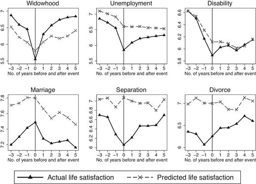
Patterns in mean actual and predicted life satisfaction around life events. Sample sizes are presented in Table 1. Source: SOEP.
3.3. Empirical Strategy
A descriptive analysis based on raw discrepancies between actual and predicted life satisfaction has clear limitations, as individuals who experience an event might share underlying sociodemographic characteristics related, for example, to overly pessimistic predictions. Moreover, individual-specific differences in optimism or pessimism might drive the dispersion of errors. Such aspects of selection and heterogeneity need to be taken into account in order to properly identify prediction errors regarding the adjustment process after major life events. We do this and extend the established identification strategy applied when the development of satisfaction patterns around life changes is studied. In this latter research, separate time dummies for the years around the events are used to capture the effects of these life changes on subjective well-being before and after the individual’s status changes. This allows us to estimate the patterns shown in Figure 1 in a panel regression framework.
Our strategy comprises three steps. In a first step, we estimate the pattern of the impact of an event on the predicted satisfaction in five years. The average impact of an event at the time of the first observation after it occurred then includes the anticipated adjustment. In other words, it reflects the expectations regarding the long-term impact of the event. If people believe that they will return to their old satisfaction level within five years, the event should in turn not affect predicted satisfaction. In a second step, we estimate the actual changes in life satisfaction around the event following the strategy used in other studies. The estimations show how satisfaction changes around major life events. We thus estimate the full pattern of an event’s impact, particularly for the period five years after the event. In a third step, the expected average change can then be compared with the actual impact of an event five years after its occurrence. This provides us with a direct measure of the prediction error associated with the events, conditional on the average individual-specific errors in the period prior to the three years preceding the event.
The two equations only differ in terms of the dependent variable. PSit stands for the predicted life satisfaction of individual i at time t, and LSit stands for the realized actual life satisfaction of individual i at time t. Xit is a vector of individual controls.
The main variables of interest are a series of dummy variables E|$^{j}_{\mathit it}$| indicating the number of years j before and after a specific event. The first dummy E|$^{-3}_{\mathit it}$| captures observations two to three years before the event. The last dummy captures the reports of people who experienced the event six or more years previously. This means that all the years preceding this three-year period prior to the event form the reference level. Importantly, we further include individual fixed-effects αi. This controls for any time-invariant characteristics, and implies that the partial correlations are only based on variation within the same person over time. It thus rules out that stable individual-specific optimism or pessimism drives the differences between predicted and experienced life satisfaction. Still, the control strategy is not sufficiently restrictive if such optimism or pessimism is not constant over time, because, for example, older people become pessimistic. Therefore, the vector of control variables includes age-specific fixed effects that capture changes in our dependent variables that are common for a particular age group. Time-fixed effects are further included to control for systematic changes over time that are common to all the individuals. Region-fixed effects control for regional characteristics that might be correlated with our variables of interest. Standard errors are clustered at the individual level. This takes into account that idiosyncratic errors εit might be serially correlated and standard errors, in turn, understated (Bertrand et al. 2004).
The difference θ|$_{0}^{PS}$|– θ|$_{5}^{LS}$| reflects the average change in individual prediction errors due to an event. A statistically significant difference (rejection of H0) provides support for the hypothesis that people mispredict their long-run life satisfaction changes after the respective event, conditional on the average individual-specific errors four years or more before the status change. The identifying assumptions are (i) that reported (predicted) life satisfaction can be cardinally interpreted, (ii) that people’s interpretations of the scales do not change due to the event, and (iii) that there are no systematic effects of the status change in the data preceding the three-year period prior to the event. This latter condition is necessary to ensure that the average prediction error of an individual in the period preceding this three-year period prior to the event can serve as a valid counterfactual.
4. Average Prediction Errors Following Life Events
4.1. Life Shocks: Widowhood, Unemployment, and Disability
Table 2 presents the results for the estimated models outlined in equations (3) and (4) for widowhood, unemployment and disability.8 For all the events, we show the regression results for the two dependent variables side by side. Columns labeled PS indicate estimates with predicted satisfaction as the dependent variable. Columns labeled LS show the estimates with current life satisfaction as the dependent variable. The latter estimates are comparable to the results in the literature that exploring satisfaction profiles around life events.
Predicted (PS) and actual life satisfaction (LS) around four major life shocks.
| Widowhood | Unemployment | Disability | Plant closure | |||||
|---|---|---|---|---|---|---|---|---|
| PS | LS | PS | LS | PS | LS | PS | LS | |
| (1) | (2) | (3) | (4) | (5) | (6) | (7) | (8) | |
| Before event | ||||||||
| 3–2 years hence | −0.020 | −0.088 | 0.004 | −0.042 | −0.034 | −0.048 | 0.029 | 0.119 |
| (0.07) | (0.06) | (0.04) | (0.04) | (0.06) | (0.05) | (0.13) | (0.10) | |
| 2–1 years hence | −0.268*** | −0.308*** | −0.055 | −0.108*** | −0.122** | −0.134** | −0.051 | 0.033 |
| (0.08) | (0.07) | (0.04) | (0.04) | (0.06) | (0.06) | (0.13) | (0.11) | |
| Within the next year | −0.442*** | −0.446*** | −0.123*** | −0.217*** | −0.387*** | −0.536*** | −0.235* | −0.339*** |
| (0.08) | (0.08) | (0.04) | (0.04) | (0.07) | (0.07) | (0.14) | (0.12) | |
| After event | ||||||||
| 0–1 year | –0.617*** | −1.241*** | –0.375*** | −0.818*** | –0.491*** | −0.648*** | –0.630*** | −1.083*** |
| (0.10) | (0.11) | (0.05) | (0.05) | (0.07) | (0.07) | (0.15) | (0.13) | |
| 1–2 years | −0.269*** | −0.481*** | −0.299*** | −0.457*** | −0.374*** | −0.469*** | −0.401** | −0.635*** |
| (0.10) | (0.10) | (0.05) | (0.05) | (0.08) | (0.08) | (0.16) | (0.14) | |
| 2–3 years | 0.005 | −0.201** | −0.250*** | −0.295*** | −0.434*** | −0.462*** | −0.243 | −0.521*** |
| (0.11) | (0.10) | (0.05) | (0.05) | (0.09) | (0.08) | (0.16) | (0.14) | |
| 3–4 years | −0.094 | −0.025 | −0.273*** | −0.219*** | −0.512*** | −0.501*** | −0.282* | −0.241* |
| (0.11) | (0.10) | (0.05) | (0.05) | (0.09) | (0.09) | (0.17) | (0.14) | |
| 4–5 years | −0.018 | 0.037 | −0.348*** | −0.210*** | −0.490*** | −0.401*** | −0.336* | −0.182 |
| (0.12) | (0.11) | (0.06) | (0.05) | (0.10) | (0.10) | (0.17) | (0.14) | |
| 5–6 years | 0.149 | 0.017 | −0.368*** | –0.161*** | −0.341*** | –0.291*** | −0.328* | –0.136 |
| (0.12) | (0.12) | (0.06) | (0.06) | (0.11) | (0.10) | (0.17) | (0.14) | |
| 6 or more years | 0.195* | 0.110 | −0.451*** | −0.168*** | −0.460*** | −0.367*** | −0.651*** | −0.283** |
| (0.11) | (0.11) | (0.06) | (0.06) | (0.10) | (0.10) | (0.16) | (0.14) | |
| Difference: | –0.634*** | –0.214*** | –0.200* | –0.494*** | ||||
| PS (0–1 year)–LS (5–6 years) | (0.12) | (0.06) | (0.10) | (0.17) | ||||
| Alpha-parameter | 0.504*** | 0.326*** | 0.560*** | 0.522*** | ||||
| (0.07) | (0.08) | (0.20) | (0.14) | |||||
| Individual controls | Yes | Yes | Yes | Yes | Yes | Yes | Yes | Yes |
| Age fixed effects (FE) | Yes | Yes | Yes | Yes | Yes | Yes | Yes | Yes |
| Time and region FE | Yes | Yes | Yes | Yes | Yes | Yes | Yes | Yes |
| Individual FE | Yes | Yes | Yes | Yes | Yes | Yes | Yes | Yes |
| No. of observations | 183,532 | 183,532 | 143,190 | 143,190 | 143,045 | 143,045 | 109,084 | 109,084 |
| No. of individuals | 30,978 | 30,978 | 25,233 | 25,233 | 25,366 | 25,366 | 20,738 | 20,738 |
| R2 | 0.04 | 0.04 | 0.03 | 0.03 | 0.04 | 0.04 | 0.03 | 0.03 |
Notes: OLS estimations. Standard errors in parentheses. Alpha-parameter expresses the degree to which the adjustment is not foreseen, calculated based on equation (6). Significance levels: *0.05 < p < 0.1; **0.01 < p < 0.05; ***<0.01; Bold numbers are used in order to highlight the coefficients of primary interest. Source: SOEP.
Column (2) in Table 2 reveals that widowhood has a large negative short-term effect on people’s life satisfaction. Compared to their baseline level of subjective well-being in the time preceding the three-year period prior to the event (i.e., the reference period), reported satisfaction is 1.241 points lower within the first year after the event. It also reveals that the effect fades over time. After three years, the difference is close to zero and no longer statistically significant. This also holds five years after the event. However, the estimation results in column (1) indicate that people, on average, expect their life satisfaction in five years’ time to be substantially negatively affected by the loss of their spouse. The predicted life satisfaction is 0.617 points below the level during the reference period. In the second year, a negative effect for the future is still predicted, though of a smaller magnitude.
Based on the estimates, we have an empirical comparandum to the theoretical prediction error from equation (1). It is the difference that results when the actual impact (the coefficient for 5–6 years in specification (2)) is subtracted from the predicted impact (the coefficient for 0–1 year in specification (1)). We can test the statistical significance of the difference based on the strategy presented in equation (5). In the case of widowhood, the estimates reveal a statistically significant prediction error of −0.634 on the eleven-point satisfaction scale, thus indicating negative expectations that are too pessimistic. The alpha-value of 0.504 suggests that around 50% of the adjustment is not foreseen. This finding is in line with our hypothesis that people underestimate adjustment processes that counteract shocks to subjective well-being.
For the two shocks related to the work realm, unemployment, and disability, prediction errors resulting from overly negative expectations are found, consistent with the main hypothesis. However, these two events differ from the previous one, as people do not fully return to their original satisfaction level, even after 5–6 years. This observation is in line with the literature that reports no full adjustment for individuals who continue to have the same respective status. However, with our sample, we measure the initial as well as the long-term effect of the event for all the people, irrespective of whether they remain disabled or unemployed. The finding from the literature that people do not fully adjust to these two events therefore holds even for a sample that does not exclude people who overcome the adverse condition. Moreover, individuals tend to underpredict the degree to which they will regain their original satisfaction level after being confronted with the negative impact of the events. Regarding unemployment, they underpredict their future satisfaction by −0.214 points, and regarding disability, they underpredict it by −0.200 points. As expressed by the alpha-parameter, the adjustment unforeseen amounts to about 33% in the case of unemployment and 56% in the case of disability.
In order to simplify the interpretation of the regression coefficients provided in Table 2, we present the estimation results graphically in Figure 2. The solid black line shows the effects on current satisfaction, whereas the gray x-marks capture the effects on predicted satisfaction. In order to facilitate the approximation of the prediction error, a dashed black line is included to signify the event’s effect on the predictions right after the event (0–1 year after the event) across the time periods up to period five (5–6 years after the event). The prediction error is thus reflected in the difference between the dotted line and the solid black line in period five.
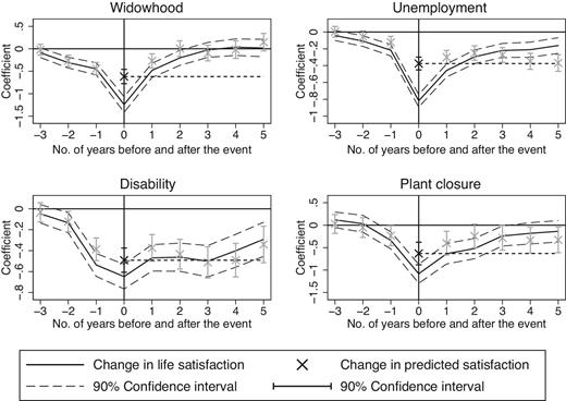
Estimated patterns in actual and predicted satisfaction around four major life shocks. Based on the estimated coefficients in Table 2. The dashed black line is an auxiliary line that indicates the effect of the event on the expected satisfaction five years after the event. The prediction error is reflected in the difference between the dashed black line and the solid black line (capturing the effect on actual satisfaction) in period 5. Source: SOEP.
For the three events, the change in predicted satisfaction closely tracks the change in actual satisfaction, which implies that people do not expect substantial adjustments when they experience a level of life satisfaction that deviates from their level in the reference period. Moreover, the effects of the events on the actual satisfaction levels are generally larger than on the predicted satisfaction levels. This holds in particular for the first observation after the status change (0–1 year after the event). Although individuals thus might anticipate some adjustment, the figures suggest that their predictions for their long-term adjustment are too conservative. This holds even for the short term. Figure 2 shows that the deviations of actual satisfaction from baseline satisfaction level are smaller after only a few periods than they are from the predicted long-term satisfaction level. This is indicated by the solid black line that crosses the dashed black line as soon as after one period in the case of widowhood, and after two periods in the case of unemployment.
4.2. Exogenous Event: Layoff due to Plant Closure
In our estimation approach, we control for the fact that people hold an optimistic or pessimistic outlook to the extent to which we can model it as a stable trait and can capture it with individual fixed effects. Thus, even if the occurrence of events in people’s lives are not independent of how rosy they perceive their future to be, it does not per se pose a problem for our identification strategy.
However, there might be changes in people’s prospects that make them gloomy and affect both their prediction of their future well-being as well as their performance, for example, on the labor market. Thus, if momentarily pessimistic people self-select into unemployment (either voluntarily or due to a dismissal), the negative prediction error for newly unemployed people might reflect a selection effect. To address this, we focus on layoffs caused by plant closures as an exogenous source of unemployment (see Kassenboehmer and Haisken-DeNew 2009 as an application of this strategy in order to measure the effect of unemployment on life satisfaction). In contrast to studying general job loss, we are here able to capture an effect of unemployment on the prediction of future well-being that is closer to a causal interpretation.
For the empirical analysis, we use the same sample as in our main estimation for unemployment previously. However, we additionally restrict it to incidences of unemployment caused by plant closure. As this information is not available for the years 1999 and 2000, we have to exclude people who experience a transition into unemployment during this period. This leaves us with 358 individuals who became unemployed due to plant closure, of which 210 individuals remained in the sample for at least five years.9
Columns (7) and (8) in Table 2 present the estimation results, and the graphic representation of the coefficients is plotted in Figure 2 below the plot of the patterns around general unemployment. What emerges is a picture similar to that in the previous estimates on unemployment in general. Although individuals anticipate some adjustment, they underestimate the degree to which they will regain their initial satisfaction level after being confronted with the negative shock. The alpha-value indicates that 52% of the adjustment is not correctly foreseen. The statistically significant prediction error amounts to 0.494 points. This is more than twice the size of the prediction error estimated for all people who become unemployed, irrespective of the source of their status change. This suggests that for the event of unemployment, the prediction bias cannot be explained by self-selection of overly pessimistic people into unemployment.
4.3. Life Decisions: Marriage, Separation, and Divorce
Table 3 presents the results for marriage, separation, and divorce. Newly wed couples experience a period of life satisfaction above their reference level (coefficients for 0–1 year = 0.345 in specification (2)) and predict this higher level will hold at least partly over time (coefficients for 0–1 year = 0.202 in specification (1)). This evaluation turns out to be overly optimistic, with a life satisfaction score only 0.069 points above the reference level 5–6 years after the wedding. This amounts to a prediction error of 0.134 points, which is statistically significant at the 10% level and implies, with an alpha-value of 0.483, that 48% of the adjustment is not correctly foreseen. For separation and divorce, we do not find a statistically significant prediction error. In the case of separation, people’s prediction of their satisfaction five years later is quite accurate, on average, though with a large standard error. Although life satisfaction drops significantly by 0.598 points on average for people who separate from their partner, they correctly expect that their satisfaction five years later will not significantly differ from their baseline satisfaction level. In the case of divorce, people experience the largest drop in satisfaction in the year before they get divorced. This is not surprising, given the institutional setting in Germany which restricts divorce to those people who have been separated for at least one year. For unilateral divorce, people need to be separated for at least three years. This law makes it difficult to empirically separate the effects for divorce from those for separation. In particular, the low level of life satisfaction in the year before the divorce is likely to be driven by the negative circumstances related to separation. Due to this institutional feature, the reference period for the estimation of the coefficients around divorce might be confounded with anticipation effects of separation. We therefore include an additional lead effect (4–3 years hence) in specifications (5) and (6). The graphic representation of the coefficients are shown in Figure 3.
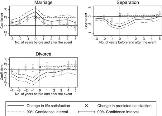
Estimated patterns in actual and predicted satisfaction around three major life decisions. Based on the estimated coefficients in Table 3. The dashed black line is an auxiliary line that indicates the effect of the event on the expected satisfaction five years after the event. The prediction error is reflected in the difference between the dashed black line and the solid black line (capturing the effect on actual satisfaction) in period 5. Source: SOEP.
Predicted (PS) and actual life satisfaction (LS) around three major life decisions.
| Marriage | Separation | Divorce | ||||
|---|---|---|---|---|---|---|
| PS | LS | PS | LS | PS | LS | |
| (1) | (2) | (3) | (4) | (5) | (6) | |
| Before event | ||||||
| 4–3 years hence | −0.072 | −0.186*** | ||||
| (0.07) | (0.07) | |||||
| 3–2 years hence | 0.071* | 0.068 | −0.126* | −0.109* | −0.081 | −0.347*** |
| (0.04) | (0.04) | (0.07) | (0.06) | (0.08) | (0.08) | |
| 2–1 years hence | 0.073 | 0.120** | −0.071 | −0.134* | 0.077 | −0.365*** |
| (0.05) | (0.05) | (0.08) | (0.07) | (0.08) | (0.08) | |
| Within the next year | 0.174*** | 0.245*** | −0.245*** | −0.485*** | 0.050 | −0.507*** |
| (0.05) | (0.05) | (0.08) | (0.08) | (0.09) | (0.09) | |
| After event | ||||||
| 0–1 year | 0.202*** | 0.345*** | 0.045 | −0.598*** | 0.104 | −0.266*** |
| (0.05) | (0.06) | (0.09) | (0.09) | (0.09) | (0.09) | |
| 1–2 years | 0.093* | 0.153*** | 0.040 | −0.413*** | 0.118 | −0.116 |
| (0.06) | (0.06) | (0.09) | (0.09) | (0.09) | (0.09) | |
| 2–3 years | 0.013 | 0.100 | 0.008 | −0.166* | −0.056 | −0.145 |
| (0.06) | (0.06) | (0.09) | (0.09) | (0.11) | (0.10) | |
| 3–4 years | 0.104 | 0.128* | 0.051 | −0.206** | −0.047 | −0.062 |
| (0.07) | (0.07) | (0.10) | (0.09) | (0.11) | (0.11) | |
| 4–5 years | 0.063 | 0.145** | −0.075 | −0.149 | 0.163 | 0.037 |
| (0.07) | (0.07) | (0.10) | (0.10) | (0.11) | (0.11) | |
| 5–6 years | −0.009 | 0.069 | 0.133 | –0.001 | 0.155 | –0.035 |
| (0.08) | (0.08) | (0.10) | (0.10) | (0.12) | (0.12) | |
| 6 or more years | −0.038 | −0.018 | 0.085 | −0.023 | 0.188 | 0.161 |
| (0.08) | (0.08) | (0.10) | (0.10) | (0.12) | (0.11) | |
| Difference: | 0.134* | 0.046 | 0.139 | |||
| PS (0–1 year)–LS (5–6 years) | (0.08) | (0.12) | (0.13) | |||
| Alpha-parameter | 0.483** | |||||
| (0.20) | ||||||
| Individual controls | Yes | Yes | Yes | Yes | Yes | Yes |
| Age fixed effects (FE) | Yes | Yes | Yes | Yes | Yes | Yes |
| Time and region FE | Yes | Yes | Yes | Yes | Yes | Yes |
| Individual FE | Yes | Yes | Yes | Yes | Yes | Yes |
| No. of observations | 64,547 | 64,547 | 190,990 | 190,990 | 187,085 | 187,085 |
| No. of individuals | 12,063 | 12,063 | 32,349 | 32,349 | 31,663 | 31,663 |
| R2 | 0.03 | 0.04 | 0.04 | 0.04 | 0.04 | 0.04 |
Notes: OLS estimations. Standard errors in parentheses. Significance levels: *0.05 < p < 0.1; **0.01 < p < 0.05; ***<0.01; Bold numbers are used in order to highlight the coefficients of primary interest. Source: SOEP.
4.4. Robustness Regarding Alternative Samples
We assess the robustness of our results for the prediction of adjustment in subjective well-being with regard to three alternative sample selections and re-estimate the specifications in Tables 2 and 3 accordingly. First, we address concerns regarding attrition in our baseline sample, as some people leave the sample between the first and the sixth period after the event. For these people, we only observe a prediction of their life satisfaction without its corresponding realization. If panel drop-outs are systematically related to how people are affected by an event, the estimated prediction errors are potentially affected by panel attrition. For example, someone could be severely affected by a negative event and, in turn, might correctly predict low future satisfaction. If such a person is more likely to drop out, the prediction might look too bleak compared with the effect on actual satisfaction for the remaining people five years after the event. This kind of selection effect would lead to a spuriously larger prediction error. Therefore, we also estimate the patterns based on those individuals for whom we have both a prediction of life satisfaction right after the event and a realization five years later, dropping all individuals for whom either the predicted or the respective realization five years later is missing. We are thus able to follow the adjustment process for at least five years for all individuals affected.
The second check takes into account that we do not have observations in the reference period for all individuals affected, that is, in the time period preceding the more than 3 years prior to the event. So far, we have assumed that the people we observe in the reference period are not systematically differently affected by the life events considered than those for whom we do not have observations in the reference period. In order to understand the sensitivity of our results with regard to this assumption, we exclude those people from our analysis for whom we do not have observations in the reference period.
The third robustness check considers an alternative control sample of people who might have experienced an event but did not, selected on the basis of matching. Rather than drawing someone from our database who might change their status, for example, from being employed to being unemployed to form a comparison group, we therefore select only people who are similar to those who have actually experienced an event. This latter group might be more appropriate for capturing the counterfactual evolution of subjective well-being over time, given the circumstances. The matching is based on propensity scores that rely on characteristics of individuals who actually experience the event in question in three years’ time. For the prediction of the propensity scores for the people in the control group, we use people’s first observations in the period from 1989 to 2004, applying nearest neighbor matching (without replacement).
Figure 4 presents a summary of the resulting prediction errors for the baseline samples, as well as the samples generated for the robustness checks. For all the events with the exception of divorce and separation, the prediction errors derived from the robustness checks show the same sign as the ones in the analysis based on the main sample. The effects for widowhood, unemployment, and disability remain similar in size and, except for disability, statistically significant throughout. For marriage, the prediction error is no longer statistically significant in every specification, and approximately a third of the size when only those individuals are considered, for whom the prediction and the realization are observed. The statistically weaker results might not come as a surprise, as the respective estimations rely on fewer observations. In the case of change in marital status from being married to being separated or divorced, prediction errors vary between positive and negative, whereas never being statistically different from zero when estimated on the basis of different samples. Overall, the prediction errors derived from the alternative samples are similar in magnitude for widowhood and unemployment and are aligned in the same direction for disability and marriage. It is thus unlikely that the main findings for these events are the result of a biased reference period or panel attrition.
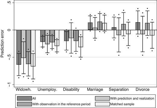
Prediction errors based on alternative samples. Both 90% and 95% confidence intervals are indicated (solid black line and dots, respectively). The prediction errors for all refer to the estimation results in Tables 2 and 3. Prediction errors for With prediction and realization restrict the sample to observations for predictions right after the event that are all matched with the corresponding realizations for the same individuals five years later. Prediction errors for With observation in the reference period restrict the sample to those people for whom we have observations prior to 3 years before the event. Prediction errors for Matched sample restrict the samples to similar people who might still experience the events. The corresponding regression outputs are presented in Section S.5 in the Supplementary Material.
5. Mispredicted Circumstances Versus an Underestimation of Adaptation
Our findings so far reveal systematic prediction errors after major life events. The patterns in reported subjective well-being after the events suggest that the measured prediction errors could be interpreted to some extent to be unanticipated adaptation. However, prediction errors may just as well occur owing to unanticipated changes in circumstances (i.e., status changes).
We conduct a supplementary analysis to shed some light on the two possible sources or explanations for prediction errors in subjective well-being. This inquiry relies on specific subsamples to explore whether a particular selection of people mispredict their subjective well-being because they underestimate their capacity to adapt to the new circumstances. In order to be clear about the underlying sources of prediction errors as well as the strategy behind our supplementary analyses, we extend our theoretical framework in the following Section 5.1 before proceeding with the empirical analysis in Section 5.2.
5.1. An Extended Framework with Two Sources of Prediction Errors
Prediction errors may occur due to unanticipated adaptation as well as due to unanticipated changes in circumstances. The latter occurs, for example, when people who have lost a spouse and thought that they would remain alone unexpectedly find a new partner. Regarding unemployment, people who expect to remain unemployed due to poor job prospects, and who are therefore pessimistic about their future satisfaction, may nevertheless find a new job. In order to conceptually discriminate between changes in circumstances and preferences as two sources of errors in utility predictions, we extend the simple theoretical framework outlined in Section 2.2.
The resulting error consists of three terms. The first term α(Ui(Ci, t, Si, t) – Ui(Ci, t, Si, t+k)) captures the utility differential due to the change in preferences that is weighted by the factor α for the nonanticipation of adaptation. The greater the change in preferences is, and the less this change is anticipated (α > 0), the larger the error (which can be either positive or negative) will be. In the case of unanticipated adaptation to the negative event of unemployment, for example, this term would increase the negative value of the error, and thus reflect underestimated utility. The second term (p΄ – p)Ui(ci, t+k,Si, t+k) picks up the contribution to the error that emerges if the potential change in circumstances is not correctly anticipated. An overestimation of future utility occurs, for instance, in a situation where a newly unemployed person anticipates that he or she has a chance of finding a new job (p΄ >0), but where this positive change in circumstances does not materialize (p = 0). Hence, this term either reduces or increases the prediction error that is due to the individual’s neglect to consider possible adaptation. The third term α p΄(Ui(ci, t+k, Si, t) – Ui(ci, t+k, Si, t+k)) captures another factor that contributes to the prediction error caused by a change in preferences. However, this factor only relates to the change in circumstances, and only to the extent that the change is expected. This latter term captures the correction of the second term to the extent that the two sources of the overall bias interact; that is, where the utility prediction regarding the anticipated change in circumstances was made subject to incorrect beliefs about the future state of preferences.
5.2. Evidence Supporting the Underestimation of Adaptation
Although misprediction due to changes in circumstances and preferences can be easily separated conceptually, the empirical identification of the different components of the error is not straightforward. One would need people’s expectations about changes in their circumstances (i.e., the expected probability of a status change) in order to separate the components empirically. As people’s expectations are not captured in the data, we cannot include such measures in our estimations. However, there is a constellation of circumstances for those people who experience an event that is more likely to capture the prediction error due to adaptation. Specifically, we can focus on individuals who do not experience a change in their status after a life event. For example, the group of widowed people who experience adverse future circumstances as reflected in not finding a new partner within five years after becoming widowed are unlikely to be overly pessimistic when forming expectations about future circumstances (i.e., their future status). If these same people still underestimate future subjective well-being after becoming widowed, then their prediction error is likely to be caused by adaptation that is not fully anticipated. For them, our test can be interpreted as identifying a lower bound for the misprediction of adaptation. Similarly for people who experience the positive life event of becoming married. If the selection of people who we observe remaining married for at least five years and overestimating future subjective well-being after getting married, then they are unlikely to be overly optimistic when forming expectations about their future circumstances. Then their overoptimism is likely to be caused by adaptation that is not fully anticipated.
In the following, we develop this idea more fully in the context of our theoretical framework and test it empirically. The focus is on circumstances that are tied to an individual’s status (i.e., that are associated with the various life events). These circumstances may change after an event in the sense that people either remain in the status that led to a reduction (or a gain) in subjective well-being or leave it. In our framework, statuses change with probability p, and people have to form expectations p΄ about this probability when predicting subjective well-being. Leaving their current status thereby means that they will find a new partner, separate or get divorced, find employment, or regain their health. People who remain in their status (realization of p = 0) therefore consist of those people who have been (a) either correct or too pessimistic regarding their prospects marriage and those who have been (b) either correct or too optimistic regarding favorable status changes after widowhood, unemployment, and disability. If for these same people, prediction errors in subjective well-being show the opposite pattern (i.e., overestimation of future life satisfaction after marriage and underestimation after the negative events), this cannot be explained by an inaccurate expectation of the probability of leaving their respective status. However, unanticipated hedonic adaptation would be a consistent explanation.
As explained in what follows, the test exploits the fact that changes in circumstances related to a specific status are likely to be unidirectional, that is, that for the negative (positive) events the circumstances can primarily improve (worsen). This condition, however, does not hold for separation and divorce. In both of these situations, the relationship status can easily become either better or worse. We therefore concentrate on the other four life events for which we identified significant prediction errors.
The regression analysis of our test is based on the same sample as the one used for the main analysis. However, we estimate separate patterns of actual and predicted life satisfaction for those individuals who leave their status after a life event and for those who remain in their respective status for at least five years. The criterion applied to categorizing individuals as remaining disabled requires that the gravity of their incapacity is evaluated as being above the threshold index of 30, and that the degree of their disability has made no improvement during the first five years after suffering the handicap. Note that the number of observations for the case of disability and especially for that of unemployment is rather small.10
Figure 5 presents the estimation results graphically.11 In the cases of widowhood and disability, even the people who remain in their status underestimate their life satisfaction in five years time. With an error of −0.627 for widowhood, the size is almost identical with the result in Table 2. For disability, the calculated prediction error of −0.323 is even larger than if calculated for everybody who experiences the event. For marriage, the forecasts remain slightly overoptimistic, but the prediction error is smaller and not statistically significant. Overall, the findings suggest that at least in the case of widowhood and disability, the observed average prediction errors are to a large extent driven by the underestimation of adaptation (and not by prediction errors attributable to unanticipated changes in circumstances).12
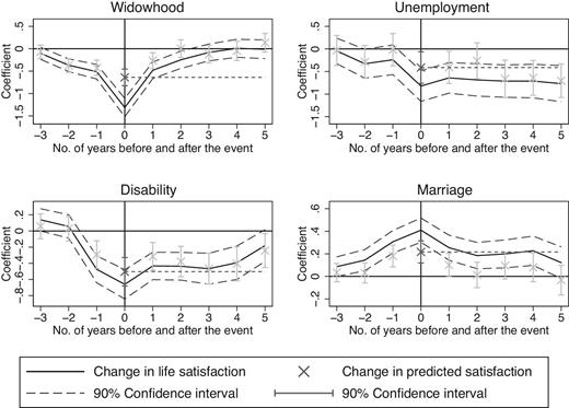
Estimated patterns in actual and predicted satisfaction for those who remain in the status in question for at least 5 years. Based on the estimated coefficients in Table S.5 in the Supplementary Material. The dashed black line is an auxiliary line that indicates the effect of the event on the expected satisfaction five years after the event. The prediction error is reflected in the difference between the dashed black line and the solid black line (capturing the effect on actual satisfaction) in period 5. Source: SOEP.
In the case of unemployment, those individuals who remain unemployed are observed to be too optimistic regarding their future life satisfaction. Due to the small number of individuals who experience long-term unemployment, the effect is, however, imprecisely measured and not significantly different from zero. Since no adaptation is observed in the pattern of life satisfaction for the long-term unemployed, it is logical that no unanticipated adaptation is detected.13
6. Alternative Explanations and Underlying Mechanisms of Prediction Errors
Our empirical approach indicates that people make systematic prediction errors regarding their future subjective well-being after experiencing some life events. So far we have emphasized the misprediction of circumstances and the underestimation of adaptation as possible explanations. Regarding the underestimation of adaptation, different specific psychological mechanisms might play a role that we want to explore in a next step. Moreover, we focus on alternative explanations that would reduce the observed phenomena to statistical artifacts due to people’s response behavior in surveys. In particular, we address the issues of rescaling, anchoring, the focusing illusion, salience, social desirability and learning related to the reporting of current and predicted subjective well-being.
6.1. Rescaling
A key identifying assumption that is used when comparing predicted satisfaction with its realization five years later is that people’s interpretation of the scale does not change over time. If this assumption is violated, the observed changes in life satisfaction after the events might not be driven by true (hedonic) adaptation, but instead by scale changes. These scale changes are discussed in the literature under different terms such as scale norming (Frederick and Loewenstein 1999), response shift (Schwartz and Sprangers 1999), or scale of reference bias (Groot 2000) and often refer to the health context in which people report their subjective health or their experienced pain. The general claim is that individuals do not rate their own situation in reference to an absolute standard, but in reference to a relative standard, and that this relative standard might change over time (e.g., Kievit et al. 2010). However, it remains unclear whether the change in the relative standard is associated with a real change in hedonic experience, that is, true hedonic adaptation, or only with a change in the description of the same hedonic experience, that is, scale norming. With respect to our analysis one might argue that the changes in satisfaction identified after—say—negative life events do not reflect an actual improvement in well-being among respondents, but only result from a change in the application of the scale. In turn, if these changes of scale are not anticipated by the individuals at the time of their prediction, the identified prediction errors reflect unforeseen scale changes instead of unforeseen adaptation.
Although it is a challenge to empirically discriminate scale norming from true (hedonic) adaptation, our estimation approach allows us to account for changes in scales in several ways. As we apply age-fixed effects, scale changes do not contribute to the prediction error if they occur due to changes in age (see, e.g., Groot 2003 for age norming). Scale changes are not a problem if the scale changes between the last interview before the event and the first interview after the event and then remains constant over time, because we do not use pre-event predictions to estimate the prediction error. In such a case, the same scale is applied for the prediction and the realization, as both of these judgments are formed after the event. However, if people systematically change the way they use the scale over the five years between prediction and realization, and if this scale change is not foreseen, the estimated prediction error would at least partially reflect rescaling. Thus, our identifying assumption—narrowly specified—is that the response scale remains constant between the first interview after the event when the prediction is made and the interview five years later when we measure the actual realization of subjective well-being. Otherwise, we could not compare the prediction and the realization of life satisfaction in order to identify prediction errors, as they would not be based on the same scale.
In order to investigate whether rescaling is a potential explanation for the observed adjustment in subjective well-being after life events, we make use of retrospective evaluations in the SOEP. In our empirical test presented in Section S.7 in the Supplementary Material, we do not find any evidence of systematic scale changes. We conduct the test for the four events widowhood, unemployment, disability, and marriage, for which we find significant prediction errors in the main analysis. In brief, the test makes use of people’s retrospective evaluations of their life satisfaction for the year prior to the interview. When people assess their current satisfaction as well as the satisfaction one year ago in the same point in time, we can presume that they apply the same internal standard for the evaluation of both states. Any differences between the actual reported satisfaction one year in the past and the re-evaluated satisfaction for this period could either be driven by a biased memory or by a change in scale interpretation. However, in our analyses, we do not find significant differences between the evaluations for widowhood and unemployment. This provides some evidence that the scale people apply does not change in the years after the event. For disability and marriage, no systematic adjustment after the event is observed for the subsample at hand. Therefore, we cannot apply the test to these life events in a straightforward way. The results of the test provide no empirical evidence that the identified misprediction in the main analysis is driven by scale changes.
6.2. Anchoring
Another explanation for the occurrence of prediction errors could lie in the ordering of the two well-being questions in the survey. The order is always the same, with the question about predicted satisfaction being asked after the question about current life satisfaction. Given this sequence, people might anchor the answer they gave on to the question about predicted satisfaction to their answer about current life satisfaction. If people systematically expect future life satisfaction to be similar to current life satisfaction, this kind of anchoring could be interpreted as being a myopic forecast that represents a true mental process that drives our effect. However, instead of reflecting on their true expectations, the ordering of the questions could also induce people to arrive at their answer to the predicted satisfaction question “on the fly” by anchoring it to the question about current life satisfaction (Kahneman 1999, p. 22). Anchoring of this latter kind might lead to a prediction error after a life event that is conditioned by the survey design.
However, if the prediction errors identified in our main analysis were only an artifact induced by the ordering of questions, we would expect the prediction errors to be present and symmetric for all life events for which we observe an impact on life satisfaction. The findings of only a small prediction error after people get married and the nonsystematic errors after separation and divorce, do not provide evidence supporting this claim. Thus, although anchoring might well be part of the mental process that leads to the underestimation of adaptation, it is at least not deterministic and does not provide a conclusive explanation for our results.
6.3. Focusing Illusion and Salience
When people predict their subjective well-being after a major life event, they may well neglect to consider that they will think less about the event in the future and therefore overestimate the impact of the event on their satisfaction. This focalism or focusing illusion (Schkade and Kahneman 1998) can be seen as one potential mechanism that prompts the underestimation of adaptation. If people neglect to consider that the strength of their emotional response to an event will diminish as the event becomes less salient over time, their judgments will act as a complementary driver of overrating the long-term consequences of a life event. However, it is important to distinguish between a focusing illusion or true hedonic salience and situations where the questions (or question contexts) induce salience by referring to the life events in question when people formulate their predictions about future satisfaction. Salience provoked by the question context might induce prediction errors, even if the satisfaction judgment is elicited without a reference to the life event. This is the content of the criticism formulated by Levine et al. (2012, 2013) regarding some of the research on the impact bias in affective forecasting.
Based on the dataset at hand, it is not possible to directly study the relevance of salience, as people are not specifically asked to reflect on experienced life events. However, there is one aspect of the survey, that is, changes in the ordering of particular questions in the SOEP, that allows us to get close to a test of salience. In the years 1994, 1995, 2000, 2003, and 2004, people were asked whether they had experienced a change in their family situation just before they were asked about their current and predicted satisfaction with life. In other years, there was at least one buffer question between the life satisfaction questions and the one asking about changes in the family. We exploit these differences in the ordering of the questions in order to study whether and to what extent making the family-related life events salient has an influence on predicted life satisfaction. We include a detailed description of the test and the results in Section S.8 in the Supplementary Material. In brief, we do not find statistically significant differential changes of predicted life satisfaction for the group for whom the life event is made salient in the questionnaire. This provides some evidence that the measured prediction errors are not simply an artifact of the survey context. Of course, this finding does not exclude that focalism or focusing illusion are likely to play an important role as true mental processes in the observed underestimation of adaptation.
6.4. Social Desirability
Subjects have a tendency to ascribe attributes which are socially desirable to themselves (Edwards 1957). If the reporting of actual and/or predicted life satisfaction is affected by social desirability, the comparison of the two respective answers might then be distorted. For example, a person who has been widowed might not feel comfortable telling an interviewer that he or she expects to be completely over the death of his or her recently deceased spouse within five years’ time. Similarly for marriage, people might be tempted to report to an interviewer that they expect to be similarly satisfied five years after getting married, in order to signal that they believe in the success of their marriage. Therefore, people might report lower predicted life satisfaction after becoming widowed and higher predicted life satisfaction after getting married than if they were not exposed to an interviewer. This, in turn, could contribute to the size of the average prediction errors identified for the two events. Regarding unemployment or disability, however, the direction of the influence of social desirability is less clear.
In the literature, the presence of the interviewer when completing a questionnaire is discussed as a primary moderator of the effects of social desirability on individual response behavior. For example, Conti and Pudney (2011) find evidence that people report higher satisfaction with their job in a face-to-face interview than if the questionnaire is administered as self-completion.
In our robustness check, we exploit differences in interview mode to test whether the measured prediction errors are a phenomenon due to socially desirable response behavior. In the SOEP, about a third of all the questionnaires were completed by the respondents anonymously, that is, without the presence of an interviewer. For this subsample, we expect that the effects of social desirability are less influential. Table S.14 in the Supplementary Material presents the estimated prediction errors for the life events for which we find systematic prediction errors in our main analysis. Compared to the analyses for the full sample (Tables 2 and 3), we find prediction errors that are similar in size; if anything they tend to be more pronounced. However, except for unemployment, the differences are not statistically significant. In sum, these findings run counter to the argument that the identified prediction errors are a pure artifact of socially desirable response behavior.
6.5. Learning
Although individual prediction errors are no surprise given the forecast horizon of five years, systematic average errors are not easy to reconcile with standard assumptions about human decision making according to rational choice theory. In particular, we would expect individuals to quickly realize, for example, that they underestimate adaptation processes.14 However, learning is a complex process and does not necessarily lead to overcoming mispredictions. Kahneman (2011) offers an excellent account of the difficulties in learning when different mental processes affect judgment and behavior. In particular, learning is often based on the recollection of past feelings. This recollection, however, is prone to misperceptions. People reflect on specific moments from the past or access generalizations about likely emotions in a particular type of situation (for a discussion, see Robinson and Clore 2002). The more memorable moments of an experience disproportionately affect retrospective assessments of feelings. What counts as “more memorable” tends to be the most intense moment (peak) and the last moment (end) of an emotional event (Kahneman 2003).15
In the current context, learning is additionally hampered because people experience many of these events only once in their life time, and thus have to base their forecasts on their experience of other events. Some people, however, marry or experience a spell of unemployment more than once. It is therefore possible to study whether the prediction errors of experienced individuals are smaller than those of people without prior experience, that is, people who marry or experience unemployment for the first time. In Section S.10 in the Supplementary Material, we present some explorative results suggesting that people learn from repeated life events, as prediction errors tend to be smaller for second time experiences.
7. Concluding Remarks
Optimal decision making in economics requires that people in their expectations make appropriate assessments of the utility consequences of their decisions. This also holds when people predict their reactions in response to changes in circumstances due to major life events. Such evaluations might be challenging, as they involve predictions about future well-being. In fact, although many studies report well-being profiles that indicate considerable adaptation to altered life circumstances, it is not clear whether people accurately foresee these processes of adjustment. If systematic biases occur, suboptimal decisions leading to lower levels of individual welfare may result. An analysis of people’s well-being predictions after major life events thus contributes, from a behavioral and welfare-economics perspective, to a better understanding of the complex evaluations and decisions individuals face throughout their lives.
In the present study, we assess people’s ability to accurately predict their future well-being in response to the loss of a partner, unemployment, the experience of disability, marriage, separation, and divorce. To this end, we compare individuals’ reports of predicted subjective well-being with their actual perceptions later on. Specifically for each of these life events, we compare noncontextualized predictions of life satisfaction, which were made in the first interview after a major life event with their actual evaluations five years later on. Our empirical strategy combines approaches used in the social sciences to investigate adaptation with regard to subjective well-being with approaches used primarily in the literature on affective forecasting in psychology.
The empirical findings based on individual panel data for Germany (SOEP) reveal systematic prediction errors for some life events. Although people are overly pessimistic after experiencing widowhood, unemployment, or disability, they seem overly optimistic after getting married. In contrast, after separation and divorce, we observe no systematic prediction error. Whether the measured prediction errors are due to the systematic misprediction of future circumstances or unanticipated adaptation is, however, difficult to judge. Focusing on unanticipated adaptation, we specifically studied those individuals who maintain their status as widowed, unemployed, disabled, or married. For this selection of people, it is less likely that an underestimation of their future subjective well-being after a negative life event can be attributed to having been overly pessimistic regarding future circumstances (or overly optimistic in the case of marriage). When restricting the sample to people who maintain their status as widowed or disabled, we still find large effects from underestimating adjustment. There is thus some evidence that the prediction errors are at least partly driven by not fully anticipated adaptation. Moreover, the observed patterns in reported current and future satisfaction with life are probably not statistical artifacts, as they cannot easily be attributed to method-specific explanations referring to rescaling, anchoring, focusing illusion, salience, or social desirability. If anchoring and focusing illusion explain some or most of the phenomenon, then these are real psychological effects.
Overall, the results support the argument of the skeptics on pure rational choice who assert that people’s decision making is potentially biased as a result of mispredicted future well-being. From a welfare perspective, this is particularly important with regard to behavior that has long-term consequences, for example, in the case of actions that are difficult to revoke. A case in point is a legally binding commitment such as marriage. Moreover, misprediction seems most pronounced if people are likely to experience adaptation. This is in line with the evidence related to a projection bias as proposed by Loewenstein et al. (2003). They model individual decision making when people systematically underestimate the magnitude of the changes in their tastes, which can, in turn, lead to misguided consumption patterns. Moreover, if there are asymmetries regarding the degree of misprediction for different circumstances or consumption goods, people may accrue lower individual welfare due to the misallocation of time, effort and money across alternatives. For example, if people overrate the positive impact of income (or the related purchase of a durable good such as a house), they might invest too much time accumulating income and wealth and too little time enjoying leisure.
In order to derive further implications, future research has to deal with some challenges. First, the degree to which our findings are transferable to predictions involved in economic choices remains open. With marriage, separation, and divorce, we only consider a narrow set of events that capture choices, whereas the other events capture shocks that only to a limited extent involve immediate decision making. Still, if people mispredict the long-term consequences of changing circumstances, this is likely to be relevant for any related behavior that is based on expectations. Second, the generalization of the findings is limited to the extent that choices do not rely on predicted subjective well-being. Recent work, however, documents a substantial overlap between predicted subjective well-being and hypothetical as well as nonhypothetical choices (Benjamin et al. 2012, 2014). Third, it is not at all straightforward to derive normative implications, as prediction errors might not be detrimental per se. In certain cases, the failure to foresee adaptation might alternatively lead to beneficial outcomes, such as when people are prevented from engaging in risky health behaviors. A more fundamental argument might even link prediction errors to advantages in the evolutionary process (e.g., Rayo and Becker 2007). Finally, it is crucial that future research should analyze the conditions under which prediction errors are more or less pronounced. To the extent that we cannot sustain the assumption that people accurately predict the utility they accrue from alternative choice options, economists should attempt to incorporate utility misprediction in economic analyses much more systematically.
Acknowledgments
We are grateful to Faress Bhuiyan, Thomas Bolli, Christopher Boyce, Thomas Brändle, Adrian Chadi, Bob Cummings, Jan-Emmanuel De Neve, Paul Frijters, Richard Layard, Heather Lench, George Loewenstein, Ori Heffetz, Ulrich Matter, Michael Norton, Andrew Oswald, Frank Pisch, Nick Powdthavee, Drazen Prelec, Eugenio Proto, Hannes Schwandt, Norbert Schwarz, Ronnie Schöb, Uri Simonsohn, Michaela Slotwinski, Timothy Wilson, the anonymous referees, as well as participants at the EEA Annual Congress in Lisbon, the ASSA Annual Meeting in Chicago, the SSES Annual Congress in Basel, the Meeting of the EPCS in Freiburg, the 6th Bernoulli Workshop in Economics and Psychology at the University of Basel, the Workshop of the Herbert A. Simon Society in Torino, and the research seminars at the LSE, Basel, and at the Freie Universität Berlin for helpful comments. Reto Odermatt gratefully acknowledges the hospitality of the Center for Economic Performance at the LSE, where part of this research was conducted. Data from the German Socio-Economic Panel were kindly provided by the German Institute for Economic Research.
Notes
The editor in charge of this paper was Nicola Gennaioli.
Appendix
Descriptive statistics for the sample used to analyze life satisfaction around widowhood.
| Mean | Std. dev. | Min. | Max. | |
|---|---|---|---|---|
| Life satisfaction | 6.997 | 1.757 | 0 | 10 |
| Predicted life satisfaction in 5 years | 7.030 | 1.914 | 0 | 10 |
| Female | 0.501 | 0.500 | 0 | 1 |
| Age | 44.672 | 16.081 | 17 | 99 |
| Years of schooling | 11.626 | 2.575 | 7 | 18 |
| German | 0.881 | 0.324 | 0 | 1 |
| Single | 0.220 | 0.414 | 0 | 1 |
| Married | 0.715 | 0.451 | 0 | 1 |
| Separated | 0.008 | 0.087 | 0 | 1 |
| Divorced | 0.034 | 0.181 | 0 | 1 |
| Widowed | 0.023 | 0.151 | 0 | 1 |
| Working | 0.613 | 0.487 | 0 | 1 |
| Unemployed | 0.058 | 0.233 | 0 | 1 |
| Not working | 0.135 | 0.341 | 0 | 1 |
| In education | 0.028 | 0.166 | 0 | 1 |
| Maternity leave | 0.019 | 0.135 | 0 | 1 |
| Some work | 0.034 | 0.180 | 0 | 1 |
| Pensioner | 0.114 | 0.318 | 0 | 1 |
| ln(household income after tax) | 10.248 | 0.584 | 0 | 15 |
| No. of children in household | 0.657 | 0.972 | 0 | 10 |
| Size of household | 2.982 | 1.300 | 1 | 15 |
| No. of observations | 183,532 | |||
| No. of individuals | 30,978 |
Notes: The number of observations and individuals relate to the sample used for the analysis regarding widowhood. Source: SOEP.
Footnotes
In the psychological literature, this tendency is often referred to as the durability bias, which is part of the so-called impact bias, which reflects that people tend to overestimate the initial impact and/or duration of an emotional event (Wilson and Gilbert 2003).
In Table S.1 in the Supplementary Material, we briefly review the related literature with regard to the acknowledgment of the two identifying assumptions as well as the problem of induced salience discussed in the next two paragraphs.
This sample selection in the baseline analysis was chosen because we are interested in the general ability of people to foresee their adjustment process after an event. This focus contrasts with previous research studying patterns in subjective well-being around life events, for example, the studies by Clark et al. (2008) and Clark and Georgellis (2013) that exclude those people from the sample who leave the status in question (e.g., unemployed people who find work again). Such a sample restriction would generate a systematic selection effect in our study, as the focus would be, for example, on unemployed people who remain unemployed. This would thus be a group of people who only experienced the negative realizations of prospective labor market transitions, potentially making them appear to be extremely inaccurate forecasters.
See Section S.2 in the Supplementary Material for a graphic representation of the evolution of actual and predicted life satisfaction over an individual’s lifetime.
Section S.3 in the Supplementary Material presents another descriptive approach to the question of whether life events increase the average prediction error. It shows the distribution of errors in a histogram, separately for predictions after an event and the rest.
As the estimates are based on overlapping samples, the estimators are stochastically not independent of each other. This requires that the covariance of the two regressors is taken into account to test the difference between the regressors. To obtain the covariance between the two models, we apply the stacking method described in Weesie (1999). It allows the parameter estimates and associated (co-)variance matrices to be stored in one parameter vector to obtain a simultaneous (co-)variance matrix of the sandwich/robust type. Applying this strategy, any difference in the effects between the estimations can then be derived by calculating the linear combination of the two coefficients shown in equation (5).
Full estimation outputs including the control variables are reported in Tables S.2 and S.3 in Section S.4 in the Supplementary Material.
The final sample for the estimation of the impact on current life satisfaction and predicted life satisfaction consists of 109,084 observations from 20,738 individuals, including those people who are at risk of experiencing a job loss.
Table S.4 in the Supplementary Material lists for each event type the number of observations before and after the events for those who remain in the status in question for at least 5 years. This is the number of observations after the age- and year-specific sample restrictions and missing values in the control variables are taken into account. Without these restrictions, the sample would include the same number of observations spanning the period beginning 1–0 years before the respective event and ending 5–6 years after it.
A numerical output is presented in Table S.5 in the Supplementary Material.
Our identification of a lower bound for the misprediction of adaptation for widowhood and disability rests on the assumption that those who remain in the status in question for at least five years do not represent a selection of people who become particularly pessimistic (optimistic) after experiencing a negative (positive) event. For example, a person who becomes extremely pessimistic after his or her spouse dies may be less likely to remarry and therefore more likely to remain in the status of widowhood. The idea that people who have experienced such events are susceptive to becoming pessimistic could alternatively explain why this group of people underestimate their future life satisfaction. In order to explore this possibility, we extended the analysis and investigated whether people who remain in a particular status are relatively more (less) pessimistic right after experiencing a negative (positive) event than people who change their status. Based on our limited data base, we do not find any evidence in this direction. The corresponding estimation results are presented in Section S.6 in the Supplementary Material.
A comparison of the patterns in life satisfaction of all people who become unemployed and those who remain unemployed for at least five years further reveals that the two groups suffer similarly low levels of life satisfaction when unemployed. This is consistent with Gielen and van Ours (2014), who do not observe a link between low life satisfaction and the ease of finding a new job.
Ubel et al. (2005) report findings of experiments which suggest that asking people to reflect on adaptation is sufficient to reduce systematic errors in affective forecasts with respect to disability or living in a better climate.
A more fundamental reason for a person’s limited learning capacity might lie in the functionality of utility misprediction in the evolutionary process. Rayo and Becker (2007), for example, model how humans’ utility functions are formed in order to motivate striving for improvements or more to maximize success in genetic replication. Their model rationalizes that people neglect adaptation (described as a self-inflicted externality). Whether this utility function with an inbuilt prediction error is still helpful in today’s world in guaranteeing an optimal mix between experienced utility and motivation for success in society is, however, an open question.
