


Abstract
We propose a dynamic general equilibrium model that yields testable implications about the fiscal policy run by governments of different political color. Successive generations of voters choose taxation, expenditure, and government debt through repeated elections. Voters are heterogeneous by age and by the intensity of their preferences for public good provision. The political equilibrium switches stochastically between left- (pro-public goods) and right-leaning (pro-private consumption) governments. A shift to the left (right) is associated with a fall (increase) in government debt, an increase (fall) in taxation, and an increase (fall) in government expenditures. However, left-leaning governments engage in more debt accumulation during recessions. These predictions are shown to be consistent with the time-series evidence for the United States in the postwar period, and also with the evidence for a panel of OECD countries.
1. Introduction
The claim that left-leaning governments are prone to deficit spending is recurrent in the political discourse. Since the start of the first Obama administration, the US gross federal debt–GDP ratio rose from 68% to 103%. Republican politicians have criticized this debt accumulation, arguing that the administration is fiscally irresponsible and imposes an unacceptable burden on future generations. However, a longer-term perspective shows that government debt grew during the Republican administrations of Reagan, George Bush, and George W. Bush, while it fell during all previous Democratic presidents after World War II.
A similar ambiguity is observed in Europe. Today, Merkel’s conservative German government is a strenuous advocate of fiscal discipline, whereas the left-leaning governments of France and Italy defend more relaxed budget policies.1 Radical left-wing parties in Greece and Spain take an even stronger stance against fiscal austerity. Yet, postwar European history is full of instances in which the right has been less fiscally responsible than the left. In Sweden, the debt–GDP ratio increased during the conservative governments of Fälldin and Bildt, and was reduced by the subsequent Social Democratic governments.2 In Italy, debt expanded first under the center coalition governments of the 1980s, and remained thereafter high under the right-wing governments of Berlusconi, while falling during Prodi’s left-leaning cabinets.
Are there systematic differences between governments of different colors in the propensity to issue debt? To address this question, we investigate theoretically and empirically the politico-economic determinants of fiscal policy. The key assumption is preference heterogeneity across voters: left-wing (|$l$|-type) voters have a more intense preference for government expenditure and public good provision while right-wing (|$r$|-type) voters like more the consumption of private goods. Since voters are forward-looking, left-wing voters are more concerned with the future viability of public good provision, and prefer more fiscal responsibility than do right-wing voters. We show that this simple intuition carries over toference intensity for public g a model of dynamic voting where stochastic exogenous shocks shift the power of the two groups to influence the fiscal policy chosen by elected governments. When left-wing voters have a stronger political influence, left-leaning governments cater to their concern for future public good provision by choosing a low debt accumulation. The opposite occurs when right-leaning governments rule. Our theory also predicts that left-leaning governments run more aggressive counter-cyclical debt policies in response to productivity shocks even though they accumulate less debt during normal times.
We embed the political shocks in a dynamic overlapping generation model with repeated probabilistic voting à la Song, Storesletten, and Zilibotti (2014), henceforth “SSZ”. As in SSZ, elected governments choose sequentially fiscal policy—labor taxation, government expenditure on public goods, and debt policy—subject to a sequence of intertemporal budget constraints. In SSZ, where there are no political shocks, the equilibrium fiscal policy hinges on the intensity of voters preferences for public good consumption. In the current paper, we show that this insight extends to a stochastic model with political shocks that shift voters’ preood provision over time. When the political equilibrium swings to the left, the government increases taxation and public expenditure, and reduces debt. The opposite occurs after a swing to the right. The intuition is as follows. First, as in SSZ, the driver of fiscal discipline is the concern of young voters for the ability of future governments to provide public goods. In turn, the strength of the fiscal discipline imposed by the young hinges on the intensity of their taste for future public good consumption. When left-wing voters have a stronger clout, the government increases taxes and expenditure, and reduces debt accumulation. Conversely, when right-wing voters are more influential, the government chooses lower taxes and increases debt, in order to maximize private consumption. Consider, for instance, a stark example in which (i) public good consumption does not enter the utility function of |$r$|-type voters, and (ii) political shocks are extreme—that is, under a right-leaning government, young |$r$|-type voters dictate their desired fiscal policy. Then, the right-leaning government would provide no public good, push debt to its upper limit, and rebate the proceeds to private consumers. Left-wing young voters would be hurt the most by such a “starve-the-beast” fiscal policy: on the one hand, there is no expenditure on public goods today, and on the other hand, high debt destroys the ability of the future governments to provide public goods.
In an extension, we also show that left-leaning governments are predicted to engage in more proactive countercyclical fiscal policy. Intuitively, during normal times a left-leaning government would engage in more public saving (in the form of less government debt) and less private savings. Therefore, to smooth an income shortfall associated with a recession, a left-leaning government does not have much choice—public savings must shoulder the brunt of the adjustment.
For ease of exposition, we first derive our results in a small open economy with an exogenous interest rate. Then, we endogenize the interest rate and characterize the stationary equilibrium of a world comprising a continuum of small open economies, following the methodology pioneered by Huggett(1993) and Aiyagari(1994). We show that a calibrated version of the general equilibrium model is consistent with a broadly realistic cross-country debt distribution even in the absence of any exogenous ex-ante difference in preference or technology across countries. In a special case we are able to fully characterize the equilibrium distribution of debt.
In the second part of the paper we show that the main predictions of the theory are consistent with the time-series evidence for the United States for the postwar period (1950–2013). For example, when the president in office is a Republican the average increase in the debt–GDP ratio is about two percentage points per year higher than when the president is a Democrat. The difference is statistically significant and robust to several control variables including a measure of business cycle activity. We also find that Democratic administrations adopt more aggressive countercyclical fiscal policies. Namely, relative to the fiscal policy they pursue during normal times, Democrats increase the debt–GDP ratio during recessions more than do Republican administrations. Finally, debt expansion during the Great Recession stands out as an outlier. Yet, whether or not a dummy for the Great Recession is included, the results are robust: ceteris paribus, Republican administrations issue more debt than Democratic administrations. The recent behavior of the Obama administration follows the tradition of Democratic administrations to expand debt in recessions.
Qualitatively similar results obtain in a panel of OECD countries. We use the data set of Reinhart and Rogoff (2011) for government debt covering the period 1950–2010. We classify governments into right-leaning, center or coalition, and left-leaning based on the Ideological Complexion of Government and Parliament (CPG) Index of Woldendorp, Keman, and Budge (2000, 2011). For the period 1950–2007, we find that a shift from left to right increases debt by 0.6 percentage points, statistically significant at the 5% level. The point estimate remains positive if one adds the Great Recession to the sample, although the result becomes slightly weaker. We also find that there is a significant interaction effect between the color of the government and the Great Recession: in response to the crisis, left-leaning governments have expanded debt significantly more than have right-leaning governments. In a specification that controls for the asymmetric behavior of governments during the Great Recession, left-leaning governments accumulate less debt than right-leaning governments, similar to the US case. The effect is statistically significant.
In the international setting, it is more difficult to pin down the political orientation of governments, due to the presence of coalition governments whose partners may have heterogeneous objectives. Thus, the results are likely to suffer from some attenuation bias due to measurement error. With this motivation, we repeat the analysis on a restricted sample including only countries with a majoritarian electoral system for which the classification of the political color of the government (right versus left) is not ambiguous. The results are qualitatively similar to those in the full sample, but the estimated differences are larger and much more precisely estimated.
We also find that the debt–GDP ratio is mean reverting—contradicting the normative theory of Barro (1979) that debt growth should be independent of the debt–GDP ratio and therefore nonstationary. This confirms the results Bohn (1998) found for the United States. Finally, we also find evidence that, conditional on the debt–GDP ratio, Democratic presidents set higher tax rates and higher nonmilitary government expenditure than do Republican presidents.3 In the case of taxation, we document similar evidence in the panel of OECD countries. This is consistent with our theoretical model presented in Section 2.
Our paper contributes to a broad literature on the politico-economic determinants of government debt (for a recent state-of-the-art survey see Alesina and Passalacqua, forthcoming). The closest related paper is Persson and Svensson (1989). They construct a two-period model where an incumbent conservative government with a low preference for public consumption expects to be replaced by a left-leaning government with a high preference for public consumption. They investigate theoretically how the expectation of future replacement affects the fiscal policy of the current government. They show that, under some assumptions, the conservative government chooses to strategically issue more debt when it expects to be replaced than when it expects to remain in power in the second period. The effect of political persistence or re-election probabilities is not the focal point of our investigation. The robust prediction of our theory (that we test empirically) is that a left-leaning government issues less debt, irrespective of the probability of being replaced, and in spite of the fact that the government has the same altruistic concern for future generations as has the right-leaning government. Interestingly, the question raised by Persson and Svensson (1989) can be addressed in our dynamic model. We prove analytically that, under logarithmic utility and inelastic labor supply, the probability that a government is replaced by a government of an opposite color has no effect on the current fiscal policy, due to the cancellation of an income and a substitution effect. In the more general case with an elastic labor supply, the effect of political persistence is ambiguous, but our numerical analysis finds it to be in any case quantitatively negligible.
Other theoretical contributions emphasizing political conflict as a driving factor for public debt include Cukierman and Meltzer (1989), Alesina and Tabellini (1990), and more recently, Battaglini and Coate (2008), Yared (2010), Azzimonti (2011), Battaglini (2014), Song, Storesletten, and Zilibotti (2014, and Scholl (2015)). Different from us, these papers focus on closed economies that could not explain the cross-country distribution of government debt. SSZ consider an integrated world economy but do not study a stochastic environment. Bachmann and Bai (2013) and Azzimonti and Talbert (2014) analyze dynamic fiscal policy with stochastic preferences for public goods and productivity shocks, but limit the analysis to balanced-budget policies. Battaglini (2014) presents a theory of electoral competition where voters with stochastic preferences for parties determine public debt accumulation and fiscal policy, but focuses on the efficiency comparison of different electoral rules and not on the political color of governments.
On the empirical side, a few papers have tested the implications of the strategic debt models. For example, Lambertini (2003) and Pettersson-Lidbom (2001) test the implication of the Persson–Svensson model that the incumbent’s probability of being voted out of office will impact debt accumulation. Lambertini (2003) finds little support for such strategic use of debt in US and OECD panel data, while Pettersson-Lidbom (2001) finds significant support in data on Swedish municipalities. These mixed findings are not surprising in light of the prediction of our model that the re-election probability has an ambiguous and quantitatively small effect on debt accumulation.
Two empirical studies by Franzese (2002) and Perotti and Kontopoulos (2002) provide some evidence about differences in debt policy across governments of different color as part of broader investigations of the empirical determinants of macroeconomic policies in industrial democracies. Franzese (2002) notes that right-leaning governments run on average higher deficits, although in his sample and empirical specification the effect is quantitatively small. In Franzese’s view, the direction of the effect is a puzzle, as it runs “opposite partisan-theory expectation” (pp. 181–182). On the one hand, our theory shows that his finding is not puzzling since it conforms with the prediction of a dynamic model of repeated voting. On the other hand, our empirical analysis, which is based on a theory-driven specification and on a more comprehensive data set, shows that the significant correlation between debt policy and color of the government is a robust feature of the data. Perotti and Kontopoulos (2002) document that party ideology on the left-right spectrum is a significant determinant of government transfers in a panel of 19 OECD countries over the period 1970–1995, but has no significant effect on the change in the primary deficit or revenues. Apart from the broader sample coverage, our approach differs from theirs insofar as we focus on the outstanding debt, which is the relevant state variable in our theory, rather than on the primary deficit.
A growing related politico-economic literature on time-consistent dynamic fiscal policy, where heterogeneous agents vote repeatedly on redistribution and taxation, includes Krusell and Ríos-Rull (1999), Hassler et al. (2003,2005), Song (2011, 2012), and Klein, Krusell, and Ríos-Rull (2008). These papers are also methodologically similar to ours, although they assume a balanced government budget and do not deal with determinants of government debt.
The paper is organized as follows. Section 2 presents the model environment. Section 3 characterizes the political equilibrium with an exogenous interest rate. Section 4 embeds the analysis in the general equilibrium model of a world economy comprising a continuum of small open economies. Section 5 contains the empirical analysis. Section 6 concludes. The Appendix contains the microfoundation of the political model, a description of the data with additional details, and the proofs of the formal propositions. Additional derivations, tables, and figures are relegated to the Online Appendix available from the publisher’s web site.
2. Model
We model the disutility from labor effort, |$\upsilon (h)$|, following Greenwood, Hercowitz, and Huffman (1988), and assume that |$\upsilon (h) = h^{1 + 1/\xi } /(1 + 1/\xi )$|, where |$\xi \gt 0$| parameterizes the Frisch elasticity of the labor supply. |$\beta$| is a discount factor and |$\lambda$| captures the relative preference for public good of the old relative to the young.
2.1. Production and Public Good Provision
2.2. Political Model
Governments are elected through repeated elections in which all young and old agents vote, and their term in power is just one period. The backbone political model is borrowed from SSZ, who construct a dynamic version of the probabilistic voting model of Lindbeck and Weibull (1987). The model in SSZ is augmented here with stochastic disturbances that we interpret as political shocks. In the text, we focus on the equilibrium implications of the model. In Appendix A, we lay out its microfoundations.
In every period there is a binary competition between two office-seeking politicians who announce fiscal policy platforms with commitment. Since politicians have no ideological stance, the chosen platform maximizes the probability of winning the election, and simply reflects voters’ preferences. Groups of voters differ in their ability to influence the fiscal policy outcome, due to heterogeneity in the perceived salience of the fiscal policy issue relative other latent dimensions of the electoral competition. In equilibrium the fiscal policy maximizes a weighted sum of the discounted expected indirect utilities of the different groups of voters. We label this weighted sum a political objective function. We refer to each group’s weight as their political clout.
Since |$\theta (p)$| is a one-to-one mapping, it is convenient to define |$\theta _l \equiv \theta (p_l )$| and |$\theta _s \equiv \theta (p_s )$|, where |$\theta _l \gt \theta _r $| Thus, |$\theta \in \{ \theta _l ,\theta _r \}$| is a sufficient statistic of the political state. With this in mind, henceforth, we ignore the stochastic variable |$p$|, and describe the realization of political shocks in terms of shifts in the taste for public goods, |$\theta $|, where |$\theta ^{\prime}\sim \Gamma (\theta )$|.
Note that in our probabilistic voting model governments are purely rent-seeking entities with no ideology of their own. One could alternatively consider a model where politicians have their own partisan stand like in the citizen-candidate model of Besley and Coate (1997). We believe that the insights of our analysis are robust to different assumptions about the political model introducing elements of partisan politics. However, in our four-group environment with repeated voting, the characterization of the equilibrium would be more complicated, and multiple equilibria would arise. For this reason, we stick to the probabilistic model in SSZ that is very tractable. With some slight abuse of terminology, we refer to governments implementing fiscal policies that cater more to policy of left- and right-wing voters as of left- and right-leaning governments, respectively.
3. Domestic Political Equilibrium
Fiscal policy is determined by the dynamic game between successive governments. We rule out reputational mechanisms, and restrict attention to Markov-perfect equilibria where governments condition their strategies only on payoff-relevant state variables. Since private wealth (i.e., accumulated savings) does not affect the political preference of old voters, the state vector comprises only the debt level and the political state variable. Henceforth, we denote the state vector by |$z \equiv (b,\theta )$|, and the state space by |$\Omega \equiv ( - \infty ,\bar b] \times \{ \theta _l ,\theta _r \} $|. Moreover, we condition the expectation operator |$E[ \cdot ]$| on the state |$\theta$| only, as the remaining objects of |$X$| are contained in the following equilibrium definition.
Definition 1
The political objective function (7) shows that the government’s concerns for next-period’s public good provision is proportional to |$\theta$|. Since |$\theta$| is increasing in the political clout of left-wing voters, left-leaning governments are more concerned with future public good provision and warier of debt accumulation.8 Conversely, right-leaning governments are more concerned with private consumption (i.e., low taxes), care less for |$g^{\prime}$|, and are more prone to debt accumulation.9
We focus on equilibria in which policy functions are differentiable in |$b$|. We label such equilibria differentiable Markov-perfect political equilibria (DMPE).
Proposition 1
The first equilibrium condition, (9), captures the intratemporal tradeoff between the marginal cost of taxation and the marginal benefit of public good provision for all types of agents. This tradeoff reflects both the political conflict between young and old voters, and that between left- and right-wing voters. Young left-wing voters want more public good provision than do young right-wing voters. All old voters would like to set |$\tau = \bar \tau$| so as to maximize current public good provision, irrespective of their type.
The second equilibrium condition, (10), is a generalized Euler equation for public good consumption. As in SSZ, it is young voters who impose fiscal discipline anticipating that debt accumulation would crowd out future public good provision. The old, irrespective of their type, would like the maximum public good provision and support setting taxes on the top of the Laffer curve and debt equal to the borrowing limit. Fiscal discipline vanishes altogether if |$\omega = 1$|, namely, if old voters dictate their most preferred policy.
3.1. Inelastic Labor Supply
The system of functional equations (8)–(10) admits an analytical solution in the special case when labor supply is inelastic |$({\text{i}}.{\text{e}}.,\xi = 0)$|. The solution features |$e(\tau ) = 0,H(\tau ) = 1$|, and |$A(\tau ) = 1 - \tau $|. Since taxes are not distortionary, the top of the Laffer curve is |$\bar \tau = 1$|, implying a borrowing limit of |$\bar b = 1/(R - 1)$|.
The equilibrium is characterized in the following proposition.
Proposition 2
Since the constant |$\gamma (\theta )$| is strictly increasing in |$\theta ,\partial B/\partial \theta \lt 0,\partial G/\partial \theta \gt 0$|, and |$\partial T/\partial \theta \gt 0$|. Proposition 2 implies, then, that a political shift to the left leads to lower debt, higher taxes, and larger government expenditures. More formally, given |$b$|, the debt issuance policy shifts downwards, |$B(b,\theta _l ) \lt B(b,\theta _r )$|, while the tax policy and the government expenditure policy shifts upwards, |$T(b,\theta _l ) \gt T(b,\theta _r )$|, and |$G(b,\theta _l ) \gt B(b,\theta _r )$|. Intuitively, a larger clout of left-wing voters is equivalent to an increase in the public appreciation of public good consumption relative to private consumption. Thus, a left-leaning government is wary of debt accumulation because this crowds out future public good provision.
Interestingly, there exists an intermediate range of interest rates such that right-leaning governments always accumulate debt, while left-leaning governments always decrease it. As we will show in Section 4, when the interest rate is determined endogenously as the equilibrium outcome of a world economy comprising a continuum of ex-ante identical small open economies, it falls necessarily into this range. Thus, this case is especially informative.
Corollary 1
Figure 1 illustrates the corollary. Under left-leaning governments, the debt policy function, |$B(b,\theta _l )$| lies below the 45–degree line and has a slope larger than unity. In contrast, under right-leaning governments, the debt policy function, |$B(b,\theta _r )$| lies above the 45–degree line and has a slope smaller than unity. Thus, right-leaning governments accumulate debt, while left-leaning governments reduce it.
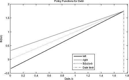
Stochastic DMPE with inelastic labor supply.
In an influential paper, Persson and Svensson (1989) argue that when governments are subject to a positive probability of being replaced, they set debt policy strategically. For instance, a right-leaning government issues more debt if it anticipates that it will be replaced by a left-leaning government with a stronger taste for public expenditure. In our model, the transition probabilities of the stochastic political process do not enter the equilibrium functions of Proposition 2. This implies that only the current political preferences matter in equilibrium. In contrast, the political equilibrium is not affected by the persistence of the political color of governments; in particular, a permanent political shift has the same effect as a temporary one. This surprising result hinges on the cancellation of an income and a substitution effect. Suppose, for example, that an incumbent left-leaning government anticipates a shift to the right. On the one hand, fiscal discipline today yields a lower return to left-wing voters since in the next period a right-leaning government will spend only a small share of potential resources, |$(\bar b - b^{\prime})$|, on public goods, and use instead a large part of them to cut taxes. This substitution effect reduces the incumbent left-leaning government’s wariness to debt accumulation. On the other hand, left-wing voters have a higher marginal utility of future government expenditure precisely when the next government has a lower propensity to spend on public goods. This income effect strengthens the fiscal discipline of the incumbent left-leaning government. Under logarithmic preferences and nondistortionary taxation, the income and substitution effects cancel out. In the general case, the sign of this strategic effect is ambiguous. However, as we will show in the next section, the size of the strategic effect is quantitatively very small in a calibrated economy featuring an empirically plausible labor supply elasticity.
In summary, in our environment the sign of the strategic effect emphasized by Persson and Svensson (1989) is ambiguous, being exactly zero under logarithmic preferences, and nondistortionary taxation. This ambiguity may explain why the empirical literature has found mixed support for this prediction (see Lambertini 2003; Pettersson-Lidbom 2001).
3.2. Elastic Labor Supply
In the general case with an elastic labor supply, |$\xi \gt 0$|, the DMPE does not admit a closed-form solution. However, our numerical analysis shows that the results are qualitatively similar to those derived with an inelastic labor supply. The main difference is that the debt policy function yields an interior determined government debt level even for a perpetual sequence of the same realization of the stochastic political process. The intermediate range of debt levels between the long-run debt level of the left and that of the right is the support of an ergodic debt distribution.10 Within such a range, the debt dynamics have the same qualitative features as those in Section 3.1: right-leaning governments accumulate debt while left-leaning governments reduce it. This is the main theoretical prediction that we will test in Section 5.
For the numerical analysis, we use a standard projection method with Chebyshev collocation to approximate the functions |$B(b,\theta ),G(b,\theta )$|, and |$T(b,\theta )$| characterized in Proposition 1.11 A summary of the values of all parameters is listed in Table 1.
Parameterization
| Target | Value | Parameter | Value |
|---|---|---|---|
| Capital’s income share of output | 1/3 | |$\alpha$| | 1/3 |
| World capital-output ratio (annualized) | 3.00 | |$R$| | (1.0410)30 |
| Domestic wage (normalization) | 1 | |$Q$| | 2.82 |
| Relative voter turnout for the old (61+) in the United States | 25% | |$\omega$| | 0.25 |
| World wealth-output ratio (annualized) | 3.539 | |$\beta$| | (0.986)30 |
| Effective tax rate | 17.2% | |$\lambda$| | 2.17 |
| Labor income tax rate at the top of the Laffer curve | 60% | |$\xi$| | 2/3 |
| Symmetric re-election probability four-year term | 50% | |$\rho$| | 0.5 |
| Debt–output ratio perpetual Democratic US Government | 29.7% | |$\theta _l$| | 0.563 |
| Debt–output ratio perpetual Republican US Government | 78.2% | |$\theta _r$| | 0.536 |
The length of a period is 30 years. The Frisch elasticity of labor supply is set to |$\xi = 2/3$|, which implies that the top of the Laffer curve is at |$\bar \tau = 60\% $|, in line with Trabandt and Uhlig (2011). We set |$\omega = 0.25$| to reflect the political influence of the old.12 We set |$\lambda = 2.17$| so as to match the federal tax revenue of 17.2% as a share of GDP in the United States over the period 1950–2013.13 This value of |$\lambda$| implies that the old care more for public goods than the young, a feature that we view as plausible (e.g., elderly people care about parks, street safety, etc.).
Regression for the United States, 1950–2013: debt accumulation
| Dep. variable | Debt growth, |$\Delta b_t \equiv b_{t + 1} - b_t$| | |||||
|---|---|---|---|---|---|---|
| (1) | (2) | (3) | (4) | (5) | (6) | |
| |${\text{demo}}_t$| | −2.531*** (−3.03) | −2.429*** (−4.06) | −2.357*** (−4.64) | −2.235*** (−4.86) | −1.992*** (−5.06) | −1.991*** (−5.00) |
| |$b_t$| | 0.016 (0.25) | −0.022 (−0.68) | −0.021 (−0.67) | −0.029 (−1.02) | −0.041* (−1.78) | −0.041* (−1.86) |
| |$u_{t - 1}$| | 0.447 (1.70) | 0.227 (0.95) | 0.309 (1.31) | 0.308 (1.38) | ||
| |$u_{t - 1} \times {\text{demo}}_{\text{t}}$| | 0.441 (1.72) | 0.180 (0.90) | 0.182 (0.86) | |||
| |${\text{Rec}}_t$| | 7.956*** (4.29) | 7.959*** (4.24) | ||||
| |${\text{elec}}_{\text{t}}$| | 0.015 (0.04) | |||||
| Controls | No | Yes | Yes | Yes | Yes | Yes |
| Observations | 63 | 63 | 63 | 63 | 63 | 63 |
| Adj. |$R^2$| | 0.077 | 0.498 | 0.520 | 0.519 | 0.711 | 0.706 |
Notes: |$b_t$| is the gross federal debt–output ratio at the beginning of fiscal year |$t$| reported in the historical tables of the Office of Management and Budget. |$\Delta b_t \equiv b_{t - 1} - b_t$| denotes debt growth in fiscal year |$t$|. |${\text{demo}}_t$| is a dummy variable which equals one or zero when the President of the United States is a Democrat or a Republican at the beginning of fiscal year |$t$|, respectively. |$u_t$| is the average unemployment rate in year |$t$| (demeaned), |${\text{Rec}}_t$| indicates fiscal years affected by the Great Recession, and |${\text{elec}}_t$| federal elections in fiscal year |$t$|. Control variables are the fraction of population aged above 65 and below 15, and US involvement in a major war. Standard errors are adjusted for clusters in the presidential term, and the robust |$t$|-statistics are reported in parentheses.
Significant at 1%
significant at 10%.
As a benchmark we assume the stochastic political process to be i.i.d.—that is, |$\pi (\theta ^{\prime} = \theta _s |\theta = \theta _s ) = 1/2$|, where |$\pi (\theta ^{\prime}|\theta )$| denotes the transition probabilities of the Markov process.17 The results are not sensitive to changes in the persistence parameters.
The annualized interest rate is set to |$R^{1/30} = 1.04$|. With a capital share of output of |$\alpha = 1/3$|, this implies an annualized capital-output ratio of 3. Finally, we set the parameter |$\beta$| to |$(0.986)^{30}$| so that the annualized ratio of net wealth to GDP of the economy is 3 at the average realization of |$\theta$|, where net wealth is defined as savings of the young minus government debt.
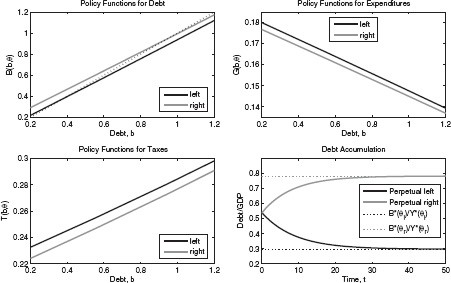
Figure 2 plots the policy function obtained from the numerical analysis for the case of i.i.d. political shocks. As in the analytical solution under inelastic labor supply, a political shift to the right shifts the debt policy upwards, |$B(b,\theta _l ) \lt B(b,\theta _r )$|, and both the tax and the government expenditure policy downwards, |$T(b,\theta _l ) \gt T(b,\theta _r )$| and |$G(b,\theta _l ) \gt G(b,\theta _r )$|. The bottom-right panel shows the pattern of debt accumulation in an economy with perpetual left- or right-leaning governments, respectively, starting from the average debt level in the stationary equilibrium. The long-run debt levels associated with perpetual rule of each party are pinned down by the intersection of the debt policy function |$B(b,\theta )$| with the 45–degree line in the top-left panel. If we denote these debt levels by |$B^* (\theta _r )$| and |$B^* (\theta _l )$|, respectively, the bottom-right panel shows the corresponding stationary debt–output levels, |$\tilde b^* (\theta _r ) \equiv B^* (\theta _r )/Y^* (\theta _r )$| and |$\tilde b^* (\theta _l ) \equiv B^* (\theta _l )/Y^* (\theta _l )$| As explained previously, our calibration implies |$\tilde b^* (\theta _r ) = 78.2\%$|, and |$\tilde b^* (\theta _l ) = 29.7\% $| respectively.
Stochastic DMPE with elastic labor supply.
Figure 3 shows the impulse-response of fiscal policy to a long sequence of right-leaning governments, starting from the long-run debt level |$\tilde b^* (\theta _l )$|. The figure shows different cases corresponding to alternative persistence parameters. If we denote by |$\rho$| the probability that the government at |$t + 1$| has the same color as the government at |$t$|, then, |$\rho = 1/2$| yields the benchmark i.i.d. case. This case is represented by the solid line. The dashed and the dash-dotted lines correspond to the case of high autocorrelation, |$\rho = 9/10$|, and negative autocorrelation, |$\rho = 1/10$| (assumed to be the same for both right- and left-leaning governments), respectively. The remaining parameters are unchanged. In spite of the large difference in persistence, the dashed and the dash-dotted lines are fairly close to the solid line representing the i.i.d. case. Thus, changes in the persistence of the political regime have small quantitative effects on debt accumulation. This reflects the fact that the size of the substitution effect is roughly equal to the opposing income effect for reasonable labor supply elasticities. The effect of strategic debt issuing is generally small.
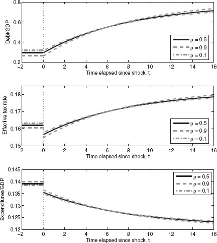
Policy response political shift to the right.
So far, we have assumed logarithmic utility. For robustness, in Figures D.2 and D.3 of the Online Appendix we display the numerical solution of our model when voters have preferences featuring a constant relative risk aversion |$(RRA)$| of two over both private and public good consumption. The results are similar to the logarithmic case.
3.3. Countercyclical Fiscal Policy
In this section, we outline an extension aimed to tease out the predictions of the theory about the cyclical properties of the fiscal policy. A complete model of business cycle fluctuations is beyond the scope of this paper. Instead, we consider a simple experiment in which we assume that the economy has fallen into a one-period recession. The downturn is expected to end in the following period and never to occur again. We start by considering the case of inelastic labor supply for which we can obtain an analytical solution.
The calibrated economy with elastic labor supply exhibits the same pattern as the economy with inelastic labor supply analyzed previously: in response to a one-time recession, all governments increase debt and reduce expenditure and tax revenue. We choose a recession that corresponds to a 10% drop in the young’s earnings at the average stationary debt level, and plot the changes of debt growth, expenditure, tax revenue, and consumption of the young in absolute levels (Figure D.4 in the Online Appendix) and as a fraction of GDP (Figure D.5 in the Online Appendix). The dotted vertical line in each panel indicates the average stationary debt level or debt–GDP ratio, respectively.
Left-leaning governments run larger deficits and increase the debt more than do right-leaning governments—see the top-left panel of Figure D.4. The same figure shows that both government expenditures and tax revenues fall in a recession, the absolute decline being larger for left- than for right-leaning governments. One should bear in mind, however, that GDP also falls in a recession. For the empirical predictions to be comparable with the empirical analysis in Section 5, we normalize the debt, expenditure, and tax revenue by the GDP level both in the data and in theory. Figure D.5 shows that the debt–GDP ratio increases for all debt levels compared to normal times, and more so for left-leaning governments. Thus, a robust prediction of the theory is that left-leaning governments pursue a more aggressive deficit-spending policy in recession—both in absolute levels, and normalized by GDP. Furthermore, Figure D.5 also illustrates that the expenditure–GDP ratio (top-right panel) is increasing and the effective tax rate falling (bottom-left panel) in response to the recession. The theory predicts that the expenditure–GDP ratio increases more under left-leaning governments, while right-leaning governments implement larger tax cuts. It is reassuring that the predictions of the calibrated economy are qualitatively in line with the (analytical) predictions of the inelastic labor supply economy laid out previously.
4. General Equilibrium
So far, we have taken the interest rate |$R$| as given. In this section, we determine the interest rate endogenously, assuming that there is a global capital market and that the world comprises a large number of countries with the same preferences, technology, and political process. The goal of this section is to derive predictions about the long-run distribution of debt across countries.
We focus first on the case with inelastic labor supply. In this case, we can characterize analytically the stationary equilibrium of the world economy. Later we extend the analysis to the case of elastic labor supply.
4.1. Stationary Political Equilibrium
Every period, each small open economy draws an idiosyncratic realization of the parameter |$\theta \in \{ \theta _l ,\theta _r \} $|. Consequently, even if the countries are ex-ante identical, a country’s debt depends on its individual history of shocks.
The state vector comprises the distribution of government debt and private wealth across countries. We focus on equilibria where the world interest rate is constant over time, and the policy rules of each country are functions of the country-specific state variables (as analyzed previously) and the constant world interest rate |$R$|. In doing so, we follow the equilibrium concept pioneered in Huggett (1993) and Aiyagari (1994). We focus on a slightly more general stationary equilibrium definition than in Huggett (1993) and Aiyagari (1994)—a quasi-stationary equilibrium—that allows the cross-country debt distributions to be expanding over time, although the mean debt level conditional on the realized shock, |$\theta$|, is constant over time. Since we allow for ever-expanding distributions, we also impose no lower bounds on government debt and taxes, |$b^{\prime} \in ( - \infty ,\bar b(R) \equiv \bar \tau H(\bar \tau )/(R - 1)]$| and |$\tau \in ( - \infty ,1]$|.19
Let |$\{ \chi _t \} _{t = 0}^\infty$| be a set of probability measures defined on |$(\Omega ,\Sigma _\Omega )$|, where |$\Omega = ( - \infty ,b(R)] \times \{ \theta _l ,\theta _r \}$| is the individual state space, and |$\Sigma _\Omega$| is the Borel |$\sigma$|-algebra on |$\Omega$| (i.e., the set of all possible subsets of |$\Omega$|). Thus, for any set |$x \in \Sigma _\Omega $|, the measure of countries whose individual state vectors lie in the set |$x$| in period |$t$| is given by |$\chi _t (x)$|.
Definition 2
A quasi-stationary Markov-perfect political equilibrium (QSMPE) is a constant interest rate|$R^*$|, a sequence of probability measures|$\{ \chi _t \} _{t = 0}^\infty$| defined on |$(\Omega ,\Sigma _\Omega )$|, and a set of functions|$\left\langle {B,G,T} \right\rangle $|, where|$B:\Omega \times {\Bbb R}^ + \to ( - \infty ,\bar b(R)]$|is a debt rule, |$b^{\prime} = B(b,\theta ,R),G:\Omega \times {\Bbb R}^ + \to [0,\infty )$|, is a government expenditure rule, |$g = G(b,\theta ,R)$|, and |$T:\Omega \times {\Bbb R}^ + \to ( - \infty ,1]$|is a tax rule, |$\tau = T(b,\theta ,R)$|, such that the domestic political equilibrium conditions in (11)(12) and (13) of Proposition2 are satisfied for|$b^{\prime} \in ( - \infty ,\bar b(R^* )]$|and, in addition, the following three conditions hold.
In the following, we provide a proposition that illustrates the functional form of the quasi-stationary equilibrium interest rate when the political shock has no persistence.20
Proposition 3
Note that Corollary 1 applies to this stationary equilibrium interest rate. Therefore, the discussion of the political equilibrium under political shocks provided in Section 3.1, including the location of the debt policy rules in Figure 1, apply even when the world economy is restricted to be in a stationary equilibrium: right-leaning governments accumulate debt, while left-leaning governments reduce the debt level.
A similar result applies to the calibrated economy with elastic labor supply that we analyzed in Section 3.2. First, note that the equilibrium Definition 2 applies also to the case of elastic labor supply. For all parameter configurations we have tried, we have found a unique equilibrium consistent with Definition 2—that is, a QSMPE.21 However, with an elastic labor supply the equilibrium we have found features a unique time-invariant stationary distribution in the long run. More precisely, there exists a measure |$\chi ^*$| defined on |$(\Omega ,\Sigma _\Omega )$| such that |$\chi ^* = \chi _t$| for all |$t \ge 0$|, and the cross-country distribution of debt converges to |$\chi ^*$| regardless of the initial distribution of debt.
Second, recall that |$\beta$| was calibrated so that when simulating the economy for a very long time and taking the sample average for the economy, the annualized average domestic private wealth to GDP ratio minus the annualized domestic government debt to GDP ratio was equal to 3. Such a level of capital would, in a closed economy, generate an annualized return to capital of |$R^{1/30} = 1.04$|. Moreover, note that when the stationary equilibrium is unique, the moments of a sufficiently long realization of an individual economy do converge to the stationary equilibrium distribution regardless of the initial conditions (see Aiyagari 1994). This implies that the calibrated economy of Section 3.2 actually coincides with the allocations in a general stationary equilibrium consistent with Definition 2.22
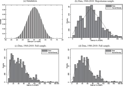
Note that in equilibrium, the range of the stationary distribution of cross-country debt equals |$(B^* (\theta _l ;R^* ),B^* (\theta _r ;R^* ))$|, where the notation |$B^* (\theta ;R^* )$| denotes the debt level an individual economy will converge to, given an interest rate |$R^*$| and an arbitrarily long sequence of realizations |$\theta _t = \theta$|. Hence, in the long run the debt of every country is bounded between the limiting debt levels |$B^* (\theta _r ;R^* )$| and |$B^* (\theta _l ;R^* )$|. We plot the stationary debt distribution consistent with our parameterization in the top-left panel of Figure 4. By targeting the bounds of the ergodic set alone, our model generates a unimodal distribution of government debt across countries, which is broadly in line with the empirical distribution that we observe for the United States and other OECD countries with a majoritarian electoral system over the period 1960–2010 (top-right panel).23 Given that political shocks are the only source of variation in the model, it seems reasonable that the empirical debt distribution appears more spread out as it is affected by other shocks as well. The two bottom panels show the empirical distribution for the full panel of 24 OECD countries that we consider for the empirical analysis in Section 5.2. In that sample the debt–GDP ratios are more skewed to the right than the benchmark parameterization of our model predicts. The mass point around 110% of GDP is mostly driven by Greece, Italy, and Belgium, and the observations in the upper tail are those of Japan. Those debt levels might be the result of shocks that are not part of our theory.
Stationary debt distribution.
Recall that our hypothesis that right-leaning governments accumulate debt while left-leaning governments reduce it applies only to countries with a debt level in between |$B^* (\theta _l ;R^* )$| and |$B^* (\theta _r ;R^* )$|. This coincides with the support of the stationary distribution, which in turn implies that in the absence of other shocks than those to |$\theta$|, our theoretical hypothesis will be the empirically relevant prediction in the long run. To see this, consider a country that starts with a debt level above the maximum stationary debt level |$B^* (\theta _r ;R^* )$|. Such a situation might have occurred due to a shock we have not modeled here, for example a large one-time exogenous government spending requirement due to, say, a natural disaster or a war. In the aftermath of the disaster, such a country will reduce the initial high debt no matter what is the political color of its government.24 However, once the debt is back in the stationary range, it will again follow the dynamics of Proposition 2.
Finally, note that if a shock to debt for some reason were to move debt out of the stationary region, debt will eventually revert to the stationary region. Moreover, recall that any stationary stochastic process exhibits some mean reversion. It follows that the dynamics of debt in this model imply some mean reversion of debt.
5. Empirical Evidence
In this section, we test the empirical predictions of the theory. Our model predicts that debt accumulation should be larger under right-leaning than under left-leaning governments. It also predicts—under the realistic assumption of distortionary taxation—that debt is mean reverting. For this reason, we follow the empirical specification of Bohn (1998), who regresses debt growth in the United States on the initial debt–GDP ratio, and introduce dummies capturing the political inclination of governments. Since the low-frequency dynamics of government debt is driven by demographic variables determining the financing needs of the pension system and health expenditure, we control in our regressions for the fraction of population aged above 65 and below 15. We also control for unemployment to filter out the cyclical component of the debt–GDP ratio, due to both automatic factors (such as the reduction of the tax revenue during recessions) and active fiscal policy at business cycle frequencies. This also allows us to test the prediction that left-leaning governments adopt more countercyclical debt policies.
We consider first the time-series analysis for the United States. The United States is a natural testing ground, since it has a presidential two-party system where, at least since World War II, the Republican Party has positioned itself consistently to the right of the Democratic Party.25 Then, we extend the analysis to the effects of political shifts within countries in a panel of OECD countries. This extension poses some challenges. In many continental European countries, the classification of the color of governments is ambiguous, due to the frequent occurrence of coalition governments, resulting in significant measurement error.26 With this motivation, we present first the results for the full sample of countries for which data are available, and then restrict the sample to countries with a majoritarian electoral system. Following the classification of Persson and Tabellini (1999), this sample comprises Australia, Canada, France, the United Kingdom, and the United States. In all these countries, the data show a clear-cut alternation in power between left- and right-leaning governments.
A caveat is that we treat political shifts as exogenous, ignoring feedbacks from the debt policy to the probability that the incumbent party is re-elected. While such feedbacks cannot be ruled out, they are unlikely to have a major effect on our estimated coefficients. Given the difficulty in finding valid instruments, we do not try to address this possible endogeneity issue, and interpret the results as correlations.
5.1. United States
The data for US fiscal policy are from the historical tables of the US Office of Management and Budget. The civilian unemployment rate is from the Bureau of Labor Statistics, and the demographic variables are from the OECD (2014) Employment and Labour Market Statistics database.
Table 2 reports the estimation results, with cluster-robust |$t$|-statistics in parentheses. Standard errors are adjusted for cluster correlation within presidential terms (alternative clustering strategies are discussed in what follows in the robustness section). The estimate of our main coefficient of interest, |$\beta _1$|, yields an average effect of a democratic administration over the presidential term which allows for potentially sluggish effects of the color of the administration on fiscal policy.
A Democratic presidency is associated with an average reduction in the debt–GDP ratio ranging between an annual 2% and 2.5% across the different specifications. The estimated coefficients are statistically significant at the 1% level. Column (1) reports the result of a specification without further control variables. Controlling for war and demographic structure reduces only marginally the absolute value of the estimate of |$\beta _t$| (column (2)). The results are robust to filtering out changes in the debt–GDP ratio associated with business cycle fluctuations, proxied by the lagged unemployment rate (column (3)). The coefficient on the lagged debt–GDP ratio is negative, consisting with Bohn’s result that debt is mean reverting, being significant at the 10% level in the specifications of columns (5) and (6) including all controls.
Column (4) shows the interesting result that Democratic administrations adopt more countercyclical debt policies than do Republican administrations—although the effect is marginally insignificant. This is consistent with the extension outlined in Section 3.3 predicting that left-leaning governments should be more prone to issue debt during recessions. While this result is more fragile, the main effect of the administration’s color is robust: Democratic administrations are less prone to debt accumulation when the unemployment rate is at its average level. Finally, in columns (5) and (6), we introduce a dummy switching on during the Great Recession (2008–2010). The Great Recession has a large and highly significant positive effect on debt accumulation. The estimated coefficient of |${\text{demo}}_t$| falls slightly in absolute value, but remains highly significant. In other words, the Obama administration appears to follow the tradition of Democratic administrations to respond to recessions by robust increases in the debt–GDP ratio. Its response is in fact stronger than usual, likely due to the particular features of the crisis and of the policy response.
Our theory also predicts that, conditional on the debt level, Democratic administrations tax and spend more. To test this further prediction, we repeat the time-series regression specified in equation (14) with taxes and nondefense expenditures as the dependent fiscal variables. Taxation is measured by US federal tax revenue as a fraction of GDP. Table 3 shows that, conditional on the outstanding debt–GDP ratio, Democratic administrations raise more taxes. The estimated effects are stable across specifications and statistically significant. The magnitude of the coefficient is around 0.7 percentage points. The negative and statistically significant coefficient of |$u_{t - 1}$| confirms that Republican administrations offer tax cuts during recessions as do Democratic administrations. The interaction effect is insignificant (with a negative point estimate that would go against the prediction of the theory). All the results are robust to the inclusion of a dummy for the Great Recession.
Regression for the United States, 1950–2013: effective tax rate.
| Dep. variable | Effective tax rate, |$\tau _t$| | |||||
|---|---|---|---|---|---|---|
| (1) | (2) | (3) | (4) | (5) | (6) | |
| |${\text{demo}}_t$| | 0.775* (1.95) | 0.834** (2.44) | 0.762*** (3.07) | 0.726*** (3.09) | 0.689*** (2.93) | 0.687** (2.85) |
| |$b_t$| | −0.030** (−2.15) | −0.026** (−2.47) | −0.028*** (−3.73) | −0.025*** (−3.44) | −0.024*** (−3.48) | −0.023*** (−3.42) |
| |$u_{t - 1}$| | −0.447*** (−6.38) | −0.382*** (−5.60) | −0.394*** (−5.61) | −0.389*** (−5.63) | ||
| |$u_{t - 1} \times {\text{demo}}_t$| | −0.131 (−1.22) | −0.092 (−0.88) | −0.100 (−0.89) | |||
| |${\text{Rec}}_t$| | −1.196** (−2.57) | −1.214** (−2.62) | ||||
| |${\text{elec}}_t$| | −0.081 (−0.61) | |||||
| Controls | No | Yes | Yes | Yes | Yes | Yes |
| Observations | 63 | 63 | 63 | 63 | 63 | 63 |
| Adj. |$R^2$| | 0.214 | 0.269 | 0.617 | 0.619 | 0.664 | 0.659 |
Notes: |$\tau _t$| is total federal tax revenue as a fraction of output in fiscal year |$t$|, and |$b_t$| is the gross federal debt–output ratio at the beginning of fiscal year |$t$| reported in the historical tables of the Office of Management and Budget. |${\text{demo}}_t$| is a dummy variable which equals one or zero when the President of the United States is a Democrat or a Republican at the beginning of fiscal year |$t$|, respectively. |$u_t$| is the average unemployment rate in year |$t$| (demeaned), |${\text{Rec}}_t$| indicates fiscal years affected by the Great Recession, and |${\text{elec}}_t$| federal elections in fiscal year |$t$|. Control variables are the fraction of population aged above 65 and below 15, and US involvement in a major war. Standard errors are adjusted for clusters in the presidential term, and the robust |$t$|-statistics are reported in parentheses.
Significant at 1%
significant at 5%
significant at 10%.
Next, we consider federal nondefense government expenditure as percentage of GDP. Although defense is a public good, it is fundamentally different from other goods, being largely driven by international conflicts. Clearly, our assumption that left-wing voters value public good provision more than do right-wing voters cannot capture military expenditure. Table 4 reports the results. Conditional on debt, we find a robust positive effect of the Democratic administration dummy. These spend ca. 0.6 percentage points more on federal nondefense expenditures compared to Republican administrations. The expenditure–GDP ratio increases in recession under any administration, and more so under Democratic administrations. These results conform with the predictions of the theory, and are again robust to the inclusion of a dummy for the Great Recession.
Regression for the United States, 1950–2013: nondefense expenditures.
| Dep. variable | Nondefense expenditures, |$g_t$| | |||||
|---|---|---|---|---|---|---|
| (1) | (2) | (3) | (4) | (5) | (6) | |
| |${\text{demo}}_t$| | −0.108 (−0.07) | 0.406 (1.73) | 0.483*** (2.92) | 0.535*** (2.92) | 0.582*** (3.38) | 0.586*** (3.49) |
| |$b_t$| | −0.013 (−0.21) | −0.065*** (−4.85) | −0.063*** (−9.58) | −0.067*** (−11.01) | −0.069*** (−11.97) | −0.070*** (−12.31) |
| |$u_{t - 1}$| | 0.473*** (6.13) | 0.380*** (3.84) | 0.395*** (3.85) | 0.385*** (3.81) | ||
| |$u_{t - 1} \times {\text{demo}}_t$| | 0.188* (1.85) | 0.138 (1.31) | 0.154 (1.53) | |||
| |${\text{Rec}}_t$| | 1.529** (2.43) | 1.565** (2.51) | ||||
| |${\text{elec}}_t$| | 0.161 (1.08) | |||||
| Controls | No | Yes | Yes | Yes | Yes | Yes |
| Observations | 63 | 63 | 63 | 63 | 63 | 63 |
| Adj. |$R^2$| | −0.029 | 0.928 | 0.960 | 0.961 | 0.967 | 0.967 |
Notes: |$g_t$| is nondefense expenditures as fraction of output in fiscal year |$t$| and |$b_t$| is the gross federal debt–output ratio at the beginning of fiscal year |$t$| reported in the historical tables of the Office of Management and Budget. |${\text{demo}}_t$| is a dummy variable which equals one or zero when the President of the United States is a Democrat or a Republican at the beginning of fiscal year |$t$|, respectively. |$u_t$| is the average unemployment rate in year |$t$| (demeaned), |${\text{Rec}}_t$| indicates fiscal years affected by the Great Recession, and |${\text{elec}}_t$| federal elections in fiscal year |$t$|. Control variables are the fraction of population aged above 65 and below 15, and US involvement in a major war. Standard errors are adjusted for clusters in the presidential term, and the robust |$t$|-statistics are reported in parentheses.
Significant at 1%
significant at 5%
significant at 10%.
5.1.1. Robustness
In this section we consider various robustness tests of our previous empirical results.
Parties’ Control over Congress
In Tables 2–4 we focus on the party affiliation of the sitting US President. However, it is not uncommon for the party of the president not to hold the majority of seats in one or both chambers of the US Congress. This can in principle affect the conduct of fiscal policy. In Table 5, we report the results of regressions where we break down the effect of the color of the administration by the extent to which they control the US Senate or the House of Representatives.
Regression for the United States, 1950–2013: minority in the US Congress
| Dep. variable | Debt growth, |$\Delta b_t$| | Effective tax rate, |$\tau _t$| | Nondefense exp., |$g_t$| | ||||||
|---|---|---|---|---|---|---|---|---|---|
| (1) | (2) | (3) | (4) | (5) | (6) | (7) | (8) | (9) | |
| |${\text{demo}}_t$| | −2.784*** (−3.71) | −2.857*** (−3.60) | −2.295*** (−4.23) | 0.747** (2.66) | 0.765** (2.80) | 0.682** (2.32) | 0.936*** (3.62) | 0.911*** (3.52) | 1.039*** (6.26) |
| |${\text{minor}}_t$| | −1.689** (−2.29) | −1.852** (−2.38) | −1.218* (−1.88) | 0.245 (0.93) | 0.285 (1.11) | 0.191 (0.70) | 0.705*** (3.05) | 0.650** (2.83) | 0.794** (4.67) |
| |${\text{minor}}_t \times {\text{demo}}_t$| | −0.929 (−0.84) | −0.356 (−0.29) | −0.863 (−0.80) | 0.498 (1.16) | 0.356 (0.81) | 0.431 (0.95) | −0.914* (−1.91) | −0.721 (−1.60) | −0.836** (−2.19) |
| |$b_t$| | −0.023 (−0.82) | −0.030 (−1.28) | −0.040* (−2.02) | −0.028*** (−3.76) | −0.026*** (−3.52) | −0.024*** (−3.61) | −0.062*** (−12.24) | −0.065*** (−12.86) | −0.067*** (−16.08) |
| |$u_{t - 1}$| | 0.209 (0.74) | 0.053 (0.22) | 0.160 (0.61) | −0.379*** (−4.67) | −0.340*** (−4.73) | −0.356*** (−4.86) | 0.453*** (7.24) | 0.400*** (5.40) | 0.424*** (5.80) |
| |$u_{t - 1} \times {\text{demo}}_t$| | 0.389 (1.45) | 0.103 (0.56) | −0.096 (−0.98) | −0.054 (−0.55) | 0.131 (1.52) | 0.067 (0.70) | |||
| |${\text{Rec}}_t$| | 7.580*** (4.07) | −1.125** (−2.29) | 1.718** (2.84) | ||||||
| Controls | Yes | Yes | Yes | Yes | Yes | Yes | Yes | Yes | Yes |
| Observations | 63 | 63 | 63 | 63 | 63 | 63 | 63 | 63 | 63 |
| Adj. |$R^2$| | 0.559 | 0.556 | 0.733 | 0.636 | 0.633 | 0.673 | 0.963 | 0.963 | 0.971 |
Notes: |$b_t$| is the gross federal debt–output ratio at the beginning of fiscal year |$t$|, |$\tau _t$| total tax revenue as a fraction of output, and |$g_t$| is nondefense expenditures as fraction of output in fiscal year |$t$|, as reported in the historical tables of the Office of Management and Budget. |$\Delta b_t \equiv b_{t + 1} - b_t$| denotes debt growth and |${\text{demo}}_t$| is a dummy variable which equals one or zero when the President of the United States is a Democrat or a Republican at the beginning of fiscal year |$t$|, respectively. |$u_t$| is the average unemployment rate in year |$t$| (demeaned), |${\text{minor}}_t$| indicates US Presidents without a majority in either chamber of the congress, and |${\text{Rec}}_t$| indicates fiscal years affected by the Great Recession. Control variables are the fraction of population aged above 65 and below 15, and US involvement in a major war. Standard errors are adjusted for clusters in the presidential term, and the robust |$t$|-statistics are reported in parentheses.
Significant at 1%
significant at 5%
significant at 10%.
The estimates of the political variables reported in Table 5 are relative to the benchmark of a “strong” Republican presidency in which the Republican Party holds the majority in at least one of the chambers of the US Congress. The coefficient of |${\text{demo}}_t$| yields the effect of a “strong” Democratic presidency relative to the benchmark. If the party of the President controls (at least in part) the US Congress, Democratic administrations accumulate less debt, and choose higher taxes and higher nondefense government expenditures relative to Republican administrations. Interestingly, the lack of control over the congress tends to reduce debt accumulation under both Republican and Democratic administrations. The effect of not controlling the congress is stronger for Republican presidencies, where it is highly significant, while it is smaller in absolute value and statistically insignificant for Democratic presidencies. In general, the evidence suggests that more fiscal discipline is forced upon the administration of both colors, although the effect is especially strong for Republican presidents. The regression for taxes (columns (4)–(6)) shows no significant effects of the party controlling the US Congress. Finally, lack of control over the congress appears to imply more nondefense expenditure under Republican administrations, and less nondefense expenditure under Democratic administrations (columns (7)–(9)), suggesting that a hostile congress imposes tighter constraints on the choice of the executive.
In summary, the results of Table 5 show that while the identity of the party holding a majority in the congress is sometimes significant, but overall fragile, its inclusion does not affect the main result of the previous section: Democratic administrations accumulate less debt, and choose higher taxes and higher nondefense government expenditures relative to Republican administrations.
We also test the robustness of the results to a finer classification of the political control over the congress and executive. In Table 6, we include in the regression an index for Democratic political control ranging from 1 (Republicans control presidency, House of Representatives and Senate) and 6 (Democrats control presidency, House of Representatives and Senate) instead of the |${\text{demo}}_t$| dummy.30 The results are largely robust. A higher value of the index is associated with less debt accumulation, higher taxes, and higher expenditure. Because of the categorical nature of the index, it is no longer possible to give the estimated coefficient a simple quantitative interpretation. However, the coefficients are estimated very precisely and are highly significant.
Regression for the United States, 1950–2013: index for Democratic political control
| Dep. variable | Debt growth, |$\Delta b_t$| | Effective tax rate, |$\tau _t$| | Nondefense exp., |$g_t$| | ||||||
|---|---|---|---|---|---|---|---|---|---|
| (1) | (2) | (3) | (4) | (5) | (6) | (7) | (8) | (9) | |
| |${\text{demo_Index}}_t$| | −0.563*** (−4.06) | −0.539*** (−4.15) | −0.532*** (−5.10) | 0.191** (2.83) | 0.185** (2.88) | 0.184** (2.70) | 0.189*** (5.28) | 0.198*** (5.20) | 0.200*** (5.87) |
| |$b_t$| | −0.031 (−1.05) | −0.040 (−1.55) | −0.049** (−2.36) | −0.025*** (−3.56) | −0.022*** (−3.47) | −0.021*** (−3.55) | −0.063*** (−11.10) | −0.066*** (−12.40) | −0.068*** (−12.88) |
| |$u_{t - 1}$| | 0.576* (1.93) | 0.044 (0.15) | 0.320 (1.08) | −0.490*** (−5.38) | −0.359*** (−3.02) | −0.403*** (−3.24) | 0.436*** (6.45) | 0.224** (2.16) | 0.272** (2.33) |
| |$u_{t - 1} \times {\text{demo_Index}}_t$| | 0.140* (2.09) | 0.052 (1.06) | −0.034 (−1.26) | −0.020 (−0.74) | 0.055** (2.68) | 0.040 (1.62) | |||
| |${\text{Rec}}_t$| | 8.295*** (4.65) | −1.323*** (−3.23) | 1.423** (2.16) | ||||||
| Controls | Yes | Yes | Yes | Yes | Yes | Yes | Yes | Yes | Yes |
| Observations | 63 | 63 | 63 | 63 | 63 | 63 | 63 | 63 | 63 |
| Adj. |$R^2$| | 0.490 | 0.492 | 0.701 | 0.590 | 0.590 | 0.647 | 0.964 | 0.965 | 0.970 |
Notes: |$b_t$| is the gross federal debt–output ratio at the beginning of fiscal year |$t$|, |$\tau _t$| total tax revenue as a fraction of output, and |$g_t$| is nondefense expenditures as fraction of output in fiscal year |$t$|, as reported in the historical tables of the Office of Management and Budget. |$\Delta b_t \equiv b_{t + 1} - b_t$| denotes debt growth and |${\text{demo_Index}}_t$| is an index for Democratic political power at the beginning of fiscal year |$t$|, ranging from 1 (Republicans control presidency, house, and senate) to 6 (Democrats control presidency, house, and senate). |$u_t$| is the average unemployment rate in year |$t$| (demeaned), and |${\text{Rec}}_t$| indicates fiscal years affected by the Great Recession. Control variables are the fraction of population aged above 65 and below 15, and US involvement in a major war. Standard errors are adjusted for clusters in the presidential term, and the robust |$t$|-statistics are reported in parentheses.
Significant at 1%
significant at 5%
significant at 10%.
Alternative Business Cycle Indicators
In our main specification we control for unemployment. This is a common proxy for business cycle fluctuations, and has the advantage of being available in a standardized format for the whole set of OECD countries that we consider in the panel regression that follows. It is also a highly visible indicator to politicians and voters. In this section, we show that the results are robust to three alternative proxies of the cyclical level of economic activity: Total Factor Productivity (TFP) growth, a recession dummy according to the NBER classification, and the change (rather than the level) of the unemployment rate.
Table 7 presents the regression results for debt growth, taxes, and nondefense expenditure when we control for the lagged TFP growth |$(\Delta {\text{TFP}}_{t - 1} )$|, based on the estimate of TFP growth provided by the Bureau of Labor Statistics’ Multifactor Productivity Database. In order to interpret the coefficients of the interaction model, we measure TFP growth as the deviation from the sample average. The regressions where debt growth is the dependent variable (columns (1)–(3)) yield similar results for the coefficient of interest as in the baseline model. The effect of |$\Delta {\text{TFP}}_{t - 1}$| is significant and has the expected sign: when TFP growth falls, there is more debt accumulation. The results for taxes (columns (4)–(6)) and government expenditures (columns (7)–(9)) are also in accordance with the predictions of the theory.
Regression for the United States, 1950–2013: controlling for TFP growth
| Dep. variable | Debt growth, |$\Delta b_t$| | Effective tax rate, |$\tau _t$| | Nondefense exp., |$g_t$| | ||||||
|---|---|---|---|---|---|---|---|---|---|
| (1) | (2) | (3) | (4) | (5) | (6) | (7) | (8) | (9) | |
| |${\text{demo}}_t$| | −2.186*** (−3.77) | −2.154*** (−3.56) | −1.942*** (−3.54) | 0.835** (2.44) | 0.844** (2.42) | 0.799** (2.29) | 0.451* (2.10) | 0.441* (1.97) | 0.489* (2.11) |
| |$b_t$| | −0.007 (−0.23) | −0.004 (−0.14) | −0.024 (−1.12) | −0.026** (−2.24) | −0.026* (−2.05) | −0.021* (−2.10) | −0.062*** (−4.43) | −0.063*** (−4.46) | −0.068*** (−5.68) |
| |$\Delta {\text{TEP}}_{t - 1}$| | −0.679** (−2.83) | −0.567** (−2.70) | −0.411*** (−3.74) | −0.001 (−0.02) | 0.030 (0.51) | −0.003 (−0.07) | −0.124 (−1.47) | −0.157 (−1.67) | −0.121 (−1.43) |
| |$\Delta {\text{TEP}}_{t - 1} \times {\text{demo}}_t$| | −0.388 (−1.05) | −0.275 (−0.71) | −0.106 (−0.94) | −0.130 (−1.20) | 0.115 (0.86) | 0.140 (1.00) | |||
| |${\text{Rec}}_t$| | 7.118*** (4.00) | −1.485** (−2.33) | 1.609* (1.88) | ||||||
| Controls | Yes | Yes | Yes | Yes | Yes | Yes | Yes | Yes | Yes |
| Observations | 63 | 63 | 63 | 63 | 63 | 63 | 63 | 63 | 63 |
| Adj. |$R^2$| | 0.595 | 0.595 | 0.742 | 0.256 | 0.249 | 0.313 | 0.930 | 0.930 | 0.936 |
Notes: |$b_t$| is the gross federal debt–output ratio at the beginning of fiscal year |$t$|, |$\tau _t$| total tax revenue as a fraction of output, and |$g_t$| is nondefense expenditures as fraction of output in fiscal year |$t$|, as reported in the historical tables of the Office of Management and Budget. |$\Delta b_t \equiv b_{t + 1} - b_t$| denotes debt growth, and |${\text{demo}}_t$| is a dummy variable which equals one or zero when the President of the United States is a Democrat or a Republican at the beginning of fiscal year |$t$|, respectively. |$\Delta {\text{TEP}}_t$| is the TFP growth in year |$t$| (demeaned) and |${\text{Rec}}_t$| indicates fiscal years affected by the Great Recession. Control variables are the fraction of population aged above 65 and below 15, and US involvement in a major war. Standard errors are adjusted for clusters in the presidential term, and the robust |$t$|-statistics are reported in parentheses.
Significant at 1%
significant at 5%
significant at 10%.
The results are also robust to using the lagged change in unemployment, |$\Delta u_{t - 2} \equiv u_{t - 1} - u_{t - 2} $|, or a dummy classifying as recessions fiscal years in which the NBER classifies at least six months as recession times. We report the detailed results in Tables D.1 and D.2 of the Online Appendix.
Miscellaneous
The standard errors reported in Tables 2–4 are adjusted for cluster correlation within presidential terms. Adjusting the error bands instead for autocorrelation among unclustered observations (following Newey and West 1987) yields less conservative confidence intervals and more significant coefficients. The results are reported in Tables D.3–D.5 of the Online Appendix. There, we also report the standard errors that result from clustering years with the same US President (Table D.6), or that are resampled from clusters in presidential terms (Tables D.7–D.9).31 All clustering strategies yield highly significant coefficients for the political variable of interest in all specifications.
In the empirical specification presented in equation (14) we run an autoregressive specification in the spirit of Bohn (1998). When debt growth is the dependent variable, |$1 - \beta _2$| can be interpreted as the autoregressive coefficient of the initial stock of debt, |$b_t $|. Coherent with the structure of our theoretical model, we use the same specification for the regressions with the average tax rate and government expenditures as the dependent variables. The results are robust if we control for |$b_{t - 1}$| instead of |$b_t$| to caution against potential endogeneity concerns. As reported in Tables D.10–D.12 of the Online Appendix, the coefficient of the political variable remains overall highly significant across most specifications. The size of the coefficient is also similar. Furthermore, in Table D.13 we show that our results hold up independently of whether the US federal debt is measured gross or net of debt held by other federal government accounts, and in Table D.14 that our results are robust to including the cyclical component of defense expenditures as an additional control variable. In the latter specification, we separate the cyclical from the trend component of defense expenditures using a Hodrick–Prescott filter with smoothing parameter 100.
A final robustness test concerns the demographic control variables. As discussed in our previous work (SSZ), we believe that there is a structural link between demographic trends and debt dynamics. However, one might be concerned that the correlation between these two variables be spurious and simply driven by a common trend. To address this concern, we replace the demographic variable by its (lagged) first difference. The results for the regressions in which debt growth and the average tax rate are the dependent variables are unchanged (see Tables D.15 and D.16). However, the coefficient of the political variable for nondefense government expenditures turns insignificant and switches sign (Table D.17).
5.2. Panel of OECD Economies
In this section, we consider a panel of 24 OECD economies for the period 1950–2010, using the data on debt–GDP ratios collected by Reinhart and Rogoff (2011).32 We control for time-invariant heterogeneity and for common trends by including country fixed effects and time dummies. We classify the political inclination of governments following Woldendorp,Keman, and Budge (2000, 2011) who assign scores for government and parliament ranging from left-wing dominance to right-wing dominance.33 Since coalition governments introduce a severe measurement error, we also present the results for a subsample of five countries in which the electoral rule follows a majoritarian principle. In all such countries, there is an unambiguous alternation of governments between “left” and “right”. When we analyze the majoritarian subsample, we eliminate the dummy “center” and stick to a binary left–right classification.34
The results with the full sample are reported in Table 8. The coefficient for the left-leaning government dummy is consistently negative across all specifications. However, the coefficient is statistically significant for the period 1950–2007, but turns insignificant when the Great Recession is included. In columns (5) and (6), we include the entire sample period, and allow for the debt policy of right- and left-leaning governments to respond differently to business cycle fluctuations, in particular to the Great Recession. The results indicate heterogeneity in the response to the Great Recession: left-leaning governments expand debt on average 2.7% more annually than do right-leaning governments. This heterogeneity conforms with the prediction of the extension in Section 3.3. In normal times, a political switch to the left is associated with an average reduction in debt accumulation of 0.54% (column (6)), about a third of the effect estimated in the time-series analysis for the US. The coefficient is significant at the 10% level. There are no significant differences between center and right-leaning. The high debt accumulation of center governments is likely to be due to the bargaining process between coalition partners. Finally, the debt level is significantly mean reverting.
Panel regression for the OECD, 1950–2010: debt accumulation
| Dep. variable | Debt growth, |$\Delta b_t \equiv b_{t + 1} - b_t$| | ||||||
|---|---|---|---|---|---|---|---|
| Sample | 1950–2010 | 1950–2007 | 1950–2010 | ||||
| (1) | (2) | (3) | (4) | (5) | (6) | ||
| |${\text{left}}_t$| | −0.117 (−0.42) | −0.194 (−0.68) | −0.277 (−0.94) | −0.640** (−2.11) | −0.484 (−1.60) | −0.539* (−1.83) | |
| |${\text{center}}_t$| | 0.001 (0.00) | 0.137 (0.36) | 0.097 (0.25) | −0.194 (−0.49) | −0.085 (−0.22) | −0.092 (−0.24) | |
| |$b_t$| | −0.028*** (−3.59) | −0.036*** (−3.47) | −0.038*** (−3.34) | −0.042*** (−3.71) | −0.038*** (−3.34) | −0.038*** (−3.31) | |
| |$u_{t - 1}$| | 0.208*** (3.50) | 0.238*** (3.91) | 0.209*** (3.53) | 0.187** (2.36) | |||
| |$u_{t - 1} \times {\text{left}}_t$| | 0.084 (0.91) | ||||||
| |$u_{t - 1} \times {\text{center}}_t$| | −0.028 (−0.28) | ||||||
| |${\text{Rec}}_t$| | 3.668*** (2.76) | 3.635*** (2.75) | |||||
| |${\text{Rec}}_t \times {\text{left}}_t$| | 2.712** (2.06) | 2.716** (2.06) | |||||
| |${\text{Rec}}_t \times {\text{center}}_t$| | 3.230 (1.16) | 3.183 (1.14) | |||||
| Controls | No | Yes | Yes | Yes | Yes | Yes | |
| Observations | 1288 | 1193 | 1160 | 1096 | 1160 | 1160 | |
| Adj. |$R^2$| | 0.306 | 0.325 | 0.306 | 0.271 | 0.309 | 0.309 | |
Notes: Country and year dummies are included to control for country and time fixed-effects. |$b_t$| is the year |$t$| debt–output ratio reported in Reinhart and Rogoff (2011). |${\text{left}}_t$| stands for a left-leaning and |${\text{center}}_t$| for a center or coalition government in office at the end of year |$t$|. |$u_t$| is the average unemployment rate (demeaned), and |${\text{Rec}}_t$| indicates fiscal years affected by the Great Recession. Control variables are the fraction of population aged over 65 and below 15. Robust |$t$|-statistics are reported in parentheses.
Significant at 1%
significant at 5%
significant at 10%.
The results are stronger, and more precisely estimated, in the subsample of countries with a majoritarian electoral system—see Table 9. In this case, a political shift to the left implies on average a reduction in debt accumulation between 0.61% and 0.71% (columns (3)–(6)), statistically significant at the 1% level.
Panel regression for the OECD, 1950–2010: debt accumulation, majoritarian electoral system.
| Dep. variable | Debt growth, |$\Delta b_t \equiv b_{t + 1} - b_t$| | ||||||
|---|---|---|---|---|---|---|---|
| Sample | 1950–2010 | 1950–2007 | 1950–2010 | ||||
| (1) | (2) | (3) | (4) | (5) | (6) | ||
| |${\text{left}}_t$| | −0.320* (−1.66) | −0.587*** (−3.11) | −0.610*** (−3.22) | −0.583** (−3.13) | −0.650*** (−3.43) | −0.705*** (−3.66) | |
| |$b_t$| | −0.033*** (−3.28) | −0.027** (−2.56) | −0.026** (−2.43) | −0.026** (−2.47) | −0.025** (−2.36) | −0.024** (−2.26) | |
| |$u_{t - 1}$| | 0.043 (0.39) | 0.007 (0.06) | 0.043 (0.39) | 0.084 (0.77) | |||
| |$u_{t - 1} \times {\text{left}}_t$| | 0.110 (1.44) | ||||||
| |${\text{Rec}}_t$| | 5.188* (1.69) | 4.985* (1.70) | |||||
| |${\text{Rec}}_t \times {\text{left}}_t$| | 0.669 (0.58) | 0.650 (0.58) | |||||
| Controls | No | Yes | Yes | Yes | Yes | Yes | |
| Observations | 293 | 275 | 270 | 255 | 270 | 270 | |
| Adj. |$R^2$| | 0.614 | 0.522 | 0.501 | 0.441 | 0.501 | 0.503 | |
Notes: AUS, CAN, FRA, GBR, and USA are classified as countries with majoritarian electoral systems, following Persson and Tabellini (1999). Country and year dummies are included to control for country and time fixed-effects. |$b_t$| is the year |$t$| debt–output ratio reported in Reinhart and Rogoff (2011). |${\text{left}}_t$| stands for a left-leaning and |${\text{center}}_t$| for a center or coalition government in office at the end of year |$t$|. |$u_t$| is the average unemployment rate (demeaned), and |${\text{Rec}}_t$| indicates fiscal years affected by the Great Recession. Control variables are the fraction of population aged over 65 and below 15. Robust |$t$|-statistics are reported in parentheses.
Significant at 1%
significant at 5%
significant at 10%.
We also ran the regressions for the other fiscal variables in the OECD panel (see Table C.1 in the Appendix).35 In the case of taxation, there is evidence that left-leaning and center governments set higher taxes than do right-leaning governments, in the full sample (columns (1)–(3)). The evidence is again stronger in the subsample of countries with a majoritarian rule (columns (4)–(9)).36 In our preferred specification with a full set of controls (column (6)), left-leaning governments tax 0.39 percentage points more than do right-leaning governments. The difference is statistically significant at the 1% level. The analysis of government expenditure is limited by the unavailability of separate OECD data for nondefense expenditure. The results for total government expenditure (which includes military expenditure) are inconclusive.
In summary, the predictions of our theory concerning the relationship between political shocks and fiscal policy are borne out in the postwar US data for fiscal variables. Debt growth increases under Republican governments conditional on the outstanding debt level. In contrast, tax rates and government expenditures are higher under Democratic governments. Consistent with the predictions of the extension in Section 3.3, we find evidence that Democratic governments adopt a more robust countercyclical debt policy. The predictions of the theory are also broadly consistent with the evidence from a panel of OECD countries. The evidence is stronger in a subsample of countries with a majoritarian electoral system.
6. Conclusion
This paper proposes a positive dynamic politico-economic theory of fiscal policy in the presence of preference heterogeneity and political shocks. The theory predicts that right-leaning governments are on average more prone to debt accumulation than are left-leaning governments. However, during recessions it is the left-leaning governments that increase debt more.
We test these predictions, and find them to be consistent with the US time-series evidence for the postwar period. The findings from a panel of OECD countries are also broadly in line with the theoretical predictions. Our results are in sharp contrast with the rhetoric of the recent political debate, according to which left-leaning governments are supposed to care less for fiscal responsibility. The likely source of this confusion is the observation, that is both consistent with our theory and borne out in the data, that left-leaning governments are more prone to activist countercyclical fiscal policies including more aggressive debt expansion in downturns. This tradition has continued during the Great Recession—when left-leaning governments have pursued more aggressive deficit spending policies than have right-leaning governments. However, deficit spending is not an inherent trait of left-leaning governments—rather, the opposite appears to be true.
Acknowledgments
We would like to thank Dirk Krueger, three anonymous referees, Zheng Michael Song and seminar participants at several institutions for very useful comments and discussions. The research leading to these results has received funding from the European Research Council advanced grant 324085 (under FP7/2007-2013). Kjetil Storesletten and Andreas Müller acknowledge support from the Norwegian Research Council through Oslo Fiscal Studies and ESOP. Sebastian Ottinger and You Wu provided excellent research assistance.
Appendix A: Microfoundation of the Political Model
In this appendix we provide the microfoundation of the political model discussed in Section 2.2. In particular, we show that the equilibrium allocation arising from the voting model is identical to the policy maximizing the political objective function in equation (4).
Let |$\sigma ^{iJ}$| (where |$J \in \{ yl,yr,ol,or\}$|) denote an individual-specific parameter drawn from a symmetric group-specific distribution that is assumed to be uniform on the support |$[ - 1/(2\phi ^J ),1/(2\phi ^J )]$|. Intuitively, a positive (negative) |$\sigma ^{iJ}$| implies that voter |$i$| has a bias in favor of candidate |$B$| (candidate |$A$|). Note that the distributions have density |$\phi ^J$| and that neither group is on average biased towards either candidate.
We assume that there exist variables |$\Phi ^y ,\Phi ^o ,\Phi ^l $|, and |$\Phi ^r$| such that |$\phi ^{yl} = \Phi ^y \Phi ^l ,\phi ^{yr} = \Phi ^y \Phi ^r ,\phi ^{ol} = \Phi ^o \Phi ^l $|, and |$\phi ^{or} = \Phi ^o \Phi ^r $|. |$\Phi ^l$| is assumed to be stochastic, whereas |$\Phi ^y ,\Phi ^o $|, and |$\Phi ^r$| are (for simplicity) time invariant. The current |$\Phi ^l$| is known when the candidates announce their policy platforms. The stochastic variable |$\delta$| is an aggregate shock capturing the ex-post average success of candidate |$B$| whose realization becomes known after the policy platforms have been announced. |$\delta$| is drawn from a uniform i.i.d. distribution on |$[ - 1/(2\psi ),1/(2\psi )]$|.38 The sum |$\sigma ^{iJ} + \delta$| captures the relative appeal of candidate |$B$|: it is the inherent bias of individual |$i$| in group |$J$| for candidate |$B$| irrespective of the policy that the candidates propose. The assumption of uniform distributions is for simplicity (see Persson and Tabellini 2000, for a generalization).
Voters are rational and forward looking—that is, they take into account the effects of today's choice on future private and public-good consumption. While they cannot decide directly over future fiscal policy, they can affect it through their choice of the next-period debt level |$(b^{\prime})$|, which affects future policy choices through the policy functions |$B,T$|, and |$G$|, as defined in Definition 1.
The analysis outlined thus far applies equally to both deterministic and stochastic models. Next, we assume that the stochastic variable |$\Phi ^l$| follows a two-state Markov chain with transition probability matrix |$\Gamma $|. It follows that the variable |$p$| will also follow a two-state Markov chain with the same transition probabilities, |$\Gamma $|, as assumed in the text.
The political model entails some important restrictions. First, agents only condition their voting strategy on the payoff-relevant state variable (here, debt). Second, the shock |$\delta$| is i.i.d. over time—otherwise, the previous realization of |$\delta$| becomes a state variable, complicating the analysis substantially. Third, although the assumption of uniform distributions can be relaxed, it is necessary to impose regularity conditions on the density function in order to ensure that the maximization problem is well behaved.
Appendix B: Data
This appendix describes the data sources and the construction of variables for the empirical analysis in Section 5.
US Time Series
The fiscal policy measures used in the time-series regressions of Tables 2–7 are from the US Office of Management and Budget. The |${\text{demo}}_t$| dummy switches on whenever the president is affiliated with the Democratic Party. In election years, the dummy reflects the political affiliation of the incumbent president (recall that new US presidents take on office at the start of the calendar year following each election). The civilian unemployment rate is from the Bureau of Labor Statistics, and the demographic variables (fraction of the population aged over 65 and below 15) are from the OECD (2014a) Employment and Labour Market Statistics. TFP growth in Table 7 is as reported in the historical series of the Bureau of Labor Statistics' Multifactor Productivity Database for the nonfarm business sector. The dummy for the election period refers to executive and legislative federal elections. The fiscal years affected by the Great Recession are 2008, 2009, and 2010. The war dummy switches on in the periods 1950–1953 (Korean War), 1960–1975 (Vietnam War), 1990–1991 (Gulf War), 2001–ongoing (Afghanistan War), 2003–2011 (Iraq War). In Table 6 the index for Democratic political control ranges from 1 (Republicans control presidency, the House of Representatives and Senate) and 6 (Democrats control presidency, the House of Representatives and Senate).39 Finally, in Table D.2 of the Online Appendix, the recession dummy switches on for every fiscal year involving more than five months of recession, according to the NBER classification.
OECD Panel
In the panel regression of Tables 8 and 9, we use the government debt–GDP ratios of 24 democratic OECD countries provided by Reinhart and Rogoff (2011) for the whole postwar period from 1950 to 2010.40 The detailed sample coverage is listed in Table B.1 of the Appendix. We exclude Turkey because of its consistently low democratization score during the postwar period according to the Polity IV Project. In addition, Turkey is a middle-income country with many features that set it apart from those of industrialized nations (for instance, Turkey defaulted its sovereign debt in 1978 and 1982). For Iceland we drop the years of the severe financial crisis, 2008–2010, during which the statistics are heavily affected by the systemic banking collapse. The panel data for total government tax revenue used in Table C.1 of the Appendix are from the OECD (2014b) Tax Statistics. The data on total tax revenue are available for the period 1965–2010, whereas data on central government tax revenue are only available since 1973. The sample restriction imposed in the analysis of Table 8 is described in the main text.
Sample coverage panel regression: debt accumulation.
| AUS 1956–2010 | AUT 1956–2010 | BEL 1956–2010 | CAN 1956–2010 | CHE 1955–2007 | DEU 1956–2010 | DNK 1956–2010 | ESP 1978–2010 |
| FIN 1956–2010 | FRA 1956–2010 | GBR 1956–2010 | GRC 1956–2010 | HUN 1992–2010 | IRL 1956–2010 | ISL 1961–2007 | ITA 1959–2010 |
| JPN 1955–2009 | NLD 1956–2010 | NOR 1956–2010 | NZL 1956–2010 | POL 1992–2009 | PRT 1977–2010 | SWE 1956–2010 | USA 1956–2010 |
Panel regression for the OECD: effective tax rate
| Dep. variable | Effective tax rate, |$\tau _t$| | ||||||||
|---|---|---|---|---|---|---|---|---|---|
| Sample | Full | Majoritarian electoral system | |||||||
| Total government, 1965–2010 | Total government, 1965–2010 | Central government, 1973–2010 | |||||||
| (1) | (2) | (3) | (4) | (5) | (6) | (7) | (8) | (9) | |
| |${\text{left}}_t$| | 0.233 (1.33) | 0.196 (1.15) | 0.132 (0.75) | 0.228** (2.06) | 0.359*** (3.22) | 0.389*** (3.36) | 0.198*** (2.67) | 0.142* (1.85) | 0.095 (1.16) |
| |${\text{center}}_t$| | 0.314 (1.34) | 0.437* (1.93) | 0.403* (1.78) | ||||||
| |$b_t$| | 0.060*** (12.68) | 0.052*** (11.18) | 0.052*** (11.07) | 0.043*** (4.68) | 0.043*** (5.37) | 0.042*** (5.18) | −0.057*** (−8.69) | −0.054*** (−6.40) | −0.054*** (−6.49) |
| |$u_{t - 1}$| | 0.093** (2.48) | 0.092** (2.46) | 0.527*** (6.95) | 0.528*** (7.03) | −0.104 (−1.62) | −0.105 (−1.64) | |||
| |${\text{Rec}}_t$| | −2.599*** (−3.34) | −3.819*** (−4.01) | −1.231 (−1.61) | ||||||
| |${\text{Rec}}_t \times {\text{left}}_t$| | 0.745 (1.32) | −0.435 (−1.12) | 0.628** (2.29) | ||||||
| Controls | No | Yes | Yes | No | Yes | Yes | No | Yes | Yes |
| Observations | 1002 | 993 | 993 | 230 | 230 | 230 | 190 | 190 | 190 |
| Adj. |$R^2$| | 0.916 | 0.918 | 0.918 | 0.920 | 0.937 | 0.937 | 0.966 | 0.966 | 0.967 |
Notes: AUS, CAN, FRA, GBR, and USA are classified as countries with majoritarian electoral systems, following Persson and Tabellini (1999). Country and year dummies are included to control for country and time fixed-effects. |$\tau _t$| is total tax revenue as a fraction of output reported in OECD(2014b), |$b_t$| is the year |$t$| debt–output ratio reported in Reinhart and Rogoff (2011). |${\text{lef}}t_t$| stands for a left-leaning and |${\text{center}}_t$| for a center or coalition government in office at the end of year |$t$|. |$u_t$| is the average unemployment rate (demeaned), and |${\text{Rec}}_t$| indicates fiscal years affected by the Great Recession. Control variables are the fraction of population aged over 65 and below 15. Robust |$t$|-statistics are reported in parentheses.
Significant at 1%
significant at 5%
significant at 10%.
The data for unemployment and demographic structure are from the OECD (2014a) Employment and Labour Market Statistics, and as in the analysis of the US time series, we code as Great Recession the years 2008–2010.
We measure the ideological orientation of governments according to the Ideological Complexion of Government and Parliament (CPG) index compiled by Woldendorp, Keman, and Budge(2014), which assigns scores for governments and parliaments ranging from 1 (“right-wing dominance”) to 5 (“left-wing dominance”). The criterion for “dominance” is set by the share of seats in government and parliament. The CPG index is available from 1950 until 2007, and we complete more recent years as well as the classification of the United States using the Database of Political Institutions (DPI) provided by the World Bank.41 The DPI is based on the ideology of the chief executive's party suggested in Beck et al.(2001), and classifies governments into three categories: right-wing (−1), center or coalition (0), and left-wing (+1). To harmonize it with the DPI measure, we reduce CPG to a three-level indicator. A government is classified as right-leaning if CPG yields the value of one or two, center or coalition if CPG yields the value of three, and left-leaning if CPG yields the value of four or five. In Table 9, where we restrict the sample to countries with majoritarian electoral systems, we merge center and left-leaning. This is the natural choice since it implies that all countries have an alternation in power of right- and left-leaning governments. This yields: Australia (labor (1)/liberal (0)), Canada (liberal (1)/conservative (0)), France (socialist (1)/right (0), according to the prime minister), United Kingdom (labour (1)/conservative (0)), United States (democratic (1)/republican (0)).
Appendix C: Proofs
C.1. Proof of Proposition 1
This concludes the proof.
C.2. Proof of Proposition 2
C.3. Proof of Proposition 3
Equation (C.2) pins down the two roots for the world interest rate |$R^*$| and equation (C.3) shows that only the root associated with |$\rho \tilde \gamma (\theta _r )R^* \lt 1$| is consistent with a quasi-stationary equilibrium (yields positive conditional mean debt levels, |$\bar b - b_i^*$|).
Lemma C.1
Proof
Thus, for any given |$\tilde \gamma (\theta _r ),\tilde \gamma (\theta _l )$|, and |$\rho \in (1/2,1)$| the condition stated in equation (C.5) is satisfied. Finally, according to the Perron–Frobenius theorem, only the smallest positive and real root for |$R^*$| will satisfy |$b_l^* \lt \bar b$| and |$b_r^* \lt \bar b$|.
This concludes the proof of Proposition 3.
References
Debt-financed government expenditure is supported vigorously by left-wing movements in Southern Europe (e.g., Syriza in Greece or Podemos in Spain).
Even though the debt–GDP ratio has remained moderate during the recent center-right cabinets led by Reinfeldt (2006–2014), the fiscal deficit increased in the electoral year, prompting the newly elected Social Democratic government led by Löfven to write prominently in its Statement of Government Policy: “The new Government is inheriting a worrying public finance situation. Public finance deficits have grown year on year, despite the strengthening economy. These deficits must gradually be driven down so that Sweden stays within its fiscal policy framework.”
While our model abstracts from asymmetries in preference for expenditure over different public goods, it seems natural to separate military expenditure, since in reality this type of expenditure is likely to appeal more to right-wing than to left-wing voters.
Since in our theory politicians are purely office-seeking agents, who simply implement the policy that maximizes the election probability, we refer to governments as left- and right-leaning. Voters, instead, have explicit “ideological” preferences. Thus we refer to voters as being left- and right-wing.
Note that the definition of |$EU_{ys}$| in equation (1) involves an expectation operator, since the equilibrium realization of future public good provision |${g^{\prime}}$| depends on the equilibrium policy functions and on the future realization of a stochastic process.
Here, we take the world interest rate |$R$| as exogenous. In Section 4 we will endogenize it.
In particular, |$\Psi _o$| depends on the wealth of the old, which in turn depends on the lagged taxation, but not on any current fiscal policy variable.
To see the reason why more formally, note that |$g^{\prime} = G(b^{\prime},\theta ^{\prime})$|, where |$G$| is decreasing in |${b^{\prime}}$|, as long as higher debt implies lower public good provision–an intuitive feature of the equilibrium that we prove in what follows.
Note that we abstract from capital income taxes. The results would be mitigated if a tight government budget increased future capital income taxation. This would make young right-wing voters more fiscally responsible than in our current setting. There are valid reasons to expect this effect to be dominated by the crowding out of future government expenditure. First, tax avoidance makes it difficult to impose high taxes on returns to capital, especially in a model with free international capital mobility. Second, in our model capital income taxation is opposed unanimously by all old voters. Thus, the prediction that young left-wing voters support more fiscal responsibility than do young right-wing voters is robust to reasonable extensions of the model allowing for capital income taxes.
At very low debt levels, both left-leaning and right-leaning governments will accumulate debt–though accumulation will be less pronounced for left-leaning governments–and vice versa at very high debt levels.
This is the same algorithm used by SSZ. We use six collocation nodes to approximate each of the equilibrium functions and apply Broyden's method to solve the resulting system of equations. See Judd (1998),and Miranda and Fackler (2002), for example, for details about the implementation of projection methods.
SSZ motivates this choice with |$\omega$| capturing the share of aggregate votes cast by voters 61 years and older in the 2004 US election.
As labor income is a fraction (|$(1 - \alpha )$| of output, this corresponds to a labor income tax rate of |$17.2\% /(1 - \alpha ) = 25.8\%$|
Note that if the same type of government is in power for ever, the model is essentially the same as SSZ. Consistent with SSZ, we find that for reasonable values of |$\theta$|, the debt level in the model converges to a steady state bounded away from the debt limit.
In the debt regression specified in equation (14) of Section 5, |$\hat \beta _2$| is the estimate of the autoregressive coefficient |$\beta _2$|, and |$\hat \mu (\theta )$| the linear prediction evaluated at demo|${\text{demo}}_t = I\{ \theta = \theta _l \} ,b_t = 0$|, and at means for the other variables.
Figure D.1 in the Online Appendix shows how the policy functions change when the difference between |$\theta _r$| and |$\theta _l$| is twice as large as in the benchmark parameterization. Increasing the difference between |$\theta _r$| and |$\theta _l$| increases the predicted changes in fiscal policy following a political shift. Consequently, the stationary world distribution of debt becomes more spread out compared to the benchmark. We view it as a strength that the quantitative predictions are sensitive to |$\theta _r$| and |$\theta _l$|: it shows that these parameters, which play a key role in the theory, are sharply identified by empirical moments of debt dynamics.
Since one period is 30 years, the i.i.d. case is a very close match for the persistence observed in the data.
For the analytical derivations, see Section D.1 of the Online Appendix.
Alternatively, we could define a sequence of lower bounds becoming increasingly wide and growing at the rate of the stationary distributions dispersion.
The proof of Proposition 3 presented in Appendix C is actually more general. We characterize the stationary equilibrium interest rate for any symmetric persistence probability |$\rho \in (1/2, 1)$|. The i.i.d. case follows with persistence parameter |$\rho \to 1/2$|.
We have experimented with configurations of the free parameters that include |$\rho \in \left( {0,1} \right)$|, |$\omega \in [2/10,3/10]$|, |$\xi \in (0,2/3]$|, and a relative risk aversion over private and public consumption, |$RRA \in [1,2]$|.
To compute the stationary equilibrium, we follow a standard approach for solving an Aiyagari (1994) economy (see, e.g., Ljungqvist and Sargent 2012). In particular, given an educated guess for the equilibrium interest rate, |$R_0 $|, we solve for the political equilibrium functions |$B(b,\theta ,R_0 )$|, |$G(b,\theta ,R_0 )$|, and |$T(b,\theta ,R_0 )$|. We then simulate 10,000 economies for 500 periods and check whether the world asset market clears on average. We then run a rootfinder on this routine to find the equilibrium interest rate, |$R^*$|, that clears the world asset market.
We follow the classification in Persson and Tabellini (1999) —this sample comprises Australia, Canada, France, the United Kingdom, and the United States.
The United States and the United Kingdom followed such a pattern for government debt after the large build-up of debt during WWII.
A potential issue is that the color of the administration may differ from the majorities controlling the Senate and the House of Representatives. For this reason, we do extensive robustness analysis in what follows.
Italy during the so-called First Republic (i.e., until 1992) is a good example of such an ambiguity. During the period 1976–79, the cabinet was a single-party expression of the Christian Democratic Party (center-right), but counted on the parliamentary support of the Communist Party. Thereafter, a sequence of Five-Party governments led by either Christian Democratic or Socialist prime ministers were in charge throughout the 1990s, with the opposition of the Communist Party. This is commonly regarded as a shift to the right, although the presence of a party labeled socialist in the government makes this classification ambiguous. The alternance between left and right is instead straightforward since 1992.
Bohn (1998) controls for the measure of temporary government spending from Barro (1986), which captures mainly the temporary component of military spending that accompanies wars. In our baseline specification, we control for a dummy measuring the US involvement in a major war, and show the robustness of our results in a specification that includes the cyclical component of US defense expenditures as an additional control in Section 5.1.1.
In the United States, fiscal year |$t$| starts on 1 October of year |$t - 1$| and ends on 30 September of year |$t$|. Prior to 1976 it started on 1 July of year |$t - 1$| and ended on 30 June of year |$t$|. We control for the lagged rather than the current unemployment rate to limit concerns with reverse causation.
The war periods include 1950–1953 (Korean War), 1960–1975 (Vietnam War), 1990–1991 (Gulf War), 2001–ongoing (Afghanistan War), 2003–2011 (Iraq War).
The description of the other index values is: 5 (Democrats control presidency and senate only), 4 (Democrats control presidency only), 3 (Democrats control house and senate only), 2 (Democrats control house only), 1 (Republicans control, presidency, house, and senate). Note that none of the omitted combinations is ever observed in the postwar area.
We use stata's jackknife option with default parameter values and resample from observation clusters in the same presidential term.
The countries are: Australia, Austria, Belgium, Canada, Denmark, Finland, France, Germany, Greece, Hungary, Iceland, Ireland, Italy, Japan, the Netherlands, New Zealand, Norway, Poland, Portugal, Spain, Switzerland, Sweden, United Kingdom, and the United States. We exclude Turkey from the analysis because it defaulted on its sovereign debt in 1978 and 1982 and gets a consistently low democratization score for the postwar period according to the Polity IV Project. For Iceland we drop the years of the severe financial crisis in 2008–2010.
Woldendorp, Keman, and Budge (2011) (an update of Woldendorp, Keman, and Budge 2000) covers the postwar area up to 2007. We complete the missing observations with the classification of governments on a left–center–right scale taken from the World Bank Database of Political Institutions (DPI, see Beck et al. 2001). The exact procedure is discussed in the data Appendix B.
In order to attain such an unambiguous binary classification, we lump together center and left-leaning. This reclassification applies only to Canada, where liberal governments are classified as “center” by Woldendorp, Keman, and Budge (2000,2011) (while the conservative party is classified as “right”).
The tax data are taken from the OECD Tax Statistics database (OECD 2014b).
The evidence is stronger for total taxation (columns (4)–(6)) than when one restricts attention to central government taxation (columns (7)–(9)), for which data are only available since 1973.
The announcement over the current fiscal policy raises no credibility issue, due to the assumption that the politicians are pure office seekers and have no independent preferences on fiscal policy.
The realization of |$\delta$| can be viewed as the outcome of the campaign strategies to boost the candidates' popularity. Such an outcome is unknown ex ante.
The description of the other index values is: 5 (Democrats control presidency and senate only), 4 (Democrats control presidency only), 3 (Democrats control house and senate only), 2 (Democrats control house only), 1 (Republicans control presidency, house, and senate). Note that none of the omitted combinations is ever observed in the postwar era.
Reinhart and Rogoff (2011) report gross central government debt for the following countries in our sample: Australia, Austria, Belgium, Canada, Denmark, Finland, France, Germany, Greece, Hungary, Ireland, Japan, Norway, Portugal, Spain, Switzerland, Sweden, and the United States. For the United Kingdom, only the net central government debt is available for the entire postwar period. For Iceland, Italy, the Netherlands, New Zealand, and Poland the data set reports the gross general government debt.
The CPG index does not classify the United States, but as we are only exploiting within-country variation in the panel regressions, we follow the classification of DPI and code US Democratic governments as left-leaning, and US Republican governments as right-leaning.
Note that if the types are persistent, |$\pi _{jj} = 1$|, either (or both) of the following must be true: (i) |$\gamma (\theta _j ) = 1$|; (ii) |$b_r^* = \bar b$|. This is the deterministic case analyzed in SSZ (Proposition 1).
Supporting Information
Additional Supporting Information may be found in the online version of this article at the publisher's web site:
Author notes
The editor in charge of this paper was Dirk Krueger.
