Clustering in |$N$|-Player Preemption Games Open Access

Abstract

1. Introduction

Consider a game of timing in which players have to decide when to make an investment. The cost of investing declines over time. A firm earns a positive profit flow upon investment, but profit flows decline in the number of investors. This is a preemption game: delay exogenously increases payoffs through lower investment cost, but each player also has an incentive to invest early, because there is an early mover advantage.

In a preemption game, investment by a player reduces the postinvestment flow profit for later investors, and hence the incentive of the remaining players to invest. Therefore, our intuition lets us expect a period of delay until the next investment occurs. This intuition is correct for the case of two players (Fudenberg and Tirole 1985) but, as we show in this paper, may fail otherwise.

We study a general |$N$|-player investment preemption game and identify a mechanism that generates clustering of investment times. When the preemption race among late investors is very intense, the preemption incentive for earlier investors is reduced. If this effect is sufficiently strong, two or more investments occur at the same time. This happens when the flow profits of subsequent investments are sufficiently close.

The mechanism we identify is novel. Both the theoretical and empirical literature on timing games have focused on different factors that can generate clustering of investment times. The theoretical explanations for the presence of clusters include coordination failures, as in Levin and Peck (2003), positive network externalities, as in Mason and Weeds (2010), and informational spillovers (e.g., Chamley and Gale 1994), where rival investment signals a high profitability of investment. Brunnermeier and Morgan (2010) have shown that herding occurs in a preemptive “clock game”, but they attribute this herding effect to private information being (partially) revealed by the first player to act. In our model, clusters are purely a result of preemption and backward induction. Coordination failures are ruled out by assumption, rival investment has no informational content, no positive externalities, and lowers the postinvestment flow profit for later investors.

Our analysis therefore provides an alternative interpretation of the empirical evidence. A large body of empirical literature has examined how rival adoption or market entry affects the timing of a firm’s own technology adoption or market entry. Several papers have found that adoption by a rival accelerates the adoption by remaining firms (clusters are the most extreme form of acceleration).¹ This acceleration has been interpreted as evidence of positive payoff externalities or informational effects, but we provide a simpler alternative explanation based purely on preemption.

The mechanism through which clusters arise in our model is the following. Suppose there are three firms: if being the second investor is profitable relative to being the third, the preemption race to be the second investor is intense, and in equilibrium the second investment occurs early. In order to obtain monopoly profits for some time, a firm would have to invest even earlier. If monopoly profits are not much higher than duopoly profits, no firm wants to incur the extra cost that is necessary to invest strictly before the second investor, and the first and second investments are clustered. In a game with more than three players, a similar mechanism can cause clusters of any size, at any point in the investment sequence.

This simple mechanism, purely based on preemption, has useful implications for the inference that can be drawn about firms profits, when the timing of investments and the pattern of clustering are observed for a given market. Our result implies that if investment times are generated by a preemption game and clustering is observed, a bound on the decline in profits due to rival investment can be calculated.²

The remainder of the paper is organized as follows. In the following, we discuss the related literature. In Section 2, we introduce the model. In Section 3.1, we illustrate the benchmark case of a two-player game, in which investments are never clustered in equilibrium. In Section 3.2, we describe the mechanism that generates clustering, in the context of the three-player game. In Section 3.3, we characterize the unique equilibrium outcome of the |$N$|-player game. In Section 3.4, we derive a sufficient condition on the primitives of the model for the presence of a cluster of two or more investments. We conclude in Section 4.

Related Literature

In their seminal papers, Reinganum (1981a) and Fudenberg and Tirole (1985) have studied technology adoption games of unobservable and observable actions with two players, respectively. Reinganum (1981b) has derived the equilibrium of a game of technology adoption with |$N$| firms and unobservable actions. Anderson and Engers (1994) have studied a modified game where there is a time window in which players decide to act, and payoffs of a static game played only among those who have acted are collected after expiration of this time window. In two related papers, Park and Smith (2008, 2010) have analyzed a timing game with a general payoff structure and more than two players. See Park and Smith (2008) for the case of unobservable actions, and Park and Smith (2010) for the case of observable actions and a continuum of players. Goetz (1999) has discussed the case of a continuum of firms where the preemption motive is absent.

Hoppe (2002) has surveyed the extensive literature on technology preemption games, changing the assumptions on the information structure or the payoff structure. Hoppe and Lehmann-Grube (2005) have studied a version of a two-player game with a general deterministic payoff structure. More recently, Hopenhayn and Squintani (2011) have considered a game with privately observed payoffs. Bobtcheff and Mariotti (2011) have studied a game with uncertainty regarding the presence of a competitor.

We rely on the equilibrium property of rent equalization to characterize conditions for clustering. Fudenberg and Tirole (1985) have shown that, in the technology adoption game with observable actions and two players, rent equalization must hold. They have also illustrated why it may not hold with more than two players. The case of two players has also been studied by Gilbert and Harris (1984) when analyzing a game where firms engage in lumpy capacity investments. While positive profits are earned with unobservable actions, they have shown that there exists a class of subgame-perfect equilibria in the game with two players and observable actions where rents are fully dissipated. They have conjectured that their arguments extend to the |$N$|-player game.

Mills (1988) has shown that rent dissipation in a game of preemptive investment depends crucially on the ability of firms to make costless credible threats. If credible threats are costly (e.g., because investment must be made in temporarily separated steps), then rents are not dissipated and profits that are almost as high as monopoly profits can be achieved in equilibrium. Mills (1991) has analyzed a multiplayer model of lumpy capacity investment very close to ours. Arguing that rent equalization must hold in equilibrium, he has discussed the welfare implications of preemptive investment, and in particular the possibility that it leads to excessive and/or premature entry. Our paper contributes to this literature by establishing the possibility of clusters of investments, by investigating the mechanism behind them, and by looking at their implications for the interpretation of industry data.

Strategic investment has also been studied in a real options framework. Greater uncertainty over the profitability of investment increases the option value of waiting and thus the tendency to delay investment. For recent examples, see Weeds (2002) and references therein, as well as the survey by Hoppe (2002). In independent work, Bouis, Huisman, and Kort (2009) have studied dynamic investment in oligopoly in a real options framework and have found comparative statics results that are closely related to ours.³ The real options approach allows aggregate uncertainty in the payoff process, but is restricted to a specific payoff growth process (a Brownian motion with drift).

Bulow and Klemperer (1994) have studied a model with a seller who has multiple identical objects and multiple buyers with independent private values. They have shown that if buyers’ valuations are not too different, frenzies of simultaneous purchases can occur because a purchase by a buyer increases the remaining buyers’ willingness to pay. In our model, investment by a player lowers the flow profit achievable by the next investor. None the less, clusters are possible if this decrease is sufficiently small, and the ensuing preemption race to take the role of the next investor is sufficiently intense.

2. Model

2.1. The Investment Game

We analyze an infinite horizon dynamic game in continuous time. At time zero, a new investment opportunity becomes available, and |$N$| identical players (firms) have to decide if, and when, to seize this opportunity. The investment opportunity can be interpreted as adoption of a new technology, or entry into a new market. Investment is observable and irreversible.

The set of firms is denoted by |${\boldsymbol{N}} = \left\{ {1,\ldots,N} \right\}$| and a single firm is denoted by |$i \in {\boldsymbol{N}}$|⁠.

The model corresponds to the one studied by Reinganum (1981a, 1981b) and Fudenberg and Tirole (1985) except for the following. Until a firm invests, it receives a constant flow of profits |$\pi_{0}$|⁠, which we normalize to zero. This assumption that preinvestment payoffs are independent of the number of earlier investments will be essential for obtaining a unique outcome in each subgame, which in turn guarantees rent equalization.⁴ Upon investment, a firm earns flow profits of |$\pi \left( m \right)$|⁠, where |$m$| is the number of firms that have already invested at a given point in time. Let |${\boldsymbol \pi} = \left( {\pi \left( 1 \right),\pi \left( 2 \right),\ldots,\pi \left( N \right)} \right)$| denote a flow-profit structure.

where |$r$| denotes the common discount rate, and |${T^{N + 1}} \equiv + \infty$|⁠.

We introduce the following assumptions.

Assumption 1

Flow profits |$\pi \left( m \right)$| are (i) strictly positive for any |$m$| and (ii) strictly decreasing in |$m$|⁠.

Investing always increases period payoffs for a firm, but the benefits of investing decrease in the total number of investors: as more firms invest, competition among the investors becomes more intense.

Assumption 2

The current value cost function |$\left( {c\left( t \right){e^{rt}}} \right)$| is (i) strictly decreasing and (ii) strictly convex.

The cost of investing declines over time. This may capture upstream process innovations or economies of learning and scale. Moreover, cost declines at a decreasing rate.

Assumption 3

(i) At time zero, the investment cost exceeds discounted monopoly profits: |$c\left( 0 \right) > \pi \left( 1 \right)/r$|⁠. (ii) Eventually, investment is profitable for all players: |$\exists \tau$| such that |$c\left( \tau \right){e^{r\tau }} \lt \pi \left( N \right)/r$|⁠.

Assumption 3(i) guarantees that investing at time zero is too costly. No firm would invest immediately, even if it could thereby preempt all other firms and enjoy monopoly profits |$\pi(1)$| forever. Assumption 3(ii) ensures that the value of investing becomes positive in finite time. The cost of investing eventually reaches a level sufficiently low that it becomes profitable to invest, even for a firm facing maximum competition.⁵

In what follows, we denote by |${t_j}$| the |$j$|th equilibrium investment time.⁶ If the |$j$|th and |$\left( {j + 1} \right)$|th investments occur at the same instant in time (i.e., |${t_j} = {t_{j + 1}}$|⁠), we say that they are clustered.

2.2. Strategies in Continuous-Time Preemption Games

We model strategies in a timing game with observable actions and continuous time by adopting the framework introduced by Simon and Stinchcombe (1989).⁷ Each player has two actions available: “wait” and “invest”. Players can move at any time in |$[0, \infty)$|⁠. A decision node is a point in time paired with a complete description of past moves, and a pure strategy is defined as a function that assigns an action to each node. An outcome is a complete record of the decisions made throughout the game.

In this framework, the question of how to associate an outcome with a continuous-time strategy profile is addressed in the following way. A continuous-time strategy here is interpreted as “a set of instructions about how to play the game on every conceivable discrete-time grid” (Simon and Stinchcombe 1989, p. 1174). For any continuous-time strategy profile, a sequence of outcomes is generated by restricting play to an arbitrary sequence of increasingly fine discrete-time grids, and the limit of this sequence of outcomes is defined as the continuous-time outcome of the profile. Simon and Stinchcombe (1989) have identified conditions for the existence and the uniqueness of this limit. The strategies we consider here satisfy these conditions.⁸

The framework of Simon and Stinchcombe (1989) is defined for pure strategies only.⁹ A well-known problem with modeling preemption games in continuous time is that, typically, games in this class do not have an equilibrium in pure strategies, because of the possibility of coordination failures. We explicitly rule out coordination failures by introducing a randomization device as in Katz and Shapiro (1987), Dutta, Lach, and Rustichini (1995), and Hoppe and Lehmann-Grube (2005).

Assumption 4

If |$n$| firms invest at the same instant |$t$| (with |$n = 2,3,\ldots,N$|⁠), then only one firm, each with probability |$1/n$|⁠, succeeds.

The randomization device is introduced for the purpose of ruling out the possibility that simultaneous investments occur as a consequence of a coordination failure. At the same time, it allows for the presence of simultaneous investments as long as they are optimal for the firms involved.

To illustrate how the randomization device works, consider the case |$N = 2$|⁠. First, suppose that at a given time |$t$| each firm would like to invest, provided that the rival does not do so. Suppose that at time |$t$|⁠, both firms try to invest. Without the randomization device, they would both be successful (i.e., they would both pay the cost |$c\left( t \right)$| and start receiving flow payoffs |$\pi(2)$|⁠). This would constitute a coordination failure: ex post, each firm would regret having invested. With the randomization device instead, if at time |$t$| both firms try to invest, then “the clock stops”. The game proceeds as follows with time standing still. First, only one of the two firms (each with probability 1/2) successfully invests (i.e., only one actually pays the cost |$c\left( t \right)$|⁠). Then, the remaining firm observes that its opponent has invested. It has two options. It can try to invest “consecutively but at the same instant of time” (see Simon and Stinchcombe 1989, p. 1177); that is, after observing the first investment, but at the same time |$t$|⁠. Alternatively, it can let the clock restart and the game continue. Because the firm observes that its opponent has invested at |$t$|⁠, and investment at |$t$| was optimal only provided that the rival did not invest, it selects the second option. Hence, at |$t$|⁠, only one firm invests and there is no coordination failure.

Now, suppose that at time |$t$| each firm finds it optimal to invest whether or not the rival does so. If both firms try invest at |$t$|⁠, the clock stops. Only one firm is successful. The remaining firm again has the option to invest or to let the clock restart. Now, however, it will choose to invest immediately because it is optimal to do so. Hence, there will be a cluster of two investments, which does not constitute a coordination failure.^10,11

2.3. The Optimal Stand-Alone Investment Times

At time |$T_j^*$|⁠, the marginal benefit from delaying investment, which is the cost reduction |$c'\left( t \right)$|⁠, is exactly equal to the marginal cost, which is the foregone discounted profit flow |$\pi \left( j \right){e^{ - rt}}$|⁠. Before |$T_j^*$|⁠, a player is willing to delay because the cost is decreasing at a speed that more than compensates the foregone profit flow. After |$T_j^*$|⁠, a player would rather invest immediately than delay. It follows from the implicit function theorem that |$T_j^* \lt T_{j'}^*$| for |$j \lt j'$|⁠. For a larger foregone profit flow (i.e., for |$j \lt j'$|⁠), the stand-alone time is earlier.

3. Equilibrium Analysis

We now return to the strategic environment, and solve for the equilibria of the game. A feature of any equilibrium of the game that is built into our assumptions is the following.

Lemma 1

In any pure-strategy subgame-perfect Nash equilibrium (SPNE), no firm invests at|$t = 0$|⁠, all firms invest in finite time, and the last investment takes place at the stand-alone investment time|$T_N^*$|⁠.

Assumptions 1(ii) and 3(i) guarantee that investment at time zero is too costly.¹³ Assumptions 2(i) and 3 (ii) guarantee that all firms invest in finite time. The result that the last equilibrium investment time is exactly the stand-alone investment time |$T_N^*$| is not surprising: when only one active firm is left, it maximizes the profit (2) for |$j = N$|⁠.

Next, we introduce our benchmark: the two-player investment game analyzed by Fudenberg and Tirole (1985).

3.1. The Benchmark Case: Two Firms, No Clustering

The benefit from being the leader, rather than the follower, is that high profits |$\pi(1)$| are earned for some period. The cost is that early investment is more expensive than late investment. The fact that the cost of investment, although initially prohibitive, is decreasing and convex, guarantees that the leader and follower payoff curves have the shape illustrated in Figure 1. Fudenberg and Tirole (1985) have proved that the first time at which an investment occurs in equilibrium, |$t_{1}$|⁠, is the earliest time when the two curves intersect. In equilibrium, firms invest at different points in time¹⁴ and payoffs are the same for both firms (i.e., there is rent equalization).

Figure 1.

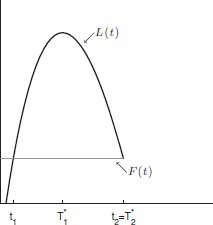
No clustering in the two-player game. The LPC brings the first investment forward to |$t_{1}$|⁠. Earlier preemption is not profitable: before |$t_{1}$|⁠, |$F\left( t \right)$| exceeds |$L\left( t \right)$|⁠. The figure is drawn for cost function |$c\left( t \right) = 2 \times {10^4}{e^{ - \left( {\alpha + r} \right)t}}$| for |$\alpha=0.24$|⁠, |$r = 0.1$|⁠, and flow profits |$\pi=(440,300)$|⁠.

Open in new tabDownload slide

The mechanism at work is the following. If unconstrained by strategic considerations, a single firm would like to invest at the stand-alone time |$T_1^*$|⁠. Also in the presence of an opponent, each firm would like to invest first, at |$T_1^*$|⁠. The opponent would then follow at |$T_2^*$|⁠. The leader would receive a higher payoff than the follower. This cannot be an equilibrium because the firm who takes the role of the follower could profitably deviate and preempt the opponent by investing at |$T_1^*-\varepsilon$|⁠. The presence of a second player introduces a Leader Preemption Constraint (LPC) on the time of the first investment: leader investment cannot take place at a time when earlier preemption is profitable. As a consequence, the first investment must occur strictly earlier than |$T_1^*$|⁠. In particular, it must occur weakly before the first intersection of the leader and follower payoff functions. Because the leader payoff function is increasing in that interval, the first investment will occur at the latest time that satisfies the LPC (i.e., the first intersection of the two curves).

3.2. The Three-Firm Game: When are the First Two Investments Clustered?

In this section, we move away from the two-player benchmark and illustrate the possibility of clustering in the context of a three-player game. As in the two-player game, the first investment must occur strictly earlier than |$T_1^*$|⁠. The key difference from the two-player game is that |$t_{1}$| is identified by the presence of two constraints. One is the LPC constraint discussed above. The second is what we call the Follower Preemption Constraint (FPC). The latter reflects the fact that the first investment is followed by a preemption race among the remaining two players. This race among followers determines an upper bound on the time of the first investment.

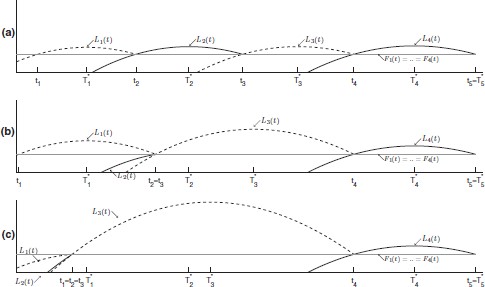
The aim of this section is twofold. First, we show that the first and second investments can be clustered or not clustered. Which case occurs depends on which of the two constraints on |$t_{1}$|⁠, the FPC or the LPC, is binding in equilibrium. Then, we examine how the model primitives determine which constraint is binding. We proceed by solving the game by backward induction. Figure 2 illustrates.

Figure 2.

Clustering versus no clustering. In all three panels, the third investment occurs at |$T_3^*$| and the second at the first intersection of |${L_2}\left( t \right)$| and |${F_2}\left( t \right)$|⁠. Duopoly profits decrease from Figure 2(a) to 2(c), delaying the second investment time |$t_{2}$|⁠. In Figures 2(a) and 2(b), |$t_2\le\ T_1^*$|⁠, so in the race to be first, |${F_1}\left( t \right)$| exceeds |${L_1}\left( t \right)$| before |$t_{2}$|⁠. Hence, only the FPC is binding and investments are clustered. Figure 2(b) represents the cutoff case with |${t_2} = T_1^*$|⁠. In Figure 2(c), |${t_2} > T_1^*$|⁠. Therefore, |$L_1(t)$| exceeds |${F_1}\left( t \right)$| before |$t_{2}$| and the LPC alone is binding. The cost function is the same as in Figure 1. Flow profits |$\pi$| are (440, 300, 150) for Figure 2(a), (440, 280.2, 150) for Figure 2(b), and (440, 240, 150) for Figure 2(c).

Open in new tabDownload slide

The Two-Firm Subgame

respectively. The threat of preemption guarantees that the first investment in the subgame must take place at the earliest time when |$L_2(t)=F_2(t)$|⁠. The second investment time in the game, |$t_{2}$|⁠, coincides with this intersection. The last investment occurs at |$T_3^*$|⁠.

The Follower Preemption Constraint

The conclusion above that the second investment occurs at the earliest intersection of |${L_1}\left( t \right)$| and |${F_2}\left( t \right)$| clearly assumes that the first investment must occur weakly before this intersection. We show by contradiction that this must be the case in equilibrium. Suppose that the first investment took place strictly later, at some time |$\tau \le T_3^*$|⁠. A two-firm subgame would then start at |$\tau$|⁠. Because |${L_2}(\tau)\gt {F_2}(\tau)$|⁠, both firms would prefer to be leader rather than follower in this subgame. They would both try to invest at |$\tau$|⁠; one would succeed and the other would invest later at |$T_3^*$|⁠. This cannot be an equilibrium because each of the last two investors receives a lottery between |${L_2}(\tau)$| and |${F_2}(\tau)$|⁠, while it could deviate and guarantee itself a payoff arbitrarily close to |${L_2}(\tau)$|⁠. Deviating by investing at |$\tau-\varepsilon$|⁠, a firm would be the first investor in the game. It would trigger a two-firm subgame in which one more investment would occur at |$\tau-\varepsilon$| and the last one at |$T_3^*$|⁠. Therefore, the deviator would receive a payoff of |${L_2}(\tau-\varepsilon)$|⁠.

We have established that the time of the first investment |$t_{1}$| is constrained by the presence of a preemption race in the ensuing two-firm subgame: to guarantee that there is rent equalization in this race, |$t_{1}$| must be no later than the first intersection of the leader and follower payoff curves of the two-firm subgame (i.e., |${L_2}(t)$| and |${F_2}(t)$|⁠). We call this the FPC. Because the second investment time |$t_{2}$| coincides with this intersection, we say that the FPC is binding in equilibrium if the first investment occurs exactly at |$t_{2}$|⁠, and not binding if it occurs strictly earlier than |$t_{2}$|⁠.¹⁵

The Leader Preemption Constraint

As in the two-player game, there is a LPC: the first investment cannot occur at a time such that earlier preemption is profitable, because otherwise any of the followers would have a profitable deviation. We say that the LPC on |$t_{1}$| is binding in equilibrium if given the subsequent investment times |$t_{2}$| and |$t_{3}$|⁠, |${L_1}\left( t \right) > {F_1}\left( t \right)$| for some |$t \lt {t_2}$|⁠. Otherwise, preempting the leader is never profitable, and we say that the LPC is not binding.

The Relationship between FPC and LPC

The FPC reflects the intensity of the follower preemption race that starts after the first investment: the more intense this race is, the earlier is the first intersection of |${L_2}\left( t \right)$| and |${F_2}\left( t \right)$| (i.e., the earlier |$t_{2}$| is). The LPC instead reflects the intensity of the race to be the first investor. These two constraints are not independent. The intensity of the race to be the first investor is a direct consequence of the intensity of the follower preemption race between the second and third investors. Hence, the LPC is directly affected by the FPC.

To capture this relationship between the two constraints, note that the more intense the follower preemption race is, the earlier |$t_{2}$| is, and hence the tighter the constraint on |$t_{1}$| imposed by the FPC becomes. At the same time, the earlier |$t_{2}$| is, the shorter the period becomes for which the first investor earns monopoly profits: early |$t_{2}$| makes the role of the first investor less desirable. Therefore, the more intense the follower preemption race is, the less intense is the race to be the first investor: the stronger the FPC, the weaker the LPC.

The key observation of our analysis is that for any given set of parameters, only one of the two constraints is binding, and which constraint is binding is equivalent to whether the first two investments are clustered or not. If the follower preemption race is sufficiently intense, only the FPC is binding, and investments are clustered. Otherwise, only the LPC is binding, and investment times are different. We discuss these two cases in the following, and illustrate them in Figure 2.

First, observe that the leader payoff |${L_1}\left( t \right)$| is strictly quasiconcave, and maximized at |$T_1^*$|⁠. By construction, it intersects |${F_1}\left( t \right)$| in |$t_{2}$|⁠. Which constraint is binding depends on the relative position of |$t_{2}$| with respect to |$T_1^*$|⁠. The intuition for this is that |$T_1^*$|⁠, being determined by |$\pi(1)$|⁠, reflects the desirability of the role of the first investor, and hence the strength of the LPC, while |$t_{2}$| reflects the strength of the FPC.

Case 1: |${t_2} \le T_1^*$| (Figures 2(a) and 2(b)). The LPC is not binding, because the follower payoff |${F_1}\left( t \right)$| exceeds the leader payoff |${L_1}\left( t \right)$| at any |$t \lt {t_2}$|⁠. The first investment occurs exactly at |$t_{2}$|⁠: the FPC is binding. The payoffs of all players are equalized. The first two investment times are clustered: |${t_1} = {t_2}$|⁠.

Case 2: |${t_2}{\mkern 1mu} > T_1^*$| (Figure 2(c)). The LPC is binding, because the leader payoff |${L_1}\left( t \right)$| exceeds the follower payoff |${F_1}\left( t \right)$| to the left of |$t_{2}$|⁠. The preemption race to be the first investor brings |$t_{1}$| forward to the earliest intersection of leader and follower payoffs. The payoffs of all players are equalized. The FPC, instead, is not binding. The first two investments are not clustered: |${t_1} \lt T_1^* \lt {t_2}$|⁠.

How Model Primitives Determine the Presence of a Cluster

As can be seen in Figure 2, whether Cases (1) or (2) will occur is equivalent to whether |${L_2}\left( t \right) - {F_2}\left( t \right)$|—the incentive to preempt in the two-player subgame that follows the first investment—is positive or negative when evaluated at |$T_1^*$|⁠.

In the cutoff case of Figure 2(b), the preemption incentive evaluated at |$T_1^*$| is zero: the first intersection of |${L_2}\left( t \right)$| and |${F_2}\left( t \right)$|⁠, which identifies |$t_{2}$|⁠, coincides exactly with |$T_1^*$|⁠. The follower preemption race is just intense enough to make the FPC binding and the LPC not binding. If, instead, the first intersection of|$\;{L_2}\left( t \right)$| and |${F_2}\left( t \right)$| occurs to the left of |$T_1^*$|⁠, as in Figure 2(a), then the preemption incentive |${L_2}\left( t \right) - {F_2}\left( t \right)$| evaluated at |$T_1^*$| is strictly positive. Conversely, if it occurs to the right of |$T_1^*$|⁠, as in Figure 2(c), then |${L_2}\left( t \right) - {F_2}\left( t \right)$| evaluated at |$T_1^*$| is strictly negative.

Recalling that |$T_1^*$| is a decreasing function of |$\pi(1)$| and |$T_3^*$| is a decreasing function of |$\pi(3)$|⁠, we observe that the preemption incentive evaluated at |$T_1^*$| is a function of the three profit parameters |$\pi(1)$|⁠, |$\pi(2)$|⁠, and |$\pi(3)$|⁠. For profit structures such that the preemption incentive (10) is nonnegative, the first two investments are clustered; for all other profit structures, clustering does not occur.

The preemption incentive (10) is monotonic in each of the profit parameters, |$\pi(1)$|⁠, |$\pi(2)$|⁠, and |$\pi(3)$|⁠. The intuition is captured by looking at how each of them affects the relative strength of the two constraints. First, the preemption incentive (10) is decreasing in |$\pi(1)$|⁠. Hence, starting from the cutoff case, by increasing |$\pi(1)$| we fall into Case (2) (no clustering). The intuition is that an increase in |$\pi(1)$| makes the role of leader of the three-player preemption race more attractive. Hence, the LPC becomes binding.

Next, consider |$\pi(2)$| and |$\pi(3)$|⁠. The preemption incentive (10) is increasing in |$\pi(2)$| and decreasing in |$\pi(3)$|⁠. Hence, starting from the cutoff case, increasing |$\pi(2)$| or decreasing |$\pi(3)$|⁠, there continues to be a cluster. The intuition is that an increase in |$\pi(2)$| or a decrease in |$\pi(3)$| makes the role of the second investor more attractive relative to the role of third investor. The preemption race among the followers becomes more intense, and this brings |$t_{2}$| forward. The FPC becomes stronger. At the same time, earlier |$t_{2}$| makes the role of the first investor less attractive, so the LPC becomes weaker.

In Section 3.4, we show that the intuition above can be translated into a sufficient condition for the presence of a cluster: given any pair |$\left( {\pi \left( 1 \right),\pi \left( 3 \right)} \right)$|⁠, if |$\pi(2)$| is sufficiently close to |$\pi(1)$|⁠, then the first and second investments are clustered.

3.3. The General Case: N Firms

In this section, we formalize and generalize our characterization of the equilibrium outcome of the game with three players to the general case of |$N$| players.

After the first |$j - 1$| investments have taken place, two constraints determine the next investment time |${t_j}$|⁠. First, the LPC: preempting the leader of the current subgame (i.e., the |$j$|th investor) by investing earlier than |${t_j}$| must not be profitable. Second, the FPC: |${t_j}$| must be weakly earlier than the time of the next investment |${t_{j + 1}}$|⁠, which is determined by the preemption race in the subgame played by the followers after the |$j$|th investment.¹⁶

Proposition 1 establishes that the equilibrium outcome of the game is unique, and that the rent-equalization result is preserved even for a general number of players. It allows us to construct a simple recursive algorithm with which to compute the equilibrium investment times and to determine the presence of clusters.

Proposition 1

The game admits a unique pure-strategy SPNE outcome, up to a permutation of players. The equilibrium has the following properties.

• (i)

  All players receive the same payoff.

• (ii)

  The|$j$|th and the|$\left( {j + 1} \right)$|th investments are clustered if and only if the|$\left( {j + 1} \right)$|th investment time|${t_{j + 1}}$|is weakly earlier than the|$j$|th stand-alone investment time|$T_j^*$|⁠.

In equilibrium, all players earn a payoff equal to that of the last investor: |$\left( {1/r} \right)\pi \left( N \right){e^{ - rT_N^*}} - c\left( {T_N^*} \right)$|⁠. The rent-equalization result of Fudenberg and Tirole (1985) extends to the |$N$|-player game because we assume that preinvestment payoffs are constant. This, in turn, implies that in each preemption race the follower payoff is independent of the exact time of earlier investments. While the game admits a unique equilibrium outcome in terms of investment times and equilibrium payoffs, the role taken by each investor in the investment sequence is not uniquely identified.¹⁷

Lemma 1 and Proposition 1 suggest the following simple recursive algorithm to compute the equilibrium investment times |$\left( {{t_1},{t_2},\ldots,{t_N}} \right)$| and determine the presence of clusters.

1. The last investment time is equal to the last stand-alone investment time: |${t_N} = T_N^*$|⁠.

2. For |$j \lt N$|⁠, (i) if |${t_{j + 1}} \le T_j^*$|⁠, then there is a cluster: |${t_j} = {t_{j + 1}}$|⁠; (ii) if |${t_{j + 1}} > T_j^*$|⁠, then |${t_j} \lt {t_{j + 1}}$|⁠, and |${t_j}$| solves the rent-equalization condition

   $${L_j}\left( t \right) - {F_j}\left( t \right) = \pi \left( j \right)\mathop \int \nolimits_{{t_j}}^{{t_{j + 1}}} {e^{ - rs}}ds - c\left( {{t_j}} \right) + c\left( {{t_{j + 1}}} \right) = 0$$

   where |${L_j}\left( t \right)$| and |${F_j}\left( t \right)$| are defined analogously to |${L_1}\left( t \right)$| and |${F_1}\left( t \right)$|⁠.¹⁸

Case (i) is analogous to Case (1) in Section 3.2: the FPC alone is binding. Case (ii) is analogous to Case (2) in Section 3.2: the LPC alone is binding.

Proposition 1 has two implications that go beyond the features of the three-player example. First, for |$N > 3$|⁠, clusters can include more than two simultaneous investments. For example, suppose that the preemption race for the role of the |$\left( {j + 1} \right)$|th investor is sufficiently intense that not only |${t_{j + 1}} \lt T_j^*$|⁠, but also |${t_{j + 1}} \lt T_{j - 1}^* \lt T_j^*$|⁠; in this case, the |$\left( {j - 1} \right)$|th, |$j$|th, and |$\left( {j + 1} \right)$|th investments will be clustered. In Section 3.4, we illustrate how model primitives affect the size of a cluster.

Second, clusters can occur not only at the beginning, but at any point of the investment sequence, except for the last.¹⁹

3.4. The Condition for a Cluster

In Section 3.2, we illustrated the mechanism that leads to clustered investments in the special case of |$N = 3$|⁠. We introduced the LPC and the FPC and provided an intuitive discussion of how the model parameters affect these two constraints and determine the presence or absence of a cluster. In this section, we formally investigate how the mechanism illustrated in Section 3.2 relates to the model primitives. More precisely, we ask under which condition on the parameters of the model are two or more subsequent investments clustered, at any point in the investment sequence.

The answer is that they are clustered if the associated flow profits are sufficiently close. To obtain this result, we first argue that whether two subsequent investments are clustered or not depends only on a subvector of the profit structure |${\mathbf{\pi }}$|⁠. Second, we present a comparative statics result relating investment times and flow profits. Third, we identify a sufficient condition on the profit structure for a cluster of two or more investments. Figure 3 illustrates the analysis.

We start by observing that the equilibrium characterization in Proposition 1 implies the following.

Remark 1

The condition for a cluster of two subsequent investments is independent of the flow-profit parameters associated with earlier investments.

Proposition 1 states that whether the |$j$|th and |$\left( {j + 1} \right)$|th investments are clustered is determined by the comparison of the stand-alone investment time |$T_j^*$| and the |$\left( {j + 1} \right)$|th equilibrium investment time |${t_{j + 1}}$|⁠. Hence, the condition for a cluster depends only on the flow-profit parameters affecting |$T_j^*$| and |${t_{j + 1}}$|⁠. As illustrated in Section 2.3, |$T_j^*$| depends only on the flow-profit parameter |$\pi \left( j \right)$|⁠. To see which profit parameters determine |${t_{j + 1}}$|⁠, consider the algorithm identifying the equilibrium investment times. The last investment occurs at |${t_N} = T_N^*$|⁠, and hence it depends only on one flow-profit parameter, |$\pi \left( N \right)$|⁠. The previous investment time |${t_{N - 1}}$| depends on |$\pi \left( {N - 1} \right)$| and on the flow-profit parameters that affect |${t_N}$| (i.e., on |$\pi \left( N \right)$|⁠). Continuing to apply the algorithm, it follows that |${t_{j + 1}}$| depends only on |$\pi \left( {j + 1} \right)$| and on the flow-profit parameters that affect later investments (i.e., on the vector |$\left( {\pi \left( {j + 1} \right),\pi \left( {j + 2} \right),\ldots,\pi \left( N \right)} \right)$|⁠).

We now present a comparative statics result that will play a key role in the construction of the sufficient condition for a cluster.

Proposition 2

Each equilibrium investment time is decreasing in the associated flow profit.

For expositional purposes, consider a profit structure such that the equilibrium investment times |${t_j}$| and |${t_{j + 1}}$| are different. An increase in |$\pi \left( j \right)$| makes the role of the |$j$|th investor more profitable. Rent equalization requires that the |$j$|th investor receives the same equilibrium payoff as the |$\left( {j + 1} \right)$|th investor. The latter is unaffected by the increase in |$\pi \left( j \right)$|⁠. Hence, in equilibrium, an increase in |$\pi \left( j \right)$| has to be offset by an increase in the investment cost. This implies bringing |${t_j}$| forward, because the investment cost is decreasing in time.

The monotonicity of equilibrium investment times in flow profits leads to our main result. An increase in |$\pi \left( j \right)$| brings |${t_j}$| forward. For sufficiently large |$\pi \left( j \right)$| (i.e., for |$\pi \left( j \right)$| sufficiently close to |$\pi \left( {j - 1} \right)$|⁠), |${t_j}$| occurs at a time earlier than |$T_{j - 1}^*$|⁠. This results in a cluster of the |$j$|th and |$\left( {j - 1} \right)$|th investments. By the same mechanism, if |$\pi \left( j \right)$| is sufficiently close to |$\pi \left( {j - 2} \right)$|⁠, the investment time |${t_j}$| is brought forward to a time even earlier than |$T_{j - 2}^*$|⁠. This results in a cluster of three investments: |${t_{j - 2}} = {t_{j - 1}} = {t_j}$|⁠. Figure 3 illustrates this mechanism. More generally, for any |$j \in \left\{ {2,\ldots,N - 1} \right\}$| and |$k \in \left\{ {1,\ldots,j - 1} \right\}$|⁠, the sufficient condition for a cluster of two or more investments is as follows.

Proposition 3

If|$\pi \left( j \right)$|is sufficiently close to|$\pi \left( {j - k} \right)$|⁠, then the|$j$|th investment is clustered with the previous|$k$|investments.

To capture the intuition for this result, consider the simplest case of a cluster of two investments. Suppose that the parameter values are such that the |$j$|th investment is not clustered with the previous one. Consider an increase in the flow profits |$\pi \left( j \right)$|⁠. How does it affect the preemption incentives in the game? The same reasoning as illustrated in Section 3.2 and Figure 2 for |$N = 3$| and |$j = 2$| applies here. The |$\left( {j - 1} \right)$|th investment time is determined by the FPC and the LPC. Everything else equal, an increase in |$\pi \left( j \right)$| makes the role of the |$j$|th investor more attractive. Therefore, the follower preemption race in the subgame starting after the |$\left( {j - 1} \right)$|th investment becomes more intense. This brings forward the investment time |${t_j}$|⁠, which constitutes the upper bound on the investment time |${t_{j - 1}}$| stemming from the FPC. In turn, an earlier investment time |${t_j}$| makes the role of the |$\left( {j - 1} \right)$|th investor less attractive, so the preemption race for the role of the |$\left( {j - 1} \right)$|th investor is less intense, and the LPC becomes weaker. The natural question is whether it is possible to increase |$\pi \left( j \right)$| to such an extent that the FPC becomes binding and the LPC becomes not binding. Proposition 3 provides a positive answer, as follows. For any value of the remaining primitives of the model, it is always possible to find |$\pi \left( j \right)$| strictly smaller than |$\pi \left( {j - 1} \right)$| but sufficiently close to it, such that the FPC is binding, the LPC is not binding, and the |$j$|th investment is clustered with the previous one.

Figure 3.

The size of a cluster. In all three panels, |$N = 5$|⁠, the cost function is |$c\left( t \right) = 2 \times {10^4}{e^{ - \left( {\alpha + r} \right)t}}$|⁠, with |$\alpha = 0.4$| and |$r = 0.1$|⁠, and the flow profits |$\left( {\pi \left( 1 \right),\pi \left( 2 \right),\pi \left( 4 \right),\pi \left( 5 \right)} \right)$| are (340, 320, 280, 270). Triopoly profits |$\pi(3)$| increase from 300 in Figure 3(a) to 308 in Figure 3(b), and to 316 in Figure 3(c). The investment times |$t_{4}$| and |$t_{5}$| are unaffected by this increase (Remark 1). Also, |$T_1^*$| and |$T_2^*$| are the same in all panels. In Figure 3(a), |$T_1^* \lt T_2^* \lt {t_3}$| and no cluster occurs. In Figures 3(b) and 3(c), the larger |$\pi(3)$| brings the third investment time |$t_{3}$| forward (Proposition 2). In Figure 3(b), |$\pi(3)$| is sufficiently close to |$\pi(2)$| such that |$T_1^* \lt {t_3} \lt T_2^*$| and the second and third investments are clustered. In Figure 3(c), a further increase of |$\pi(3)$| makes it sufficiently close to |$\pi(1)$|⁠, such that |${t_3} \lt T_1^* \lt T_2^*$| and the first three investments are clustered (Proposition 3).

Open in new tabDownload slide

We conclude with a remark regarding what can be learned about profits, when data on the timing of investments are observed. Our result says that clustering of entry or adoption times does not imply that payoffs are not declining in rival investment. If investment times are generated by a preemption game and clustering is observed, this implies a bound on the decline in profits due to rival investment. In the case where only time-aggregated information is available, for instance in the form of annual data, bounds could nevertheless be obtained but would be less informative the higher the level of temporal aggregation.

Consider the case |$N = 3$|⁠. If we the investment cost function and the interest rate, then we can find |$\pi(3)$| because it is the unique solution to the stand-alone problem in (2) given |$T_3^*$|⁠. Knowing |$T_3^*$| and |$\pi(3)$|⁠, we can find |$\pi(2)$| by plugging the observed |$t_{2}$| into the rent-equalization condition |${L_2}\left( {{t_2}} \right) = {F_2}\left( {{t_2}} \right)$|⁠. If |${t_1} \lt {t_2}$|⁠, we can repeat the same procedure and use |${L_1}\left( {{t_1}} \right) = {F_1}\left( {{t_1}} \right)$| to find |$\pi(1)$|⁠. If, instead, |${t_1} = {t_2}$| (i.e., there is a cluster), we can infer that |$\pi(1)$| must be small enough, such that |$T_1^* > {t_2}$|⁠. Thus, an upper bound |$\bar \pi \left( 1 \right)$| for |$\pi(1)$| as a function of |$t_{2}$| can be obtained. This implies that |$\pi(1)$| must lie in the interval |$\left[ {\pi \left( 2 \right),\bar \pi \left( 1 \right)} \right]$|⁠.

4. Conclusions

In this paper, we have analyzed an |$N$|-player preemption game in which the players’ payoffs before investing are constant (and normalized to zero). The game has a unique equilibrium outcome, and the rent-equalization result of the two-player game analyzed by Fudenberg and Tirole (1985) is preserved.

We find that clusters of simultaneous investments are possible. When the preemption race among late investors is very intense, the preemption incentive for earlier investors is reduced. If this effect is sufficiently strong, two or more investments occur at the same time. We characterize a sufficient condition on the model primitives for two or more investments to be clustered: the flow profits of subsequent investments must be sufficiently close. Our results imply that the observation of investment clustering in preemptive environments need not reflect informational spillovers, positive externalities, or coordination failures. Instead, clustering implies a bound on the decline in profits due to rival investment.

Acknowledgments

For comments and suggestions, we thank Dirk Bergemann, Alberto Galasso, Paul Heidhues, Paul Klemperer, three anonymous referees, and seminar participants at Bonn, City, Essex, Helsinki, Indiana, Leicester, LSE, Manchester, Mannheim, Naples, Oxford, Pompeu Fabra, Toulouse, Warwick, Yale, Zurich, EARIE 2006, SAET 2007, and the 14th WZB–CEPR Conference on Markets and Politics. Financial support from the ESRC under grant RES-000-22-1906 is gratefully acknowledged. Schmidt-Dengler is also affiliated with CEPR, CESifo, and ZEW.

Appendix

Claim A.1

For any |$j \in \left\{ {1,2,\ldots,N} \right\}$|⁠:

• (a)

  the function|${f_j}\left( t \right)$|is strictly quasiconcave in|$t$|;

• (b)
  it admits a unique global maximum in|$T_j^*$|⁠, defined as the solution to

  $$f_j^\prime \left( t \right) = 0 \Leftrightarrow - \pi \left( j \right){e^{ - rt}} - c'\left( t \right) = 0;$$
• (c)

  |${f_j}\left( {T_j^*} \right) > 0$|and|$T_j^* \lt T_{j'}^*$|for|$j \lt j'$|⁠.

Proof

Part (a). We prove that the function is strictly quasiconcave, by showing that in every critical point of the function the second derivative is strictly negative. The first derivative |$f_j^\prime \left( t \right)$| is equal to |$\left( { - \pi \left( j \right){e^{ - rt}} - c'\left( t \right)} \right)$| and the second derivative |$f_j^{\prime \prime }\left( t \right)$| is equal to |$\left( {r\pi \left( j \right){e^{ - rt}} - c''\left( t \right)} \right)$|⁠. Using |$f_j^\prime \left( t \right) = 0$|⁠, we can rewrite |$f_j^{\prime \prime }$| evaluated at any critical point as

$$f_j^{\prime \prime }\left( t \right) = - c'\left( t \right)r - c''\left( t \right).$$

(A.1)

By Assumption 2, |${e^{rt}}\left( {c'\left( t \right) + rc\left( t \right)} \right) \lt 0$| and |${e^{rt}}\left( {2c'\left( t \right)r + c\left( t \right){r^2} + c''\left( t \right)} \right) > 0$|⁠. Together, these two inequalities imply that expression (A.1) is negative.

Part (b). We prove that the first-order condition |$f_j^\prime \left( t \right) = 0$| admits a solution and hence characterizes the unique global maximum of the function by showing that |$f_j^\prime \left( t \right)$| is positive at zero and negative for sufficiently large values of |$t$|⁠. Assumptions 1 and 3 guarantee that |${f_j}\left( t \right)$| is negative at zero and positive at a later time. Quasiconcavity then implies that |$f_j^\prime \left( 0 \right) > 0$|⁠. Moreover, because |${f_j}\left( t \right)$| is continuous and is either always increasing or single peaked, it admits a limit as |$t$| goes to infinity. This limit must be greater than or equal to zero by Assumption 3(ii). It must also be smaller than or equal to zero because |${\lim _{t \to + \infty }}{f_j}\left( t \right) = - {\lim _{t \to + \infty }}c\left( t \right)$|⁠. Hence, the only possible candidate limit is zero. However, if that is the case, because the function is positive from some |$\tau$| onwards, as |$t$| goes to infinity it must approach zero from above. Hence, it must be decreasing for |$t$| sufficiently large. Therefore, we conclude that the function |${f_j}\left( t \right)$| admits a critical point.

Part (c). Assumptions 2(i) and 3(ii) imply that |${f_N}\left( t \right)$| is strictly positive for any |$t \ge T_N^*$|⁠. Thus, Assumption 1(ii) implies that |${f_j}\left( {T_j^*} \right) > 0$| for all |$j$|⁠.

Finally, note that by the implicit function theorem

$$\frac{{\partial T_j^*}}{{\partial \pi \left( j \right)}} = - \frac{{ - {e^{ - rT_j^*}}}}{{f_j^{\prime \prime }\left( {T_j^*} \right)}} \lt 0,$$

where the inequality holds because |$T_j^*$| is a maximum, and hence the denominator is negative. Therefore, Assumption 1(ii) implies that |$T_1^* \lt T_2^* \lt \ldots \lt T_N^*$|⁠. □

Proof of Lemma 1

Assumptions 1(ii) and 3(i) guarantee that there is no investment at time zero; the cost of investing immediately is higher than the maximum amount of profits a firm can obtain in this game.

The proof of the result that all firms invest in finite time, and that the last investment takes place at the stand-alone investment time |$T_N^*$|⁠, is split into two parts. First, we show that in equilibrium, at any decision node with one active firm and calendar time |$t$|⁠, the firm plays “wait” if |$t \lt T_N^*$| and “invest” otherwise. Then, we show that in any decision node with |$t \ge T_N^*$| any number of active firms play “invest”.

The payoff of a single active firm from investing at time |$t$| is |${f_N}\left( t \right)$|⁠, defined in equation (2). From Claim A.1, |${f_N}\left( t \right)$| has a strict global maximum in |$T_N^*$| and its maximum value is strictly positive. Therefore, a single active firm will optimally play “wait” if |$t \lt T_N^*$| and “invest” otherwise.

Next, consider decision nodes with |$t \ge T_N^*$| and two active firms. We show that both firms must invest exactly at |$t$|⁠.

First, suppose that at |$t$| they both play “invest”. By Assumption 4, only one of them succeeds and the game enters a subgame with one active firm. As we proved above, this firm invests immediately, so both firms invest at time |$t$| and receive payoff |${f_N}\left( t \right)$|⁠. No firm has an incentive to deviate from these strategies. With two active firms, deviating and playing “wait” would not change the outcome, nor the deviator’s payoff. The non-deviating firm would invest immediately. The game would therefore enter a subgame with one active firm in which the deviator would optimally invest immediately, as we proved above.

Next, suppose that at time |$t$| only one of the two active firms plays “invest”. The outcome is again that both firms invest at |$t$|⁠, because after one firm invests the game enters a subgame with one active firm, in which it is optimal to invest immediately. No firm has an incentive to deviate from these strategies. The firm who plays “wait” has no incentive to deviate because the outcome, hence its payoff, would be unchanged. Now, suppose that the firm who plays “invest” deviates. It would receive a payoff of either zero, if it never invests, or |${f_N}\left( \tau \right)$|⁠, if it invests at some |$\tau > t$|⁠. Because |${f_N}\left( \cdot \right)$| is positive and strictly decreasing in the interval considered, the deviation is not profitable.

Finally, suppose that at time |$t$| both firms play “wait”. The argument immediately above shows that each firm would be better off by deviating and playing “invest” at |$t$|⁠.

Repeating the same argument for |$\ell = 3,\ldots,N$|⁠, it follows that in any SPNE, at any decision node with |$t \ge T_N^*$| and any number |$\ell$| of active firms, at least one of these plays “invest”, and the claim follows immediately. □

Proof of Proposition 1

Through a series of Lemmata, we show that the game admits a unique SPNE outcome, and we characterize its properties. The proof is articulated in the following steps.

Denote by |${t_j}$| the SPNE investment time of the |$j$|th investor, for |$j \in \left\{ {1,\ldots,N} \right\}$|⁠. In Definition A.1, we introduce three functions: |${L_j}\left( t \right)$|⁠, |${F_j}\left( t \right)$|⁠, and their difference |${D_j}\left( t \right)$|⁠. In Lemmata A.1 and A.2, we characterize their properties. Over a well-defined subset of their domain, |${L_j}\left( t \right)$| and |${F_j}\left( t \right)$| can be interpreted as the payoff of the |$j$|th investor and the |$\left( {j + 1} \right)$|th investor, respectively, if the |$j$|th investment takes place at |$t$| and the following investments take place at |${t_{j + 1}},\ldots,{t_N}$|⁠, respectively. In the definition, the existence and uniqueness of the SPNE investment times are assumed. In the development of the proof, they will be proved. The existence and uniqueness of |${t_N} = T_N^*$| have been proved in Lemma 1.

In Lemma A.3, we establish that in any subgame with one active firm, it plays “wait” before |$T_N^*$| and “invest” from |$T_N^*$| on. In Lemma A.4, we prove that there exists a time |${T_{N - 1}} \lt T_N^*$| in which |${L_{N - 1}}\left( {{T_{N - 1}}} \right) = {F_{N - 1}}\left( {{T_{N - 1}}} \right)$|⁠, and in Lemma A.5 we prove that this is the unique |$\left( {N - 1} \right)$|th equilibrium investment time. Therefore, the equilibrium payoff of the last two investors is the same.

Finally, in Lemmata A.6, A.7, and A.8, we identify the algorithm for the construction of the equilibrium investment times |${t_j}$| for |$j \in \left\{ {1,\ldots,N - 2} \right\}$|⁠, identifying the condition for clustering, and we prove that rent equalization holds in equilibrium for all players. The argument is based on the induction principle. Lemma A.6 proves that there exists an algorithm to identify the unique |${t_{N - 2}}$|⁠, given |${t_{N - 1}}$| and |${t_N}$|⁠, and that the equilibrium payoff of the last three investors is the same. Lemma A.7 shows that if an analogous algorithm can be used to identify a unique value of |${t_{N - l}}$|⁠, given |${t_{N - l + 1}},\ldots,{t_N}$|⁠, and rent equalization holds for the last |$l$| players, then the same algorithm identifies a unique value for |${t_{N - l - 1}}$|⁠, given |${t_{N - l}},\ldots,{t_N}$|⁠, and rent equalization holds for the last |$l + 1$| players. Lemma A.8 applies the induction principle to prove that the algorithm can be used to construct the SPNE investment times |${t_1},\ldots,{t_{N - 2}}$| and rent equalization holds for all players. □

Definition A.1

For each |$j \in \left\{ {1,\ldots,N - 1} \right\}$|⁠, we define the following three functions over the interval |$\left[ {0,T_N^*} \right]$|⁠:

$$\begin{align} & \begin{matrix} {{L}_{j}}\left( t \right) & \equiv & \pi \left( j \right){\mathop \int \nolimits_{t}^{{{{t}_{j+1}}}}}\,{{e}^{-rs}}ds+{\mathop \sum \limits_{m=j+1}^{{N}}}\,\pi \left( m \right){\mathop \int \nolimits _{{{t}_{m}}}^{{{{t}_{m+1}}}}}\,{{e}^{-rs}}ds-c\left( t \right) \\\end{matrix} \\ & \begin{matrix} {{F}_{j}}\left( t \right) & \equiv & {\mathop \sum \limits_{m=j+1}^{{N}}}\,\pi \left( m \right){\mathop \int \nolimits_{{{t}_{m}}}^{{{{t}_{m+1}}} }}\,{{e}^{-rs}}ds-c\left( {{t}_{j+1}} \right) \\\end{matrix} \\ & \begin{matrix} {{D}_{j}}\left( t \right) & \equiv & {{L}_{j}}\left( t \right)-{{F}_{j}}\left( t \right)=\pi \left( j \right){\mathop \int \nolimits_{t}^{{{{t}_{j+1}}}}}\,{{e}^{-rs}}ds-c\left( t \right)+c\left( {{t}_{j+1}} \right) \\\end{matrix} \\ \end{align}$$

where |${t_{N + 1}} \equiv + \infty$|⁠.

Notice that |${F_j}\left( t \right)$| is constant with respect to |$t$|⁠.

Lemma A.1

• (i)

  The function|${D_j}\left( t \right)$|attains a unique global maximum in|$T_j^*$|⁠, for|$j \in \left\{ {1,\ldots,N - 1} \right\}$|⁠.

• (ii)

  |${D_j}\left( {T_j^*} \right) \ge 0$|for|$j \in \left\{ {1,\ldots,N - 1} \right\}$|⁠.

Proof

Part (i). Notice that

$${D_j}\left( t \right) = \pi \left( j \right)\mathop \int \nolimits_t^{{t_{j + 1}}} {e^{ - rs}}ds - c\left( t \right) + c\left( {{t_{j + 1}}} \right)$$

(A.2)

and |${f_j}\left( t \right)$| as defined in equation (2) differ by a finite constant. By Claim A.1, |${f_j}\left( t \right)$| attains a unique global maximum in |$T_j^*$|⁠, hence the same is true for |${D_j}\left( t \right)$|⁠.

Part (ii). Because |${D_j}\left( {{t_{j + 1}}} \right) = 0$| and |$T_j^*$| is the unique global maximizer, it holds that |${D_j}\left( {T_j^*} \right) \ge 0$|⁠. □

Lemma A.2

• (i)

  If|$T_j^* \le {t_{j + 1}}$|⁠, then|$\exists {T_j} \in \left( {0,T_j^*} \right]$|⁠, such that|${D_j}\left( {{T_j}} \right) = 0$|⁠.

• (ii)

  If|$T_j^* > {t_{j + 1}}$|⁠, then|${D_j}\left( t \right) \lt 0$|and|$D_j^\prime \left( t \right) > 0 \forall t \lt {t_{j + 1}}$|⁠.

Proof

Because |${D_j}\left( t \right)$| and |${f_j}\left( t \right)$| differ by a finite constant, Claim A.1 implies that |${D_j}\left( t \right)$| is strictly quasiconcave. Also, |${D_j}\left( 0 \right) \lt 0$|⁠, because

$$\begin{array}{*{35}{l}} {{L}_{j}}\left( 0 \right) & = & \pi \left( j \right)\int_{0}^{{{t}_{j+1}}}{{{e}^{-rs}}ds+\underset{m=j+1}{\overset{N}{\mathop \sum }}\,\pi \left( m \right)}\int_{{{t}_{m}}}^{{{t}_{m+1}}}{{{e}^{-rs}}ds-c\left( 0 \right)} \\ {} & \lt & \frac{\pi \left( 1 \right)}{r}-c\left( 0 \right) \\ {} & \lt & 0 \\ {} & \le & {{V}^{j+1}}\left( {{t}_{1}},\ldots,{{t}_{N}} \right) \\ {} & = & \underset{m=j+1}{\overset{N}{\mathop \sum }}\,\pi \left( m \right)\int_{{{t}_{m}}}^{{{t}_{m+1}}}{{{e}^{-rs}}ds-c\left( {{t}_{j+1}} \right)} \\ {} & = & {{F}_{j}}\left( 0 \right). \\ \end{array} $$

Here, the second inequality holds by Assumption 3(i) and the third because no firm receives a negative payoff in equilibrium, because it could always delay investment indefinitely, thus ensuring a payoff of zero. Moreover, |${D_j}\left( {{t_{j + 1}}} \right) = 0$|⁠. Therefore, two cases are possible: (i) |$T_j^* \le {t_{j + 1}}$|⁠, in which case |$\exists {T_j} \in \left( {0,T_j^*} \right]$|⁠, such that |${D_j}\left( {{T_j}} \right) = 0$|⁠, and |${D_j}\left( t \right) > 0$| in the interval |$t \in \left( {{T_j},{t_{j + 1}}} \right)$|⁠; (ii) |$T_j^* > {t_{j + 1}}$|⁠, in which case |${D_j}\left( t \right) \lt 0$| and |$D_j^\prime \left( t \right) > 0 \forall t \lt {t_{j + 1}}$|⁠. □

In the next lemma, we analyze decision nodes with one active firm.

Lemma A.3

In equilibrium, if at time|$t$|there is one active firm, it plays “wait” if|$t \lt T_N^*$|and“invest” if|$t \ge T_N^*$|⁠.

Proof

The result follows immediately from the proof of Lemma 1. □

In the next lemma, we show that for the case |$j = N - 1$|⁠, case (i) of Lemma A.2 applies.

Lemma A.4

|$T_{N - 1}^* \lt {t_N}$||${\mkern 1mu} = T_N^*$|and there is|${T_{N - 1}} \lt T_{N - 1}^* \lt T_N^*$|⁠, such that|${D_{N - 1}}\left( {{T_{N - 1}}} \right) = 0$|⁠.

Proof

|$T_{N - 1}^* \lt T_N^*$| by Claim A.1 and |${t_N}$||${\mkern 1mu} = T_N^*$| by Lemma 1. The rest of the statement follows from Lemma A.2. □

In the next lemma, we show that the |$\left( {N - 1} \right)$|th equilibrium investment time is |${T_{N - 1}}$|⁠.

Lemma A.5

In equilibrium, it holds that (i) in all subgames starting at|$t \in \left[ {{T_{N - 1}},T_N^*} \right)$|⁠, if there are|$n > 1$|active firms,|$n - 1$|investments take place at|$t$|; (ii) in all subgames starting at|$t \in \left[ {0,{T_{N - 1}}} \right)$|⁠, if there are|$n = 2$|active firms, each of them plays “wait”; (iii)|${t_{N - 1}} = {T_{N - 1}}$|and the equilibrium payoff of the last two investors is the same.

Proof

Part (i). We start from the observation that if |$t$| belongs to the interval |$\left( {{T_{N - 1}},T_N^*} \right)$|⁠, then |${D_{N - 1}}\left( t \right) > 0$|⁠, while if |$t = {T_{N - 1}}$|⁠, then |${D_{N - 1}}\left( t \right) = 0$|⁠. The proof now consists of three steps. Step (a) identifies two strategy profiles that generate the same outcome and constitute an equilibrium for any subgame with |$n > 1$| active firms starting at |$t \in \left( {{T_{N - 1}},T_N^*} \right)$|⁠. Step (b) rules out any other candidate equilibrium for subgames with |$n > 1$| active firms starting at |$t \in \left( {{T_{N - 1}},T_N^*} \right)$|⁠. Step (c) considers subgames with |$n > 1$| active firms starting exactly at |$t = {T_{N - 1}}$|⁠.

(a) We first show that it is an equilibrium for any subgame with |$n > 1$| active firms starting at |$t \in \left( {{T_{N - 1}},T_N^*} \right)$| that each active firm plays “invest” at all times |$\tau \ge t$|⁠, unless it is the only active firm.²⁰ The outcome of this candidate equilibrium is that all active firms try to invest immediately at |$t$|⁠, until only one is left. The last active firm will then wait to invest until time |$T_N^*$| by Lemma A.3. The associated payoff for each firm is a lottery between |${L_{N - 1}}\left( t \right)$| and |${F_{N - 1}}\left( t \right)$| with probability |$1/n$| assigned to |${F_{N - 1}}\left( t \right)$|⁠.

Suppose one firm deviates and plays “wait” at |$t$|⁠, although it is not the only active firm. We show that any deviation involving the play of “wait” at |$t$| when one or more other firms are active gives a smaller payoff than the payoff in the candidate equilibrium. We need to distinguish three possible classes of deviations according to the specific circumstances when the deviator plays “wait”.

First, consider the class of deviations in which the firm plays “wait” at |$t$| if at least one other firm is active. At |$t$|⁠, the |$n - 1$| non-deviating firms follow the given strategies, and hence |$n - 1$| investments occur at |$t$| and the deviating firm becomes the last active firm. By Claim A.1, the most profitable deviation in this class is the one in which the deviator later invests at |$T_N^*$|⁠. The associated payoff is |${F_{N - 1}}\left( t \right)$|⁠, which is smaller than the lottery between |${L_{N - 1}}\left( t \right)$| and |${F_{N - 1}}\left( t \right)$| given by the candidate equilibrium.

Second, consider the class of deviations in which the firm plays “wait” at |$t$| if the number of active firms is different from |$n - l$|⁠, for a given |$l$| such that |$n - l > 1$|⁠. At |$t$|⁠, the |$n - 1$| nondeviating firms follow the given strategies. The deviation outcome is the following. First, the |$n - 1$| nondeviating firms will play “invest” until |$l$| investments will occur. Then, when there are |$n - l$| active firms left, all of them, including the deviator, will play “invest”. With probability |$1/\left( {n - l} \right)$|⁠, the deviating firm will successfully invest and receive payoff |${L_{N - 1}}\left( t \right)$|⁠. With the complementary probability, the deviating firm will fail to invest. In the latter case, the game enters a subgame with |$n - l - 1$| active firms in which all firms except for the deviator will continue to play “invest” at |$t$|⁠, until the deviator is the only active firm. By Claim A.1, we can again identify the most profitable deviation within this class: If the outcome of the randomization device is such that the deviator is unsuccessful in investing when there are |$n - l$| active firms, the deviator will be the last active firm remaining. In this case, it should then invest at |$T_N^*$|⁠. Hence, the highest payoff in this class of deviations is a lottery between |${L_{N - 1}}\left( t \right)$| and |${F_{N - 1}}\left( t \right)$|⁠, with probability |$\left( {n - l - 1} \right)/\left( {n - l} \right)$| assigned to |${F_{N - 1}}\left( t \right)$|⁠, which is worse than the lottery deriving from the candidate equilibrium strategies because |$\left( {n - l - 1} \right)/\left( {n - l} \right) > 1/n$|⁠.

Third, an analogous argument shows that the class of deviations in which the firm plays “wait” at |$t$| if the number of active firms is different from |$n - l$|⁠, for a set of at least two integers |$l$|⁠, such that |$n - l > 1$| for every |$l$|⁠, the highest possible payoff is a lottery between |${L_{N - 1}}\left( t \right)$| and |${F_{N - 1}}\left( t \right)$|⁠, which assigns to |${F_{N - 1}}\left( t \right)$| a higher probability than the lottery deriving from the candidate equilibrium strategies.

(b) Next, we show that if |$t$| belongs to the interval |$\left( {{T_{N - 1}},T_N^*} \right)$|⁠, no strategy profile different from the ones presented in (a) constitutes an equilibrium. We need to rule out two classes of strategy profiles: one in which at |$t$|⁠, with |$n$| active firms, one or more firm plays “wait” and one or more firms play “invest”, and one in which all active firms play “wait” in an interval with positive measure starting at |$t$|⁠.

We develop the argument by induction. First, we show that it holds for |$n = 2$| active firms. Then, we show that if it holds for |$n = m \ge 2$|⁠, then it holds for |$n = m + 1$|⁠. Finally, we conclude that it holds for any |$n \ge 2$| by the induction principle.

The statement holds for|$\;n = 2$|⁠. We consider two classes of strategy profiles: one in which at |$t$|⁠, with two active firms, one firm plays “wait” and the other plays “invest”, and one in which both active firms play “wait” in an interval with positive measure starting at |$t$|⁠.

No strategy profile in the first class can be an equilibrium, because the firm who plays “wait” ends up being the last active firm in the game, thus receiving a payoff no larger than |${F_{N - 1}}\left( t \right)$|⁠, while it could profitably deviate by playing “invest” and receiving a lottery between |${L_{N - 1}}\left( t \right)$| and |${F_{N - 1}}\left( t \right)$|⁠.

Strategy profiles in the second class imply that the first investment in the subgame occurs strictly later than |$t$| and weakly before |$T_N^*$| (by Lemma 1), at some |$\tau \in \left( {t,T_N^*} \right]$|⁠, and the second at |$T_N^*$| by Lemma A.3. The strategy profiles for which both firms play “invest” at |$\tau$| cannot be an equilibrium because both firms get |$\left( {1/2} \right)\left( {{L_{N - 1}}\left( \tau \right) + {F_{N - 1}}\left( \tau \right)} \right)$| while each of them could deviate by investing at |$\tau - \varepsilon$| and receiving |${L_{N - 1}}\left( {\tau - \varepsilon } \right)$|⁠. By continuity, |$\exists \varepsilon > 0$| small enough that this is profitable. The strategy profiles for which only one of the two firms plays “invest” at |$\tau$| cannot be an equilibrium. The firm who does not invest at |$\tau$| must invest at |$T_N^*$| by Lemma A.3, thus receiving |${F_{N - 1}}\left( \tau \right)$|⁠. It could profitably deviate by investing at |$\tau - \varepsilon$| and getting |${L_{N - 1}}\left( {\tau - \varepsilon } \right)$|⁠.

If the statement holds for|$m$|⁠, it holds for|$m + 1$|⁠. Again, we need to consider two classes of strategy profiles: one in which at time |$t$|⁠, with |$m + 1$| active firms, only |$\nu \lt m + 1$| play “invest”, with |$\nu > 0$|⁠, and one in which all active firms play “wait” in an interval with positive measure starting at |$t$|⁠.

No strategy profile in the first class can be an equilibrium. At |$t$|⁠, one of the |$\nu$| firms will successfully invest and the game will enter a subgame with |$m$| active firms and calendar time |$t$|⁠. Given the assumption that the statement holds for |$n = m$|⁠, in such a subgame all |$m$| active firms invest immediately until only one is left, which invests at |$T_N^*$|⁠. Hence, each of them receives payoff |${L_{N - 1}}\left( t \right)$| with probability |$\left( {m - 1} \right)/m$| and payoff |${F_{N - 1}}\left( t \right)$| with probability |$1/m$|⁠. This implies that any of the |$m + 1 - \nu$| firms who play “wait” at |$t$| when there are still |$m + 1$| active firms receives expected payoff |$\left( {1/m} \right)\left[ {\left( {m - 1} \right){L_{N - 1}}\left( t \right) + {F_{N - 1}}\left( t \right)} \right]$|⁠. It could profitably deviate by playing “invest” at |$t$| with |$m + 1$| active firms. This deviation is profitable because it increases the probability of receiving |${L_{N - 1}}\left( t \right)$| and decreases the probability of receiving |${F_{N - 1}}\left( t \right)$|⁠.

Strategy profiles in the second class imply that the first investment in the subgame occurs strictly later than |$t$| and weakly before |$T_N^*$| (by Lemma 1), at some |$\tau \in \left( {t,T_N^*} \right]$|⁠. Consider any such profile and denote by |$\nu = 1,\ldots,m + 1$| the number of firms who play “invest” at time|$\;\tau$| if there are |$m + 1$| active firms. At |$\tau$|⁠, one succesful investment occurs and the game enters a subgame with |$m$| active firms. Given the assumption that the statement holds for |$n = m$|⁠, at |$\tau$| all the |$m$| remaining active firms invest immediately until only one is left, who invests at |$T_N^*$|⁠. For |$\nu \lt m + 1$|⁠, there is at least one firm who initally plays “wait” at |$\tau$|⁠. This firm receives |$\left( {1/m} \right)\left[ {\left( {m - 1} \right){L_{N - 1}}\left( \tau \right) + {F_{N - 1}}\left( \tau \right)} \right]$|⁠. It could profitably deviate by investing at |$\tau - \varepsilon$| and receiving |${L_{N - 1}}\left( {\tau - \varepsilon } \right)$| which is a larger payoff, for |$\varepsilon$| small enough. If instead |$\nu = m + 1$|⁠, all firms receive payoff |$1/\left( {m + 1} \right)\left[ {m{L_{N - 1}}\left( \tau \right) + {F_{N - 1}}\left( \tau \right)} \right]$|⁠. Each of them could profitably deviate by preempting the opponents and investing at |$\tau - \varepsilon$|⁠. This would yield payoff |${L_{N - 1}}\left( {\tau - \varepsilon } \right)$| which is larger than the above, for |$\varepsilon$| small enough.

This completes the induction argument and we can conclude that if |$t$| belongs to the interval |$\left( {{T_{N - 1}},T_N^*} \right)$|⁠, no strategy profile different from the ones presented in (a) constitutes an equilibrium.

(c) We conclude by considering subgames with |$n > 1$| active firms, starting at |$t = {T_{N - 1}}$|⁠. While |${D_{N - 1}}\left( t \right) > 0$| for |$t \in \left( {{T_{N - 1}},T_N^*} \right)$|⁠, on the other hand |${D_{N - 1}}\left( t \right) = 0$| for |$t = {T_{N - 1}}$|⁠. This implies that the proof in step (a) also holds for subgames starting at |$t = {T_{N - 1}}$|⁠. Hence the profiles analyzed in (a) also constitute an equilibrium for the subgames with |$n > 1$| active firms, starting at |$t = {T_{N - 1}}$|⁠. Now consider step (b). It shows that for for |$t \in \left( {{T_{N - 1}},T_N^*} \right)$| strategy profiles in two classes cannot be an equilibrium: profiles in which at |$t$|⁠, with |$n$| active firms, one or more firm plays “wait” and one or more firms play “invest”, and profiles in which all active firms play “wait” in an interval with positive measure starting at |$t$|⁠. For subgames starting at |$t = {T_{N - 1}}$| instead, while it is true that profiles in the second class cannot be an equilibrium, strategy profiles in the first class are an equilibrium. The outcome of such a profile is that |$n - 1$| investments occur at |${T_{N - 1}}$| and one occurs at |$T_N^*$|⁠. All players receive payoff |${L_{N - 1}}\left( {{T_{N - 1}}} \right) = {F_{N - 1}}\left( {{T_{N - 1}}} \right)$|⁠. Hence, there is no profitable deviation.

Part (ii). If |$t$| belongs to the interval |$\left[ {0,{T_{N - 1}}} \right)$|⁠, it holds that |${L_{N - 1}}\left( t \right) \lt {F_{N - 1}}\left( t \right)$| and that |${L_{N - 1}}\left( t \right)$| is increasing. Given part (i) of this Lemma, and Lemma A.3, if firms follow the actions prescribed in part (ii) the expected payoff for each of them is

$$\frac{1}{2}\left[ {{L_{N - 1}}\left( {{T_{N - 1}}} \right) + {F_{N - 1}}\left( {{T_{N - 1}}} \right)} \right] = {L_{N - 1}}\left( {{T_{N - 1}}} \right) = {F_{N - 1}}\left( {{T_{N - 1}}} \right)$$

where the equality comes from the definition of |${T_{N - 1}}$|⁠. The deviation payoff from investing at some |$\tau$| before |${T_{N - 1}}$| is |${L_{N - 1}}\left( \tau \right) \lt {L_{N - 1}}\left( {{T_{N - 1}}} \right)$|⁠, hence this is an equilibrium.

Next, we show that there is no other action profile compatible with equilibrium. Suppose that |$\nu \le 2$| firms play “invest” at |$\tau$|⁠. The equilibrium payoff for any of these early investors is

$$\frac{1}{\nu }\left[ {{L_{N - 1}}\left( \tau \right) + \left( {\nu - 1} \right){F_{N - 1}}\left( \tau \right)} \right].$$

Each of them could profitably deviate by playing “wait” at |$\tau$|⁠, since |${F_{N - 1}}\left( \tau \right) > {L_{N - 1}}\left( \tau \right)$|⁠. This concludes the proof of part (ii).

Part (iii). The conclusion that |${t_{N - 1}} = {T_{N - 1}}$| follows directly from parts (i) and (ii) and from Lemma A.3. By construction of |${T_{N - 1}}$|⁠, this implies rent equalization for the last two investors. □

We now identify the algorithm for the construction of the equilibrium investment times |${t_j}$| for |$j \in \left\{ {1,\ldots,N - 1} \right\}$|⁠. The argument is based on the induction principle. Lemma A.6 contains a statement for |$j = N - 2$|⁠. Lemma A.7 shows that if the same statement holds for |$j = N - l$|⁠, then it holds for |$j = N - l - 1$|⁠. Lemma A.8 concludes that, by the induction principle, the statement holds for a general |$j$|⁠.

Lemma A.6

Given|${t_N} = T_N^*$|and|${t_{N - 1}} = {T_{N - 1}}, {t_{N - 2}}$|can be constructed as follows.

Part (a). Suppose|$T_{N - 2}^* \lt {T_{N - 1}}$|⁠. In equilibrium it holds that: (i) in all subgames starting at|$t \in \left[ {{T_{N - 2}},{T_{N - 1}}} \right)$|⁠, if there are|$n > 2$|active firms, |$n - 2$|investments take place at|$t$|⁠; (ii) in all subgames starting at|$t \in \left[ {0,{T_{N - 2}}} \right)$|⁠, if there are 3 active firms, each of them plays “wait”; and (iii)|${t_{N - 2}} = {T_{N - 2}}$|and the payoff of the last 3 investors is equalized.

Part (b). Suppose|$T_{N - 2}^* \ge {T_{N - 1}}$|⁠. In equilibrium it holds that: (i) in all subgames starting at|$t \in \left[ {0,{T_{N - 1}}} \right)$|⁠, if there are|$n = 3$|active firms, each of them plays “wait”; and (ii)|${t_{N - 2}} = {T_{N - 1}}$|and the payoff of the last three investors is equalized.

Proof

Part (a). By Lemma A.2 (i), |$\exists {T_{N - 2}} \in (0 \lt T_{N - 2}^*]$|⁠, such that |${D_{N - 2}}\left( {{T_{N - 2}}} \right) = 0$|⁠. The proofs of parts (i) and (ii) follow from arguments similar to the proofs of parts (i) and (ii) of Lemma A.6, respectively.

The conclusion that |${t_{N - 2}} = {T_{N - 2}}$| follows directly from parts (i) and (ii) and from Lemmata A.5 and A.3. By construction of |${T_{N - 2}}$|⁠, this implies rent equalization for the last three firms.

Part (b). By Lemma A.2 (ii), |${L_{N - 2}}\left( t \right) \lt {F_{N - 2}}\left( t \right)$| and |$L_{N - 2}^\prime \left( t \right) > 0 \forall t \lt {T_{N - 1}}$|⁠. The proof of part (i) follows from arguments analogous to the proof of part (ii) of Lemma A.5. The conclusion that |${t_{N - 2}} = {t_{N - 1}} = {T_{N - 1}}$| follows directly from part (i) and from Lemmata A.3 and A.5. By construction of |${T_{N - 1}}$|⁠, this implies rent equalization for the last three firms. □

Lemma A.7

If the following statement holds for|$j = N - l$|⁠, with|$l \ge 2$|⁠, then it holdsfor|$j = N - l - 1$|⁠. Given the last|$N - j$|equilibrium investment times|${(t_{j + 1}},\ldots,{t_N})$|⁠, and given rent equalization for the last|$\left( {N - j} \right)$|investors, the|$j$|th equilibrium investment time|${t_j}$|can be constructed as follows:

Part (a). Suppose|$T_j^* \lt {t_{j + 1}}$|⁠. In equilibrium it holds that: (i) in all subgames starting at|$t \in \left[ {{T_j},{t_{j + 1}}} \right)$|⁠, if there are|$n > N - j$|active firms, |$n - N + j$|investments take place at|$t$|⁠; (ii) in all subgames starting at|$t \in \left[ {0,{T_j}} \right)$|⁠, if there are|$n = N - j + 1$|active firms, each of them plays “wait”; and (iii) |${t_j} = {T_j}$|and the payoff of the last|$N - j + 1$|investors is equalized.

Part (b). Suppose|$T_j^* \ge {t_{j + 1}}$|⁠. In equilibrium it holds that: (i) in all subgames starting at|$t \in \left[ {0,{t_{j + 1}}} \right]$|⁠, if there are|$n = N - j + 1$|active firms, each of them plays “wait”; and (ii) |${t_j} = {t_{j + 1}}$|and the payoff of the last|$N - j + 1$|investors is equalized.

Proof

Assume that the statement holds for |$j = N - l$|⁠. This implies that either |${t_{N - l}} = {T_{N - l}}$| or |${t_{N - l}} = {t_{N - l + 1}}$|⁠, and that in both cases payoffs of the last |$l + 1$| investors are equalized. Now we need to prove that the statement holds for |$j = N - l - 1$|⁠. Part (a). By Lemma A.2 (i), |$\exists {T_{N - l - 1}} \in (0 \lt T_{N - l - 1}^*]$|⁠, such that |${D_{N - l - 1}}\left( {{T_{N - l - 1}}} \right) = 0$|⁠. The proofs of parts (i) and (ii) follow from arguments similar to the proofs of parts (i) and (ii) of Lemma A.5, respectively. For part (iii), the conclusion that |${t_{N - l - 1}} = {T_{N - l - 1}}$| follows directly from parts (i) and (ii) and from the assumptions. By construction of |${T_{N - l - 1}}$|⁠, this implies rent equalization for the last |$l + 2$| firms. Part (b). By Lemma A.2 (ii), |${D_{N - l - 1}}\left( t \right) \lt 0$| and |$D_{N - l - 1}^\prime \left( t \right) > 0 \forall t \lt {t_{N - l}}$|⁠. The proof of part (i) follows from arguments analogous to the proof of part (ii) of Lemma A.5. The conclusion that |${t_{N - l - 1}} = {T_{N - l}}$| follows directly from part (i) and from the assumptions. By construction of |${T_{N - l}}$|⁠, this implies rent equalization for the last |$l + 2$| firms. □

Lemma A.8

The statement in Lemma A.7 holds for any|$j \le N - 2$|⁠.

Proof

The result follows from Lemmata A.6 and A.7 by the induction principle. □

Proof of Proposition 2

First, suppose that the profit structure |$\pi$| is such that |${t_j} \lt {t_{j + 1}}$|⁠. By construction, |${t_j}$| solves,

$$\frac{{\pi \left( j \right)}}{r}\left( {{e^{ - r{t_j}}} - {e^{ - r{t_{j + 1}}}}} \right) - \left( {c\left( {{t_j}} \right) - c\left( {{t_{j + 1}}} \right)} \right) = 0.$$

Differentiating implicitly yields

$$\frac{{\partial {t_j}}}{{\partial \pi \left( j \right)}} = - \frac{{\left( {{e^{ - r{t_j}}} - {e^{ - r{t_{j + 1}}}}} \right)/r}}{{ - \pi \left( j \right){e^{ - r{t_j}}} - c'\left( {{t_j}} \right)}}.$$

The numerator is positive, because |${t_j} \lt {t_{j + 1}}$|⁠. The denominator is positive as well, because in equilibrium |${t_j} \lt T_{j + 1}^*$|⁠. Therefore, |${t_j}$| is decreasing in |$\pi \left( j \right)$|⁠. Next, suppose instead that the profit structure |$\pi$| is such that |${t_j} = {t_{j + 1}}$|⁠. That is, suppose that the profit structure |$\pi$| is such that |${t_{j + 1}} \le T_j^*$|⁠. If a marginal change in |$\pi \left( j \right)$| does not affect the inequality |${t_{j + 1}} \le T_j^*$|⁠, |${t_j}$| is affected only by the flow-profit parameters that affect |${t_{j + 1}}$|⁠, hence it is constant in |$\pi \left( j \right)$|⁠. If instead a marginal change in |$\pi \left( j \right)$| changes the inequality to |${t_{j + 1}} > T_j^*$|⁠, we fall into the previous case and |${t_j}$| decreases.

Proof of Proposition 3

Suppose that for a given profit structure |$\pi$|⁠, |${t_{j - k}} \lt {t_j}$|⁠. We prove that there exists |$\hat \pi \left( j \right)$| such that for the modified game with profit structure |$\tilde \pi$| with |$\tilde \pi \left( l \right) = \pi \left( l \right)$| for all |$l \le j - k$| and all |$l > j$|⁠, |$\tilde \pi \left( j \right) \in \left( {\hat \pi \left( j \right),\pi \left( {j - k} \right)} \right)$| and |$\tilde \pi \left( l \right) > \tilde \pi \left( {l + 1} \right)$| for all |$l$|⁠, investment times |${t_{j - k}}$| and |${t_j}$| are clustered.

For the profit structure |$\pi$|⁠, let |$z \ge 1$| be the number of investments occurring jointly in equilibrium at the beginning of the subgame played among the last |$N - j + 1$| players, so that |${t_j} = \ldots = {t_{j + z - 1}}$|⁠. Suppose |$z = 1$|⁠. The proof of Proposition 2 shows that in this case |${t_j}$| strictly decreases in |$\pi \left( j \right)$|⁠. Moreover, |${\lim _{\pi \left( j \right) \to \pi \left( {j - k} \right)}}T_j^* = T_{j - k}^*$|⁠. Since |${t_j} \lt T_j^*$|⁠, there exists a |$\hat \pi \left( j \right)$| large enough that |${t_j} \lt T_{j - k}^*$| in any modified game with profit structure |$\tilde \pi$| with |$\tilde \pi \left( l \right) = \pi \left( l \right)$| for all |$l \le j - k$| and all |$l > j$|⁠, |$\tilde \pi \left( j \right) \in \left( {\hat \pi \left( j \right),\pi \left( {j - k} \right)} \right)$| and |$\tilde \pi \left( l \right) > \tilde \pi \left( {l + 1} \right)$| for all |$l$|⁠. Now suppose that instead |$z > 1$|⁠. The fact that |${t_{j - k}} \lt {t_j}$| implies that |$T_{j - k}^* \lt {t_j} = {t_{j + z - 1}}$|⁠. Since |$T_j^*$| is strictly decreasing in |$\pi \left( j \right)$| and |${\lim _{\pi \left( j \right) \to \pi \left( {j - k} \right)}}T_j^* = T_{j - k}^* \lt {t_{j + z - 1}}$|⁠, there exists a |$\underline \pi \left( j \right)$| sufficiently close to |$\pi \left( {j - k} \right)$| such that |$T_j^* \lt {t_{j + 1}} = \ldots = {t_{j + z - 1}}$|⁠, and |${t_j} \lt T_j^* \lt {t_{j + 1}}$| in any modified game with profit structure |$\bar \pi$| with |$\bar \pi \left( l \right) = \pi \left( l \right)$| for all |$l \le j - k$| and all |$l > j$|⁠, |$\bar \pi \left( j \right) \in (\underline \pi \left( j \right),\pi (j - k))$|⁠, and |$\bar \pi \left( l \right) > \bar \pi \left( {l + 1} \right)$| for all |$l$|⁠. Then, starting from the game with profit structure |$\bar \pi$| the proof for the case |$z = 1$| applies.

References

Author notes