


Abstract
We use the introduction of covered bonds in Norway in 2007 together with administrative and supervisory data at the bank and loan level to investigate the effect of asset encumbrance, that is, pledging assets as collateral, on the composition of bank balance sheets and bank risk. We show that covered bonds—despite being collateralized with mortgages—lead to a shift in bank lending from mortgages to corporate loans. The marginal corporate borrower is young and low-rated, suggesting that overall credit risk increases. At the same time, we find that balance sheet liquidity increases. Overall, the beneficial effects of increased liquidity on bank risk outweighs any negative effects of increased credit risk, ultimately reducing risk premia on total and unsecured funding. The effects are driven by banks with initially low net holdings of liquid assets and low firm credit risk in their lending portfolios.
1. Introduction
Banks can collateralize their assets for various purposes. In many instances, the collateralized assets remain on bank balance sheets. This is in contrast to for instance the issuance of asset-backed securities (ABS), where the underlying assets are typically originated and distributed.1 Such asset encumbrance is predominant. Almost 30% of the outstanding assets by European banks were encumbered as of June 2020 (European Banking Authority 2021). In practice, asset encumbrance can take many different forms. Three of the most dominant drivers of asset encumbrance are repurchase agreements between banks and other financial institutions, borrowing agreements with the central bank and the issuance of covered bonds (European Banking Authority 2021).
The availability of asset encumbrance might substantially affect bank outcomes, such as bank risk and portfolio allocation. This has received a large amount of attention by policymakers and academics. For instance, International Monetary Fund (2013) and Ahnert et al. (2019) have raised concerns about how asset encumbrance might increase the risk of losses for the unsecured creditors of banks, as the quality of the pool of assets available to cover their demands in case of bank default goes down when asset encumbrance increases.2 Since typically only a part of bank assets are available for encumbrance, the potential for asset encumbrance might also affect banks’ incentives to issue certain forms of credit. For instance, Nicolaisen (2017) was worried in the context of covered bonds that asset encumbrance would—due to being based on mortgage lending—incentivize banks to supply mortgages, potentially fueling house price growth and the growth in household debt, while also crowding out corporate credit. Finally, one of the main purposes of asset encumbrance is to increase available stable funding for banks which ultimately can make banks less prone to refinancing risk. This could also have implications for bank portfolio allocations. Despite the debate about the effects of asset encumbrance and the potential impact it might have on bank outcomes, there is limited comprehensive overview of the effects of asset encumbrance on bank behavior. Filling that gap is the goal of this paper.
To isolate the effect of asset encumbrance on banks, we assess the causal effect of the introduction of covered bonds on banks’ portfolio choice and the implications for various dimensions of bank risk. Covered bonds are debt instruments issued with primarily mortgages as collateral. The covered bond market has shown substantial growth since the financial crisis of 2007–2009. In the Euro area, covered bond issuance relative to total bond issuance for banks grew from 26% in 2007 to 42% during the sovereign debt crisis of 2011 (Van Rixtel and Gasperini 2013). By the end of 2019, the total volume of covered bonds outstanding worldwide corresponded to EUR 2.7 trillion (European Covered Bond Council 2020), and covered bonds account for approximately 36% of all debt securities issued by European banks.3,4
In this paper, we analyze how covered bonds affect bank portfolio decisions and risk-taking. We focus on the introduction of covered bond legislation in Norway in 2007, which marked the start of covered bond issuance in Norway. As we show, the introduction of this legislation led to a boom in the issuance of covered bonds by Norwegian banks, with significant and large effects on bank credit allocation. We combine data from three different sources: detailed supervisory bank level data, loan level data on the universe of firm loans, and firm-level accounting data. This data-rich environment enables us to show the impact of covered bond issuance on bank portfolios at a granular level.
The analysis in this paper consists of four main steps. First, we exploit the fact that banks had different scope for issuing covered bonds due to different existing mortgage portfolios, implying that some banks were able to shift to covered bonds as a source of financing to a larger extent than others. Mortgages with loan-to-values (LTVs) below 75% were eligible for being used as the underlying assets of a covered bond, that is, being included in the “cover pool”. Our data contain a breakdown of mortgages according to their LTVs, thereby allow us to classify banks according to their ex ante scope for exploiting this new source of funding. We show that banks with an above-median fraction of mortgages with low LTVs (“high-exposure” banks) issued substantially more covered bonds after the legal change compared to other banks.
Second, we document in a dynamic difference-in-differences setup that the relative increase in covered bond issuance translates into substantial changes in bank portfolios. The results hold for a binary treatment definition, where we compare high- and low exposure banks, as well as for a continuous treatment definition in the vein of Callaway, Goodman-Bacon, and Sant’Anna (2024). Specifically, mortgages remain unchanged, while there is a relative increase in firm lending. This contributes to an increase in the portfolio share of firm lending for high-exposure banks by up to 7.4% compared with the pre-reform mean and compared with other banks following the introduction of covered bonds. This implies that, even though covered bonds are primarily collateralized by mortgages, covered bond issuance is accompanied by a portfolio rebalancing away from mortgages to firm loans. Using loan level data on the universe of firm loans in Norway, we show that covered bond issuance increases lending volumes and leads to weakly lower interest rates, conditional on a large set of firm controls such as high-dimensional fixed effects (FEs) combinations (Degryse et al. 2019), or firm |$\times$| year FEs (Khwaja and Mian 2008). The increase in firm credit is not uniform across firms, but tilted toward young firms and firms with low credit ratings, suggesting an increase in overall credit risk. Further, the introduction of covered bonds leads high-exposure banks to increase their holdings of liquid financial securities, and we show that balance sheet liquidity—a combined measure of asset and funding liquidity—increases for high-exposure banks.
Third, we investigate the implications for overall bank risk. We proxy overall bank risk by using the risk premium on unsecured debt funding. This is an important step in our analysis, as the impacts of covered bond issuance on credit risk and liquidity risk move in opposite directions due to the portfolio rebalancing, that is, banks increase the share of risky firm lending while also increase their balance sheet liquidity. We document that the risk premium on unsecured debt funding declines for high-exposure banks, suggesting that the effect of increased credit risk on overall risk is offset by improved balance sheet liquidity.
Our identification relies on ex ante differences in the LTV distribution within banks, but it does not require banks to choose the LTV of mortgages randomly or that they are identical in terms of the levels of various covariates. It only requires that high- and low-exposure banks would have behaved similarly in terms of the outcomes we consider in absence of the introduction of covered bonds. To verify the plausibility of this assumption, we adopt two approaches. First, we adopt a flexible difference-in-differences design where we explicitly test for differences in the outcomes considered before the introduction of covered bonds. The raw data and the estimated coefficients are consistent with parallel trends for all the outcomes considered prior to the introduction of covered bonds. Second, we show that bank level changes after the introduction of covered bonds are unlikely to be driven by other confounding factors, such as differential exposure to the financial crisis across banks.5 The Norwegian economy was fairly insulated from the direct effects of the financial crisis. Unemployment rate remained relatively low and GDP growth relatively high, compared with other comparable countries (NOU 2011). Moreover, the Norwegian financial sector did not experience substantial losses (Kragh-Sørensen and Solheim 2014). The financial crisis primarily affected Norwegian banks indirectly through lower returns on financial assets and a temporary increase in interbank liquidity premia. Importantly, we show that the fraction of low-LTV mortgages in 2006 on which our exposure measure is based is orthogonal to reliance on interbank funding or holdings of financial assets, as well as a wide of range of other pre-crisis bank characteristics such as ex ante funding costs and the volatility of the return on assets. We rule out additional concerns that high exposure banks are larger in size and therefore might be exposed differently to the financial crisis thereby confounding our results. We exclude all large banks from the sample in robustness checks and show that our results still hold.
Fourth and finally, we analyze our baseline bank level findings through the lens of a simple theoretical framework to understand the conditions under which asset encumbrance induces bank portfolio rebalancing toward firm lending. In the model, we consider a bank that provides liquidity services and extends mortgages and risky firm loans. The bank is funded by uninsured depositors with a preference for liquidity. Firm loans are illiquid if an exogenously determined bad state of the economy is materialized. Hence, banks that have a larger fraction of firm loans will in equilibrium be charged a higher risk premium by depositors. Issuance of covered bonds has two countervailing effects on the portfolio allocation of banks. On the one hand, covered bond issuance reduces mortgage funding costs, thereby making mortgages more profitable. On the other hand, covered bond issuance improves banks’ funding liquidity via reducing funding cost, which enhances banks’ capability to engage in risky firm lending. This latter substitution effect is more likely to dominate when depositors have limited risk aversion and when the level of credit risk in firm lending is not too high. Importantly, the magnitude of the substitution effect also varies with initial bank liquidity. Banks with low initial holdings of net liquid assets have stronger incentives to switch to firm loans when the mortgage portfolio becomes more liquid. We then return to the data and show support for our theoretical model: The observed portfolio rebalancing from mortgage loans to firm loans is indeed driven by banks with low initial net liquidity as well as by banks with relatively low initial firm credit risk.
Related Literature. Our paper relates to the literature on how asset securitization affects bank outcomes. By exploring the pre-crisis credit boom in Spain, Jiménez et al. (2020) show how market funding through covered bonds and ABS together provided liquidity relief for banks and allowed them to increase the credit supply to new borrowers, at the expense of existing borrowers, which were crowded out. They also show that during the credit boom, banks with higher exposure to the real estate sector increased their risk-taking. Similarly, Chakraborty, Goldstein, and MacKinlay (2018) show that banks with higher exposure to the US real estate market increase mortgage lending and crowd out firm lending. They find similar results for banks that securitized compared to banks that did not securitize assets. Carbó-Valverde, Rosen, and Rodríguez-Fernández (2017) provide a comprehensive overview and comparison of ABS and covered bonds.
Focusing on asset encumbrance, that is, the securitization of bank assets where the the securitized assets are retained on bank balance sheets, Ahnert et al. (2019) show that asset encumbrance allows banks to raise cheaper funding through secured debt. At the same time, however, it reduces banks’ scope for repaying unsecured creditors out of unencumbered assets in the event of market stress, increasing the likelihood of bank failure. Using cross-country data with more than 100 listed banks in Europe over 2004–2013, Garcia-Appendini, Gatti, and Nocera (2023) find that a bank’s default risk is positively correlated with its covered bond issuance. They attribute such correlation to the fact that increasing encumbered assets for covered bond issuance leads to risk concentration in the unencumbered assets. Banal-Estañol, Benito, and Khametshin (2018) find that, after controlling for bank liquidity and capital ratios, a higher asset encumbrance ratio relates to lower spreads in banks’ credit default swaps.
Our main contribution to the literature is to isolate the impact of asset encumbrance on bank portfolio decisions, as well as to investigate the overall implications for bank risk. Our results highlight an interesting tension between the effects of covered bond issuance on credit risk and liquidity risk: On the one hand, credit risk increases in line with Ahnert et al. (2019) and International Monetary Fund (2013), whereas on the other hand, liquidity risk as measured according to balance sheet liquidity, decreases. As a result, the implications of covered bond issuance for overall bank risk are ambiguous. When focusing on the risk premium on unsecured bond funding, we show that overall bank risk—as is perceived by the market—declines despite an increase in credit risk. The empirical findings are therefore consistent with the seemingly different views in Ahnert et al. (2019) and Garcia-Appendini, Gatti, and Nocera (2023) versus Banal-Estañol, Benito, and Khametshin (2018).
Our paper proceeds as follows: In Section 2, we briefly present the institutional settings of the covered bond market. In Section 3, we outline the data sources we use and describe our empirical strategy. Then, in Section 4, we present results. We demonstrate how covered bond issuance leads to rebalancing of banks’ portfolios in Section 4.1, and how it impacts overall banks’ balance sheet liquidity, bank risk, and profitability in Section 4.2. In Section 4.3, we explore the mechanisms at work, guided by a simple, stylized model. We provide robustness checks to our identification strategy in Section 4.4. Section 5 concludes.
2. Institutional Background
In this section, we outline the institutional background of the covered bond market in Norway. A covered bond is a debt security issued by financial institutions that is collateralized by a pool of assets (“cover pool”).6 In Norway, by regulation, covered bonds must be issued by bank-owned mortgage companies whose sole purpose is the issuance of covered bonds. Specifically, when a bank initiates the issuance of a covered bond, the cover pool is sold from the bank to the mortgage company, which then issues the covered bond.7 Covered bonds are widely regarded as very safe financial assets, as a covered bond and its underlying cover pool are subject to three important types of restrictions. First, the quality of the underlying collateral must be high. Mortgage loans that are included in the cover pool must have sufficiently low LTV ratios. The value of the assets in the cover pool must exceed the face value of the covered bond itself, that is, covered bonds are over-collateralized. Second, the cover pool is dynamic: if the quality of certain assets in the covered pool deteriorates and violates the quality requirements, the issuer must replace these assets by other eligible assets or cash. Third and finally, if the issuer goes bankrupt within the maturity of a covered bond, the covered bond holders take control of the cover pool. These restrictions imply very low default risk, hence very low risk premium for covered bonds.
A mortgage company can either be a subsidiary of an individual bank, or co-owned by multiple banks. Particularly, as regional and municipal banks are too small to incur the fixed costs associated with the creation of their own mortgage companies, these banks usually establish co-owned mortgage companies that pool high-quality mortgage loans from their owner banks and issue covered bonds on behalf of their owners. In this way, even small banks are able to participate in covered bond markets and their covered bonds can achieve the same high ratings as those issued by large banks. For instance, covered bonds issued by Norwegian mortgage companies have been so far awarded the highest or second-highest credit ratings AAA or AA on the international market, so that small banks benefit from similarly low funding cost of covered bonds as large banks (Finance Norway 2018).
After the 2007–2009 global financial crisis, covered bond issuance started to gain momentum across Europe, especially after the European Central Bank accepted covered bonds as eligible collateral and included covered bond purchases in its unconventional monetary policy toolbox. As of 2019q4, covered bonds outstanding worldwide amount to EUR 2.705 trillion, about 90% of which is issued by banks in European countries. The largest covered bond markets in terms of volume of total outstanding covered bonds at the end of 2019 are Denmark, Germany, France, and Spain, followed by Sweden and Norway (European Covered Bond Council 2020).8
The context of our empirical analysis is Norway, where the necessary legislation for covered bond issuance was implemented on the 1st of June, 2007. Mortgages with an LTV below 75% were eligible for the cover pool. Norwegian banks started issuing the first covered bonds in the second half of 2007 (Finance Norway 2018). Covered bond issuance increased substantially thereafter. In the time period from the introduction of covered bond markets until 2012—the time period we focus on in the empirical analysis—the fraction of mortgages transferred to cover pools increased from 0 to approximately 55%, as highlighted in Figure 1.
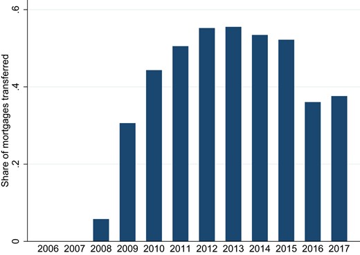
Share of mortgages transferred. This figure shows the share of mortgages transferred over total mortgages from 2008q4 until 2017. Note that although banks started to transfer mortgages from 2007q3 onward, ORBOF provides data on transfers from 2008q4 onward only. Source: ORBOF, with authors’ own calculations.
The birth of the covered bond market was associated with a swap agreement allowing banks to exchange covered bonds for Treasury bills that was launched by the Ministry of Finance in October 2008. Although the Norwegian economy and financial system in general were relatively unaffected by the financial crisis and the Norwegian financial sector did not experience substantial losses (Kragh-Sørensen and Solheim 2014), as a precautionary measure, the Ministry of Finance initiated an arrangement in which the government gave banks treasury bills in exchange for covered bonds for an agreed period, so that banks could improve their asset liquidity. Norges Bank administered the arrangement and Treasury bills with a total value of NOK 230 billion were allocated. The swap agreement was terminated in October 2009; afterward, given that their liquidity pressure was eased, banks terminated their swap agreements and sold the covered bonds in the market. See Bakke and Rakkestad (2010) for more details.
Although the swap arrangement was a temporary measure and only lasted for 1 year, it did kickoff the market and covered bond issuance continued to increase substantially. Particularly, as Figure 2 shows, the rapid growth in covered bond issuance after the termination of the swap agreement was largely driven by demand from foreign investors: As of the end of 2019, 55% of covered bonds outstanding are denominated in foreign currencies; among those foreign currency denominated outstanding covered bonds, 89% are denominated in euro and 6% are denominated in US dollar. Given that mortgage loans in Norway are mostly denominated in Norwegian krone while more than half of Norwegian covered bonds outstanding are denominated in foreign currencies, covered bonds issuing banks are exposed to the interest rate risks on the international bond market and exchange risks from the currency mismatch. Therefore, Norwegian covered bond issuers are required by law to hedge against the interest rate risks and exchange risks using swap contracts (Bakke and Rakkestad 2010). After the end of our sample period, covered bond issuance has continued to experience fast growth. As of 2020q3, covered bonds outstanding in Norway amount to 143 billion euros, equivalent to 43% of Norwegian GDP.
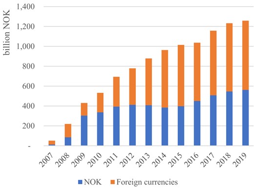
Outstanding debt and currency decomposition of Norwegian covered bonds. This figure shows the outstanding debt (in billion NOK) and currency decomposition (in NOK, denoted by the dark area, or other currencies, denoted by the lighter area) of covered bonds issued in Norway from 2007 until 2019. Source: Norwegian covered bonds statistics, Finance Norway.
3. Data and Methodology
In this section, we outline the data sources we use and describe our empirical approach.
3.1. Data
Our sample period is 2003–2012. Our data is merged from three different data sources. The first data source is quarterly balance sheet data used for supervisory purposes for all Norwegian banks (Statistisk Sentralbyrå 2017). We exclude foreign branches or subsidiaries in Norway and consider only banks issuing mortgages. We drop banks that only existed before the introduction of covered bonds and include new banks from their third quarter of existence onward.9 The data source covers 133 banks and 5,150 bank-quarter observations. It provides us with the volume of mortgage transfers from banks to mortgage companies from 2008q4 onward.
There are 21 mortgage companies in our sample, 11 are owned by one bank and 10 are co-owned by multiple banks.10 In total, 11 banks are not linked to any mortgage company. We consolidate balance sheet items of mortgage companies and banks. If multiple banks share a mortgage company, we consolidate on the basis of the share of mortgages stemming from bank i on the mortgage company’s balance sheet. Between 2008 and 2012, banks transferred on average 15.17% of mortgages to mortgage companies. In aggregate, 30.5% of all mortgages issued were transferred (see Figure 1). We have information on the share of loans on the banks’ balance sheets at LTV ratios above or below 80% in 2006q4.11 This will be important for constructing our treatment indicator, as highlighted in Section 3.2. Table 1 reports summary statistics at the bank-time level.
Summary statistics at the bank level.
| N | Mean | Sd | Min | Median | Max | |
|---|---|---|---|---|---|---|
| Logs | ||||||
| Total assets | 5,150 | 14.957 | 1.409 | 11.934 | 14.674 | 21.519 |
| Total loans | 5,150 | 14.781 | 1.340 | 11.436 | 14.508 | 20.820 |
| Mortgage loans total | 5,150 | 14.506 | 6.226 | 10.087 | 14.302 | 20.283 |
| Mortgage loans transferred to credit company, 2008–2012 | 2,122 | 10.347 | 5.578 | 0.000 | 12.447 | 20.114 |
| Firm loans | 5,138 | 13.358 | 1.562 | 9.680 | 13.018 | 19.667 |
| Securities | 5,150 | 12.404 | 1.677 | 5.628 | 12.164 | 20.113 |
| Ratios | ||||||
| Mortgage loans over total assets | 5,150 | 0.654 | 0.123 | 0.044 | 0.676 | 0.954 |
| Mortgage loans over total loans | 5,150 | 0.773 | 0.128 | 0.051 | 0.793 | 1.000 |
| Firm loans over total assets | 5,138 | 0.219 | 0.083 | 0.010 | 0.209 | 0.810 |
| Firm loans over total loans | 5,138 | 0.261 | 0.101 | 0.010 | 0.251 | 0.935 |
| Securities over total assets | 5,150 | 0.089 | 0.045 | 0.000 | 0.079 | 0.374 |
| Net liquidity over total assets | 5,135 | 0.053 | 0.078 | −0.553 | 0.056 | 0.386 |
| Balance sheet liquidity over total assets | 5,150 | −0.324 | 0.074 | −0.648 | −0.324 | −0.046 |
| Interest income | ||||||
| Mean interest on firm lending in %, yearly | 1,006 | 5.890 | 0.699 | 3.140 | 5.909 | 7.720 |
| Ratio interest firm over interest other lending, yearly | 1,006 | 1.269 | 0.221 | 0.545 | 1.250 | 2.130 |
| Funding costs | ||||||
| Interest paid on total funding in %, yearly | 1,251 | 2.723 | 1.049 | 0.57 | 2.399 | 6.307 |
| Interest paid on subordinated funding in %, yearly | 421 | 8.178 | 5.149 | 0.398 | 6.947 | 46.057 |
| Profitability | ||||||
| Net interest margin, yearly | 1,251 | 0.020 | 0.006 | 0.001 | 0.020 | 0.040 |
Notes: This table reports summary statistics for 133 banks, or 5,150 bank-quarter-year observations. We follow Deep and Schaefer (2004) and define net liquidity over total assets as the share of net liquid assets over total assets as (marked-to-market (MM) assets + central bank reserves − interbank borrowings − certificates)/total assets. We define balance sheet liquidity over total assets as the negative of Berger and Bouwman (2009)’s definition of liquidity creation. We use Berger and Bouwman (2009)’s definition and adapt it to the availability of our balance sheet data. Illiquid assets encompass firm loans, intangible hold-to-maturity (HTM) assets, HTM owner assets and other assets. Liquid assets are assets at the central bank, HTM bonds, other HTM assets, and MM assets. Illiquid liabilites are subordinated debt and equity. Liquid liabilities are deposits and deposits from the central bank. We add the sum of illiquid assets and the sum of liquid liabilities with weights of 0.5 and subtract the sum of liquid assets and illiquid liabilities with weights of 0.5. We divide by total consolidated assets and multiply the index by −1. We estimate the interest on total funding costs in % as the share of interest costs over total liabilities, and the interest on subordinated funding in % as interest costs on subordinated funding over total subordinated debt. We truncate interest paid on subordinated debt at the 1st and the 99th percentile per year due to outliers and set negative values to missings.12
Our second data source is loan level data obtained from the Norwegian Tax Administration (Skatteetaten 2017). By the end of each year, all banks report all outstanding loan and deposit accounts to the tax administration for tax purposes. In total, we observe 3,885,845 firm-account-bank-year observations, based on 250,545 limited liability firms.13 We aggregate loans and deposits to the firm–bank-year level, which results in 1,627,319 firm–bank-year observations. In our dynamic regression estimation we use 1,355,289 firm–bank-year observations for which we can estimate the symmetric growth rate of loans (see below) from 220,059 firms. On average, a firm maintains a relationship to 1.19 banks, and 83.74% of firm-year observations are linked to one bank only. A firm has on average 1.57 loans with its bank conditional on the existence of a loan relationship. Table 2 reports summary statistics at the firm–bank-year level.
Summary statistics at firm–bank-year level.
| N | Mean | Sd | Min | Median | Max | |
|---|---|---|---|---|---|---|
| Log(loans) | 1,355,289 | 4.552 | 6.567 | 0.000 | 0.000 | 23.363 |
| Number of loans per borrower|$|_{\text{loan}\gt 0}$| | 457,962 | 1.566 | 1.950 | 1.000 | 1.000 | 310.000 |
| Symmetric credit growth (|$\Delta L_{b,f,t}$|) | 1,355,289 | −0.067 | 0.710 | −2.000 | 0.000 | 2.000 |
| Interest rate (|$i_{b,f,t}$|, in %) | 401,673 | 6.614 | 3.595 | 0.000 | 6.166 | 35.473 |
Notes: This table reports summary statistics for 275,323 firm–bank relationships, or 220,059 firms.
In the loan level regressions we use the symmetric growth rate of credit as dependent variable, defined as
where |$D_{b,f,t}$| is the outstanding credit volume between bank b and firm f in year t.
We use the fact that we observe both the outstanding debt volume and the interest paid to compute a proxy for the interest rate for every firm–bank-year combination. This interest rate proxy is defined as
We only include interest payments if we also observe a loan in year |$t-1$|. To limit the influence of outliers, we truncate |$i_{b,f,t}$| at the 1st and the 99th percentile.
Our third and final data source is firm-level data from a major credit rating agency on all major balance sheet items and other information on the universe of Norwegian limited liability firms (Bisnode 2017). We add information on firm age, rating, and balance sheet variables to investigate the role of firm characteristics in explaining banks’ potential change in credit allocation following the introduction of covered bonds. We exclude financial firms. Table 3 shows summary statistics. We merge 130,661 firms (933,746 firm-year observations). The median firm has total assets of approximately NOK 2,782,000,14 is 10 years old and has an A rating.15 We define a binary variable |${Rating}(0/1)$| which is 0 for low-rated firms (A, B, or C) and 1 for high-rated firms (AA or AAA).
Summary statistics at firm-year level.
| N | Mean | Sd | Min | p50 | Max | |
|---|---|---|---|---|---|---|
| Size and Age | ||||||
| Assets (in 1000s of NOK) | 933,746 | 42,270.250 | 1,563,833 | 0.000 | 2,782.000 | |$5.84\times 10^8$| |
| Age | 933,738 | 13.71379 | 13.00164 | 0.000 | 10.000 | 169.000 |
| Rating | ||||||
| Rating (AAA:5 - C:1) | 933,746 | 3.278 | 0.991 | 1.000 | 3.000 | 5.000 |
| Rating(0/1) | 933,746 | 0.425 | 0.494 | 0.000 | 0.000 | 1.000 |
Notes: This table reports summary statistics for 130,661 firms.
3.2. Empirical Strategy
3.2.1. Endogenous Regressions
To assess whether banks change their portfolio composition when issuing covered bonds, an initial, naive approach would be to regress outcome variables such as mortgage lending on covered bond issuance. In such a case, however, reverse causality or omitted variable bias would be a potential issue and, as such, the coefficient should not be interpreted as causal. In Table 4, we show results for such an endogenous regression. We use log-level balance sheet positions as dependent variables and the share of mortgages transferred to cover pools as right-hand side variable. We observe that a higher share of mortgages transferred (|${transfers}_{t-1}$|) goes along with increased size of the balance sheet (column I), and an increased loan portfolio (column II). We find a mild positive correlation with mortgages (column III) and a strong positive correlation with firm loans (column IV). Also, securities holdings is positively correlated with transfers (column V). However, to the extent that mortgage lending affect banks’ ability to transfer loans to the cover pool, we likely overestimate the effect of covered bond issuance in particular on mortgage lending. For this reason, we develop the identification approach outlined below.
Endogenous regressions.
| (I) | (II) | (III) | (IV) | (V) | |
|---|---|---|---|---|---|
| Total assets | Total loans | Mortgages | Firm loans | Securities | |
| Transfers|$_{t-1}$| | 0.260*** | 0.151** | 0.131* | 0.323*** | 0.663*** |
| (0.068) | (0.070) | (0.067) | (0.103) | (0.206) | |
| Observations | 2,122 | 2,122 | 2,122 | 2,122 | 2,122 |
| R-squared | 0.588 | 0.561 | 0.561 | 0.253 | 0.250 |
| Number of banks | 130 | 130 | 130 | 130 | 130 |
| Bank FE | Yes | Yes | Yes | Yes | Yes |
| Year FE | Yes | Yes | Yes | Yes | Yes |
In this table, we show results from estimating the following regression: |$Y_{b, t} = \alpha _b + \alpha _T + \beta \: {Transfers}_{(t-1)} + \epsilon _{b,t}$|. |$Y_{b,t}$| are logs of total assets, total loans, mortgages, firm loans, and securities. |${Transfers}_{(t-1)}$| is the share of total mortgages which banks transfer to cover pools in the previous quarter. The regression covers the time period 2008q4–2012q4 due to data availability of transfers, and includes year FEs |$\alpha _T$|. Robust standard errors are clustered at the bank level and are depicted in parentheses. *, **, and *** indicate significant coefficients at the 10%, 5%, and 1% level, respectively.
3.2.2. Cross-sectional Variation in Covered Bond Exposure
Our empirical strategy exploits the fact that only mortgages with an LTV below 75% (“low LTVs”) were eligible for being transferred to the cover pool. As a result, banks with different initial distributions of LTVs in their mortgage portfolios had different scope for issuing covered bonds. As described in Section 3.1, we observe the breakdown of the volume of mortgages with an LTV below and above 80%. We use this information to approximate the fraction of loans for each bank below the regulatory threshold of 75%. We construct a treatment indicator equal to 1 for banks that had a share of low LTV mortgages over total mortgages that is above the median of all banks in the quarter before the covered bond introduction (2006q4), that is, |$T_b =1$|. We set |$T_b =0$| for all other banks and refer to them as “low-exposure banks” or “other banks” throughout the text.16 On average, 84.2% of mortgages on banks’ balance sheets have low LTVs. Banks that we define as high-exposure had on average 89.2% low LTV mortgages, while other banks had on average 79.2% low LTV mortgages in 2006q4. In line with Callaway, Goodman-Bacon, and Sant’Anna (2024), we also use the continuous ratio of low LTV mortgages over total mortgages as the treatment measure in a robustness exercise and show that the results remain qualitatively similar. Table 5 shows summary statistics on our treatment indicators.
Summary statistics on treatment definitions.
| N | Mean | Sd | Min | Median | Max | |
|---|---|---|---|---|---|---|
| |$T_b$| (treatment indicator at bank level) | 5,150 | 0.496 | 0.500 | 0.000 | 0.000 | 1.000 |
| Share of mortgages transferred to mortgage companies, 2007–2012 | 3,048 | 0.106 | 0.140 | 0.000 | 0.038 | 0.869 |
| Ratio of low LTV mortgages over total mortgages, 2006q4 | 133 | 0.842 | 0.064 | 0.662 | 0.850 | 1.000 |
| Ratio of low LTV mortgages over total mortgages, 2006q4, |$T_b = 1$| | 67 | 0.892 | 0.039 | 0.850 | 0.876 | 1.000 |
| Ratio of low LTV mortgages over total mortgages, 2006q4, |$T_b = 0$| | 66 | 0.792 | 0.039 | 0.662 | 0.799 | 0.844 |
| |$T_b$| (treatment indicator at loan level) | 1,355,289 | 0.880 | 0.325 | 0.000 | 1.000 | 1.000 |
Notes: This table reports summary statistics on variables used for the treatment definition for 133 banks, or 5,150 bank-quarter-year and for 275,323 firm–bank links.
Note that our treatment definition does not exclude the possibility that low-exposure banks issue covered bonds. We merely capture the fact that high-exposure banks could more readily issue covered bonds due to the availability of eligible mortgages on their balance sheets. Hence, we capture the difference in the intensity of exposure to the introduction in covered bonds. To illustrate this difference, we show in Figure 3 the fraction of mortgages transferred to the cover pools for high-exposure banks and other banks, respectively. By 2011, the fraction of mortgages transferred by high-exposure banks was approximately 70% larger compared with other banks.17
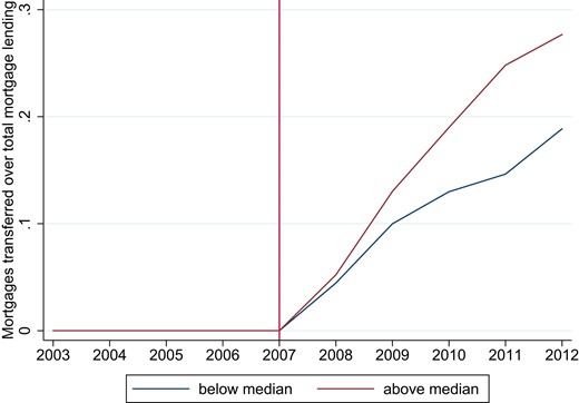
Share of mortgages transferred for high-exposure and low-exposure banks. This figure shows the average share of mortgages transferred to credit companies over total mortgages issued by high-exposure banks in red (upper line), and other banks in blue (lower line). We define high exposed banks as having a share of low-LTV mortgages over total mortgages that is above the median of all banks before the covered bond introduction in 2006q4.
Over time, other banks can shift the supply of credit toward low-LTV mortgages relative to high-exposure banks. However, this is likely to be a slow-moving process, as shown in Figure C.1 in Online Appendix C, as the cross-sectional differences in the average LTV in banks’ mortgage portfolios not only reflect bank factors, but also relatively persistent regional factors such as house prices and borrower type heterogeneity more broadly. However, over time it is likely that banks can adjust the composition of mortgage credit to improve the scope for issuing covered bonds. Hence, our treatment measure |$T_b$| is meant to capture the short- and medium-run effects of exposure to the introduction of covered bonds. We therefore focus on the impact of covered bonds on bank outcomes only up until 6 years after the legal change was implemented.
At the bank level, the fraction of low-LTV mortgages has strong predictive power on post-treatment mortgage transfers to cover pools. In Table 6, we report the results from a univariate regression of the fraction of mortgages transferred post-treatment against the pre-treatment fraction of low-LTV mortgages. There is a strong and statistically significant relationship, suggesting that a 1 percentage point increase in the ratio of low-LTV mortgages to total mortgages pre-treatment is associated with a 0.19 percentage point increase in the fraction of transferred mortgages post-treatment. Moreover, the fraction of low-LTV mortgages explains roughly half of the variation in the fraction of mortgages transferred. We thus conclude that our exposure measure captures banks’ subsequent issuance of covered bonds well.
Share of eligible mortgages predict mortgage transfers.
| Mortgage transfers over total mortgages | |
|---|---|
| Eligible mortgages over total mortgages | 0.190** |
| (0.089) | |
| Observations | 5,150 |
| Number of banks | 133 |
| R-squared | 0.484 |
| Mortgage transfers over total mortgages | |
|---|---|
| Eligible mortgages over total mortgages | 0.190** |
| (0.089) | |
| Observations | 5,150 |
| Number of banks | 133 |
| R-squared | 0.484 |
Notes: This table shows the correlation of the share of eligible mortgages over total mortgages in 2006q4 and the actual share of mortgages transferred to mortgage companies over total mortgages issued. The regression includes quarter-year FEs. *, **, and *** indicate significant coefficients at the 10%, 5%, and 1% level, respectively.
In Table B.1 in Online Appendix B, we report summary statistics on a range of outcomes for banks defined as high-exposure and other banks in the pre-reform period. We also include the results from t-tests on the difference between the two groups. Importantly, our identification strategy outlined below does not rely on similarities in these measures across high- and low-exposure banks. High-exposure banks are larger in size and issue slightly more mortgages and firm loans. The share of loans over total assets is slightly lower for the high-exposure banks, though the difference amounts to 0.007 percentage point only. The two groups do not differ in terms of mortgages and firm loans over total assets or over total loans. High-exposure banks hold less securities (HTM financial assets plus MM financial assets) over total assets compared with other banks. The difference is with 0.3 percentage points small, but statistically significantly different from zero. We include bank FEs in our regression specification in order to control for level differences. In the robustness check in Section 4.4, we further show that banks do not differ in terms of ex ante risk-taking behavior. Further, we provide evidence that results remain robust when we exclude the ten largest banks from the sample.
In the next subsections, we outline our empirical strategy at the different levels of analysis.
3.2.3. Bank Level
We estimate the following dynamic estimation equation at the bank level:
Dependent variables |$Y_{b,t}$| are balance sheet items of bank b in year-quarter t. We focus on outcomes in log levels and ratios. The regression includes bank FEs (|$\alpha _b$|) and quarter-year FEs (|$\delta _\tau$|). Standard errors are clustered at the bank level.
We interact the treatment variable |$T_b$| with indicators for every quarter-year. We leave out 2006q4 as the base quarter-year before the introduction of covered bonds in 2007. With this dynamic approach, we can trace the effect of the issuance of covered bonds on a quarterly basis. Moreover, we can investigate whether outcomes differ pre-treatment by testing whether |$\gamma _{\tau }$| is significantly different from zero for |$\tau \lt 2006q4$|.
3.2.4. Loan Level
We estimate the following dynamic estimation equation at the firm–bank level:
Dependent variables are symmetric growth of loans of firm f with bank b in year t defined as in equation (1), as well as the interest rate paid by firm f to bank b in year t, approximated as in equation (2). We interact the treatment variable |$T_b$| with indicators for every year. We leave out 2006 as the base year before the introduction of covered bonds in 2007. We include bank–firm FEs |$\alpha _{f,b}$|, as well as time FEs (|$\delta _\tau$|), and cluster standard errors at the bank level.
To control for firm-level demand shocks, we exploit the structure of our loan level data to control for different firm characteristics to ensure that we compare outcomes from relatively similar firms. Specifically, we follow two different approaches. First, we follow Degryse et al. (2019) and introduce industry-location-size-time FEs, defined as the two-digit industry code, two-digit zip-code, deciles of total assets, and year to control for local, industry-specific, and size-specific demand effects. Their approach is especially suitable for data consisting of many small firms with single bank links, as in our case (83.74% of firm-year observations are by firms linked to one bank only). Second, we follow Khwaja and Mian (2008) and introduce firm-time FEs in the sample of multi-bank firms.
3.3. Threats to Identification
Our identifying assumption is that the outcomes we consider would be similar—conditional on a set of FEs depending on the level of analysis—for high- and low-exposure banks in the absence of the introduction of covered bonds. Conditional on this assumption being true, we can then interpret our estimates as the causal effect of covered bond issuance on bank outcomes in the short- and medium-run. In this section, we discuss factors which may potentially invalidate this interpretation. It is useful to group the potential identification challenges into four: systematic differences, confounding credit demand shocks, confounding credit supply shocks, and anticipation effects.
3.3.1. Systematic Differences
The first threat to identification is that banks with different initial mortgage portfolios are structurally different in terms of outcomes. For instance, if banks with a high fraction of low LTV mortgages and thus a larger share of cover pool transfers increase their firm lending share throughout our sample period, we would estimate a positive and significant effect of low-LTV mortgages on firm lending that would not be due to the introduction of covered bonds.
An advantage in our dynamic difference-in-differences approach is that it allows us to directly test for systematic differences between banks according to the exposure measure, by estimating period-specific treatment effects also prior to the introduction of covered bonds. Specifically, we can explore if there were parallel trends among banks with different fractions of low-LTV mortgages prior to the transition by testing if |$\gamma _{\tau }=0 \forall \tau \lt 2006q4$| in equations (3) and (4).
3.3.2. Confounding Credit Demand Shocks
Even if banks with different exposures to the introduction of covered bonds are similar prior to 2007, they may experience different credit demand shocks in the subsequent years. This is a concern as the introduction of covered bonds coincided with the financial crisis, which could affect firms differently. Shocks to banks’ firm clients could affect our results if firms and banks are systematically linked. For instance, banks that are less exposed to the introduction of covered bonds could lend more to export-oriented firms, or more generally to regions with relatively high exposure to the international downturn associated with the financial crisis. In that case, differences in credit growth between banks with different initial fractions of low-LTV mortgages could be a result of a reduction in credit demand from customers of low-exposed banks rather than an increase in credit supply by high-exposed banks.
In order to alleviate this concern, we control for firm demand shocks with an extensive set of FEs, that is, industry-location-time-size FEs as well as firm-time FEs as described in Section 3.2.4. The latter approach holds firm factors fixed, provided that they are invariant at the firm |$\times$| year level. Moreover, by observing both quantities and prices at the loan level, we can exploit the fact that demand and supply shocks move prices in opposite directions. For instance, an increase in the volume of credit and a decline in the interest rate on loans from high-exposure banks would only be consistent with a relative expansion in the supply of credit.
3.3.3. Confounding Supply Shocks
A third threat to identification could arise if there are other factors affecting banks’ supply of credit that are correlated with our exposure measure. One potential concern is that banks with a large fraction of low-LTV mortgages were less exposed to the financial crisis and as a result had higher risk-bearing capacity than other banks, which in turn could induce them to rebalance their portfolio.
In general, the Norwegian economy and financial system were relatively unaffected by the financial crisis. Norwegian banks were affected indirectly in primarily two ways. First, banks to varying degrees invested in financial assets that would potentially depreciate in value ex post due to the ongoing crisis. This would especially be a relevant concern for financial instruments that are MM. Second, a more indirect contagion happened in the form of short-term liquidity stress in Norwegian interbank markets. The interbank spread increased substantially in mid-September 2008. It was lowered to pre-crisis level toward the end of 2008, but in theory this short-term disruption in access to liquidity could confound at least some of our results.
In order to gauge the severity of these concerns, we investigate how our treatment measure correlates with (1) banks’ holdings of financial instruments that are MM and (2) banks’ reliance on interbank funding, both measured at the end of 2006. A negative correlation between our treatment measure and these measures would indicate that exposure to the crisis through either measure could pose an identification concern.
Further, changes in risk-taking behavior during the financial crisis conditional on our treatment measure might confound our results. If low-exposed banks had a larger risk appetite before the financial crisis and became more risk averse during the crisis as in Guiso, Sapienza, and Zingales (2018), differential effects between high-exposure and other banks might be merely driven by relative changes in risk aversion over time. In order to address this concern, we investigate differences in ex ante risk-taking across high- and low-exposure banks using a wide range of proxies for risk-taking, including volatility of earnings, net liquidity, and equity ratios, and use all proxies as controls in our estimations.
Additionally, high exposure banks are larger banks, which might have been differently affected by the financial crisis compared to smaller banks. For example, larger banks might had a greater need to diversify during the financial crisis and hence increased supply of firm loans relative to smaller banks.18 We employ bank FEs to control for static differences in all regressions, as well as exclude the three, five, and ten largest banks from our sample in robustness checks to rule out that our results are driven by different exposure to the financial crisis due to size differentials.
A final potential confounding credit supply shock is the transition to Basel II. The transition to Basel II took place in 2007, and entailed for most banks a reduction in average risk-weights, applied to retail loans and mortgages with a low LTV. This could then imply that there was also a larger reduction in the effective capital requirement for banks that were high-exposure according to our measure and that this relative reduction in the capital requirement is driving our results. The largest absolute reduction in risk weights for banks computing risk weights under the standard method was for retail firm loans.19 As a robustness check, we therefore use balance sheet information and actual changes in risk weights to compute—bank by bank—the actual reduction in the capital requirement due to the Basel II transition. We can then correlate the capital requirement reduction with our treatment measure to investigate whether banks that were more exposed to the Basel II transition were also more exposed to the introduction of covered bonds.
3.3.4. Anticipation Effects
A final concern is that high-exposure banks according to our measures adjusted prior to the introduction of covered bonds. This is a valid concern if the introduction of covered bonds were known well in advance. Note that such anticipation effects are likely to lead us to underestimate the effects of covered bond issuance. Judging from Figure C.1 in Online Appendix C, it seems unlikely that banks selected themselves into the group of high-exposed banks, as the share of eligible mortgages in the pre period is fairly stable over time. Moreover, the flexible difference-in-differences approach allows us to explicitly map out when high-exposure banks adjust relative to the actual introduction of covered bonds and hence we can be somewhat agnostic about the exact timing of the treatment.
4. Results
In this section, we assess the impact of covered bond issuance on banks’ balance sheets. We also outline a theoretical model to explain how covered bond issuance affects bank portfolio allocation and test the model’s predictions. We end the section by showing a series of robustness exercises.
4.1. Results on Portfolio Rebalancing
4.1.1. Bank Level (levels)
We start by comparing the evolution of different asset classes at the bank level. We show results of differences across log level of total assets, as well as mortgage and firm loans in Figure 4, with corresponding statistics in Table 7.

Regression information corresponding to Figure 4.
| Dependent variable | Figure | N observations | N cluster | R2 | Mean dependent | SD dependent |
|---|---|---|---|---|---|---|
| Total assets | 4a | 5,150 | 133 | 0.882 | 14.957 | 1.409 |
| Mortgages | 4b | 5,150 | 133 | 0.867 | 14.506 | 1.340 |
| Firm loans | 4c | 5,138 | 133 | 0.679 | 13.358 | 1.562 |
Notes: This table reports statistics from estimating equation (3). The second column (“Figure”) refers to the corresponding coefficient plot.
First, consider how the introduction of covered bonds has affected total balance sheet size in Panel 4a. High exposure banks increase their balance sheets after the introduction of covered bonds in comparison to low exposure banks, measured according to the log of total assets. The difference is significantly different from zero after the introduction of covered bond markets up to the 1% level in 2011q4. Next, consider how the introduction of covered bonds has affected mortgage lending in Panel 4b. We do not find a difference in mortgage lending, measured according to the log of mortgages on banks’ balance sheets, between high exposure and low exposure banks. This lack of response is inconsistent with the view that covered bonds would lead to an expansion of mortgages as often discussed (Nicolaisen 2017). In contrast, however, we show that firm lending—in Panel 4c, increases for high exposure banks in comparison to low exposure banks after the introduction of covered bond markets suggesting that the exposure to covered bonds contributes to a relative shift of credit toward firm lending. The difference between high exposure and low exposure banks is statistically significantly different from zero up to the 1% level in 2008q4 and 2011q4. The results reflect findings from the endogenous regressions presented in Table 4. As argued, in the latter approach, we likely overestimate the relationship between covered bond issuance and outcome variables such as lending decisions. In contrast, with our estimation strategy, we find that as a response to the introduction of covered bond markets, banks do not change their mortgage lending, but increase firm lending.
Note that we observe differential effects in a period of overall loan growth. See Figure C.2 in Online Appendix C for the evolution of the mean stock of loans on banks’ balance sheets. Online Appendix Figure C.2 suggests that both, high- and low-exposure banks increase lending over time, though high exposure banks increase firm lending more than low exposure banks.
4.1.2. Bank Level (Portfolio Shares)
To further illustrate how covered bonds leads to a portfolio rebalancing toward firm lending, we continue by presenting results for portfolio rebalancing in ratios, that is, the proportions of the lending portfolio that go into mortgage lending or firm lending. We present the results in Figures 5 and 6. Accompanying statistics of the regression output are listed below in Table 8. Note that results hold also for the continuous treatment definition instead of the binary definition.20
Bank portfolio re-balancing: total lending and mortgage lending. In this figure, we show the average loan and the average mortgage share over time on the left hand side. On the right hand side, we show the coefficient plots with confidence intervals at 90% from estimating equation (3). Statistics from estimations can be found in Table 8.
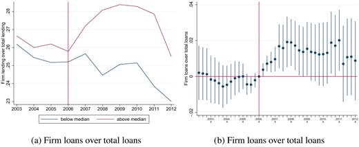
Bank lending portfolio re-balancing: firm lending. In this figure, we show the average firm share over time on the left hand side. On the right hand side, we show the coefficient plots with confidence intervals at 90% from estimating equation (3). Statistics from estimations can be found in Table 8.
| Dependent variable | Figure | N | No. of banks | R2 | Mean of dep. var. | Sd of dep. var. |
|---|---|---|---|---|---|---|
| Mortgage loans over total loans | 5b | 5,150 | 133 | 0.260 | 0.773 | 0.128 |
| Firm loans over total loans | 6b | 5,138 | 133 | 0.054 | 0.261 | 0.101 |
| Dependent variable | Figure | N | No. of banks | R2 | Mean of dep. var. | Sd of dep. var. |
|---|---|---|---|---|---|---|
| Mortgage loans over total loans | 5b | 5,150 | 133 | 0.260 | 0.773 | 0.128 |
| Firm loans over total loans | 6b | 5,138 | 133 | 0.054 | 0.261 | 0.101 |
Notes: This table reports statistics from estimating equation (3). The second column (“Figure”) refers to the corresponding coefficient plot.
| Dependent variable | Figure | N | No. of banks | R2 | Mean of dep. var. | Sd of dep. var. |
|---|---|---|---|---|---|---|
| Mortgage loans over total loans | 5b | 5,150 | 133 | 0.260 | 0.773 | 0.128 |
| Firm loans over total loans | 6b | 5,138 | 133 | 0.054 | 0.261 | 0.101 |
| Dependent variable | Figure | N | No. of banks | R2 | Mean of dep. var. | Sd of dep. var. |
|---|---|---|---|---|---|---|
| Mortgage loans over total loans | 5b | 5,150 | 133 | 0.260 | 0.773 | 0.128 |
| Firm loans over total loans | 6b | 5,138 | 133 | 0.054 | 0.261 | 0.101 |
Notes: This table reports statistics from estimating equation (3). The second column (“Figure”) refers to the corresponding coefficient plot.
First, consider how the introduction of covered bonds affected the share of mortgage lending in total lending of banks. Figure 5a plots the raw data of the share of mortgage lending over total loans. There is a divergence in mortgage lending between the two groups from 2008 and onward, where the high-exposure banks have a relative decrease in the share of mortgages. Importantly, given that the data is consolidated at the bank-credit company level, this reduction in the fraction of mortgages is not mechanically related to mortgages being transferred to the mortgage company for the purpose of issuing covered bonds but rather reflects the fact that mortgage lending is unchanged while overall loans—due to the increase in firm lending—increases as documented in the previous section. In Figure 5b, we plot the coefficients from estimating equation (3) with mortgages over total loans as dependent variable. Before the introduction of covered bonds, there are no statistically significant time-varying differences between the two groups. After the introduction, high-exposure banks lower their mortgages to total loans ratio compared with other banks. The differences are statistically significantly different from zero at the 5% level from 2008q2 and at the 1% level from 2008q4 onward. The relative reduction in the mortgage share is driven by a relative increase in total lending due to the increase in firm lending, whereas total mortgage lending does not differ between the two groups, as we show in Figure 4. The reduction in the mortgage share is quantitatively large. High-exposure banks lowered the mortgage share by up to 5.7 percentage points compared with other banks over the post period. This compares to a pre-period mortgage share for high-exposure banks of 74.3%, suggesting that the relative reduction in the mortgage share in the post period is sizable and corresponds to around 7.7% of the average mortgage share of high-exposure banks in the pre period.
Next, we assess the fraction of firm loans relative to total loans. In Figure 6a, we illustrate that firm loans increase for high-exposure banks relative to other banks post-2007. In Figure 6b, we show that there are no differences between the two groups in the pre period compared with 2006q4. Differences in the post period are statistically significantly different from zero at the 1% level in 2007q2 and at the 5% level thereafter until 2009q2, with varying significance levels afterward. The firm lending share is up to 1.9 percentage points higher for high-exposure banks compared with other banks. This is an increase of 7.5% relative to the average share of firm lending for high-exposure banks in the pre period (25.7%). In terms of timing, effects as shown as in Figure 6b are particularly strong 2007–2009, when the growth rate of issuance of covered bonds was particularly strong (see Figure 2).
A valid concern against our identification could be that it is not the high-exposed banks which adjust their lending portfolios, but low-exposed banks which actually increase their mortgage lending in order to be able to participate in covered bond markets and hence we see a negative differential effect between high and low exposed banks in terms of the share of mortgages in their lending portfolio. However, there are two stylized facts which speak against this hypothesis: First, as we show in Figure 6a, there is a clear surge in the share of firm loans over total loans for high exposed banks after the introduction of covered bond markets. Second, there is actually no difference in mortgage lending between the two groups, as we show in Figure 4b, where we compare log level mortgage issuance. The difference between the two groups is driven by increases in firm lending by high exposed banks compared to low exposed banks (see Figure 4c).
4.1.3. Loan Level
Next, we turn to the loan level to further shed light on the increase in firm lending. Using loan level data, we can tighten identification by adopting firm controls to address possible confounding firm-level demand shocks. We estimate the dynamic regression equation (4) with the symmetric growth rate of debt as defined in equation (1) and our interest proxy as defined in equation (2) as dependent variables. Further, we provide evidence for whether the increase in firm credit for high-exposure banks is uniform across all firms, or whether it is driven by a subset.
Loan growth and interest rates. In Figure 7a, we show the average of the symmetric growth rate of loans extended by high-exposure banks in red, and for loans extended by other banks in blue over time. After the introduction of covered bonds, loan growth for loans stemming from high-exposure banks increases, whereas loan growth decreases for loans from other banks. In Figure 7b, we plot the coefficients from estimating equation (4) with symmetric growth of debt as the dependent variable. Estimation results and accompanying statistics are reported in Table B.2 in Online Appendix B. Loan growth does not differ in the pre-reform period between the two groups. From 2008 onward, loan growth from high-exposure banks is larger than from other banks compared with base year 2006. The difference is statistically significantly different from zero at the 1% level for most years. High-exposure firm–bank pairs have a symmetric growth rate which is on average up to 0.05 higher than for other firm–bank pairs. The relative change is substantial: it compares to an average symmetric growth rate for loans from high-exposure banks in the pre-reform period of −0.073. These results are consistent with the findings at the bank level.21
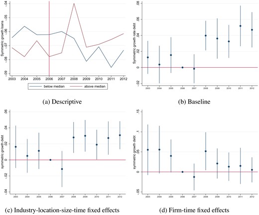
Changes on loan growth on the loan level. In Figure 7a, we show mean symmetric loan growth for loans with high-exposure banks ("above median") and loans with other banks ("below median") over time. In Figure 7b, we show coefficient plots from estimating the dynamic regression equation (4) with confidence intervals at 90% with symmetric growth for loans as dependent variable. In Figure 7c, we include industry-location-time FEs, and in Figure 7d, firm-time FEs. In Table B.2 in Online Appendix B, columns I–III show the results.
To further sharpen identification, we apply the estimation strategy as proposed by Degryse et al. (2019) and introduce industry-location-size-time FEs to control for confounding loan demand shocks. In Figure 7c, we show the corresponding coefficient plot. Again, we do not observe differences between the two groups in the pre-reform period. From 2008 onward, loans from high-exposure firm–bank pairs have larger loan growth than loans from other banks. The difference is statistically significantly different from zero in 2010 at the 10% level, in the years 2008, 2009, and 2011 at the 5% level and in the year 2012 at the 1% level. The symmetric growth rate for loans from high-exposure banks is up to 0.031 higher than the symmetric growth rate for loans from other banks. Given that the average symmetric growth rate for high-exposure firm–bank pairs in the pre-reform period is −0.048, we observe again a substantial relative increase.
Finally we follow Khwaja and Mian (2008) and introduce firm–year FEs for the sample of firms borrowing from multiple banks. In Figure 7d, we show the corresponding coefficient plot. There are no differences between the two groups in the pre period. Although our estimates become more imprecise, we still observe a positive difference between the two groups for the post-treatment year 2008, which is statistically significantly different from zero at the 10% level. In terms of economic magnitude, loan growth increases by 0.052 for high-exposure firm–bank pairs compared with loan growth for other firm–bank pairs, which compares to the average symmetric growth rate in the pre-reform period for high-exposure firm–bank pairs in this sub-sample of −0.059.
Part of the reason why the Khwaja–Mian approach yields weak results, is that the sample of multi-bank firms are relatively unaffected by the introduction of covered bonds. To further explore this, we split our sample into firms with a single bank link and multiple bank links, and re-estimating equation (4) for both groups excluding firm–year FEs. We present results in Figure B.1 in Online Appendix B. We observe a significant positive effect on the credit growth of firms with a single bank relationship, indicated in blue, whereas credit growth is only higher in 2008 for firms with multiple bank relationships, shown in red. The overall effect on loan growth is therefore primarily driven by single bank firms, which are not part of the sample in the setting by Khwaja and Mian (2008). We conclude that the approach by Khwaja and Mian (2008) is therefore confining us to a subsample for which the effects of covered bonds issuance is relatively weak.
To investigate whether banks changed their pricing behavior, we next examine the impact of being linked to a high-exposure bank on the proxied interest rate. In Figure 8a, we show the development of interest rates for high-exposure firm–bank pairs and other firm–bank pairs over time. The raw data suggest that firms paid slightly lower interest rates after 2009 if the loan stemmed from a high-exposure bank. In Figure 8b, we show the coefficient estimates from estimating equation (4) with our proxy for the interest rate as dependent variable. We can see a slight move towards lower interest rates for loans from high-exposure banks. The estimates, however, are somewhat imprecise, and we cannot reject the null hypothesis that the coefficients are zero. As before, we follow Degryse et al. (2019) and introduce industry-location-size-time FEs and plot the corresponding coefficients in Figure 8c. Again, we see a negative difference between the two groups in the post-reform period, but the difference is imprecisely measured. Finally, we proceed by introducing firm-time FEs as in Khwaja and Mian (2008). Figure 8d shows the corresponding coefficient plot. The results are in line with the previous findings.
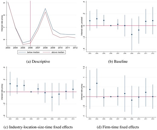
Changes in interest rate proxy at the loan level. In Figure 8a, we show the mean interest rate paid for loans with high-exposure banks ("above median") and with other banks ("below median") over time. In Figure 8b, we show coefficient plots from estimating the dynamic regression equation (4) with confidence intervals at 90% with the interest rate proxy as dependent variable. In Figure 8c, we include industry-location-time FEs, and in Figure 8d firm-time FEs. In Table B.2 in Online Appendix B, columns IV–VI show the results.
Importantly, the results in Figure 8 suggest that interest rates do not increase for loans from high-exposure banks. This, combined with the fact that point estimates decline, provides support for our interpretation of the results above, namely, that the increase in firm credit comes from a credit supply expansion rather than an increase in credit demand.
Low-rated and young firms obtain more lending. Next, we assess whether the increase in firm credit is uniform across all firms or driven by a subset of firms. Two important dimensions for understanding the heterogeneous impact of credit supply expansions in the existing literature are firm risk and firm age (Gertler and Gilchrist 1994; Holmström and Tirole 1997). We therefore group the firms in our sample according to firm rating and firm age in 2006. We define a firm as low-rated if it has a rating of A or below (A, B, or C), and a firm as high-rated if it has a rating of AA or AAA. We define a firm as young if it has an age below or equal to the median firm age (8 years), and a firm as old if it has an age above the median. We re-estimate equation (4) for the sample of low- and high-rated firms, as well as young and old firms separately, using the symmetric growth rate of loans as dependent variable.
In Figure 9, we show coefficient plots and in Table B.4 in Online Appendix B regression results. In Figure 9a, we show that for the sample of low-rated firms there is is a positive differential effect between high-exposure and low-exposure banks from 2008 and onward, which lasts until the end of the sample period and amounts to up to 0.063. For ex ante high-rated firms, there is a significant difference in 2008, which levels off quickly. As we show in Table 9, the symmetric growth rate of debt on average increases by 0.05 for ex ante low-rated firms that borrow from high-exposure banks compared with other banks. Given that the average growth rate for all treated firm–bank pairs in the pre period is −0.073, the differential effect between high- and low-exposure banks of 0.05 is again substantial. For the sample of high-rated firms the average differential effect is close to zero.
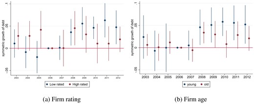
Changes in loan growth at the loan level conditional on firm rating and age. In this figure, we show coefficient plots from estimating the dynamic regression equation (4) with confidence intervals at 90% with symmetric growth for loans as dependent variable. We split the sample according to firm rating or the median firm age in 2006. Low-rated firms had a rating of A, B, or C, and high-rated firms a rating of AA or AAA. Young firms are aged 8 years or below, old firms above 8 years. Table 9 shows the average differential effect in the post period for the two samples, respectively. Table B.4 in Online Appendix B shows the complete regression output.
Summarizing symmetric growth of debt across bank-firms.
| Sample split by... | Low | High |
|---|---|---|
| Rating | 0.050*** (0.012) | 0.000 (0.011) |
| Age | 0.049*** (0.012) | 0.021** (0.008) |
| Sample split by... | Low | High |
|---|---|---|
| Rating | 0.050*** (0.012) | 0.000 (0.011) |
| Age | 0.049*** (0.012) | 0.021** (0.008) |
Notes: This table summarizes the estimated treatment effect from estimating equation (4) splitting the sample according to firm age or firm rating in 2006. Robust standard errors are clustered on the bank level and are depicted in parentheses. *, **, *** indicate significant coefficients at the 10%, 5%, and 1% level, respectively.
In Figure 9b, we show the results when grouping firms according to age. The relative increase in credit is larger for the sample of young firms, consistent with Gertler and Gilchrist (1994).
4.1.4. Liquid Assets at Bank Level
Next, we assess whether there are changes in banks’ investments in financial assets. As in Section 4.1.2, the unit of analysis is now bank |$\times$| year-quarter, and we estimate equation (3) with financial asset holdings as dependent variables.
In Figure 10, we plot the raw data in the left column, and coefficients from a dynamic regressions in the right column. We aggregate HTM financial instruments and MM financial instruments together and call it total security holdings. We assess the ratio of security holdings over total assets. We show the evolution of security holdings over time in Figure 10a. High-exposure banks change their investment behavior into securities after the introduction of covered bonds. Specifically, the share of securities over total assets increases relative to other banks.
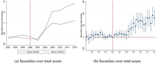
Bank portfolio re-balancing: Financial assets. In this figure, we show the mean dependent variable of the raw data over time in the left column. In the right column, we show the coefficient plot with confidence intervals at 90% from estimating equation (3). Statistics from estimations can be found in Table 10.
In Figure 10b, we show that there are no statistically significant differences between the different bank types before the introduction of covered bonds. In the post period, the difference increases and high-exposure banks have a higher share of securities over total assets compared to other banks. The difference is statistically significantly different from zero at varying levels up to 2010q1 and at the 1% level thereafter. Up to 2012q3, high-exposure banks increase the share of securities by 3.7 percentage points. Given that the share of securities over total assets for high-exposure banks in the pre-reform period period is 7.2%, the relative increase corresponds to around 51.3% of the average share of securities to total assets for high exposed banks in the pre period.
Overall, we conclude that the holdings of securities for the high-exposure banks increase compared to low-exposure.
4.2. Results on Bank Balance Sheet Liquidity, Risk, and Profitability
In the previous section, we documented an increase in lending to risky firms as well as an increase in the holdings of securities which typically have a high degree of market liquidity. An important question is whether the balance sheet adjustments lead to overall riskier banks due to increased credit risk, or whether the increased holdings of liquid financial assets offset credit risk, or even outweigh it. In this section, we therefore investigate how covered bonds impact overall bank risk, taking into account overall balance sheet liquidity, credit risk, and bank profitability.
4.2.1. Liquidity versus Credit Risk
Covered bonds can increase banks’ funding liquidity as covered bonds are a source of long-term funding, as well as market liquidity as banks can invest the proceeds in liquid assets. To get a comprehensive view of the overall liquidity position of the banks in our sample, we use Berger and Bouwman (2009)’s definition of liquidity creation, which encompasses both the liquidity of assets and liabilities. We take the negative of this index as a measure of banks’ overall balance sheet liquidity. In Figure 11a, we plot the average balance sheet liquidity for high-exposure banks in red and other banks in blue. Both groups of banks increase their balance sheet liquidity after the introduction of covered bonds. In Figure 11b, we show the coefficient plot from estimating equation (3) with balance sheet liquidity as dependent variable. Though both groups increase balance sheet liquidity, there is a relative increase for high-exposure banks especially after 2009.22
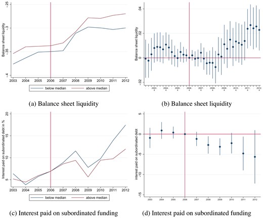
Bank level: Balance sheet liquidity and funding costs on subordinated debt. In this figure, we show mean dependent variables of raw data over time in the left column. In the right column, we show coefficient plots with confidence intervals at 90% from estimating equation (3) with annual data. Table 11 reports regression statistics for Figure 11b and Online Appendix Table B.6 reports the regression output for Figure 11d.
While balance sheet liquidity improves, we also document that covered bond issuance increases credit risk. It is therefore not clear how overall bank risk evolves. The risk premia asked by unsecured creditors provides us with an indication of the market’s perception of overall bank risk. In Figure 11c, we plot the average interest rate paid by banks for subordinated debt.23 After the introduction of covered bonds in 2007, we see a wedge building up between the two groups, with high-exposure banks showing on average lower funding costs on subordinated debt. In Figure 11d, we show results from estimating equation (3) with interest paid on subordinated debt as dependent variable. High-exposure banks pay lower funding costs on subordinated debt compared with other banks and the difference is statistically significantly different from zero at the 5% level in 2008 and 2009.24 We conclude that covered bond issuance reduces bank risk, suggesting that any positive effects from increased balance sheet liquidity offset any potential increase in credit risk due to more firm lending.
4.2.2. Bank Profitability
Finally, covered bonds have sizable effects on bank profitability. In Figure 12a, we show the evolution of average total funding costs over time and in Figure 12b, the coefficient plot from estimating equation (3) with interest paid on total funding as dependent variable. Covered bonds lower funding costs on secured debt, and as we have shown in the previous paragraph also on subordinated debt. This is reflected in the evolution of total funding costs: High-exposure banks pay lower total funding costs compared with other banks. The negative differential effect is statistically significantly different up to the 1% level in 2011.25
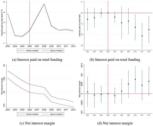
Bank level: Total funding costs and profitability. In this figure we show mean dependent variables of raw data over time in the left column. In the right column we show coefficient plots with confidence intervals at 90% from estimating equation (3) with annual data. Online Appendix Table B.6 reports the regression output for Figure 12b and d.
In Figure 12c, we assess net interest margins defined as net interest income over total assets as a measure of banks’ profitability. Net interest margins decrease for both groups,26 but less so for high-exposure banks. In fact, there is a mild positive differential effect as we show in Figure 12d.27
We conclude that issuing covered bonds not only reduces overall bank risk, but also reduces total funding costs by reducing interest paid by banks and therefore increases banks’ profitability.
4.3. Inspecting the Mechanism
In this section, we outline a simple model to theoretically analyze the mechanisms through which covered bond issuance can induce a reallocation of credit away from mortgages to corporate loans such as the one documented above. We then show support for some of the testable predictions of the model.
4.3.1. Summary of a Stylized Model of Bank Lending and Covered Bonds
In Online Appendix A, we present a stylized model to clarify how a risk-neutral bank adjusts its portfolio and risk-taking in response to an asset encumbrance technology such as covered bonds. The asset encumbrance technology improves the liquidity of the assets that are subject to potential encumbrance. The bank provides two products that meet creditors’ different risk appetites: a safe demand deposit contract with non-state contingent return backed by encumbered safe assets (call it mortgage lending) and a risky financial security with state-contingent return backed by a risky project (call it firm lending). Ideally, the bank prefers to invest more funds in risky firm lending since it has a higher expected return, but this increases volatility in asset return, making it more uncertain whether the bank is able to meet depositors’ demand for liquidity. As a response, depositors charge a higher risk premium when banks invest more in firm loans. In equilibrium, the optimal credit allocation of the bank equates the marginal gain from firm lending by the marginal increase in the risk premium.
Asset encumbrance technology, such as covered bonds, is modeled as an increase in cash generated from mortgages. This generates two diverting effects on the optimal credit allocation: on the one hand, there is an income effect that encourages the bank to invest more in safer mortgages as the return from mortgage lending increases. However, there is also a substitution effect that encourages the bank to engage more in riskier firm lending due to the enhanced funding liquidity. This liquidity effect occurs because more liquid assets reduces the risk premium that depositors charge banks when engaging in firm lending. If the risk aversion of depositors is very high and/or firm risk is high, the bank would choose to invest more in mortgage lending to reduce asset return volatility and the risk premium, i.e. the return effect dominates. If the risk aversion of depositors is very low and/or firm risk is sufficiently low, the bank would invest more in risky firm lending for higher profit. Since firm risk is something we can approximate using firm-level ratings, we test whether the shift to firm lending is higher for firms with lower firm risk as captured by their credit rating and refer to this testable hypothesis as H1.
Banks Facing Lower Firm Risk Shift More to Firm Lending.
Such effect is particularly strong for banks with a high cost of creating liquidity. In the lens of our model, we would therefore expect to see a larger shift from mortgages to firm loans following the introduction of covered bonds for banks with a high cost of creating liquidity. We test this hypothesis by investigating whether the shift to firm-lending is stronger for banks with lower holdings of net liquid assets, where the latter is a proxy for cost of creating liquidity. We refer to this testable hypothesis as H2.
Banks with Low Net Liquid Asset Holdings Shift More to Firm Lending.
We now turn to test these predictions.
4.3.2. Heterogeneous Effects of the Introduction of Covered Bonds
H1: Credit risk. The first testable prediction of our model is that banks are more likely to switch to firm lending when the returns from doing so are high. In our model, the bank is risk-neutral, so a higher marginal return on firm credit would incentivize banks to engage more in firm lending. In fact, for most banks and in most time periods, firm lending is more profitable than mortgage lending. In 92% of bank-year observations, the approximated interest rate on firm lending is higher than on other lending.28 Further, according to SSB (Statistics Norway) the average interest rate margin on loans to non-financial corporations between 2014q1 and 2021q1 was 2.22% and while it was 1.60% on mortgages, which also reflects higher yields on firm lending on average. However, according to our model, banks have to balance higher yields from firm lending with higher funding costs due to higher risk premia. We examine prediction H1 from our model that banks rather turn to firm lending if credit risk is relatively low. We observe data on firm rating for the universe of firms in our firm loan level data, and measure credit risk according to the mean rating of banks’ corporate borrowers in the pre period.
We show in blue in Figure 13a that banks whose borrowers carried lower risk in the pre period (red, high firm rating), decrease the share of mortgages over total lending more than banks exposed to higher firm risk. In Figure 13b, we show that the increase in firm lending following the introduction of covered bonds is driven by banks with initially lower risk in firm lending. On average, these banks increase the share of firm lending by 3.9 percentage points as reported in Table 12, whereas banks with high-yield firm loans do not increase firm lending. We conclude that banks with lower initial credit risk have more credit risk capacity and hence increase firm lending to more risky borrowers as a response to the introduction of covered bonds.
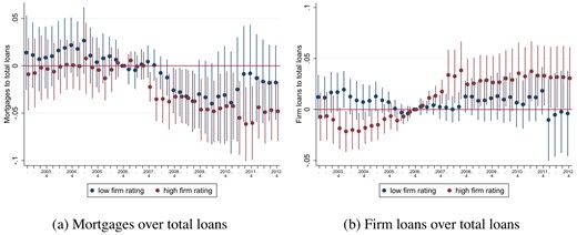
Bank portfolio re-balancing according to credit risk of firm lending. In these graphs, we show coefficient plots from re-estimating equation (3) for the sample of banks with high and low ratings with confidence intervals at 90%.
Regression information corresponding to Figure 10.
| Dependent variable | Figure | N | No. of banks | R2 | Mean of dep. var. | Sd of dep. var. |
|---|---|---|---|---|---|---|
| Securities over total assets | 10b | 5,150 | 133 | 0.378 | 0.089 | 0.045 |
| Dependent variable | Figure | N | No. of banks | R2 | Mean of dep. var. | Sd of dep. var. |
|---|---|---|---|---|---|---|
| Securities over total assets | 10b | 5,150 | 133 | 0.378 | 0.089 | 0.045 |
Notes: This table reports statistics from estimating equation (3). The second column (“Figure”) refers to the corresponding coefficient plot.
Regression information corresponding to Figure 11b.
| Dependent variable | Figure | Observations | N cluster | R2 | Mean dependent | SD dependent |
|---|---|---|---|---|---|---|
| Balance sheet liquidity | 11b | 5,150 | 133 | 0.447 | −0.324 | 0.074 |
| Dependent variable | Figure | Observations | N cluster | R2 | Mean dependent | SD dependent |
|---|---|---|---|---|---|---|
| Balance sheet liquidity | 11b | 5,150 | 133 | 0.447 | −0.324 | 0.074 |
Notes: This table reports statistics from estimating equation (3) with balance sheet liquidity as dependent variable. The second column (“Figure”) refers to the corresponding coefficient plot.
Summarizing portfolio rebalancing across banks.
| Change in portfolio share in pp of... | Low firm risk (high rating) | High firm risk (low rating) |
|---|---|---|
| Mortgages (relative to total loans) | −3.9** (1.6) | −3.1* (1.8) |
| Firm loans (relative to total loans) | 3.9** (1.8) | −0.1 (1.4) |
| Change in portfolio share in pp of... | Low firm risk (high rating) | High firm risk (low rating) |
|---|---|---|
| Mortgages (relative to total loans) | −3.9** (1.6) | −3.1* (1.8) |
| Firm loans (relative to total loans) | 3.9** (1.8) | −0.1 (1.4) |
Notes: This table summarizes the estimated treatment effect from estimating equation (3) splitting the sample according to firm loan risk measured according to firm rating in 2006. Robust standard errors are clustered at the bank level and are depicted in parentheses. *, **, *** indicate significant coefficients at the 10%, 5%, and 1% level, respectively.
H2: Net liquid asset holdings. We divide banks into two groups based on their 2006q4 ratio of net liquid assets to total assets as defined in Section 3.1 to test whether banks with low liquidity increase firm lending more than other banks. We then re-estimate equation (3) for the sample of low- and high-liquidity banks, respectively, using different bank level portfolio shares as dependent variables.
In Figure 14, we show the result from this exercise, using the share of mortgages (left panel) and firm loans (right panel). Starting with the left panel, the fraction of mortgages declines for high-exposure banks irrespective of whether we consider the low- or high-liquidity sample. In terms of magnitudes, however, the drop is roughly three times the size for banks in the low-liquidity sample. In Table 13, we summarize the average treatment effect over the post-2007q6 period within the low- and high-liquidity samples, respectively. In the sample of high-liquidity banks, the mortgage share decreases by approximately −2.0 percentage points on average. In the low-liquidity sample, however, the drop in the mortgage share is approximately −6.5 percentage points on average.
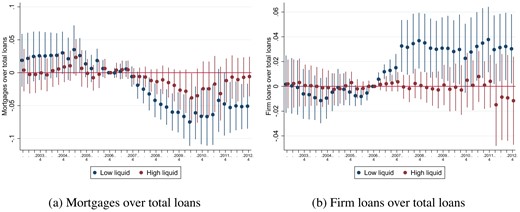
Bank portfolio re-balancing according to liquidity. In these graphs, we show coefficient plots from re-estimating equation (3) for the sample of low- and high-liquidity banks, respectively, with confidence intervals at 90%.
Summarizing portfolio rebalancing across banks.
| Change in portfolio share in pp of... | Low liquid banks | High liquid banks |
|---|---|---|
| Mortgages (relative to total loans) | −6.5*** (1.7) | −2.0 (1.3) |
| Firm loans (relative to total loans) | 3.3** (1.6) | −0.1 (1.1) |
| Change in portfolio share in pp of... | Low liquid banks | High liquid banks |
|---|---|---|
| Mortgages (relative to total loans) | −6.5*** (1.7) | −2.0 (1.3) |
| Firm loans (relative to total loans) | 3.3** (1.6) | −0.1 (1.1) |
Notes: This table summarizes the estimated treatment effect from estimating equation (3) splitting the sample according to liquidity in the pre-reform period. Robust standard errors are clustered at the bank level and are depicted in parentheses. *, **, *** indicate significant coefficients at the 10%, 5%, and 1% level, respectively.
In the right panel, we show the results focusing on firm lending. In this case, the results are starker—while there is no treatment effect in the high-liquidity sample, high-exposure banks in the low-liquidity sample increase the firm lending share by approximately 3.3 percentage points on average. Generally speaking, the larger treatment effects on firm lending are consistent with the model outlined above. Our results are in line with previous findings that liquidity is a constraint on firm lending (Webb 2000). Once liquidity improves, it is optimal for banks to provide more firm credit. The strong results suggest that covered bonds break up previous explicit or implicit liquidity constraints and enable sharp increases in firm lending.
4.4. Robustness
We address the concern of confounding demand shocks in our baseline approach at the loan level in Section 4.1.3 by including an extensive sets of FEs in our regression estimations to control for firm loan demand. Also, we control for systemic differences between banks with bank FEs in estimations at the bank level. Further, we observe whether differences between high-exposure and other banks change in the pre period, and can confirm that for most of our specifications the empirical evidence is consistent with parallel trends in the pre period. However, the analysis above cannot exclude the possibility that there are potentially other confounding supply-side (e.g. bank) shocks that affect our results. In Section 3.3, we discussed three potential concerns: exposure to the ongoing financial crisis, changes in relative risk aversion due to the financial crisis, and exposure to the capital requirement reduction due to the transition to Basel II. Below, we show the robustness of our results to these potentially confounding factors. Finally, we also present results with a continuous treatment measure in line with Callaway, Goodman-Bacon, and Sant’Anna (2024).
4.4.1. Exposure to the Financial Crisis
To investigate the correlation between our treatment measure and the exposure to the financial crisis, we compute a bank’s ratio of MM financial instruments to total assets and the ratio of interbank borrowing to total assets in 2006q4. These measures are aimed at capturing the two main channels of exposure to the financial crisis, as discussed in Section 3.3. In panels (a) and (b) in Figure C.4 in Online Appendix C, we plot these variables against our treatment measure, the share of eligible mortgages over total mortgages in 2006q4. For interpretation, we also include the regression coefficient from a univariate cross-sectional regression of the different variables on our treatment measure. In both cases, there is a weak and positive relationship between the exposure variable and our treatment measure. In both cases, we fail to reject the null hypothesis of no significant relationship.
4.4.2. Differences in Changes in Risk-Taking Behavior
Further, we want to rule out that our results are driven by differences in risk-taking behavior, which might change with the onset of the financial crisis as in Guiso, Sapienza, and Zingales (2018). In Figure C.5 in Online Appendix C, we show the correlation of our treatment measure and risk indicators in 2006q4. In particular, in Online Appendix Figure C.5a, we show the correlation of our treatment measure with total funding costs, in Online Appendix Figure C.5b with the changes in funding costs from 2006 to 2008 and in Online Appendix Figure C.5c with funding costs on unsecured debt. Less risk-averse banks should have higher funding costs and hence if high-exposure banks were more risk averse ex ante there should be a negative correlation with funding costs and our treatment measure. However, we find a very mild positive correlation with total funding costs. Moreover, there is no correlation with the change of funding costs at the onset of the financial crisis and with funding costs on subordinate debt.
As further indicators of risk-taking behavior, we show the correlation of our treatment measure with the standard deviation of return on assets over four quarters and over eight quarters in Online Appendix Figure C.5d and C.5e, respectively. If high-exposure banks were more prudent, we would expect them to have a lower standard deviation of return on assets. The correlations are close to zero. Further we show correlations with the share of liquid assets and the share of net liquid assets in Online Appendix Figure C.5f and C.5g, respectively. If high-exposure banks were more prudent before, we would expect to see a positive correlation with the share of liquid assets. There is only a mild negative correlation with net liquid assets.
Finally, we present three further measures to gauge the correlation between our treatment measure and bank risk. Banks with a larger share of eligible mortgage loans show lower equity ratios in 2006q4 in Online Appendix Figure C.5h. This in fact goes hand-in-hand with the definition of our treatment measure: banks that hold more high-quality loans do not need to hold more equity. Meanwhile these banks also have lower non-performing loan (NPL) ratios in Online Appendix Figure C.5i, which also reflects the fact that they have more high-quality mortgage loans on their balance sheets. According to these two indicators, banks seem on the one hand less risk-averse due to lower equity ratios, but on the other hand more risk-averse due to lower NPL ratios. There is only one indicator that might indicate higher risk aversion for high-exposure banks: banks with a higher share of eligible assets supply on average higher-rated firms, as can be seen in Online Appendix Figure C.5j.
4.4.3. Differences in Changes In Portfolio Diversification
A further concern could be that our high-exposure banks were less diversified before the onset of the financial crisis, and hence diversified their portfolio as a response to the financial crisis by increasing firm lending. We investigate the share of firm and mortgage lending over total assets and total lending, respectively, in Online Appendix Table B.1. There is no difference across the two groups in terms of specialization in one asset class. In Online Appendix Figure C.6, we also present the correlation of our continuous treatment measure with the share of mortgage lending over total assets in Online Appendix Figure C.6a, mortgage lending over total loans in Online Appendix Figure C.6b, as well as the share of firm lending over total assets in Online Appendix Figure C.6c and firm lending over total loans in Online Appendix Figure C.6d. Again, we do not observe differences across low- and high-exposure banks. We conclude that it is unlikely that high-exposure banks were less diversified in terms of firm versus mortgage lending before the financial crisis and reacted by increasing their firm lending.
4.4.4. Transition to Basel II
As discussed in Section 3.3, a further potential confounding factor could be the transition to Basel II. In panel (c) in Figure C.4 in Online Appendix C, we investigate the correlation with the capital requirement change due to the Basel II transition and our treatment measure. Specifically, the Basel II transition reduced capital requirements due to a reduction in average risk weights. The reduction in average risk weights was a function of banks’ initial portfolios. We therefore follow Juelsrud and Arbatli-Saxegaard (2020) and compute the reduction in average risk weights due to the Basel II transition for each bank, and multiply that with the headline capital requirement of 8% to get a measure of the actual capital requirement reduction for each bank. We then plot this measure against our treatment variable. There is a very weak and statistically insignificant relationship between the capital requirement reduction due to Basel II and the fraction of low LTV mortgages, supporting our identifying assumptions.
4.4.5. Including Controls
In addition to static evidence presented in scatter plots, we allow for dynamic impact on outcome variables of the exposure measures to the financial crisis, the transition to Basel II and indicators of risk-taking. In particular, we re-estimate equation (3) and include control variables (|$X_b$|) as their q42006 value and interact with indicators for every quarter-year.29
|$X_b$| include the share of MM assets over total assets, the fraction of interbank funding, capital requirement reduction due to Basel II, interest paid on total funding, standard deviation of return on assets over past four quarters, share of liquid assets ((MM assets + central bank reserves)/total assets), share of net liquid assets (((MM assets + central bank reserves) − interbank borrowings − certificates)/total assets), equity ratio, ratio of NPLs and log of total assets. We present coefficient plots in Online Appendix Figure B.3 and corresponding statistics in Table B.7 in Online Appendix B. Our results remain robust, and we conclude that the findings of our paper are not driven by differences in exposure to the financial crisis, to the transition to Basel II or due to differences in ex-ante risk-taking behavior.
4.4.6. Excluding Largest Banks
High exposure banks are on average larger than low exposure banks. To exclude that our results are merely driven by large, high exposure banks, we exclude the ten largest banks from the sample according to total assets in q42006 in estimations on the bank level. In this way, we can also rule out that the effect that we observe is driven by large banks who might be differently affected by the financial crisis compared to small banks. We show the results in Online Appendix Figure B.4 and corresponding statistics in Table B.8 in Online Appendix B. Our results do not change.
Also, we exclude largest banks in estimations on the loan level. We show the results in Online Appendix Figure B.5 and corresponding statistics in Table B.9 in Online Appendix B for excluding the three, five, and ten largest banks, respectively. As large banks have larger market shares, the number of observations reduces greatly. Still, we find that the growth of loans is larger from high exposure banks compared to low exposure banks after the covered bond market has opened up. We conclude that our findings are not driven by large banks only, or by the fact that large banks might have reacted differently to the financial crisis.
4.4.7. Continuous Treatment Measure
Throughout our analyses, we use a binary indicator to measure banks’ exposure to the introduction of covered bonds. For robustness, we use our actual continuous treatment measure, the share of eligible mortgages 2006q4, and re-estimate equation (3) in line with Callaway, Goodman-Bacon, and Sant’Anna (2024). We show the results in Figure B.2 and in Table B.5 in Online Appendix B. The results are consistent with the results in the preceding paragraphs.
5. Conclusion
How do banks rebalance their portfolios in response to the possibility of issuing covered bonds? Evidence on that question is rare so far. We aimed to fill this gap by analyzing the consequences of the introduction of covered bond issuance in Norway in June 2007. While some initial concerns were that covered bonds would lead to an expansion of mortgage credit, our main result shows that the opposite took place: banks reallocated funds from mortgages and to firm loans. However not all corporations benefit from the increases in loan supply. In particular, banks tailor new loan supply to ex ante younger and low-rated firms, thereby increasing credit risk. We further find that banks increase holdings of liquid assets and increase total balance sheet liquidity. We assess risk premia asked by unsecured creditors and find that total bank risk decreases: lower liquidity risky outweighs higher credit risk.
We can reconcile previous contradictory findings in the literature on whether covered bonds increase or decrease banks’ risk taking by carving out conditions under which banks shift to more firm lending. We sketch out a model that predicts that banks with low initial liquidity would use the possibility of covered bonds to raise liquidity to extend more risky lending such as firm lending. Further, in the model credit risk needs to be sufficiently low. We find empirical evidence consistent with the predictions of the model.
Our paper raises related issues for future research. One is whether the impact of covered bond issuance on bank lending differs under different institutional and market setups. As our theoretical model predicts, our finding that banks rebalance portfolios from mortgages to firm loans is context-specific and depends on several deep parameters, such as default risk in the firm sector. Our paper thus encourages cross-country studies for a better understanding of how covered bonds influence market outcomes.
Acknowledgments
We thank Jonas Hjort (Editor), three anonymous referees, Santiago Barraza, Michael Cook, Reint Gropp, Joar Johnsen, Michael Koetter, Felix Noth, Daniel Streitz, Olav Syrstad, seminar participants at Sveriges Riksbanken, TU Dresden, Lund University, University of Essex, Bank of Lithuania, Bank of Slovakia, Norges Bank, Stockholm Business School, ZEW Mannheim, NBRE Spring Institute, Otto-von-Guercke University of Magdeburg, IWH Halle, and conference participants at ASSA 2022 Annual Meeting, the meeting of the German Finance association (DGF), the Econometric Society European winter meeting, the FMA European Conference, as well as an anonymous referee for the Norges Bank Working Paper series for their valuable comments and suggestions. This paper should not be reported as representing the views of Norges Bank. The views expressed are those of the authors and do not necessarily reflect those of Norges Bank. Cao is affiliated at CESifo. Juelsrud is affiliated at CEPR.
Notes
The editor in charge of this paper was Jonas Hjort.
Footnotes
This “originate and distribute” aspect of ABS might potentially affect banks incentive to monitor borrowers and assess credit risk in a very different way compared to a case where the assets are retained on bank balance sheets, as in the case of asset encumbrance. See Jiménez et al. (2020), Chakraborty, Goldstein, and MacKinlay (2018), Mian and Sufi (2009), Purnanandam (2011), and Carbó-Valverde, Rosen, and Rodríguez-Fernández (2017).
Data extracted from European Covered Bond Council (2020) and European Central Bank Statistical Data Warehouse.
The harmonization of covered bond markets across Europe was one of the main goals of the European capital markets union. Since July 2022, all new issuances are affected by the new Covered Bond Directive (CBD). Meanwhile, covered bond issuance in 2022 exceeded all previous years (S&P 2023). Covered bonds are therefore also expected to play an increasingly important role in the banking system going forward.
We also discuss and address other potential confounding factors in Section 3.3.
As of the end of 2018, 97% of covered bonds outstanding in Norway are backed by residential mortgages (Finance Norway 2018). The other 3% are backed by commercial mortgages and public sector loans. Therefore, in this paper, we focus on mortgage loans as the collateral of covered bonds.
Importantly, any assets transferred to a mortgage company remain on-balance sheet for the bank on a consolidated basis, in contrast to for instance ABS before the financial crisis.
Banks in countries such as Denmark, Germany, or Spain have long histories of covered bond issuance, whereas there was a wave of covered bond market introductions starting in the 2000s in Finland (2000), Ireland (2001), Sweden (2004), Portugal (2006), Italy and Greece (2007), and in the UK and the Netherlands (2008) (European Central Bank 2008).
Nine banks enter the market during our sample period.
Among the shared mortgage companies, Eika Boligkreditt AS has the most owners and is shared by 81 banks. SpareBank1 Boligkreditt AS follows with 20 owning banks. The remaining shared mortgage companies are co-owned by few banks.
According to household-level information, around 3% of loans in 2008 had an LTV between 75% and 80%, see Aastveit, Juelsrud, and Wold (2022). As such, the measurement error associated with observing loans below 80% and not 75% is likely to be limited.
We consolidate balance sheet positions from banks with their mortgage companies on the basis of the share of mortgage transfers to the mortgage company. As this is only an approximation of the exact positions, it might be that the sum of average ratios exceeds 1. In two instances, total loans over total assets exceeded 1. We set these two observations to missing. Note further that one bank has incomplete reports on firm loans during the pre period, hence we have twelve observations less.
Limited liability firms represent the vast majority of the Norwegian private sector. In most of the years in our sample, these firms employ roughly 90% of the private sector labor force.
Approximately USD 324,000. 1 USD = 8.58 NOK on 5 March, 2021.
AAA (coded as 1) is the top rating a firm can achieve, while C (coded as 5) is the worst rating.
Note that we slightly overestimate the share of eligible mortgages for all banks in our sample and hence might introduce a slight measurement error in |$T_b$|. As noted in Section 3.1, on average all banks have 3% of mortgages between LTV 75% and 80%, which can inform about the potential maximum measurement error.
A primary reason why banks did not transfer all eligible mortgages, were to ensure that the credit quality of the remaining portfolio did not deteriorate too much.
The risk weight on loans in the retail portfolio was lowered from 100% to 75%. The risk weight on mortgages with an LTV below 80% was reduced from 50% to 35%.
See results in Section 4.4.
Evidence so far demonstrates an increase in credit supply on the intensive margin. We also test for differences at the extensive margin and present results on the number of firms or loans, as well as changes thereof, at the bank level in Table B.3 in Online Appendix B. We do not find differences across high and low exposure banks on these dimensions. We conclude that it is the intensive margin of loan supply that is affected by the introduction of covered bonds.
High-exposure banks increase balance sheet liquidity compared with low-exposure banks by up to 0.03 percentage points. Given that mean balance sheet liquidity for high exposed banks in the pre period is −0.34, the relative increase corresponds to 8.8% of the latter.
Note that yearly data such as the banks’ income statements that we use to construct the funding cost measures are reported in annual frequency and that not all banks use subordinated debt in every period, hence the number of observations is reduced.
High-exposure banks reduce funding costs on subordinated debt compared with other banks by up to 4.79 percentage points. Given that mean funding costs in the pre period for high-exposure banks is 5.70%, the relative decrease corresponds to 84% of the latter.
High-exposure banks reduce their total funding costs in the post period compared with other banks by up to 21 basis points. Given that average funding costs in the pre-period for high-exposure banks is 2.38%, the relative reduction corresponds to 8.8% of the latter.
The average decrease in net interest margin is likely tied to the decline in average interest rate which typically is associated with general compression of interest margins, see for instance Abadi, Brunnermeier, and Koby (2023).
High-exposure banks increase their net interest margin in the post period compared with low-exposure banks by up to 0.001. Given that mean interest margins in the pre-period for high-exposure banks is 0.022, the relative increase corresponds to 4.5% of the latter.
We approximate the average interest rate on firm lending per bank from our loan level data set as in equation (2) and average over all firm–bank observations per bank in 2006. We derive interest on all other lending by subtracting total interest paid by firms per bank from total interest income from loans in banks’ income statements and divide it by total lending minus total firm lending.
