


Abstract
In recent decades, there has been an increase in the share of males struggling in the labor market and education. We show in a set of large-scale experimental studies involving more than 35,000 Americans that people are more accepting of males falling behind than they are of females falling behind, and less in agreement with government policies supporting males falling behind. We provide evidence of the underlying mechanism being statistical fairness discrimination: People consider males falling behind to be less deserving of support than females falling behind because they are more likely to believe that males fall behind due to lack of effort. These findings are important for understanding how society perceives and responds to the growing number of disadvantaged males.
Teaching Slides
A set of Teaching Slides to accompany this article is available online as Supplementary Data.
1. Introduction
Men continue to dominate top-level positions across the world, and a significant gender wage gap remains in all societies. In the United States (US), women working full-time earned, on average, 83% of what men did on an annual basis in 2021 (US Bureau of Labor Statistics 2022). Consequently, there is an urgent need for political action to achieve gender equality for women.
The present paper is motivated by a different gender gap that has emerged in the labor market and education in recent decades (Autor and Wasserman 2013). In high-income countries, there is growing concern about the prospects for low-skilled males: “The decline in economic opportunities for low-skilled men and the possible negative effects of this trend on their well-being is a matter of increasingly urgent concern for policy makers and the general public” (Coile and Duggan 2019, p. 2). Males with less than a 4-year college education have experienced a significant reduction in real income over the last decade in the US (Autor and Wasserman 2013; Binder and Bound 2019), and the percentage of young and prime-age males outside the labor force in the US has increased (Blau and Kahn 2013; Krueger 2017). The prospects for males outside the labor force are dim, particularly for those from low-income households and for males with minority backgrounds. The likelihood of living in poverty has increased and their expected future health and emotional well-being is poor (Autor and Wasserman 2013; Council of Economic Advisers 2016; Krueger 2017). In countries within the Organisation for Economic Co-operation and Development (OECD), males face heightened risks from self-destructive behaviors, evidenced by suicide, severe alcohol misuse, and drug overdose rates that are almost four times higher than those of females (OECD 2020). Males are also more susceptible to violent fatalities, with homicide rates markedly higher for males (4.4 per 100,000) than for females (0.9 per 100,000), compounded by greater exposure to harmful risk factors such as excessive tobacco and alcohol use (OECD 2023; OECD Better Life Index 2024).
There is also growing concern about boys falling behind in education. In most OECD countries, a larger share of boys than girls do not attain the baseline level of proficiency in any of the core subjects of mathematics, reading, and science (OECD 2015). In the US, for instance, the average percentage of students who do not attain the baseline proficiency level is 71% higher for boys than for girls. Boys are also dropping out of high school at higher rates than girls in most OECD countries. In higher education, females have surpassed males in graduation rates in nearly all OECD countries, on average by 12 percentage points (OECD 2022).
These striking developments make it important to study how people perceive and react to males falling behind, which is likely to shape policies targeting disadvantaged males in both the public and the private sector. In this paper, we report from a large-scale experimental study of how people’s fairness preferences and beliefs depend on the gender of the person falling behind. In particular, we are interested in whether there is statistical fairness discrimination against males falling behind: Do people consider males falling behind to be less deserving of support than females falling behind because they are more likely to believe that males fall behind due to lack of effort than females? In the first part of the paper, we provide choice experimental evidence on whether people are more accepting of inequalities when males fall behind than when females fall behind in a controlled work environment, and whether people believe to a greater extent that males fall behind due to lack of effort compared with females in this environment. In the second part, we report from a corresponding survey experiment to study whether the findings in the choice experiment carry over to the policy domain. In total, more than 35,000 Americans participated in the different experiments in this study.
To gather choice experimental data from a representative sample of the general population in the US, we leverage the infrastructure of a leading international data-collection agency along with an online labor market (Almås, Cappelen, and Tungodden 2020). In the online labor market, we recruit workers and create inequalities by paying two workers differently for the same assignment. In our main treatments, the inequality is generated by paying the more productive worker more than the less productive worker. We then ask a general population sample of Americans to act as third-party spectators and make consequential decisions about whether to redistribute earnings between the two workers. Spectators are randomly assigned to a treatment where the low-productive worker is a male or to a treatment where the low-productive worker is a female. Our main interest is in studying whether the redistribution decisions of the spectators depend on the gender of the low-productive worker. We run a set of additional treatments to shed light on the underlying mechanisms of the spectators’ choices, where we vary the source of the inequality (merit or luck) and the gender composition of the two workers (mixed gender or single gender). In an independent general population sample of Americans, we elicit beliefs about the effort exerted by the males and females who fall behind in the choice experiment. Finally, we conduct a follow-up study where participants make both a spectator choice and state beliefs about effort, and also provide the main reason for their redistribution decision in an open-text response.
To study statistical fairness discrimination in the policy domain, we implement a large-scale survey experiment that investigates whether support for government policies targeting people falling behind depends on the gender of those falling behind, and whether beliefs about effort are different for males and females falling behind in the labor market and education.
Our findings provide compelling evidence of males falling behind being treated differently than females falling behind, both in the choice experiment and in the survey experiment, and of the underlying mechanism being statistical fairness discrimination. The main findings are illustrated in Figure 1. In a controlled work environment, a significantly higher share of people choose not to transfer anything to a male falling behind due to low productivity than to a female falling behind, 38.4% versus 31.1% (Panel a), and a significantly higher share of people believe that males fall behind in the choice experiment due to lack of effort than females, 53.0% versus 44.3% (Panel b). These findings are similarly reflected in the survey experiment: Fewer people express support for government assistance to males falling behind than to females falling behind in the labor market and education, 54.2% versus 42.2% (Panel c), and more people believe that males fall behind in the labor market and education due to lack of effort than females, 46.7% versus 32.5% (Panel d). The treatment effect of manipulating the gender in the choice experiment is comparable with the treatment effect of manipulating the gender in the survey experiment. The magnitude of the gender treatment effect is in most cases comparable with the difference between Republicans and non-Republicans.
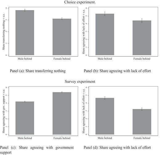
Main findings. Panel (a) shows the share of participants transferring nothing to the male falling behind and the female falling behind in the mixed-gender merit treatments. Panel (b) shows the share of participants who strongly or somewhat agree with the statement “I expect that the less productive man (woman) exerted less effort on the assignment than the more productive woman (man).” Panel (c) shows the share of participants who strongly or somewhat agree with the statement “It is very important that the government provides support to males (females) who fall behind in education and in the labor market.” Panel (d) shows the share of participants who strongly or somewhat agree with the statement “When males (females) fall behind in education and in the labor market, it largely reflects their lack of effort” or the statement “Males (Females) falling behind in education and in the labor market have exerted low effort.” The panels are based on independent samples. The standard errors are indicated by the bars.
The findings are robust across subgroups in society, to different experimental manipulations and empirical specifications, and to multiple hypothesis testing. In the follow-up experiment, we also provide additional evidence of effort beliefs shaping the gender bias. The gender bias in the share transferring nothing to the low-productive worker nearly halves when we control for effort beliefs, and there is a significant larger share of people stating that the person falling behind is less deserving when the male is falling behind than when the female is falling behind. Taken together, the evidence strongly suggests that statistical fairness discrimination is an important mechanism for understanding how Americans relate to males falling behind.
Our paper contributes to several important literatures. The findings augment the growing literature on the negative developments of males in the labor market and education. The existing literature has documented how the low performance of males reflects structural changes and socioeconomic developments (Rosin 2012; Autor and Wasserman 2013; Bertrand and Pan 2013; Almås et al. 2016; Krueger 2017; Autor et al. 2019; Binder and Bound 2019), and the present paper complements these findings by providing novel evidence on how society perceives males who fall behind. We show that people believe that it is more likely that males falling behind have exerted low effort than females falling behind, which may result in males falling behind being treated differently in school, in the workplace, and in the family.
We further contribute to the literature on gender discrimination (Bertrand and Duflo 2017), by showing how males who fall behind may face statistical fairness discrimination. Although important papers document discrimination against females in different domains, such as in hiring decisions (Bohren et al. 2025; Goldin and Rouse 2000; Coffman, Exley, and Niederle 2021), task allocation (Babcock et al. 2017), bargaining (Castillo et al. 2013; Exley, Niederle, and Vesterlund 2020), teaching evaluations (Mengel, Sauermann, and Zölitz 2019), and career development (Reuben, Sapienza, and Zingales 2014), recent studies highlight discrimination against males in certain settings (Williams and Ceci 2015; Bohren, Imas, and Rosenberg 2019; Mengel, Sauermann, and Zölitz 2019; Reynolds et al. 2020; Feess, Feld, and Noy 2021). Notably, Bohren, Imas, and Rosenberg (2019) find in a field experiment on an online mathematics forum for students and researchers in STEM fields (Science, Technology, Engineering, and Mathematics) that females initially encounter significant discrimination but gradually become favored over men. Our paper focuses specifically on males who fall behind in a distributive context. In a large-scale study of the general population in the US, we demonstrate that people are less willing to support males falling behind than females falling behind. Furthermore, we contribute to the discrimination literature by presenting evidence of the underlying mechanism being statistical fairness discrimination, with people in their fairness considerations making inferences about whether a worker is deserving of support based on their background characteristics.1 Statistical fairness discrimination is likely to extend beyond the distributive setting explored in our study, and may be relevant for understanding discriminatory behavior in any context where a principal would like to reward effort.
Finally, our results contribute to the literature in behavioral economics, specifically to understand the role of gender considerations in people’s social preferences (Eckel and Grossman 2008; Croson and Gneezy 2009). Prior studies have investigated the effect of varying the salience of the recipient’s gender in dictator games and ultimatum games. A meta-study on dictator game experiments finds that females receive higher allocations compared with males in dictator games when the gender of the recipient is made salient (Engel 2011). In ultimatum games that manipulate the gender of the recipient, individuals tend to make higher offers to males compared with females (Eckel and Grossman 2001; Solnick 2001). In contrast to these earlier studies, we examine gender discrimination in third-party spectator choices, which provides a direct expression of participants’ moral preferences (Cappelen et al. 2013). In this setting, we demonstrate significant statistical fairness discrimination against males. We also provide new evidence on how fairness preferences shape distributive behavior (Fehr and Schmidt 1999; Bolton and Ockenfels 2000; Konow 2000; Bortolotti et al. 2025; Cappelen et al. 2007; Cappelen, Falch, and Tungodden 2020; Dong, Huang, and Lien 2022; Falch 2022; Hvidberg, Kreiner, and Stantcheva 2023; Andre 2025), by showing how people’s fairness considerations differ across contexts and the characteristics of the workers. Finally, the study contributes to the behavioral literature by providing unique large-scale evidence on how gender influences inequality acceptance in a general population sample.
The remainder of the paper is organized as follows: Section 2 presents the experimental designs, Section 3 outlines the empirical strategy. The main results from the choice experiment are reported in Section 4, and the findings from the survey experiment are presented in Section 5. Section 6 concludes. Additional analysis and the complete instructions for the experiments are provided in the online appendices.
2. Research Design and Participants
We report from two large-scale experimental studies examining people’s acceptance of males falling behind. The first study is a choice experiment, where third-party spectators decide whether to redistribute earnings from a more productive worker with high earnings to a less-productive worker with no earnings. The second study is a survey experiment where participants state their level of agreement with the government providing support to people falling behind in the labor market and education. Both studies employ a between-subject design where we manipulate the gender of those falling behind, which allows us to causally identify whether people are less concerned about males falling behind compared with females falling behind. To study whether statistical fairness discrimination can explain the observed patterns, we elicit beliefs about the effort exerted by those who fall behind, both in a sample where the participants have not made a spectator choice and, in a follow-up study, in a sample where the participants have made a spectator choice. The full study was implemented through a series of data collections in collaboration with high-quality international survey providers2; see Online Appendix B.1 for further details. We implemented three rounds of the main choice experiment, with a pre-analysis plan specified for each round (registered at the AEA RCT Registry: AEARCTR-0000853, AEARCTR-0001027, and AEARCTR-0005610). The main analysis is in line with the pre-registered empirical strategy and hypotheses. In Online Appendix A.4, we provide a discussion of how and when we deviate from the pre-analysis plans. We did not specify separate pre-analysis plans for the other parts of the study, because they mirror the spectator design in the choice experiment. The instructions for the different parts of the study can be found in Online Appendix B.
2.1. Choice Experiment
We provide here the structure of the choice experiment, which builds on Almås, Cappelen, and Tungodden (2020). First, workers were recruited to complete an assignment.3 Second, the workers were matched in pairs and assigned different earnings. Third, the spectators were randomly matched to a pair of workers and decided whether to redistribute earnings between the two workers. Finally, the workers were paid according to the spectators’ decisions. Online Appendix Table A.1 summarizes the main stages of the spectator design.
In all treatments, the spectators were presented with a situation where one worker had earnings of 6 USD and the other had earnings of 0 USD. They were informed that both workers were from the US and were of the same age. The spectators were not informed about the nature of the tasks assigned to the workers. It was emphasized to the spectators that, unlike traditional survey questions, their choice was consequential. To minimize the role of worker expectations, the spectators were told that the workers would not at any point be informed about their initial earnings.
In the two main treatments, referred to as the mixed-gender merit treatments, the spectators consider a distributive situation involving a female worker and a male worker. The initial inequality in earnings in the merit treatments is determined by the productivity of the workers: The spectators were informed that the more productive worker earns 6 USD and the less productive worker earns 0 USD. The only difference between the two merit treatments is whether the low-productive worker is a male or a female. This experimental design allows us to causally identify whether spectators are more inequality accepting when a male is falling behind compared with when a female is falling behind. To provide further evidence on how the source of inequality affects the spectators’ concern for the worker falling behind, we also implemented two mixed-gender luck treatments that mirrored the two main treatments but where the inequality in earnings was determined by luck. Finally, to investigate the effect of the gender composition of the worker pair on the spectators’ behavior, we implemented four single-gender treatments that mirrored the four mixed-gender treatments. We employed a between-subject design, where spectators were randomly assigned to treatments; see Table 1 for an overview.4
Choice experiment: Treatments.
| Spectator choice | |||||
|---|---|---|---|---|---|
| Mixed-gender | Single-gender | ||||
| Female behind | Male behind | Female behind | Male behind | ||
| Source of | Merit | T1 | T2 | T5 | T6 |
| inequality | Luck | T3 | T4 | T7 | T8 |
| Spectator choice | |||||
|---|---|---|---|---|---|
| Mixed-gender | Single-gender | ||||
| Female behind | Male behind | Female behind | Male behind | ||
| Source of | Merit | T1 | T2 | T5 | T6 |
| inequality | Luck | T3 | T4 | T7 | T8 |
Notes: The table provides an overview of the eight treatments in the choice experiment. We collected the data in three main rounds. First, we recruited 2,052 participants, who were randomly allocated to one of eight treatments. Second, we recruited 1,050 participants, who were randomly allocated to one of the two mixed-gender merit treatments. Third, we recruited 11,419 participants, who were randomly allocated to one of the four mixed-gender treatments. In the first and second round, spectators were matched uniquely with a pair of workers who would be paid in accordance with their decision; in the third round, one out of ten spectator decisions were randomly selected and implemented for a pair of workers. In independent samples with 3,000 participants, we additionally elicited effort beliefs for the choice experiment, where the participants were randomly allocated to one of six treatments (T1–T6). In the follow-up study, we recruited 5,000 participants, who were randomly allocated to one of the four mixed-gender merit treatments (one out of ten spectator decisions were randomly selected and implemented for a pair of workers).
To examine beliefs about the effort exerted by the worker falling behind, we conducted an independent survey involving a distinct sample of participants who were randomly assigned to one of the treatments in the choice experiment. We implemented this survey on a different sample than the choice experiment to avoid any confounds between the spectators’ choices and elicited beliefs.5 The participants were asked to state the extent to which they agreed with the following statement: “I expect that the less productive man (woman) exerted less effort than the more productive woman (man),” on a scale from 1 (strongly disagree) to 5 (strongly agree). References to productivity were only part of the statement for participants assigned to one of the merit treatments. The luck treatments, on the other hand, mirrored the absence of such signals for the spectators and provided no information about productivity.6 This part of the design allows us to causally identify, within the controlled work environment of the choice experiment, whether people believe that males are more likely than females to fall behind due to lack of effort.
To further study the robustness of our findings and explore underlying mechanisms, we conducted a follow-up study where the participants were randomly assigned to make a distributive decision in one of the mixed-gender merit treatments (with a male or a female as the low-productive worker). Different from the main study, the spectators were then asked to state the main reason for their choice, and the extent to which they agreed that the low-productive worker had exerted low effort. This approach enables us to study whether and how effort beliefs predict spectator choices, the potential mediating effect of these beliefs, and the participants’ stated justification for their decisions.
2.2. Survey Experiment
In the survey experiment, participants were asked whether they agreed with the government providing support to people falling behind in the labor market and education. In a between-subject design, we randomly manipulated the gender of those who fall behind. Specifically, the participants were presented with the following statement: “It is very important that the government provides support to males (females) who fall behind in the labor market and education,” and then responded on a scale from 1 (strongly disagree) to 5 (strongly agree).
To elicit beliefs about the role of effort of people falling behind in the labor market and education, we employed two different approaches. In one study, we asked participants about the role of effort in explaining why some fall behind: “We observe some males (females) falling behind in education and in the labor market. To what extent do you agree with the statement: When males (females) fall behind in education and in the labor market, it largely reflects their lack of effort.” In a second study, we asked directly about their beliefs about the level of effort of people falling behind: “We observe some males (females) falling behind in education and in the labor market. To what extent do you agree with the statement: Males (Females) falling behind in education and in the labor market have exerted low effort.” For both questions, the participants responded on a scale from 1 (strongly disagree) to 5 (strongly agree). The two questions allow us to identify whether people are more likely to believe that males fall behind due to lack of effort in the labor market and education, and whether these beliefs are sensitive to the exact formulation of the question. Online Appendix Table A.2 provides an overview of the treatment design in the survey experiment.
2.3. Participants
We collected background characteristics from all participants in terms of gender, age, income, and political orientation. Table 2 presents an overview of the background characteristics of the participants by experiment and a comparison with US census data. We observe that there are only small differences in the background characteristics of the participants in the choice experiment and in the survey experiment. The samples are fairly balanced in terms of gender, with about 47% males. The median age of the participants is 46 years and the median yearly household income before taxes is around 50,000 USD. About one-third of the participants state that they would vote Republican. Overall, the samples are largely representative of the US population (+18 years old) on these dimensions, even though we note that income is more compressed in the samples than in the population at large (which may partly reflect that self-reported income was restricted at the extremes). We use population weights to account for various demographic factors in our main analysis, using population statistics and estimates from the US Census Bureau to determine the weighting targets. In Online Appendix Tables A.3–A.6, we show that the samples are balanced across treatments.
Descriptive statistics.
| Choice | Survey | US | |
|---|---|---|---|
| experiment | experiment | ||
| Male (share) | 0.472 | 0.463 | 0.487 |
| Age (year) | |||
| Median | 46 | 46 | 47 |
| p10 | 24 | 23 | 23 |
| p90 | 70 | 69 | 73 |
| Income (USD) | |||
| Median | 55,700 | 48,000 | 63,600 |
| p10 | 12,500 | 17,500 | 12,800 |
| p90 | 137,500 | 117,900 | 179,600 |
| Republican (share) | 0.354 | 0.313 | 0.280 |
| N | 22,521 | 13,264 |
Notes: The table reports the descriptive statistics for the participants in the choice experiment, including the follow-up experiment, and in the survey experiment, and for the US population. Samples (self-reported): The income variable is yearly household income in USD before taxes (inflation adjusted to 2020), given in standard categories where we impute the midpoint in each group to calculate the average. For the highest and lowest income groups, we impute 1.5 times the lower boundary and 0.5 times the higher boundary, respectively (see Online Appendix Section B.7 for a list of income categories). The participants who did not know or did not want to state their income are not included in the descriptives on income (261/17,521 and 371/13,264 observations, respectively). A participant is classified as Republican if he or she would have voted for the Republican party if there was an election tomorrow. US population: The share of males and the median age (+18) in the US are estimates from the US Census Bureau, American Community Survey (2018 and 2019) (https://www.census.gov/ and https://www.census.gov/data/). The income data are based on 2018 estimates from the US Census Bureau, American Community Survey (inflation adjusted to 2020). Political affiliation is from Gallup (http://news.gallup.com/poll/).
3. Empirical Strategy
In the main analysis of the choice experiment, we focus on the following empirical specification:
where |$u_i$| is an indicator for whether spectator i has transferred nothing to the worker with no earnings or the standardized amount transferred, |$\it {Male\, behind}_i$| is an indicator variable for the spectator being in a treatment where a male has fallen behind, |$Luck_i$| is an indicator for the spectator being in a treatment where the inequality in earnings is determined by luck, |$\it {Male\, behind} \times \it {Luck}_i$| is an interaction variable between the two treatment indicators, |${\bf X}_i$| is a vector of control variables, and |${\epsilon }_i$| is an error term. We report equation (1) with and without the set of control variables (gender, political affiliation, income, and age), and separately for the mixed-gender treatments and the single-gender treatments. Correspondingly, when analyzing elicited beliefs about the effort exerted by the two workers, we estimate (1) with the dependent variable being an indicator for whether the spectator agrees (somewhat or strongly) that the worker with no earnings has exerted less effort than the worker with earnings, or the standardized level of agreement (strongly disagree (1) − strongly agree (5)).
We study heterogeneous effects in the spectators’ decisions and elicited beliefs for the gender, political orientation, income, and age of the participants. To illustrate, we use the following specification when studying gender differences in the mixed-gender merit treatments:
where |$u_i$| is the relevant dependent variable (spectator’s decision or elicited beliefs), |$M_{i}$| is an indicator variable for participant i being male, and |$M_{i} \times \it {Male\, behind}_{i}$| is an interaction variable for the participant being male and in a treatment where a male worker has no earnings. In this analysis, we only report results for the standardized dependent variable, but the findings are robust to using the corresponding indicator variable.
The analysis of the survey experiment follows the same structure as for the choice experiment, but the main regression equation is simplified because we do not manipulate why people fall behind in the survey experiment. Hence, we estimate the following regression:
where |$u_i$| is the relevant dependent variable (policy support or elicited beliefs) and |$\it {Male\, behind}_i$| is an indicator variable for participant i being in a treatment where the question is about males falling behind in the labor market and education. We report equation (3) with and without the same set of control variables as in the analysis of the choice experiment. We consider two dependent variables when studying policy support: an indicator variable for whether the participant agrees (somewhat or strongly) that the government should provide support to people falling behind in the labor market and education or the standardized level of agreement (strongly disagree (1) – strongly agree (5)). Correspondingly, we consider both an indicator variable and the standardized level of agreement when studying beliefs about effort. The two versions of the belief question give very similar results (see Online Appendix Figure A.4), and thus we pool them in the main analysis. In the heterogeneity analysis of the survey experiment, we estimate a version of equation (2) with the relevant dependent variables for policy support and elicited beliefs.
In the analysis of both the choice experiment and the survey experiment, we compute p-values adjusted for multiple hypothesis testing as a robustness check of the main results. We calculate unadjusted p-values as bootstrap p-values following Davison and Hinkley (1997), and compute p-values adjusted for step-down multiple testing following the algorithm proposed by Romano and Wolf (2016). Bootstrapping is implemented with 10,000 replications. All the main findings are robust to multiple hypothesis testing, as shown in Online Appendix A.2.
4. Choice Experiment: Results
We first provide an overview of the spectators’ decisions and beliefs about effort in the choice experiment, before we turn to the regression analysis of the main treatments and the heterogeneity analysis.
4.1. Descriptive Statistics
Figure 2 gives an overview of the distributions of the spectators’ transfers (upper panel) and beliefs about effort (lower panel) pooled for all treatments; see Online Appendix Figures A.1–A.2 for the corresponding distributions by treatment.
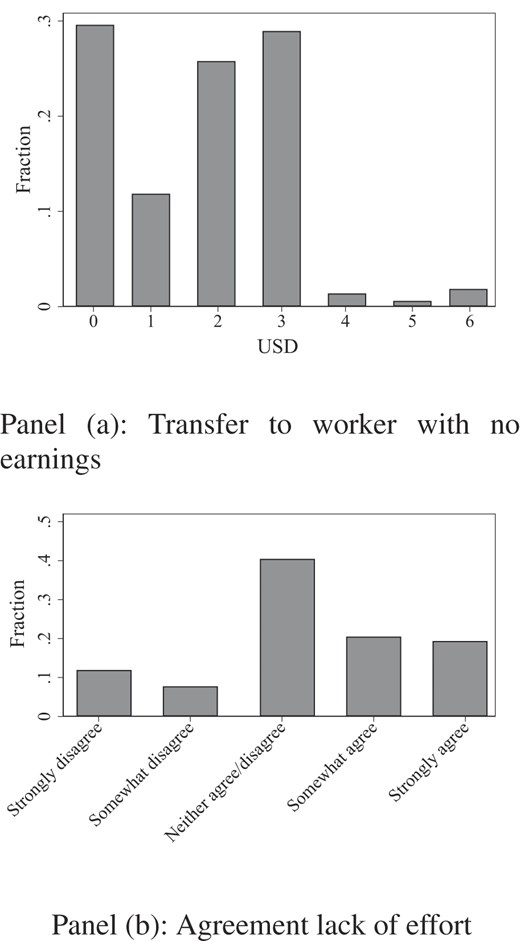
Choice experiment. Panel (a) shows the distribution of transfers (in USD) to the worker falling behind, pooled for all treatments. Panel (b) shows the extent of agreement with the worker falling behind having exerted less effort than the worker ahead, pooled for all treatments. The two panel are based on independent samples.
From the upper panel, we observe that the most common spectator allocations are to give nothing to the worker with no earnings (30%) and to equalize the earnings (29%). The large majority of spectators (67.2%) give more to the worker with earnings than to the worker with no earnings, whereas very few spectators (4%) give more to the worker with no earnings. The lower panel shows that about 40% of the participants strongly or somewhat agree that the worker with no earnings has exerted less effort than the worker who is ahead. The mode is neither to agree nor to disagree, while about 20% somewhat or strongly disagree.
4.2. Main Findings
We start by discussing the regression analysis of the mixed-gender treatments (merit and luck), where the initial inequality in earnings between a male worker and a female worker is determined by the productivity of the workers or by luck. Table 3 reports the estimates of equation (1), where columns (1)–(4) report the regression analysis for the spectators’ redistributive decisions and columns (5)–(8) report the regression analysis for the elicited beliefs about effort.
Choice experiment.
| Spectator choice | Effort beliefs | |||||||
|---|---|---|---|---|---|---|---|---|
| Nothing to | Amount to | Agree | Level of | |||||
| worker behind | worker behind (std) | low effort | agreement (std) | |||||
| Male behind | 0.073|$^{***}$| | 0.074|$^{***}$| | −0.129|$^{***}$| | −0.130|$^{***}$| | 0.087|$^{***}$| | 0.089|$^{***}$| | 0.216|$^{***}$| | 0.217|$^{***}$| |
| (0.012) | (0.012) | (0.024) | (0.024) | (0.033) | (0.033) | (0.057) | (0.057) | |
| Luck | −0.079|$^{***}$| | −0.077|$^{***}$| | 0.480|$^{***}$| | 0.476|$^{***}$| | −0.271|$^{***}$| | −0.261|$^{***}$| | −0.816|$^{***}$| | −0.796|$^{***}$| |
| (0.012) | (0.012) | (0.026) | (0.026) | (0.029) | (0.029) | (0.064) | (0.062) | |
| Luck |$\times$| Male behind | −0.040|$^{**}$| | −0.042|$^{**}$| | 0.061|$^{*}$| | 0.067|$^{*}$| | 0.011 | 0.003 | 0.328|$^{***}$| | 0.314|$^{***}$| |
| (0.017) | (0.017) | (0.037) | (0.036) | (0.043) | (0.042) | (0.086) | (0.084) | |
| Male participant | 0.039|$^{***}$| | −0.057|$^{***}$| | 0.034 | 0.094|$^{**}$| | ||||
| (0.009) | (0.018) | (0.022) | (0.044) | |||||
| Republican | 0.087|$^{***}$| | −0.189|$^{***}$| | 0.015 | 0.036 | ||||
| (0.009) | (0.019) | (0.022) | (0.044) | |||||
| Low income | −0.005 | 0.054|$^{***}$| | −0.040|$^{*}$| | −0.050 | ||||
| (0.009) | (0.018) | (0.022) | (0.043) | |||||
| Low age | −0.029|$^{***}$| | 0.038|$^{**}$| | 0.178|$^{***}$| | 0.365|$^{***}$| | ||||
| (0.009) | (0.018) | (0.022) | (0.043) | |||||
| Constant | 0.310|$^{***}$| | 0.276|$^{***}$| | −0.168|$^{***}$| | −0.118|$^{***}$| | 0.443|$^{***}$| | 0.356|$^{***}$| | 0.215|$^{***}$| | 0.009 |
| (0.009) | (0.012) | (0.018) | (0.024) | (0.023) | (0.030) | (0.042) | (0.056) | |
| Male behind (luck) | 0.033|$^{***}$| | 0.031|$^{***}$| | −0.067|$^{**}$| | −0.063|$^{**}$| | 0.098|$^{***}$| | 0.092|$^{***}$| | 0.544|$^{***}$| | 0.531|$^{***}$| |
| (0.012) | (0.012) | (0.028) | (0.028) | (0.027) | (0.026) | (0.064) | (0.062) | |
| Observations | 13,495 | 13,495 | 13,495 | 13,495 | 1,998 | 1,998 | 1,998 | 1,998 |
| |$R^{2}$| | 0.016 | 0.028 | 0.069 | 0.081 | 0.087 | 0.123 | 0.150 | 0.185 |
Notes: The table reports population-weighted linear regressions where the dependent variable is an indicator variable for the spectator transferring nothing to the worker who is falling behind (columns (1)–(2)), the standardized amount transferred to the worker who is falling behind (columns (3)–(4)), an indicator variable for the participant strongly or somewhat agreeing with the worker falling behind having exerted less effort than the worker ahead (columns (5)–(6)), and the standardized level of agreement with the worker falling behind having exerted less effort than the worker ahead (columns (7)–(8)). The standardized variables are established on the basis of the responses by the participants in the respective mixed-gender treatments (T1–T4). Spectator choices and effort beliefs are elicited in independent samples. “Male behind” is an indicator variable for the participant being in the treatment where the male is falling behind. “Male participant” is an indicator variable for being male. “Republican” is an indicator variable for voting Republican. “Low income” is an indicator variable for having an income below the median income per year in the respective sample. “Low age” is an indicator variable for being below 46 years old (which is the median age in the pooled sample). “Luck” is an indicator variable for the participant being in a treatment where luck is the source of inequality. “Luck |$\times$| Male behind” is an interaction between “Luck” and “Male behind”. The regressions in columns (1)–(4) include indicator variables for the round of the study in which the spectator took part (not reported). Robust standard errors in parentheses: *p |$<$| 0.10, **p |$<$| 0.05, ***p |$<$| 0.01.
In column (1), we observe a significant effect of manipulating the gender of the worker with no earnings on the spectators’ choices in the merit treatments: The share of spectators transferring nothing to the low-productive worker with no earnings increases by 7.3 percentage points when this worker is a male rather than a female. In column (2), we show that the estimated treatment effect is robust to including background variables for the gender of the spectator, political orientation, income, and age, and, in columns (3)–(4), that it is robust to using the standardized amount transferred as the dependent variable. The standardized amount transferred to the worker with no earnings is reduced by about 0.13 standard deviations when the low-productive worker is a male rather than a female. We note that the estimated treatment effect of manipulating the gender of the worker with no earnings is as large as the gap between Republicans and non-Republicans when considering the share of spectators transferring nothing to the worker with no earnings, and two-thirds of the gap between Republicans and non-Republicans when considering the amount transferred.
In columns (5)–(8), we find a corresponding pattern for elicited beliefs in the merit treatments. In column (5), we observe that the share of participants agreeing that the worker with no earnings has exerted less effort than the worker with earnings increases with 8.7 percentage points when the low-productive worker is a male rather than a female, which is close to the estimated treatment effect on the share of participants giving nothing to the worker with no earnings (column (1)). Hence, the evidence suggests that more participants transfer nothing to low-productive males with no earnings than to low-productive females with no earnings in the merit treatments because they are more likely to believe that low productive males have exerted low effort than low-productive females. The estimated treatment effect of manipulating the gender of the low-productive worker on beliefs about effort is robust to including background characteristics (column (6)), and to using the standardized level of agreement as the dependent variable (columns (7)–(8)). We find that the level of agreement increases by about 0.22 standard deviations when the worker with no earning is a male rather than a female.
We summarize these findings as our first main result.
People redistribute less to a low productive male with no earnings than to a low productive female with no earnings, and people agree more that a low productive male has exerted low effort than a low productive female.
In Figure 3, we report the estimated treatment effects on the spectators’ choices and elicited beliefs by subgroup for the mixed-gender merit treatments; see Online Appendix Tables A.8–A.9 for the complete set of regression estimates. In Panel (a), we observe that the estimated treatment effect on the amount transferred to the low-productive worker with no earnings is negative and significant in all subgroups. Hence, across subgroups, we find that people transfer less to a low-productive male with no earnings than to a low-productive female with no earnings. We do not find significant differences in the spectators’ choices across subgroups. In Panel (b), we report the corresponding heterogeneity analysis for beliefs about effort. We observe that the estimated treatment effect on the level of agreement is positive for all subgroups, which means that, across subgroups, we find that participants agree more that the low-productive worker has exerted low effort when the low-productive worker is a male rather than a female. The estimated treatment effect is significant for all subgroups, except for males and young participants. We summarize these findings as our second main result:
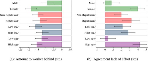
Choice experiment, heterogeneity, mixed-gender merit. Panel (a) reports, by subgroup, the estimated treatment effect for the standardized amount transferred to the low-productive worker with no earnings in the mixed-gender merit treatments (T1 and T2). Panel (b) reports, by subgroup, the estimated treatment effect for the standardized level of agreement with the low-productive worker having exerted low effort in the mixed-gender merit treatments (T1 and T2). The estimates are from population-weighted linear regressions as specified in equation (2), where we run separate regressions for the background variables “Male participant,” “Republican,” “Low income,” and “Low age,” as defined in Table 3. In all regressions, we include the relevant background variable and its interaction with “Male behind.” The regressions underlying Panel (a) also include indicators for the round of the study in which the spectator took part. Spectator choices and effort beliefs are elicited in independent samples. Robust standard errors are indicated by bars.
In all subgroups in the population, we find less willingness to redistribute and more agreement with the low productive worker with no earnings having exerted low effort when the low productive worker is a male rather than a female.
Table 3 further studies how the spectators’ choices and elicited beliefs are affected by manipulating the source of inequality. We observe that when the initial earnings are determined by luck rather than merit, the share of spectators transferring nothing decreases significantly (columns (1)–(2)), and that the transferred amount increases significantly (columns (3)–(4)), in line with the existing evidence in the literature (Almås, Cappelen, and Tungodden 2020). We observe that there is a significant interaction effect between the source of the inequality and the gender of the worker with no earnings. The gender effect on the share transferring nothing and on the transferred amount is larger in the mixed-gender merit treatments than in the mixed-gender luck treatments. However, even in the mixed-gender luck treatments, we find that more people transfer nothing and that the transferred amount is smaller when a male has no earnings than when a female has no earnings.
In columns (5)–(8) in Table 3, we report the elicited beliefs for the mixed-gender luck treatments. We observe that, as expected, the share of participants agreeing that the worker with no earnings has exerted less effort than the worker with earnings decreases significantly when the earnings have been allocated randomly. However, also in the mixed-gender luck treatments, participants believe that it is more likely that a male with no earnings has exerted low effort than a female with no earnings, which implies that participants believe that it is more likely that the average male worker has exerted less effort than the average female worker (given that earnings is an uninformative signal about productivity in the luck treatments). The fact that the participants transfer less to a male with no earnings than to a female with no earnings also in the luck treatments is thus consistent with statistical fairness discrimination: the participants believe even in the luck treatment that it is more likely that a male has exerted low effort than a female. The gender effect on the share agreeing that the worker with no earnings has exerted low effort is in fact equally large in the mixed-gender luck treatments as in the mixed-gender merit treatments.7 Hence, the fact that the gender effect on the transfer to the worker with no earnings is lower in the luck treatments than in the merit treatments, despite beliefs about the gender difference in effort being the same, suggests that people consider it more justifiable to accept an inequality based on effort considerations in the merit treatments than in the luck treatments.
We also implemented a set of single-gender treatments (merit and luck) in the first round of data collection, to study the effect of the gender composition of the pair of workers on the spectators’ choices, see Online Appendix Table A.10 for details. We do not find any evidence of the gender of the two workers having a significant effect on the share transferring nothing or on the amount transferred to the worker with no earnings in either the single-gender merit treatments or the single-gender luck treatments. Hence, it is not the case that people generally treat males and females differently, this pattern only emerges when they consider a distributive situation involving both a male worker and a female worker. Further, consistent with statistical fairness discrimination, we also show in Online Appendix Table A.10 that people’s beliefs about the effort of the low-productive worker in the single-gender merit treatments do not depend on whether they consider two male workers or two female workers. Finally, in Online Appendix Table A.11, we show that male workers with no earnings receive less and are more likely to receive nothing in the mixed-gender merit treatments than in the single-gender merit treatments, whereas female workers with no earnings are treated in the same way in the mixed-gender merit treatments and the single-gender merit treatments. Taken together, the evidence suggests that people consider males who are less productive than females to be particularly undeserving of support because they consider it a strong signal of a male having exerted low effort if a male is less productive than a female.
4.3. Follow-up Experiment
In this section, we report from a follow-up study that examines the robustness of the identified gender bias in the mixed-gender treatments; whether effort beliefs mediate the gender bias; and how spectators justify their redistribution choices in open-text responses.
In columns (1)–(8) in Table 4, we show that the follow-up study replicates the findings in the main study. First, the share of spectators transferring nothing to the low-productive worker increases by 5.0 percentage points when this worker is male rather than female (columns (1)–(2)), and the standardized amount transferred is reduced by 0.062 standard deviations (columns (3)–(4)). Second, the share agreeing that the low-productive worker has exerted low effort increases by 13.6 percentage points when the low-productive worker is a male rather than a female (columns (5)–(6)), and the standardized level of agreement increases by 0.324 standard deviations (columns (7)–(8)). The estimated effects are robust to including background characteristics.
Follow-up, choice experiment.
| Spectator choice | Effort beliefs | Both | ||||||||||
|---|---|---|---|---|---|---|---|---|---|---|---|---|
| Nothing to | Amount to | Agree | Level of | Nothing to | Amount to | |||||||
| worker behind | worker behind (std) | low effort | agreement (std) | worker behind | worker behind (std) | |||||||
| Male behind | 0.050|$^{***}$| | 0.051|$^{***}$| | −0.062|$^{**}$| | −0.063|$^{**}$| | 0.136|$^{***}$| | 0.135|$^{***}$| | 0.324|$^{***}$| | 0.324|$^{***}$| | 0.026|$^{*}$| | 0.026|$^{**}$| | −0.005 | −0.006 |
| (0.013) | (0.013) | (0.028) | (0.028) | (0.014) | (0.014) | (0.028) | (0.028) | (0.013) | (0.013) | (0.028) | (0.028) | |
| Male participant | 0.013 | −0.008 | 0.031|$^{**}$| | 0.069|$^{**}$| | 0.008 | 0.004 | ||||||
| (0.013) | (0.028) | (0.014) | (0.028) | (0.013) | (0.028) | |||||||
| Republican | 0.077|$^{***}$| | −0.182|$^{***}$| | 0.065|$^{***}$| | 0.105|$^{***}$| | 0.069|$^{***}$| | −0.164|$^{***}$| | ||||||
| (0.014) | (0.029) | (0.015) | (0.030) | (0.014) | (0.029) | |||||||
| Low income | −0.000 | 0.070|$^{**}$| | −0.012 | −0.000 | −0.000 | 0.070|$^{**}$| | ||||||
| (0.014) | (0.029) | (0.014) | (0.028) | (0.013) | (0.028) | |||||||
| Low age | −0.035|$^{***}$| | 0.094|$^{***}$| | 0.074|$^{***}$| | 0.102|$^{***}$| | −0.042|$^{***}$| | 0.112|$^{***}$| | ||||||
| (0.013) | (0.028) | (0.014) | (0.028) | (0.013) | (0.028) | |||||||
| Level of agreement (std) | 0.076|$^{***}$| | 0.075|$^{***}$| | −0.177|$^{***}$| | −0.176|$^{***}$| | ||||||||
| (0.007) | (0.007) | (0.015) | (0.015) | |||||||||
| Constant | 0.316|$^{***}$| | 0.301|$^{***}$| | 0.031 | 0.019 | 0.431|$^{***}$| | 0.362|$^{***}$| | −0.162|$^{***}$| | −0.282|$^{***}$| | 0.328|$^{***}$| | 0.322|$^{***}$| | 0.002 | −0.031 |
| (0.009) | (0.015) | (0.019) | (0.033) | (0.010) | (0.016) | (0.020) | (0.034) | (0.009) | (0.015) | (0.019) | (0.032) | |
| Observations | 5000 | 5000 | 5000 | 5000 | 5000 | 5000 | 5000 | 5000 | 5000 | 5000 | 5000 | 5000 |
| |$R^{2}$| | (0.003) | (0.011) | (0.001) | (0.013) | (0.018) | (0.028) | (0.026) | (0.032) | (0.028) | (0.035) | (0.031) | (0.043) |
Notes: The table reports linear regressions where the dependent variable is an indicator variable for the spectator transferring nothing to the worker who is falling behind (columns (1), (2), (9), and (10)), the standardized amount transferred to the worker who is falling behind (columns (3), (4), (11), and (12)), an indicator variable for the participant strongly or somewhat agreeing with the worker falling behind having exerted less effort than the worker ahead (columns (5) and (6)), and the standardized level of agreement with the worker falling behind having exerted less effort than the worker ahead (columns (7) and (8)). The latter is also used as a control variable in columns (9)–(12), “Level of agreement (std).” The standardized variables are established on the basis of the full follow-up sample (T1–T2). “Male behind” is an indicator variable for the participant being in the treatment where the male is falling behind. “Male participant” is an indicator variable for being male. “Republican” is an indicator variable for voting Republican. “Low income” is an indicator variable for having an income below the median income per year in the follow-up sample. “Low age” is an indicator variable for being below the median age in the follow-up sample. Robust standard errors in parentheses: *p |$<$| 0.10, **p |$<$| 0.05, ***p |$<$| 0.01.
In the follow-up study, we elicited beliefs from the spectators who made redistribution choices, which allows us to provide further evidence on the underlying mechanism of the gender bias in transfers. In columns (9)–(12), we observe that there is a strong positive correlation between effort beliefs and the amount transferred to the person falling behind. Further, we find that the estimated gender bias on the share transferring nothing to the worker falling behind is almost halved when including effort beliefs, and completely eliminated for the standardized amount transferred. Taken together, these patterns are consistent with meritocratic spectators transferring less to males falling behind because they believe that they have exerted less effort.
In the follow-up study, participants were also asked to describe the main reason for their redistribution choice. Following Bursztyn et al. (2023), we categorized the answers to the open-ended question using two methods: manual coding and large language models (GPT via OpenAI API). Based on this categorization, we identify the share of participants who refer to the least productive worker as relatively less deserving than the most productive worker when justifying their choice; see Online Appendix A.3 for further details. In Figure 4, we report the average share of participants who refer to the person falling behind as less deserving than the person ahead in each of the two mixed-gender merit treatments. We observe that the share of people justifying their redistribution choice with the less productive being less deserving is 19% higher (3.4 percentage points, |$p=0.003$|) if the person falling behind is a male rather than a female. The results are robust to including background variables, and to using API-coded data instead of hand-coded data. This mirrors the gender bias we find in redistribution behavior and stated effort beliefs, and is consistent with the underlying mechanism for the gender bias being statistical fairness discrimination.

Main reasons. Person behind relatively undeserving. Panel (a) shows the share of participants who find the person falling behind less deserving than the person ahead, by the gender of the person behind, using hand-coded data. Panel (b) shows the same using data coded by a large language model (GPT). The sample in both panels are the participants in the follow-up experiment. The standard errors are indicated by the bars.
5. Survey Experiment: Results
In this section, we study whether people are more accepting of males falling behind than females falling behind when considering support for governmental interventions, and whether they believe that males to a greater extent than females are falling behind in the labor market and education due to lack of effort. We first provide an overview of the policy attitudes and beliefs, before we turn to the regression analysis of the treatment effects and the heterogeneity analysis.
5.1. Descriptive Statistics
Figure 5 gives an overview of the distributions of the policy attitudes (upper panel) and beliefs about effort (lower panel) pooled for whether the question is about males or females falling behind; see Online Appendix Figure A.3 for the corresponding distributions by treatment.
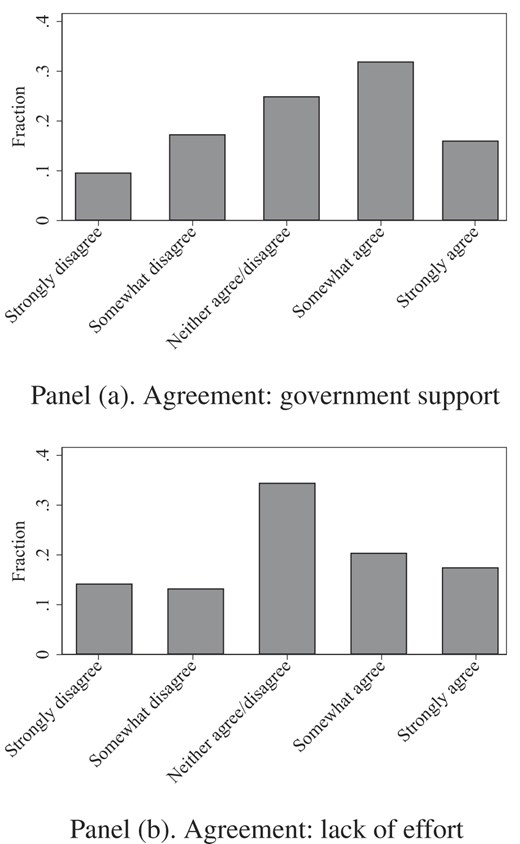
Survey experiment. Panel (a) shows the distribution of agreement with the statement “It is very important that the government provides support to males (females) who fall behind in education and in the labor market.” Panel (b) shows the distribution of agreement with the statement “When males (females) fall behind in education and in the labor market, it largely reflects their lack of effort” or the statement “Males (Females) falling behind in education and in the labor market have exerted low effort.” In both panels, the level of agreement is measured on a scale from strongly disagree (1) to strongly agree (5). The two panels are based on independent samples.
From the upper panel, we observe that there is disagreement about this type of government interventions: 27.0% of the participants strongly or somewhat disagree with these governmental policies, whereas 48.0% strongly or somewhat agree. In the lower panel, we observe that there is a corresponding disagreement in the beliefs about whether people are falling behind in the labor market and education largely due to their lack of effort: 27.5% strongly or somewhat disagree, whereas 38.0% strongly or somewhat agree.
5.2. Main Findings
We start by discussing the regression analysis of how the gender of the person falling behind affects policy attitudes and beliefs about effort. Table 5 reports the estimates of equation (3), where columns (1)–(4) report the regression analysis for the participants’ policy attitudes and columns (5)–(8) report the regression analysis for the elicited beliefs about effort.
Survey experiment.
| Government support | Effort beliefs | |||||||
|---|---|---|---|---|---|---|---|---|
| Agree important | Level of | Agree | Level of | |||||
| to support | agreement (std) | low effort | agreement (std) | |||||
| Male behind | −0.119|$^{***}$| | −0.117|$^{***}$| | −0.272|$^{***}$| | −0.266|$^{***}$| | 0.141|$^{***}$| | 0.141|$^{***}$| | 0.462|$^{***}$| | 0.463|$^{***}$| |
| (0.009) | (0.009) | (0.019) | (0.018) | (0.022) | (0.021) | (0.046) | (0.043) | |
| Male participant | 0.017|$^{*}$| | 0.013 | 0.118|$^{***}$| | 0.203|$^{***}$| | ||||
| (0.009) | (0.018) | (0.022) | (0.044) | |||||
| Republican | −0.199|$^{***}$| | −0.506|$^{***}$| | 0.130|$^{***}$| | 0.321|$^{***}$| | ||||
| (0.010) | (0.020) | (0.023) | (0.046) | |||||
| Low income | 0.031|$^{***}$| | 0.115|$^{***}$| | −0.112|$^{***}$| | −0.217|$^{***}$| | ||||
| (0.009) | (0.018) | (0.022) | (0.044) | |||||
| Low age | 0.124|$^{***}$| | 0.285|$^{***}$| | 0.191|$^{***}$| | 0.371|$^{***}$| | ||||
| (0.009) | (0.018) | (0.022) | (0.043) | |||||
| Constant | 0.542|$^{***}$| | 0.523|$^{***}$| | 0.136|$^{***}$| | 0.102|$^{***}$| | 0.270|$^{***}$| | 0.132|$^{***}$| | −0.230|$^{***}$| | −0.507|$^{***}$| |
| (0.007) | (0.010) | (0.013) | (0.020) | (0.019) | (0.027) | (0.042) | (0.060) | |
| Observations | 11,209 | 11,209 | 11,209 | 11,209 | 2,054 | 2,054 | 2,054 | 2,054 |
| |$R^{2}$| | 0.014 | 0.071 | 0.018 | 0.106 | 0.033 | 0.119 | 0.053 | 0.136 |
Notes: The table reports population-weighted linear regressions where the dependent variable is an indicator variable for the participant strongly or somewhat agreeing with “It is very important that the government provides support to females (males) who fall behind in education and in the labor market” (columns (1)–(2)), the standardized level of agreement with the same statement (columns (3)–(4)), an indicator variable for the participant strongly or somewhat agreeing with the statement “When females (males) fall behind in education and in the labor market, it largely reflects their lack of effort” or the statement “Females (Males) falling behind in education and in the labor market have exerted low effort” (columns (5)–(6)), and the standardized level of agreement with the same statements (columns (7)–(8)). The standardized variables are established on the basis of the responses by the participants in the respective treatments (P1 and P2). Policy preferences and effort beliefs are elicited in independent samples. “Male behind,” “Male participant”, “Republican”, “Low income,” and “Low age” are defined in Table 3. Robust standard errors in parentheses: *p |$<$| 0.10, **p |$<$| 0.05, ***p |$<$| 0.01.
In column (1), we observe a significant effect of manipulating the gender of people falling behind on support for government interventions: The share of participants agreeing with government interventions is reduced by 11.9 percentage points when those falling behind are males rather than females. In column (2), we show that the estimated treatment effect is robust to including background variables for the gender of the participant, political orientation, income, and age, and in columns (3)–(4) that it is robust to using the standardized level of agreement as the dependent variable. The standardized level of agreement is reduced by about 0.27 standard deviations when the question is about the government providing support to males falling behind rather than to females falling behind, which is an even larger gender effect than we observe in the redistributive decisions in the choice experiment (see Table 3). We note that the estimated treatment effect of manipulating the gender of those falling behind on the support for government interventions is about half of the gap between Republicans and non-Republicans, both in terms of the share agreeing with government interventions and the standardized level of agreement.
In columns (5)–(8), we find a corresponding pattern for elicited beliefs about effort. In column (5), we observe that the share of participants agreeing that those falling behind have exerted low effort increases by 14.1 percentage points when those falling behind are males rather than females, which is close to the estimated reduction in the share of participants agreeing with government interventions when those falling behind are males rather than females (column (1)). Hence, as in the choice experiment, we observe that the estimated effect on beliefs about effort is comparable with the estimated effect on the acceptability of the inequality. Thus, the evidence suggests that fewer participants support government interventions when males fall behind than when females fall behind because they are more likely to believe that males falling behind have exerted low effort than have females falling behind. The estimated treatment effect of manipulating the gender of those falling behind on beliefs about effort is robust to including background characteristics (column (6)), and to using the standardized level of agreement as the dependent variable (columns (7)–(8)). We find that the standardized level of agreement increases by about 0.46 standard deviations when those falling behind are males rather than females, which is even greater than the effect on beliefs about effort when manipulating the gender in the choice experiment. The estimated treatment effect of manipulating the gender of those falling behind on beliefs about effort is comparable with the estimated gap between Republicans and non-Republicans, both in terms of the share agreeing to those falling behind having exerted low effort and the standardized level of agreement. Taken together, we state the following result:
People agree less with the government providing support to males falling behind in the labor market and education than to females falling behind, and people agree more that males falling behind have exerted low effort than females falling behind.
In Figure 6, we report the estimated treatment effects on policy attitudes and beliefs about effort by subgroup, see Online Appendix Tables A.12–A.13 for the complete set of regression estimates. In Panel (a), we observe that the estimated treatment effect on the agreement with government interventions supporting those who fall behind is negative and significant in all subgroups. Hence, across subgroups, we find that people agree less with government interventions when a male rather than a female is falling behind. We find that the gender effect is smaller for males compared with females, Republicans compared with non-Republicans, and younger participants compared with older participants. In Panel (b), we report the corresponding heterogeneity analysis for beliefs about effort. We observe that the estimated treatment effect on the level of agreement is positive for all subgroups, which means that, across subgroups, we find that participants agree more that males falling behind have exerted low effort than females falling behind. We find the largest difference in the estimated treatment effect on beliefs about effort between young and older participants, with the older participants differentiating their beliefs about the effort significantly more based on the gender of those falling behind. This may reflect that older generations have been shaped by potentially stronger gender stereotypes in society. We summarize the heterogeneity analysis in the following result:
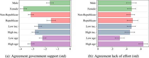
Survey experiment, heterogeneity. Panel (a) reports, by subgroup, the estimated treatment effect for the standardized level of agreement with the government providing support for people falling behind in education and in the labor market (P1 and P2). Panel (b) reports, by subgroup, the estimated treatment effect for the standardized level of agreement with people falling behind in the labor market and education having exerted low effort (P1 and P2). Policy preferences and effort beliefs are elicited in independent samples. The estimates are from population-weighted linear regressions as specified in equation (2), where we run separate regressions for the background variables “Male participant,” “Republican,” “Low income,” and “Low age,” as defined in Table 3. All regressions include the relevant background variable and its interaction with “Male behind”. The regressions underlying Panel (b) also include indicators for the round of the study in which the spectator took part. Robust standard errors are indicated by bars.
In all subgroups in the population, we find less agreement with the government providing support and more agreement with those falling behind in the labor market and education having exerted low effort when considering males falling behind compared with females falling behind.
6. Concluding Remarks
In recent decades, disadvantaged males have experienced a downward trajectory in the labor market and education in many countries, which partly reflects structural changes and socioeconomic developments (Autor and Wasserman 2013). How society responds to this development may depend critically on how we perceive males who fall behind. We have shown in a set of large-scale experimental studies conducted with general population samples from the US that people are more accepting of males falling behind than females falling behind, and we provide evidence suggesting that this greater acceptance reflects that people consider males falling behind to be less deserving of support than females falling behind. We find these patterns in both a large-scale choice experiment studying redistribution in a controlled work environment and a large-scale survey experiment studying people’s agreement with policy interventions supporting those who fall behind in the labor market and education. In a follow-up experiment, we find that the identified gender bias in transfers is significantly reduced and even disappears when controlling for beliefs about effort, and that spectators are more likely to express that the person falling behind is less deserving when it is a male rather than a female. Taken together, the observed pattern may be seen as reflecting statistical fairness discrimination based on a meritocratic fairness view: People are more accepting of males falling behind than females falling behind because they are more likely to believe that males fall behind due to low effort than females.
Statistical fairness discrimination may shed light on a wide range of discriminatory behavior. To illustrate, consider the accumulated non-experimental evidence suggesting, albeit with some exceptions, that teachers’ grade setting is biased against males in a range of subjects in kindergarten, primary school, high school, and higher education (Lavy 2008; Cornwell, Mustard, and Van Parys 2013; Falch and Naper 2013; Breda and Ly 2015; Lindahl 2016; Lavy and Sand 2018; Terrier 2020). Such behavior may reflect statistical fairness discrimination, where teachers may be more likely to interpret poor performance of male students to reflect lack of effort than poor performance of female students. It would be of great interest in future research to explore statistical fairness discrimination in field studies in education and in the workplace, and establish more evidence on its relevance for explaining gender discriminatory behavior. It is also important to further our understanding of why people view lack of effort to be a more likely explanation for why males fall behind than for why females fall behind, and to understand how this difference in perception relates to stereotypes that people have about males and females (Alan, Ertac, and Mumcu 2018; Bordalo et al. 2019).
We have focused on how statistical fairness discrimination may disadvantage males falling behind, but, in different contexts, this mechanism may disadvantage females. For example, affirmative action for females may make people less supportive of females falling behind if affirmative action policies make people believe that females who fall behind have exerted low effort. It may also contribute to explain the recent global evidence suggesting relatively low support in gender equal societies for affirmative action to promote women in leadership positions (Bursztyn et al. 2024). More broadly, statistical fairness discrimination may contribute to explaining other types of discrimination, including discrimination against ethnic minorities and immigrants (Cettolin and Suetens 2019), where people may hold stereotypes about the effort exerted by these groups.
We have suggested an experimental paradigm for studying statistical fairness discrimination that is applicable to a wide range of different domains (see also Haeckl, Möller, and Zednik (2023)). An interesting avenue for future research would be to study how the gender bias depends on the nature of the task and the particular context, and the extent to which it reflects misperceived beliefs about effort and ability. We hope that future research also will use this experimental approach to deepen our understanding of how statistical fairness discrimination shapes behavior and policies. In an era where politics has become “a personal responsibility crusade” (Hacker 2006), we need to carefully examine how we relate to people who are struggling in society (Moffitt 2015; Bursztyn et al. 2024; Schildberg-Hörisch et al. 2023).
Acknowledgments
The study was organized by the Centre for Experimental Research on Fairness, Inequality, and Rationality (FAIR) at the Department of Economics, NHH Norwegian School of Economics. We thank Editor Chris Roth and three anonymous referees for valuable comments and suggestions. We are grateful to Daniel Benjamin, Pedro Rey Biel, Caroline Bonn, Gary Charness, Stefano DellaVigna, Catherine Eckel, Christine L. Exley, Uri Gneezy, Ingar Haaland, Alex Imas, Siri Isaksson, Elisabeth Ivarsflaten, Nanjundi Karthick Krishnan, James Konow, Erin Krupka, Erzo F.P. Luttmer, Axel Ockenfels, Anders Poulsen, Odile Poulsen, Lise Rakner, Imran Rasul, Charlotte Ringdal, Kjell Salvanes, Marta Serra-Garcia, Ingrid Hoem Sjursen, Charles Sprenger, Eirik Strømland, Matthias Sutter, Jonas Tungodden, Lise Vesterlund, and numerous seminar participants for valuable comments and suggestions and to Morgane Bakehe, Sigurd Dyrstad, Sebastian Fest, and Eivind Bang Støeng for valuable research assistance. We are also thankful for the financial support from the New Opportunities for Research Funding Agency Cooperation in Europe Network (NORFACE), The Centre for Ethics and Economics at the Norwegian School of Economics, the Research Council of Norway through its Centres of Excellence Scheme, project no. 262675 and the European Research Council Advanced Grant 788433 FAIR. The study was pre-registered in the AEA RCT Registry: AEARCTR-0000853, AEARCTR-0001027, and AEARCTR-0005610. The data that support the findings of this study are openly available in Harvard Dataverse (Cappelen, Falch, and Tungodden 2024).
Notes
The editor in charge of this paper was Christopher Roth.
Footnotes
As discussed in Bohren et al. 2025, statistical discrimination can stem from either accurate or inaccurate beliefs. In our study, we do not have an independent measure of effort, and thus remain agnostic regarding the accuracy of the underlying beliefs about effort.
The survey providers—Kantar TNS, Ipsos, and NORSTAT—are all international data collection agencies with large, established panels that aim to be nationally representative samples on a set of observable characteristics, including age, gender, and broad geographical distribution.
The workers were recruited from the online labor market platform Amazon Mechanical Turk, which specializes in recruiting anonymous workers to complete small tasks online. Upon recruitment, the workers were guaranteed a participation fee of 2 USD and informed that they could earn additional money based on their own and others’ decisions. The sole function of the workers is to render the spectators’ decisions consequential.
The experimental design includes several features that intended to minimize concerns about experimenter demand effects. We implement a between-subject design where each spectator makes only one redistribution decision, ensuring that the spectator does not observe any manipulation of the gender dimension. The spectator is also provided with worker characteristics other than gender, and we do not reference the worker’s gender when presenting the choice alternatives.
We did not elicit beliefs for the single-gender luck treatments, because there is no basis for the spectators to have different beliefs about the effort of the worker falling behind in these treatments.
Note that we still needed to ask both versions of the question, because they capture different parts of the distribution of effort beliefs. There are three types of spectators: (i) those who believe that the male has exerted more effort than the female (|$\alpha$|), (ii) those who believe that the female has exerted more effort than the male (|$\beta$|), and (iii) those who believe that they have exerted the same level of effort (|$1-\alpha -\beta$|), where |$\alpha$|, |$\beta$|, and |$1-\alpha -\beta$| indicate the share of each type in the population. In the treatment where we ask people to state the extent to which they agree with the male having exerted less effort than the female in the mixed-gender luck treatment, we identify the share |$\alpha$| by those who somewhat or strongly agree. Correspondingly, in the treatment where we ask about whether they agree that the female has exerted less effort than the male, we identify |$\beta$|. Taken together, we can identify the distribution of the three types of effort beliefs.
We observe from columns (7)–(8) that the treatment effect on the standardized level of agreement is even larger in the luck treatments than in the merit treatments. It reflects that a much larger share of people strongly disagree that a female with no earnings in the luck treatment have exerted low effort than a male with no earnings, see Online Appendix Figure A.2.
