Quadrilateral multiblock decomposition via auxiliary subdivision

multiblock decomposition, quad mesh generation, inward offset, medial axis transformation, mesh singularity

Highlights

Two novel methods are introduced for quadrilateral multiblock decomposition based on auxiliary subdivisions of the domain.
An equation that calculates net number of mesh singularities is used in both methods to locate mesh singularities.
Decomposition strategies are provided to achieve a multiblock decomposition.
The similarities and differences of the two methods and other advancing front methods are discussed.

1. Introduction

Over the last few decades, finite element analysis (FEA) and computational fluid dynamics (CFD) methods have become an integral part of the product design process in most industries. To perform analysis using these methods, a discretization of the computational domain of interest needs to be generated. Despite automatic algorithms being available for the 2D triangle (tri) and 3D tetrahedral (tet) mesh generation, there is still a strong demand for automatic quad and hex mesh generation due to the relatively improved efficiency and accuracy of their solutions (Armstrong et al., 2015).

A structured quad mesh, where all interior nodes have the same number of attached elements (namely four), has appealing properties in terms of storage, element quality, and numerical performance. The mesh nodes of a structured quad mesh naturally map to the elements of a matrix. So, the interconnectivity does not need to be stored explicitly. Its regular structure favors the multigrid acceleration technique and parallel computation. The layered structure also facilitates anisotropic stretching without degrading the quality of the mesh. It also shows a superior numerical performance, e.g. larger time-step value in dynamic analysis (Armstrong et al., 2015), less extent of nonphysical stiffness caused by mesh locking (Benzley et al., 1995), and smaller discretization errors in CFD analysis (Probst et al., 2007). However, the generation of a boundary-aligned structured mesh is difficult and in most cases is restricted to regular shapes with 90 deg corners, e.g. using submapping (Ruiz-Gironés & Sarrate, 2010). Some degree of irregularity must be introduced, which leads to the concept of a block-structured mesh.

In a block-structured mesh, the domain is decomposed into a collection of four-sided blocks. Adjacent blocks join at nodes of regular connectivity, except ones that are referred to as singular points. An interior node is referred to as a negative singularity if it is bounded by three quad elements and a positive singularity if bounded by five quad elements, as shown in Fig. 1. The introduction of singularities can be used to avoid overly distorted elements and therefore improves the overall mesh quality. Block-structured meshes provide a compromise between the simplicity of structured meshes and the flexibility of unstructured meshes in how they represent complex component shapes. It offers high quality and boundary-aligned elements with few mesh singularities. The macro-unstructured–micro-structured layout also naturally lends itself to parallelization, where the execution of calculations on local groups of blocks is performed on parallel processors. The generation of a block-structured mesh follows two steps. First, the locations of the singularity points are determined, which is an inverse and ill-posed mathematical problem (Bunin, 2008) and then blocks are generated based on the determined singularities. The industry-standard method of creating multiblock meshes in 2D and 3D for complex shapes is to manually create blocks using tools such as ICEM (Ansys Online) and then associate block edges and vertices with the real geometry. This is a time-consuming process and requires a great deal of knowledge and expertise from the person creating the mesh.

Figure 1:

Examples of mesh singularities in a multiblock decomposition.

There has been much research for automatic 2D multiblock decomposition. One category of the methods is based on the medial axis (MA) transformation. Tam and Armstrong (1991) approximated the MA using constrained Delaunay triangulation and assemble “shape molecules” based on the mesh. A series of transformations were performed to decompose the domain to a collection of primitives with one to six sides. These primitives are then meshed with the midpoint subdivision algorithm to create a full quad mesh (Li et al., 1997). An augmented algorithm has been implemented in the commercial software Abaqus (D. Systèmes Online). Rigby (2003) proposed an algorithm named “Topmaker” for 2D multiblock decomposition. It uses simple rules to create a valid mesh topology. It has an advantage in terms of robustness and simplicity, but the quality of the topology needs improvement. Xia and Tucker (2011) presented a method called “d-MA” for efficient MA transformation using distance solutions. The MA is directly used to decompose the domain. Therefore, the quality of the block is inferior to the above-introduced method since angles between MA entities can be very small. Quadros (2016) presented an algorithm named “LayTracks” for quad mesh generation. The domain was first subdivided into subdomains referred to as “Tracks” using the medial radii and then the advancing front technique was used to generate mesh within each track. The generated tracks around concave corners have a sharp corner and as a result of this, the quality of the quad mesh in these tracks is not good. Xu et al. (2015) proposed a method using the MA to create parametrization of the computational domain for isogeometric analysis. The domain is decomposed according to the branches of the MA based on the change of the radii of the skeleton circles or the curvature change of the MA branches. One disadvantage of the early methods is the nonoptimum handling of the concave corners.

An enhanced method was proposed by Fogg et al. (2016). It partitions the domain into subregions using the medial radii and makes use of the geometric information associated with the medial angle, and some key insights from Bunin’s continuum theory for unstructured meshes (Bunin, 2008) to identify the location of the quad mesh singularities. It provides a good way of handling concavities. The multiblock decomposition strategy in (Fogg et al., 2016) is to isolate the singularity into separate primitives. This means that it does not keep the optimum location of the singularity identified in a previous step. There are also decomposition methods based on the concavity of the domain for quad meshing. Xu et al. (2018) proposed a method to obtain the approximate convex decomposition of the simply connected regions by using the approach proposed in Lien and Amato (2006) and then generate the quadrangulation topology by the patterns proposed in Takayama et al. (2014).

Another promising category of methods is cross-field-based methods. A cross in 2D consists of two orthogonal unit vectors. The cross-field provides geometrical directional information both inside the surface and on the boundary. There are different cross-field methods including parametrization methods (Kälberer et al., 2007; Palacios & Zhang, 2007; Bommes et al., 2009; Campen et al., 2015), Morse–Smale methods (Dong et al., 2006; Huang et al., 2008; Ling et al., 2014), PDE methods (Kowalski et al., 2015; Xiao et al., 2020; Jezdimirovic et al., 2019), and an advancing front method (Fogg et al., 2015). The cross-field methods show good results in 2D. However, in 3D there is a lack of a mathematical theory that guarantees a valid singularity topology that admits a hex mesh. The motivation of this paper is to provide a different strategy to locate mesh singularities and generate blocks. The idea behind this is easy to understand and will be explained in the following sections. The feasibility is demonstrated here for 2D and, in the future, the work will be extended to 3D.

The remainder of the paper is organized as follows: Section 2 lists the contributions of this paper. Section 3 reviews the equation calculating the net number of quad mesh singularities. Section 4 explains conditions that a subdivision needs to respect. Sections 5 and 6 present the details of using the MA and inward offsetting to create the multiblock decomposition, respectively. Section 7 explains the mesh generation and smoothing after the block decomposition. Section 8 gives a discussion of the results and Section 9 draws the conclusions.

2. Contribution

In the previous work (Fogg et al., 2018), an equation to calculate the net number of quad mesh singularities $N_{R}$ on a surface, R, was proposed. It also preliminary suggested the idea of using an inward offset to locate mesh singularity. However, it does not answer the questions on how to deal with different types of self-intersection properly and automatically during the offset and how to generate blocks after the singularities are identified. In this work, these questions will be answered and the idea of using auxiliary subdivision to locate mesh singularities is extended to an MA-based method.

More specifically, the contributions of this work are as follows:

It shows in detail the strategy of applying the equation to an MA-based subdivision to locate quad mesh singularities and generating blocks from the determined mesh singularities based on the MA and medial radius information.
It shows in detail the strategy of applying the equation to an inward offset method to locate quad mesh singularities and generating blocks based on the curves of the offset pattern. Mathematical proof has been provided to identify the relation between the change of Euler characteristic after the offset and the global invalid offset loops, which is key to dealing with self-intersection cases during the offset.
It presents the usage of an adapted Laplacian smoothing to improve the mesh sizing along a geometry edge, which steps over several block edges, and therefore improves the overall smoothness of the mesh across blocks.
It provides a detailed comparison of the mesh results and geometrical quality of meshes produced by the four advancing front methods (including the two methods presented in this work).

3. The Net Number of Quad Mesh Singularities on a Surface

In the previous work (Fogg et al., 2018), an equation to calculate the net number of quad mesh singularities

N_{R}

on a surface R was proposed. For a better understanding of the two approaches in this work, some related concepts are summarized here. The equation to calculate the net number of quad mesh singularities is written as

\begin{array}{r} N_{R} = - 4 χ (R) + \sum_{i = 1}^{N_{c}} (2 - n_{i}), \end{array}

(1)

where

χ

is the Euler characteristic of a surface R;

n_{i}

is an integer representing the optimum number of elements at a corner; and

N_{c}

is the number of corners of R. The Euler characteristic

χ (R)

of a surface R can be calculated by

\begin{array}{r} χ (R) = V - E + F, \end{array}

(2)

where V, E, and F are the numbers of the vertices, edges, and faces, respectively, in the subdivision of R (Do Carmo, 1976). A subdivision of a surface consists of a finite set of vertices, edges, and faces, which are the space obtained from the surface after removing the vertices and edges. A simple example of the surface subdivision is the triangular mesh of the surface. A subdivision needs to satisfy several rules; e.g. an edge must be bounded by at least one vertex and a face must be homeomorphic to an open disc. This means that when calculating

χ

for the example of Fig. 2a, at least one vertex should be added to the boundary and at least two vertices and one edge are required for the example in Fig. 2b. The Euler characteristic is a topological invariant of a surface, which means that any two homeomorphic surfaces have the same Euler characteristic. The Euler characteristic decreases by one if an open disc is removed from the surface, which can be verified by comparing the two examples of Fig. 2.

Figure 2:

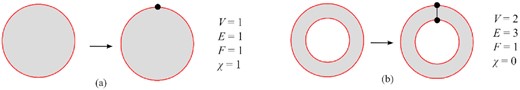
The Euler characteristic of (a) a closed disc; (b) a ring.

The optimum number of elements at a corner

n_{i}

is defined by equation (3) for a corner with an angle

θ_{i}

⁠, and is shown in Fig. 3:

\begin{array}{r} n_{i} = R o u n d (\frac{θ_{i}}{π / 2}) . \end{array}

(3)

Figure 3:

Vertex classification (picture adapted from Fogg et al., 2018).

With the above explanations, it can be easily calculated that the net number of quad mesh singularities for the example in Fig. 1 is

\begin{array}{r} N_{R} = - 4 \times 1 + (2 - 1) \times 5 = + 1, \end{array}

(4)

which means that the number of positive singularities should be one more than that of negative singularities.

Equation (1) gives the net number of quad mesh singularities that are required for the domain. To generate a multiblock decomposition, it is necessary to know the exact number of positive and negative singularities, as well as their location on the surface. The idea of this work is to identify their positions by subdividing the domain into small auxiliary regions and analyse them based on equation (1). When the auxiliary regions are small enough (e.g. compared to the target mesh size), a pair of positive and negative singularities existing in the region can be merged. Therefore, the net number of singularities can be simply treated as the total number of singularities. Two different methods of domain subdivision are proposed. The first method relies on the MA of the domain and the second one relies on offsetting boundary curves inward. Before describing the two methods, two conditions that the subdivision needs to respect are explained.

4. Conditions to Respect

The auxiliary subdivision of a domain can be achieved by introducing either a loop of closed curves or a loop of open curves that connects the boundaries of the domain. It is required that the auxiliary subdivision does not result in a low-quality mesh on the boundary of the domain and does not change the net number of quad mesh singularities after the subdivision as compared to that of the original domain. Two conditions have been set up here to satisfy these requirements and constrain the form of the subdivisions.

Let R be a domain with boundary

\partial R

⁠.

C_{1} \dots C_{n}

is a loop of piecewise curves embedded on R that partitions the R into two subset regions

R_{1}

and

R_{2}

⁠, as shown in Figs 4 and 5.

P_{i}

are the junction points of the curves

C_{1} \dots C_{n}

and

Q_{i}

are the intersection points with the boundary.

α_{1} \dots

α_{n}

are the internal angles at

P_{i} / Q_{i}

R_{1}

(see Fig. 4).

γ_{1} \dots

γ_{n}

are the internal angles of

R_{2}

and are related to

α_{i}

\begin{array}{r} α_{i} + γ_{i} = 2 π . \end{array}

(5)

$Dividing ${\bm{R}}$ using a closed loop of piecewise curves.$

Figure 4:

Dividing $\bm R$ using a closed loop of piecewise curves.

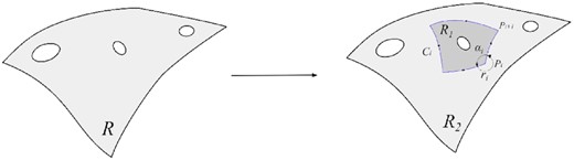
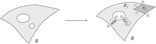
$Dividing ${\bm{R}}$ using an open loop of piecewise curves.$

Figure 5:

Dividing $\bm R$ using an open loop of piecewise curves.

4.1. Condition 1

The first condition is that the subdivision of the domain should respect the classification of the vertices in equation (3). This guarantees that a high-quality mesh is produced on the boundary of the domain at the vertices and satisfies the first requirement.

4.2. Condition 2

The second condition is that α_i should not be the critical values in the vertex classification, i.e. $α_{i} \neq (2 M + 1) π / 4, M = [0, 1, 2, 3] .$ This guarantees that the sum of the net number of mesh singularities of the domains after subdivision is the same as that of the original domain, i.e. $N_{R} = N_{R_{1}} + N_{R_{2}}$ ⁠. In the following, the statement of the second condition will be proved.

Proof

Let us first consider the situation where

C_{1} \dots C_{n}

is a closed loop of curves. Suppose R has m inner loops and

R_{1}

has n inner loops. The Euler characteristics of R and

R_{1}

are

1 - m

and

1 - n

⁠, respectively. The net number of quad mesh singularity of

R_{1}

can be calculated as

\begin{array}{r} N_{R_{1}} = - 4 (1 - n) + \sum (2 - n_{i}^{α}) . \end{array}

(6)

The region

R_{2}

has

m - n

inner loops from R and one inner loop due to the removal of

R_{1}

⁠, so

χ (R_{2}) = 1 - (m - n) - 1

⁠. The net number of quad mesh singularity of

R_{2}

can be calculated as

\begin{array}{r} N_{R_{2}} = - 4 [1 - (m - n) - 1] + \sum (2 - n_{i}^{γ}) + \sum (2 - n_{j}) . \end{array}

(7)

From equations (6) and (7), we have

\begin{array}{r} N_{R_{1}} + N_{R_{2}} = - 4 (1 - m) + \sum (4 - n_{i}^{γ} - n_{i}^{α}) + \sum (2 - n_{j}) . \end{array}

(8)

α_{i} \neq (2 M + 1) π / 4, M = [0, 1, 2, 3]

⁠, combining with equation (5), we have

\begin{array}{r} 4 - n_{i}^{γ} - n_{i}^{α} = 0. \end{array}

(9)

The right-hand side of equation (8) then becomes the net number of quad mesh singularities of R.

Now let us consider the situation where $C_{1} \dots C_{n}$ is an open loop of curves that connects the boundaries of the domain. From condition 1, there need to be two one-element corners at each connection point $Q_{i}$ on the boundary. If the curves connect the outer boundary only, e.g. $C_{1} C_{2}$ in Fig. 5, the statement of condition 2 can be easily proved following a similar process as the above. If the curves connect the outer boundary with an inner boundary, e.g. $C_{3}$ in Fig. 5, or it connects two inner boundaries, e.g. $C_{4}$ in Fig. 5, it will not partition R into two domains. However, the number of inner loops of the new domain will decrease by 1, which means that the Euler characteristic will increase by 1. At the same time, the new domain has four more one-element corners at the connection point on the boundary (e.g. at $Q_{3}$ and $Q_{4}$ ⁠, $Q_{5}$ and $Q_{6}$ ⁠). The effect of these two changes will cancel out when taking them into equation (1). Therefore, the net number of quad mesh singularities does not change before and after the subdivision.

5. The MA-Based Method

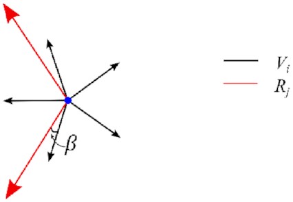
Although it was the inward offset method that was initially suggested in Fogg et al. (2018) as a potential application of equation (1), it was realized later on that the idea can be extended to an MA-based method. The method is more straightforward to understand and therefore will be introduced first. The MA is a skeletal representation of the domain and could be viewed as the locus of the centers of all maximal inscribed spheres. In 2D, the MA is comprised of a set of medial edges and medial vertices, as shown in Fig. 6a. Medial edges connect subsets of the points, where the maximal inscribed circle has two touching points with the boundary. Medial vertices represent the meeting points of medial edges. A point on the MA is equidistant to two or more boundary entities. The line between a point on the MA and its touching point on the boundary is referred to as the medial radius. A medial radius has the property that it is normal to the boundary, except at regions around concave corners. The angle defined by a pair of medial radii is referred to as the medial angle, which is in the range of $(0, 180]$ ⁠. A point along the medial edge has two medial radii and a point on the medial vertex has three or more medial radii. In this work, the MA is generated using the functions in the CADfix software (TranscenData Online).

Figure 6:

(a) Illustration of the MA; (b) four different types of track: The regions filled in green, blue, purple, and yellow represent type-1, type-2, type-3, and type-4 tracks, respectively.

In this method, the auxiliary subdivision is generated using the medial radii at sample points along medial edges. This subdivision strategy is the same as that in Fogg et al. (2016), but the mesh singularity comes straightforwardly as a result of the application of equation (1) instead of the flux analysis.

5.1. Locating quad mesh singularities

The medial radii of any two adjacent sample points on a medial edge or around a medial vertex form a closed region with the boundary, which is referred to as a “track,” as shown in Fig. 6b. Depending on whether a track contains a medial vertex and whether its medial radii connect to a concave corner, a track can be classified as one of the four different types:

Type-1 track: The medial radii of the track do not touch a concave corner and the track does not contain a medial vertex, as highlighted in green in Fig. 6b.
Type-2 track: The medial radii of the track do not touch a concave corner and the track contains a medial vertex, as highlighted in blue in Fig. 6b.
Type-3 track: At least one pair of the medial radii of the track touches a concave corner and the track does not contain a medial vertex, as highlighted in purple in Fig. 6b.
Type-4 track: At least one pair of the medial radii of the track touches a concave corner and the track contains a medial vertex, as highlighted in yellow in Fig. 6b.

If the length of medial edge segments contained in a track is reasonably small (e.g. when compared to the target mesh size), a pair of positive and negative singularities existing in the track can be merged. Therefore, a track’s net number of quad mesh singularities, which can be calculated using equation (1), can be treated as the total number of the quad mesh singularities preferred in the track. The singularity within each track can then be located on the MA, which represents the furthest location from the boundary. In the following, it will show the result of applying equation (1) for each track.

A type-1 track is always six-sided, with two pairs of medial radii and two edges on the boundary, as shown in Fig. 7. It is topologically homeomorphic to a closed disc, which means that its Euler characteristic is 1. The medial radii form four corners at the boundary at right angles. Let S₁ and S₂ be the two sample locations of a track along the medial edge, where the medial radii are created. A vector is created at each of the sample point, with the magnitude being half of the line segment S₁S₂ and the direction being along the bisector of the medial angle, e.g. as V₁ and V₂ shown in Fig. 7a. The sample point, where the created vector points outside of the track, is referred to as S₁ and the other sample point is referred to as S₂. The optimum number of elements of the medial angle (calculated using equation 3) at S₁ is denoted as

n_{out}

and that at S₂ is denoted as

n_{in}

⁠. The net number of quad mesh singularities of the track is then calculated as

\begin{array}{r} N_{R} = - 4 \times 1 + (2 - 1) \times 4 + (2 - n_{out}^{'}) + (2 - n_{in}), \end{array}

(10)

where

n_{out}^{'}

is the number of elements of the track’s internal angle at S₁.

n_{out}

and

n_{out}^{'}

satisfy

\begin{array}{r} n_{out} + n_{out}^{'} = 4, \end{array}

(11)

if the medial angle is not one of the critical values in condition 2 set out in Section 4. Then,

\begin{array}{r} N_{R} = n_{out} - n_{in} . \end{array}

(12)

(a) Two sample points S1 and S2 are created along the medial edge and a vector is created at each of the sample points. (b) We calculate the number of quad mesh singularity in a type-1 track.

Figure 7:

(a) Two sample points S₁ and S₂ are created along the medial edge and a vector is created at each of the sample points. (b) We calculate the number of quad mesh singularity in a type-1 track.

The mesh singularity in a type-1 track is then located at the middle point of the medial edge between the sample points S₁ and S₂.

A type-2 track is 3N-sided, where N is the number of all the sample points of the track (N is also the number of medial radii at the medial vertex in the track). For example, for the type-2 track in Fig. 6b, N has a value of 3 and the track is nine-sided. Vectors are created at the sample points of a type-2 track in a same manner as that of a type-1 track. Let x be the number of the sample points, where the created vector points outside of the track, and

n_{out}

be the optimum number of elements of the medial angle at these sample points. Following the same process as above, the number of quad mesh singularity in a type-2 track can be calculated as

\begin{array}{rcl} N_{R} & = & - 4 + (2 - 1) \times 2 N + \sum_{j = 1}^{N - x} (2 - n_{in}^{j}) + \sum_{i = 1}^{x} (2 - (4 - n_{out}^{i})) \\ = & 4 (N - x - 1) + \sum_{i = 1}^{x} n_{out}^{i} - \sum_{j = 1}^{N - x} n_{in}^{j} . \end{array}

(13)

It can be observed that equation (12) for a type-1 track is a special case of equation (13) for a type-2 track with $N = 2$ and $x = 1$ ⁠. The mesh singularity in a type-2 track is placed at the medial vertex inside the track. Quad mesh singularities identified in type-1 and type-2 tracks are shown in the example in Fig. 8. The green and blue lines represent a medial angle at a sample point with one and two elements, respectively.

Figure 8:

Example 1: quad mesh singularities identified in type-1 and type-2 tracks. The green and blue lines represent a medial angle with one and two elements, respectively.

A type-3 track or a type-4 track has at least one pair of medial radii that connects to a concave corner. Directly using the medial radii connecting a concave corner will violate the expected number of elements at the concave corner. For example, the three-element concave corner in Fig. 6b is partitioned into more than three tracks. To be conformal to the classification of the vertex type and follow the condition 1 in Section 4, an alternative medial radius is required. The method of choosing the alternative medial radii is the same as that in Fogg et al. (2016) but can be understood from a different point of view, which is closely related to the block generation method used in this work. This is explained with reference to the example in Fig. 9. Figure 9a shows a type-3 track and the concave corner that the medial radii connect to. Ideally, a concave corner will be partitioned into several one-element corners, the number of which is based on the vertex classification, e.g. three elements for the example in Fig. 9a. Near the concave corner, the partition lines of the block decomposition should follow the directions of the element edges at the concave corner. The directions of the element can be represented by placing a cross (two perpendicular lines) at the concave corner. The cross is oriented so that it best fits the edges of the concave corner. The direction of the medial radius that connects to a concave corner can then be altered using one of the two directions of the cross, as shown in Fig. 9b and c. The choice of which direction the altered medial radii follow does not affect the number of mesh singularities in the altered track. For example, in Fig. 9c the medial radii on the right-hand side followed a different cross direction from that in Fig. 9b. The fact that the number of singularities is independent of the choice of cross direction can be easily understood since the difference between the altered track in Fig. 9b and c is a rectangle with zero singularities.

Figure 9:

A type-3 track highlighted in purple; (b) and (c): different ways of altering the direction of medial radii of a type-3 track by following different directions of the cross.

The difference between the above two choices is that the altered track in Fig. 9b is classified as a type-1 track, while the one in Fig. 9c is not. To use the same equation as for type-1 or type-2 tracks to calculate the number of mesh singularities, the directions of the medial radii of a type-3 track are altered so that the medial radii on the same side of the MA are nearly parallel; i.e. the difference between the medial angles is close to zero. Therefore, the configuration in Fig. 9b will be used rather than that in Fig. 9c. Following this rule, all type-3 tracks can be altered to a type-1 track. The number of singularities can then be calculated within the altered track and the singularity is located in a similar manner as that of the type-1 track.

Using the same procedure, a type-4 track can be altered to a type-2 track. The singularity in a type-4 track is identified and located in a similar manner as that of the type-2 track. Quad mesh singularities identified in type-3 and type-4 tracks are given in the examples in Fig. 10. These two examples will be referred to as examples 2 and 3 in the following section.

Figure 10:

(a) Example 2: quad mesh singularities identified in a type-3 track; (b) example 3: quad mesh singularities identified in a type-4 track.

5.2. Block generation

After the identification of quad mesh singularities, partition lines are required to decompose the domain into blocks. The MA and the medial radius form a direction field where the medial radius or the altered medial radius (in the following, the medial radius for a concave corner refers to the altered medial radius) represents directions perpendicular to the boundary. A line perpendicular to the medial radius represents a direction following the boundary that the medial radius touches. A segment along the MA represents a direction that best follows both touching boundaries. This information will be used to guide the creation of partition lines. Partition lines are generated in two steps. The starting directions are first determined followed by how they continue until reaching the boundary of the domain. The following known directions can be used as the candidates of the starting directions:

The direction of the medial radius or altered medial radius.
The direction of the bisector of a medial angle with the number of elements being 0 or 2 (this will be the direction of the MA if the medial radii do not connect to a concave corner).
The direction perpendicular to the medial radius.

In an ideal block decomposition, the partition lines at a positive (negative) singularity divide the space into 5 (or 3) equal pieces, as the black lines shown in Fig. 11. This gives an optimum mesh quality around the singularity. The ideal directions are not coincident with the above candidates. Here, the candidate directions that are closest to the ideal directions are selected. To do that, the orientation of the ideal directions at the singularity point needs to be determined first. Let

{V_{i}, i \in Z : i \in [1, N]}

(N = 3

for negative singularity and

N = 5

for positive singularity) be a group of vectors representing the ideal subdivision directions at the singularity, as shown in Fig. 11. The orientation of

{V_{i}}

is determined based on the directions of the medial radius at a singularity point. Let

{R_{j}, j \in Z : j \in [2, M]}

be a group of vectors following the direction of the medial radius.

{β_{j}}

are the smallest angles formed between

{R_{j}}

and

{V_{i}}

⁠.

{V_{i}}

are rotated as a group around the mesh singularity to find a position that minimizes the maximum value in

{β_{j}},

i.e.

\begin{array}{r} m i n i m i z e (m a x {β_{j}}) . \end{array}

$An example of finding the position that $\{ {{\bm{R}}_{\bm{j}}}\} $ best fits to $\{ {{\bm{V}}_{\bm{i}}}\} $ at a positive singularity.$

Figure 11:

An example of finding the position that ${{\bm R}_{\bm j}}$ best fits to ${{\bm V}_{\bm i}}$ at a positive singularity.

A partition line follows the selected starting direction until it reaches a point on the MA or on the medial radius. Its following direction at the new point is determined based on the following rules:

The direction chosen to continue should result in two elements placed at the point.
For a point on a medial radius, it either follows the direction of the medial radius or goes perpendicular to the medial radius.
For a point on the MA, the partition line will either follow the MA until it reaches the medial vertex or go along one of the medial radius directions.
For a point at the medial vertex, it chooses one of the medial radius directions.

The above process continues until the partition line reaches the boundary of the domain or another singularity. It creates a list of points representing a partition line. These points can be used to create a group of straight lines or used as control points to create a Non-uniform rational basis spline (NURBS) curve. Partition lines are also required at concave corners. They start along with the cross directions that are used to determine the altered medial radius and continue following the same rules as those that start from a mesh singularity. The multiblock decomposition of the three examples in Figs 8 and 10 is shown in Fig. 12. The selected three types of candidate directions at the mesh singularity are highlighted in blue, orange, and green, respectively. The purple dashed lines represent a set of straight lines connecting the key points identified during the process. The black solid lines inside each example in Fig. 12b, d, and f represent the smooth NURBS curves created using those key points as control points.

Figure 12:

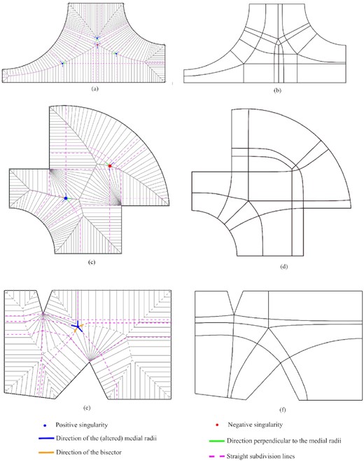
Block decomposition result of the MA-based method: (a), (c), and (e) show the medial radii, singularities, and straight subdivision lines of examples 1, 2, and 3, respectively; (b), (d), and (f) show the decomposition of examples 1, 2, and 3 with smoothed lines, respectively.

6. Offsetting the Boundary Inward Method

The second method relies on creating auxiliary subdivisions by progressively offsetting the boundary of the domain inwards. There are different approaches to achieve the offset patterns (Held, 1998; Choi & Park, 1999; Chen & McMains, 2005; Liu et al., 2007). In this work, the pair-wise offset method is used. The initial concept is to apply equation (1) to each domain produced by an offset and compare the singularities between the two consecutive offset domains. Let

R_{i}

and

R_{i + 1}

be the domain bounded by the

i th

and

(i + 1) th

consecutive offset of the boundary, respectively. Let

R_{i} ∖ R_{i + 1}

be the region between

R_{i}

and

R_{i + 1}

⁠, which is bounded by both the

i th

and

(i + 1) th

offset. The number of mesh singularities that lie in the region

R_{i} ∖ R_{i + 1}

can be calculated as

\begin{array}{rcl} Δ N_{R} & = & N_{R_{i}} - N_{R_{i + 1}} \\ = & 4 (χ_{i + 1} - χ_{i}) + \sum_{j = 1}^{M_{i}} (2 - n_{j}) - \sum_{k = 1}^{M_{i + 1}} (2 - n_{k}), \end{array}

(14)

where

M_{i}

and

M_{i + 1}

are the number of corners of

R_{i}

and

R_{i + 1}

⁠, respectively. An example is given in Fig. 13 where the original domain has a net number of −2. The net number of the

(i + 1) th

offset does not change until it comes to offset

R_{5}

⁠, where the number of singularities for the new domain becomes zero since the two corners are now less than 45 deg. This indicates that two negative singularities are required in the subregion between

R_{4}

and

R_{5}

⁠. While this process identifies the need for singularities, it does not locate them.

$Locate mesh singularities by inward offsetting the boundary: (a) the pattern of the inward offset; (b) singularities identified in the subregion between ${{\bm{R}}_4}$ and ${{\bm{R}}_5}$ (shown as shaded).$

Figure 13:

Locate mesh singularities by inward offsetting the boundary: (a) the pattern of the inward offset; (b) singularities identified in the subregion between ${\bm R}_{4}$ and ${\bm R}_{5}$ (shown as shaded).

In the following, this problem is considered in a different way, which helps us to locate the mesh singularities. During the offset, there exist relations between corners of

R_{i + 1}

and corners of

R_{i}

based on the bounding edges of the corners; e.g. corner

α_{1}^{'}

R_{5}

comes from corner

α_{1}

R_{4}

in Fig. 13. The change in the number of singularities from

R_{5}

R_{4}

is due to the change of the number of elements when the corner

α_{1}

becomes corner

α_{1}^{'}

⁠. Therefore, instead of comparing the net number with respect to the whole domains before and after the offset, it is considered how the change of the corresponding corners will affect the number of mesh singularities. This means that equation (14) can be rewritten as

\begin{array}{r} Δ N_{R} = \sum Δ N^{c}, \end{array}

(15)

where

Δ N^{c}

is the change of singularities related to one group of corresponding corners in

R_{i}

and

R_{i + 1}

⁠.

Δ N^{c}

is calculated as

\begin{array}{r} Δ N^{c} = 4 (χ_{i + 1}^{c} - χ_{i}^{c}) + \sum (2 - n_{i}^{c}) - \sum (2 - n_{i + 1}^{c}), \end{array}

(16)

where

χ_{i + 1}^{c} - χ_{i}^{c}

are the change of Euler characteristic that is related to a group of corresponding corners;

n_{i}^{c}

is a corner in

R_{i}

and

n_{i + 1}^{c}

is a corner in

R_{i + 1}

⁠. For the example in Fig. 13, the corners

α_{1}

and

α_{1}^{'}

form a corresponding group. The Euler characteristic is the same for

R_{4}

and

R_{5}

⁠.

n_{i}^{c}

for

α_{1}

is 1 and

n_{i + 1}^{c}

for

α_{1}^{'}

is 0. Therefore, it is implied that one negative singularity is required between

α_{1}

and

α_{1}^{'}

⁠. Similarly, another negative singularity can be calculated on the right-hand side. This example is simple since the regions before and after the offset have the same Euler characteristic. However, when self-intersection happens during the offset, the Euler characteristic will change after the offset. It is therefore necessary to consider which corner is related to the change of the Euler characteristic. To help with the understanding, a few definitions of offset are first introduced.

The most outside boundary of a domain is referred to as the outer loop. Edges in the outer loop have a positive orientation relative to the surface when they are traversed in a counterclockwise direction when looking towards the plane. Loops of the domain that lie inside the outer loop are inner loops. The inner loop has a positive orientation relative to the face when it is traversed in a clockwise direction when looking towards the plane. During the offset, each boundary curve is offset inwards, and the offset curve takes the same orientation as the curve it is offset from. The offset curves are then extended to meet at a point or trimmed at the self-intersection point. At this stage, the result is comprised of several loops, as shown in Fig. 14. The loops that have orientations following the above definitions are valid offset loops, as shown in red solid in Fig. 14, while the other loops are invalid offset loops, as shown in red dashed in Fig. 14. If an invalid loop connects to one valid loop, it is referred to as a local invalid loop. If it connects to two valid loops, it is referred to as a global invalid loop (GIL). The definitions for invalid loops are consistent to the definitions in Choi and Park (1999) where it is mentioned that an invalid loop is bounded by one tangential circle, which has a radius of the offset distance and makes tangential contact with the boundary and a GIL is bounded by two tangential circles, as shown in grey dashed in Fig. 14.

Figure 14:

An example of pair-wise offset (picture adapted from Choi & Park, 1999).

Figure 15 shows a few representative examples of offsets. The valid offset loops are filled with grey and the GILs are hatched. Figure 15a is an example where no GILs are generated. Figure 15b–d shows that a GIL can be a result of the self-intersection of an outer loop, or between an outer loop and an inner loop, or between inner loops.

Figure 15:

Different cases of offset. The circular points represent the intersection points, and the hashed regions are the GILs: (a) no GILs generated; (b) a GIL generated as a result of the self-intersection of an outer loop; (c) two GILs generated as a result of the intersection between an outer loop and an inner loop; (d) one GIL generated as a result of the intersection between two inner loops.

In the following, it will be proven that the change of Euler characteristic $χ$ after the offset is related to the number of GILs after the offset. More specifically, $χ$ will increase by M if there are M GILs after the offset.

Figure 16:

(a) Original shape; (b) shape after offset without removing the invalid loops; (c) final shape after the removal of the invalid loops.

Proof

Let

R_{i}

be a domain with x inner loops (Fig. 16a). Following the Euler characteristic’s property introduced in Section 3,

\begin{array}{r} χ (R_{i}) = 1 - x . \end{array}

(17)

Let $R_{i}$ be the domain after offset with invalid loops removed (Fig. 16c). $R_{i + 1}^{'}$ is the region combining $R_{i + 1}$ and the GILs, as shown in Fig. 16b. It is first proved that $χ (R_{i}) = χ (R_{i + 1}^{'})$ ⁠. The boundary of $R_{i}$ (or $R_{i + 1}^{'}$ ⁠) divides the infinite plane into three types of regions: $R_{i}$ (or $R_{i + 1}^{'}$ ⁠) itself, the unbounded infinite regions outside $R_{i}$ (or $R_{i + 1}^{'}$ ⁠), and the remaining empty regions inside $R_{i}$ (or $R_{i + 1}^{'}$ ⁠). For $R_{i}$ ⁠, the empty region is bounded by the inner loops. For $R_{i + 1}^{'}$ ⁠, the empty region is the result of the intersection of inner loops with other outer loop or inner loops. The number of the empty loop of $R_{i}$ is same as that of $R_{i + 1}^{'}$ ⁠.

Let

v, e, and f

be the number of vertices, edges, and faces of a valid subdivision of

R_{i}

⁠, respectively.

\begin{array}{r} χ (R_{i}) = v - e + f \end{array}

(18)

Let

v^{'}, e^{'}, and f^{'}

be the number of vertices, edges, and faces of a valid subdivision of

R_{i + 1}^{'}

⁠, respectively.

\begin{array}{r} χ (R_{i + 1}^{^{'}}) = v^{'} - e^{'} + f^{'} \end{array}

(19)

From the planar graph theory,

\begin{array}{r} v - e + r = 2, \end{array}

(20)

where r is the number of regions. Applying this to both

R_{i}

and

R_{i + 1}^{'}

⁠, we get

\begin{array}{r} v - e + \underset{r}{\underset{⏟}{f + x + 1}} = 2 \end{array}

(21)

\begin{array}{r} v^{'} - e^{'} + \underset{r}{\underset{⏟}{f^{'} + x + 1}} = 2. \end{array}

(22)

From the above, we can get that

\begin{array}{r} χ (R_{i}) = χ (R_{i + 1}^{^{'}}) . \end{array}

(23)

Let

v^{''}, e^{''}, and f^{''}

be the number of vertices, edges, and faces of a GIL, respectively. Each GIL will be a simple face with no internal loops. Therefore,

\begin{array}{r} v^{''} - e^{''} + f^{''} = 1. \end{array}

(24)

The GIL has one face, so $f^{'}$ = 1 and $v^{''} = e^{''}$ ⁠.

Let

Σ V

⁠,

Σ E

⁠, and

Σ F

be the sum of vertices, edges, and faces of all GILs, respectively.

\begin{array}{r} \sum V = \sum E, \sum F = M \end{array}

(25)

Then, the Euler characteristic of

R_{i}

\begin{array}{rcl} χ (R_{i}) & = & (v^{'} - (\sum V - 2 M)) - (e^{'} - \sum E) + (f^{'} - M) \\ = & χ (R_{i + 1}) + M . \end{array}

(26)

For example, in Fig. 15b, there are two valid loops after offset and one GIL. So $χ$ goes from 1 to 2 (two faces of $χ = 1$ each). In Fig. 15c, there are two valid loops and two GILs after the offset. The Euler characteristic χ goes from 0 to 2.

6.1. Locating quad mesh singularities

During the offset, the following three types of correspondences between corners $R_{i}$ and $R_{i + 1}$ can be built:

Type 1: A corner of $R_{i + 1}$ comes from one corner in $R_{i}$ and does not connect to a GIL. This means that the parents of its two bounding edges are adjacent before the offset, e.g. $α_{1}$ and $α_{1}^{'}$ in Fig. 15a.
Type 2: A corner of $R_{i + 1}$ comes from multiple corners in $R_{i}$ and does not connect to a GIL. This means that the parents of its two bounding edges are not adjacent before the offset. Also, edges between them disappear after offset, e.g. $β_{1}$ ⁠, $β_{2}$ ⁠, and $β_{1}^{'}$ in Fig. 15a.
Type 3: One or more corners of $R_{i + 1}$ connect to the same GIL and they come from zero or more corners in $R_{i}$ ⁠, e.g. $γ_{1}$ ⁠, $γ_{1}^{'}$ ⁠, and $γ_{2}^{'}$ in Fig. 15b, $γ_{1}^{'}$ and $γ_{2}^{'}$ in both (c) and (d).

For type 1 correspondence, equation (16) becomes

\begin{array}{r} Δ N^{c} = n_{i + 1}^{c} - n_{i}^{c} . \end{array}

(27)

The singularity can be located at the midpoint of the two corners. Examples of negative and positive singularities for this type of correspondences are shown in Fig. 17a and b where the curves before and after offset are shown in solid and dashed lines, respectively. For type 2 correspondence, equation (16) becomes

\begin{array}{r} Δ N^{c} = \sum (2 - n_{i}^{c}) + n_{i + 1}^{c} - 2. \end{array}

(28)

Figure 17:

Examples of singularities during the offset process. The curves before and after offset are shown in solid and dashed lines, respectively. (a) and (b): examples of type 1 correspondence, a singularity located at the midpoint of the two corners; (c) and (d): examples of type 2 correspondence, a singularity placed at the centroid of the multiple corners; (e)–(g): examples of type 3 correspondence, a singularity placed at the centroid of the corners; (h) examples of type 3 correspondence, one singularity will be placed at each corner.

The singularity is placed at the centroid of the multiple corners before and after the offset. Examples are given as shown in Fig. 17c and d. For type 3 correspondence, corners after offset are connected to one GIL and the removal of one GIL causes the Euler characteristic to reduce by 1, so

\begin{array}{r} Δ N^{c} = 4 + \sum (2 - n_{i}^{c}) - \sum (2 - n_{i + 1}^{c}) . \end{array}

(29)

If the index of the singularity is 1 or −1, it will be placed at the centroid of the corners, as shown in Fig. 17e–g. If it is 2 or −2, one singularity will be placed at each corner, as shown in Fig. 17h.

The process of offsetting continues until the shape after offset becomes small; e.g. the length/width of its bounding box is less than the target element size. The singularities of the last shape are calculated using equation (1) and if any exist are located at the center of the shape.

6.2. Block generation

Similar to the MA-based method, the partition lines are generated in two steps. The starting directions are first determined, followed by the extension of the lines. For the singularity identified during the offset process, ideal directions are determined similarly as that of the MA-based method. The difference is that, here, ${R_{j}}$ is formed using the tangent directions of the bounding curves at the corner after the offset. The candidate starting directions are as follows:

The directions perpendicular to bounding curves of the previous offset.
The tangent directions of bounding curves at the corner after offset.
The direction along the bisector or the opposite of the bisector of the corner after offset.

Among the above candidates, those that are closest to the ideal direction are selected. The three types of starting directions at the mesh singularity are highlighted in blue, green, and grey colors, respectively, in Figs 17 and 18. If the singularity is identified within the last offset, the starting directions are selected to be perpendicular to the bounding curves.

Figure 18:

Examples of the subdivision lines and the generated multiblock meshes: (a), (c), and (e) show the offset pattern, singularities, and straight subdivision lines of examples 1, 2, and 3, respectively; (b), (d), and (f) show the decomposition of examples 1, 2, and 3 with smoothed lines, respectively.

The partition line follows the starting directions until it reaches a point on the offset curve. The direction to continue follows the rules below:

The direction chosen to continue should result in two elements placed at the point.
If the point is in the middle of a curve, it either follows the curve or goes perpendicular to the curve.
If it follows the curve and reaches the vertex of a curve, it either follows the other bounding curve at the vertex or goes perpendicular to that curve.
If it follows the direction of the bisector, it continues by connecting to the corner.

The above process continues until the partition line reaches the boundary of the domain or another mesh singularity. It creates a list of points representing a partition line. These points can be used to create a group of straight lines or as the control points to create a NURBS curve. Partition lines are also created from the concave corners. They start by following the directions of a cross that is placed at the concave corner in the same way as in the MA method. It continues by following the above rules for continuing singularities lines from singularities. The block generation results of the three examples in Fig. 12 are shown in Fig. 18. The three types of candidate directions that are selected at the mesh singularity are highlighted in blue, green, and grey, respectively. The straight lines connecting those key points are shown in the purple dashed line in Fig. 18a, c, and e. The smoothed NURBS curves are shown in Fig. 18b, d, and f.

7. Mesh Generation and Smoothing

After the block decomposition, for each block, the mesh can be generated using a mapping algorithm. In this work, the mesh sizing along each block edge is selected to be evenly distributed. The meshing results are shown in Fig. 19. As can be seen, although each block is four-sided and corresponds to a rectangular in the computational space, in the physical space, the opposite edge length of a block can be quite different. This results in uneven distribution of sizing along the geometrical edge of the domain. This nonsmoothness is not preferred in numerical simulations. Here, a Laplacian smoothing is adapted with the mesh on the boundaries adjusted to have an even distribution along the geometry edge.

Figure 19:

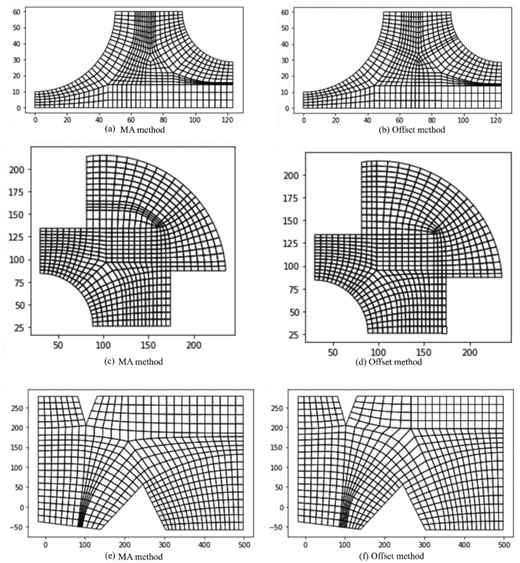
Initial meshing results for the MA method and the offset method; (a), (c), and (e) show MA method of examples 1, 2, and 3, respectively; (b), (d), and (f) show offset method of examples 1, 2, and 3, respectively.

First, the mesh nodes on the boundary are identified. The association between the boundary mesh nodes and the geometry edges is built. This is to determine to which geometrical entities (e.g. vertex/edge) a node lies on and its parametric position on that entity (e.g. t for an edge). Some mesh packages offer this information while others do not. Here, a brute force method is used by taking the mesh node coordinates and querying their relationship with the geometry entities. This process is robust as long as the mesh size is not smaller than the tolerance used in the geometry kernel. Then, a new position of the mesh node is calculated based on the arc length of the edge and the number of mesh elements. From here, a traditional Laplacian smoothing is applied to smooth the mesh. The smoothed mesh result is shown in Figs 20 –22.

Figure 20:

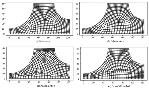
Mesh results from the four different methods for example 1: (a) the MA method; (b) the offset method; (c) Paving method; and (d) the cross-field method.

Figure 21:

Mesh results from the four different methods for example 2: (a) the MA method; (b) the offset method; (c) Paving method; and (d) the cross-field method.

Figure 22:

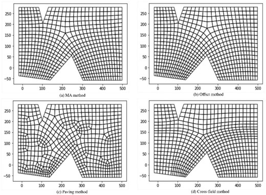
Mesh results from the four different methods for example 3: (a) the MA method; (b) the offset method; (c) Paving method; and (d) the cross-field method.

8. Discussion

This paper describes two methods to locate quad mesh singularities required for a multiblock decomposition. Both are based on the idea of using auxiliary subdivisions of the domain into subdomains and applying equation (1), which calculates the net number of mesh singularities. When the subdomain is small, the change of the net number of mesh singularities is treated as the change of the real number of mesh singularities.

The MA method uses information about the proximity and relative orientations of the model boundary entities that are close to each other. Medial radii are used to subdivide the domain into small tracks and equation (1) is applied to each track to determine the number of singularities. The tracks are classified into four types based on whether they contain a medial vertex and whether they connect to a concave corner. Equations are obtained for the type-1 and type-2 tracks. For type-3 and type-4 tracks, which have at least one medial radius connected to a concave corner, an altered medial radius is used so that the subdivision of the domain respects the optimum number of elements at the boundary. The type-3 tracks are then transformed to type-1 tracks and type-4 tracks are transformed to type-2 tracks by using the altered medial radius. The way the altered medial radius is chosen comes from the consideration that the final decomposition should respect the ideal mesh structure at the concave corner. Singularities are located on the MA, which is the furthest position from the boundary. This means that the irregular nodes are pushed as far away as possible from the boundary. The MA and the medial radius provide a direction field and are used to guide the generation of the subdivisions to achieve a multiblock decomposition. Fogg et al. (2016) used the same method to partition the domain into tracks. Mesh singularities are calculated based on a flux analysis of the track. It is proved in Appendix 1 that the method in Fogg et al. (2016) is equivalent to the method described here. The strategy in Fogg et al. (2016) of decomposition is to create lines that isolate the singularity into separate primitives. Meshes are then created for each primitive. It does not keep the location of the singularity identified in a previous step. The work in this paper uses the information of the MA and media radii to create a decomposition respecting the initial position of the identified singularities.

For the inward offset method, the key point is to determine how the offset layers interact as they advance from the boundary. Instead of comparing the net number with respect to the whole domains before and after the offset, it is considered how the change of the corresponding corners will affect the number of mesh singularities. It is proved that the GIL is related to the change of Euler characteristics. Three types of correspondences between corners before and after offset are built. For each type of correspondence, an equation is derived to calculate the number of mesh singularities. The mesh singularities are placed in the vicinity of the corners. The quad mesh singularity can also appear inside the last offset domain. For the later, the index of singularities is calculated using equation (1) and located in the center of the domain. The curves in the offset pattern provide a direction field and are then used to guide the generation of a multiblock decomposition.

Both methods are applicable to surfaces with computable medial axes and achievable offsets on the surface, which are nonclosed surfaces with boundaries. As pointed out in (D. Systèmes Online), all medial-axis-based methods are most suited to near-planar surfaces or small patches of curved ones. For surface with no boundaries, a possible solution is to first subdivide the surface into a collection of patches using, e.g. geodesic curves.

Both methods presented here are different approaches to an advancing front. So far, four different advancing front methods have been proposed in the literature, namely the paving method, the MA method, the offsetting boundary inward method, and the cross-field method. In the following, the mesh results of the four methods for the three examples used in this work are compared. Paving (Blacker & Stephenson, 1991) is an approach available in most commercial CAE software. In paving, one layer of elements is added to an advancing front from the boundary. Here, the paving method in Siemens NX is used for comparison. The cross-field method selected is the one described in Fogg et al. (2015), which generates boundary aligned crosses and then propagates the cross into the domain in an advancing front manner. The MA method, the offset method, and the cross-field method all generate multiblock decomposition. The mesh sizing of the MA result is used as a reference and the sizing of the other three methods is controlled to be as similar to the MA method as possible along each geometry edge. The overall element numbers of the elements are controlled so that the difference to that of the MA method is within 10 elements. The mesh results can be found in Figs 20 –22.

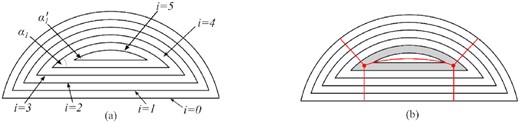
As can be seen, there is a close analogy between the mesh result of the MA approach and that of the offsetting boundary inward approach for both unoptimized meshes in Fig. 19 and the optimized mesh in Figs 20 –22. For a shape without a concave corner, the vertices of the offset pattern will lie on the MA, as shown in Fig. 23a. Tracing the vertices of the offset of a polygon corresponds to the concept of the straight skeleton (Held et al., 2016). For a polygon with no concave corners, the straight skeleton is the same as the MA. However, in cases where concave corners exist, the results will be slightly different due to the concavity, as shown in Fig. 23b and c. For the offsetting method, the concave corner is expanded during the offset process while for the MA method, the concave corner is limited locally. This difference will mean that the location of the mesh singularities may be different when concave corners exist. It can be seen that the locations of the singularities for both methods are very similar for the example in Fig. 12a while they show a slight difference for the example in Fig. 12c. For the result in Fig. 20a and b, if the positive and negative singularity pairs just above each other were below the target element size they could be combined and eliminated. This would give a mesh like the cross-field mesh of Fig. 20d.

Figure 23:

(a) Offset and MA; (b) the straight skeleton; (c) the MA.

For the paving method, a significantly irregular mesh structure is generated. This is because, during the advancing front process of the quad element, only local geometry and topology information is used. The existence of more singularities means that the angle-related mesh quality measurement of the method is normally lower than other methods. The detailed statistics of the three examples in terms of minimum angle measure will be shown in the following section. Unlike the paving method, the offsetting boundary inward method uses the advancing front layers to determine the location of quad mesh singularities. The resulted mesh does not necessarily follow the offset pattern. One advantage of the Paving method is that it can easily adapt to the predefined mesh sizing.

The cross-field method has a smoothing strategy integrated to smooth the cross-field. As a result of this, the locations of the quad mesh singularities are slightly different from the MA and offset methods. Also, positive and negative singularity pairs that are close to each other will be merged during the smoothing, as shown in Fig. 20d. The generated blocks are better than the unsmoothed results from MA and offset method. The cross-field method is based on a conformal mapping, which is angle driven. Sizing is not considered during the mesh generation. This results in uneven distribution of sizing along the geometrical edge of the domain. In fact, for both approaches in this work, a cross-field could be created. For the offsetting boundary inward method, if sample points are placed along the curves of the offset patterns, crosses can be created at the sample points by taking the normal/tangent direction of the curve at the sample point. Similarly, for the MA approach, crosses can be generated along the medial radii and the MA. Therefore, they can be treated in different ways of generating a cross-field.

To have a more detailed comparison of the mesh results, geometric criteria such as the scaled Jacobian, the minimum angle, and the aspect ratio of the elements are measured and the statistic results are shown in Figs 24 –26. The average and minimum/maximum values are calculated as well.

Figure 24:

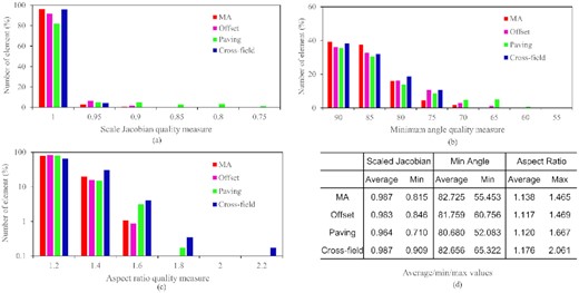
Mesh quality measurement for example 1: (a) the scaled Jacobian quality; (b) the minimum angle quality; (c) the aspect ratio quality; (d) the average/min/max values of the above three quality measures.

Figure 25:

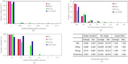
Mesh quality measurement for example 2: (a) the scaled Jacobian quality; (b) the minimum angle quality; (c) the aspect ratio quality; (d) the average/min/max values of the above three quality measures.

Figure 26:

Mesh quality measurement for example 3: (a) the scaled Jacobian quality; (b) the minimum angle quality; (c) the aspect ratio quality; (d) the average/min/max values of the above three quality measures.

For the example in Fig. 24, the MA and cross-field method have the most elements with scaled Jacobian larger than 0.95. The percentage of elements with a scaled Jacobian value larger than 0.95 is 96.32%, 91.8%, 81.91%, and 95.78%, respectively, for the four methods. There are no meshes with a scaled Jacobian below 0.85 for the MA method, offset method, and cross-field method, while 4.86% of the elements are below 0.85 for the paving method. The average scaled Jacobian values are similar for the MA, offset, and cross-field method (∼0.98) and they are slightly higher than that of the paving method (∼0.96). The cross-field method has the largest minimum scaled Jacobian that is 0.909 and the paving method has the smallest value at 0.710. For minimum angle quality, the MA and cross-field method have the most elements with a minimum angle larger than 85 deg. No methods have elements with a minimum angle of less than 60 except the paving method. The MA method and the cross-field method have slightly higher average values than the offset and paving method. The minimum values are 55.453, 60.756, 52.083, and 65.322 deg for the four methods, respectively. For aspect ratio, paving and cross-field method have elements with an aspect ratio >1.8 while the values of the other two methods are <1.8. The cross-field method has the largest average/maximum aspect ratio values.

For the example in Fig. 25, the MA and the offset method have the most elements with scaled Jacobian larger than 0.95. The percentage of elements with a scaled Jacobian value larger than 0.95 is 98.84%, 98.69%, 87.94%, and 96.94%, respectively, for the four methods. There are no meshes with a scaled Jacobian below 0.85 for the MA method, offset method, and cross-field method, while 3.53% of the elements are below 0.85 for the paving method. The average scaled Jacobian values are similar for the MA, offset, and cross-field method (∼0.99) and they are slightly higher than that of the paving method (∼0.97). The cross-field method has the largest minimum scaled Jacobian that is 0.86 and the paving method has the smallest value at 0.667. For minimum angle quality, the MA and offset method have the most elements with a minimum angle larger than 85 deg followed by the cross-field method. No methods have elements with a minimum angle of less than 65 except the paving method. The MA method and the cross-field method have slightly higher average values than the offset and paving method. The minimum values are 63.227, 63.769, 49.213, and 64.670 deg for the four methods, respectively. For aspect ratio, paving and cross-field method have an element with an aspect ratio >1.6 while the values of the other two methods are <1.6. The cross-field method has the largest average aspect ratio value at 1.243 and the paving method has the largest aspect ratio at 1.719.

For the example in Fig. 26, the MA and cross-field method have the most elements with scaled Jacobian larger than 0.95. The percentage of elements with a scaled Jacobian value larger than 0.95 is 95.37%, 94.75%, 84.78%, and 97.72%, respectively, for the four methods. There are no meshes with a scaled Jacobian below 0.85 for the MA method, offset method, and cross-field method, while 3.76% of the elements are below 0.85 for the paving method. The average scaled Jacobian values are similar for the MA, offset, and cross-field method (∼0.99) and they are slightly higher than that of the paving method (∼0.97). The offset and cross-field method has the largest minimum scaled Jacobian that is 0.81 and the paving method has the smallest value at 0.704. For minimum angle quality, the offset method and the cross-field method have the most elements with a minimum angle larger than 85 deg followed by the MA method. No methods have elements with a minimum angle of less than 60 except the paving method. The MA method, the offset method, and the cross-field method have slightly higher average values than the paving method. The minimum values are 59.861, 57.323, 50.380, and 61.749 deg for the four methods, respectively. For aspect ratio, paving and cross-field method have elements with an aspect ratio >1.8 while the values of the other two methods are <1.8. The cross-field method has the largest average aspect ratio value at 1.170 and the largest aspect ratio at 1.753.

From the above-detailed comparison of the three examples, it can be seen that the smoothed result of the MA method, the offset method, and the cross-field result provide mesh with good quality in terms of scaled Jacobian and minimum angle. The ranking varies from example to example, but the differences between them are small. It is noted that the cross-field method tends to give a larger minimum angle compared to the other three methods. However, the aspect ratio value of the cross-field method can be slightly larger. This is because the theory behind this method is based on a conformal mapping between a physical domain and a mapped manifold. This mapping is angle-preserving, but not necessarily length-preserving. It could also result in uneven distribution of mesh sizing along a geometry edge that steps over a few block edges. The results of the methods in this work have improved this.

The proposed methods in this work are based on continuous geometry instead of the discrete meshes. Therefore, it is easier to obtain symmetric decompositions for symmetric domains. Figure 27 shows the multiblock decomposition results of a symmetric example with a circular hole. Figure 27a gives the result from a cross-field-based method. The split lines are forced to stop the first time they meet another split line to give a clear view of the starting parts of the split lines around the circle. Neither the singularities nor the split lines are symmetric. When these nonsymmetric split lines occur around a circle, it could be possible to result in an infinite spiral as shown in Fig. 27b. The same issue is identified by a different cross-field method in Viertel et al. (2019). For the MA method, all the singularities are created lying on the MA. Two of the split lines joining the singularities, L₁ and L₂, are exactly the medial edge, as shown in Fig. 27c. When creating the other two split lines joining the singularities, the dashed red lines are initially created, which will result in degenerate blocks. Using the idea introduced in the following part of the paper, the degenerate blocks can be easily identified and removed, resulting in two single lines L₃ and L₄ joining the singularities. For the offset method, the left-hand/right-hand side two singularities are connected by line L₃/L₄ since the singularities are identified after the same offset has been applied and both singularities are formed by the inward offset of the same boundary edges. The top/bottom two singularities are connected by L₁/L₂ since the singularities are identified after the same offset and the corners related to the two singularities can be traced back to the same GIL.

Figure 27:

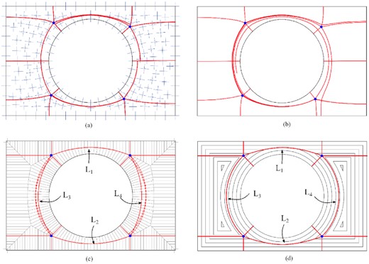
Multiblock decomposition results of a symmetric example with a circular hole: (a) cross-field method with the split line stops when the first time meeting another split line; (b) cross-field method with the split lines shown in (a) continuing which results spiral lines; (c) MA method; (d) offset method.

Both methods in this work are guaranteed to produce singularities that are as far as possible from the boundary. This ensures that mesh distortion close to the boundary is less where high mesh quality is required for a simulation to capture important phenomena (boundary layers, etc.). However, the singularities can be pushed to the boundary in a cross-field method if excessive smoothing is performed, as shown in Fig. 28.

Figure 28:

Excessive smoothing in cross-field method pushes the singularities to the boundary.

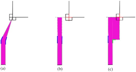
During the process of creating blocks, a partition line should form an angle of approximate 90 deg when it intersects with another partition line. However, if the formed angle is a small angle (less than 45 deg), a degenerate triangular block will be created, as shown in Fig. 29. When this happens, it will be first analysed whether the partition lines can be merged to remove the degenerate blocks. For example, in Fig. 29a, a partition line AE starting from singularity point A intersects with a partition line BD (starting from singularity point B) at point C, creating two degenerate blocks ACD and BEC. Removing the degenerate block means that the length of the edge opposite to the degenerate angle should be changed to zero, e.g. edge AD and edge BE. Point D and point E will then need to be moved to point A and B, respectively. Therefore, a line based on AC and CB will be created to join the two singularities. Similarly, in Fig. 29b, the edge length of AD and BE should be changed to zero, which means that singularity points A and B will be joined together. However, where the removal of the degenerate block is not possible, a partial block will be created. For the example shown in Fig. 29c, two partition lines are created from two three-element concave corners A and B, respectively. The lines AC and BC form a degenerate block, which means that the length of AD and BE should be changed to zero, which is not possible in this case. So, a partial partition line BD is kept with DC removed.

Figure 29:

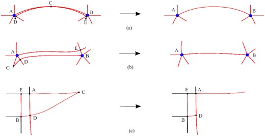
Treatment of degenerate triangular block from the partition lines: (a) and (b): examples of removing the degenerated blocks; (c) an example where the removal of the degenerated block is not possible, and a partial block is created.

More examples of the mesh generated using the methods in the paper are given in Fig. 30.

Figure 30:

More examples of the meshing result of models with holes.

Figure 30:

Continued.

The block decompositions here are achieved based on analysis of angles, which is same as many cross-field methods. It does not consider the sizing constraints on the boundary. One solution to achieve that is to first have a block decomposition using the work here and then introducing pairs of positive and negative mesh singularities in blocks, as suggested in Armstrong et al. (2018). An example is shown in Fig. 31 where one pair of positive and negative mesh singularities is introduced using the method in Armstrong et al. (2018) to improve the sizing of a tapered block. However, some future work needs to be performed to tackle complex cases.

Figure 31:

Introducing an extra pair of mesh singularities to improve the mesh sizing.

In summary, both methods in this paper have provided meshes with a quality comparable to that of the cross-field method. In the future, a systematic study (including FEA and CFD) will be performed to compare the mesh result from the methods in this work and the mesh result from other methods to exploit their numerical performance. The idea presented in this paper to subdivide the domain into small regions will also be explored in 3D for hex mesh generation.

9. Conclusion

This work demonstrates the idea of creating multiblock decomposition based on auxiliary subdivisions. Two methods have been presented in detail. It shows the following:

The strategy of applying an MA-based subdivision to locate quad mesh singularities and generate blocks using the MA and medial radii information.
The strategy of applying an inward offset method to locate the mesh singularity and generate blocks using the offset patterns.
A smoothing strategy to improve the mesh quality and mesh size on the boundary of the domain.

The meshes and the quality of the meshes produced by MA-based subdivision and boundary offsetting were very similar. Both address problems with creating valid block topologies that sometimes occur with cross-field methods. All three methods gave significantly better results than a commercial paving method.

Conflict of interest statement

None declared.

Reference

Ansys

ICEM CFD

[Online]. Available at: https://www.ansys.com/-/media/Ansys/corporate/resourcelibrary/brochure/ansys-icem-cfd-brochure.pdf. [Accessed: 10-Dec-2020]

Armstrong

C. G.

Fogg

H. J.

Tierney

C. M.

Robinson

T. T.

(

2015

Common themes in multi-block structured quad/hex mesh generation

Procedia Engineering

124

–

Armstrong

C. G.

T. S.

Tierney

Robinson

T. T.

(

2018

Multiblock mesh refinement by adding mesh singularities

. In

International Meshing Roundtable

(pp.

189

–

207

.).

Benzley

S. E.

Perry

Merkley

Clark

Sjaardema

(

1995

A comparison of all-hexahedral and all-tetrahedral finite element meshes for elastic and elasto-plastic analysis

. In

Proceedings of the Fourth International Meshing Roundtable

(Vol.

, pp.

179

–

191

.).

Blacker

T. D.

Stephenson

M. B.

(

1991

Paving: A new approach to automated quadrilateral mesh generation

International Journal for Numerical Methods in Engineering

(

811

–

847

Bommes

Zimmer

Kobbelt

(

2009

Mixed-integer quadrangulation

ACM Transactions on Graphics

(

Bunin

(

2008

A continuum theory for unstructured mesh generation in two dimensions

Computer Aided Geometric Design

(

–

Bunin

(

2008

Towards unstructured mesh generation using the inverse Poisson problem

preprint (arXiv:0802.2399)

Campen

Bommes

Kobbelt

(

2015

Quantized global parametrization

ACM Transactions on Graphics

(

–

Chen

McMains

(

2005

Polygon offsetting by computing winding numbers

. In

Volume 2: 31st Design Automation Conference, Parts A and B

(Vol.

2005

, pp.

565

–

575

.).

Choi

B. K.

Park

S. C.

(

1999

A pair-wise offset algorithm for 2D point-sequence curve

Computer-Aided Design

(

735

–

745

Do Carmo

M. P.

(

1976

Differential geometry of curves and surfaces

Prentice-Hall International Inc

Dong

Bremer

P.-T.

Garland

Pascucci

Hart

J. C.

(

2006

Spectral surface quadrangulation

. In

ACM SIGGRAPH 2006 Papers

(pp.

1057

–

1066

.).

D. Systèmes

Abaqus

[Online]. Available at: https://www.3ds.com/products-services/simulia/products/abaqus/ . [Accessed: 01-Dec-2020]

Fogg

H. J.

Armstrong

C. G.

Robinson

T. T.

(

2015

Automatic generation of multiblock decompositions of surfaces

International Journal for Numerical Methods in Engineering

101

(

965

–

991

Fogg

H. J.

Armstrong

C. G.

Robinson

T. T.

(

2016

Enhanced medial-axis-based block-structured meshing in 2-D

Computer-Aided Design

–

101

Fogg

H. J.

Sun

Makem

J. E.

Armstrong

C. G.

Robinson

T. T.

(

2018

Singularities in structured meshes and cross-fields

Computer-Aided Design

105

–

Held

(

1998

Voronoi diagrams and offset curves of curvilinear polygons

Computer-Aided Design

(

287

–

300

Held

Huber

Palfrader

(

2016

Generalized offsetting of planar structures using skeletons

Computer-Aided Design and Applications

(

712

–

721

Huang

Zhang

Liu

Kobbelt

Bao

(

2008

Spectral quadrangulation with orientation and alignment control

ACM Transactions on Graphics (TOG)

(

147

Jezdimirovic

Chemin

Remacle

J. F.

(

2019

Multi-block decomposition and meshing of 2D domain using Ginzburg–Landau PDE

. In

Proceedings of the 28th International Meshing Roundtable

Kälberer

Nieser

Polthier

(

2007

QuadCover-surface parameterization using branched coverings

Computer Graphics Forum

(

375

–

384

Kowalski

Ledoux

Frey

(

2015

Automatic domain partitioning for quadrilateral meshing with line constraints

Engineering with Computers

(

405

–

421

T. S.

Armstrong

C. G.

McKeag

R. M.

(

1997

Quad mesh generation for k-sided faces and hex mesh generation for trivalent polyhedra

Finite Elements in Analysis and Design

(

279

–

301

Lien

J.-M.

Amato

N. M.

(

2006

Approximate convex decomposition of polygons

Computational Geometry

(

1–2

100

–

123

Ling

Huang

Jüttler

Sun

Bao

Wang

(

2014

Spectral quadrangulation with feature curve alignment and element size control

ACM Transactions on Graphics

(

–

Liu

X.-Z.

Yong

J.-H.

Zheng

G.-Q.

Sun

J.-G.

(

2007

An offset algorithm for polyline curves

Computers in Industry

(

240

–

254

Palacios

Zhang

(

2007

Rotational symmetry field design on surfaces

ACM Transactions on Graphics

(

Probst

Mazlum

Radespiel

(

2007

Investigation of computational uncertainties of airfoil flow phenomena close to trailing edges

. In

RTO-Symp. Computational Uncertainty in Military Vehicle Design, RTO-MP-AVT

(Vol.

147

Quadros

W. R.

(

2016

LayTracks3D: A new approach for meshing general solids using medial axis transform

Computer-Aided Design

102

–

117

Rigby

(

2003

Topmaker: A technique for automatic multi-block topology generation using the medial axis

. In

Proceedings of the ASME/JSME Joint Fluids Engineering Conference

(Vol.

, pp.

1991

–

1997

.).

Ruiz-Gironés

Sarrate

(

2010

Generation of structured meshes in multiply connected surfaces using submapping

Advances in Engineering Software

(

379

–

387

Takayama

Panozzo

Sorkine-Hornung

(

2014

Pattern-based quadrangulation for N-sided patches

Computer Graphics Forum

(

177

–

184

Tam

T. K. H.

Armstrong

C. G.

(

1991

2D finite element mesh generation by medial axis subdivision

Advances in Engineering Software and Workstations

(

313

–

324

TranscenData

CADfix

[Online]. Available at: https://www.iti-global.com/cadfix. [Accessed: 01-Dec-2020]

Viertel

Osting

Staten

(

2019

Coarse quad layouts through robust simplification of cross field separatrix partitions

preprint (arXiv:1905.09097)

Xia

Tucker

P. G.

(

2011

Fast equal and biased distance fields for medial axis transform with meshing in mind

Applied Mathematical Modelling

(

5804

–

5819

Xiao

Chen

(

2020

A boundary element-based automatic domain partitioning approach for semi-structured quad mesh generation

Engineering Analysis with Boundary Elements

113

133

–

144

Chen

Deng

(

2015

Two-dimensional domain decomposition based on skeleton computation for parameterization and isogeometric analysis

Computer Methods in Applied Mechanics and Engineering

284

541

–

555

Mourrain

Rabczuk

Bordas

S. P. A.

(

2018

Constructing IGA-suitable planar parameterization from complex CAD boundary by domain partition and global/local optimization

Computer Methods in Applied Mechanics and Engineering

328

175

–

200