


Abstract
A boundary enhancement and Gaussian mixture model (G) optimized synthetic minority oversampling technique (SMOTE) algorithm (BE-G-SMOTE) is proposed to improve diagnostic accuracy under imbalanced bearing fault data conditions. It is designed to solve the problem that the diversity of samples generated by the original SMOTE model is limited, as well as the deep learning model is limited by the size of training samples and processing speed. Firstly, a few bearing fault data are clustered by G to achieve cluster division. Secondly, according to the cluster density distribution function designed in this paper, the weights of different clusters and sample weights to achieve intra-class balance are determined and data quality is improved. Then, to take full advantage of the limited fault data, based on the sensitivity of the support vector machine (SVM) to imbalanced data, the enhanced boundary is established between generated data and the SVM classifier under different penalty factor (PF) values. According to the accuracy, the optimal PF is determined, and fault datasets satisfying diversity are obtained. To improve the classification accuracy, a convolutional neural network with an attention mechanism is built. Finally, analysis using two practical cases shows the effectiveness of the proposed method.
We propose a boundary enhancement and Gaussian mixture model optimized synthetic minority oversampling technique algorithm (i.e., BE-G-SMOTE) combined with convolutional neural network with attention mechanism (CNN-AM) for bearing fault diagnosis.
We establish an optimality bound between the generative model and the support vector machine classifier.
The CNN-AM model is used as the classifier.
The superiority of the method is verified by a self-designed spindle test bench.
List of symbols
- |$\mathrm{G}$|
Gaussian mixture model
- |$\mathrm{BE}$|
Boundary enhancement
- |$\mathrm{CDDF}$|
Cluster density distribution function
- |$\mathrm{PF}$|
Penalty factor
- |$\mathrm{GAN}$|
Generating adversarial network
- |$\mathrm{CNN}$|
Convolutional neural network
- |$\mathrm{AM}$|
Attention mechanism
- |$\mathrm{SMOTE}$|
Synthetic minority oversampling technique
- |$\mathrm{SVM}$|
Support vector machine
- |$\mathrm{ DA}$|
Data augmentation
- |$\mathrm{ GAP}$|
Global average pooling
1. Introduction
Modern production has increasingly demanded the equipment’s intelligence, high efficiency, and astronomical precision. Reliability and health condition monitoring and evaluation of equipment have gradually become hot spots for engineering applications (Raouf et al., 2022). Currently, popular intelligent diagnosis models mainly rely on complete equipment status data and status markers. In engineering practice, it is difficult and costly to obtain fault-type data. The sufficient amount of normal state monitoring data but the insufficient failure data and low-value density will lead to the unbalance of the actual monitoring data of intelligent diagnosis. The data imbalance problem will lead to unsatisfactory efficiency and accuracy of diagnosis, which seriously restricts the application and promotion of intelligent diagnosis theory in engineering. The problem of monitoring data imbalance is a focus in the field of smart diagnostics.
In recent years, data generation models represented by artificial intelligence have gradually emerged, such as generating adversarial network (GAN) models (Goodfellow et al., 2014; Li et al., 2021; Ruan et al., 2021; Wang et al., 2023; Zhang et al., 2020). However, these methods suffer from poor model training stability, time consumption, and parameter redundancy. When the amount of data is extremely imbalanced, it is difficult for deep learning models to learn in-depth information in small-scale data, and the long training time is also an important reason why they are difficult to be applied in engineering (Pan & Yang, 2010; Rohan et al., 2020). Small sample-based classification models such as K nearest neighbors (KNN), random forests, and Bayesian networks also suffer from weak recognition stability and harder to find the optimal kernel parameters, which leads to a lack of classification accuracy (Pan & Yang, 2010; Rohan et al., 2020; Zhong & Liao, 2021). The data generation-based approach can generate sample data containing more information, automatically generated, and after the modeling is completed, it can generate a limitless number of label data, which is more suitable (Zhang et al., 2020) for engineering practice.
Oversampling has widely been used in medicine, recognition, and equipment fault diagnosis because of its fast processing speed and adaptability (Hou et al., 2021; Suh et al., 2019; Zhao et al., 2020). The idea of random oversampling is to copy a few types of data. This method ignores the data distribution and increases the risk of overfitting the classifier after training. Aiming at the above problems, Chawla et al. (2002) proposed the synthetic minority oversampling technique (SMOTE), which effectively solves the overfitting problem by interpolating between minority class samples. Based on this, Han et al. (2005) proposed the borderline-SMOTE algorithm, which avoids blindness in synthesizing new samples by finding the boundary points of a specific class of samples. He et al. (2008) proposed the ADASYN algorithm, which controls the number of new data generated for a few classes of data by the distribution of the overall data. Guan et al. (2021) proposed a data balancing process combining SMOTE and WENN to avoid the interference of overlapping regions between data points of different categories. Xu et al. (2021) achieved improved classification accuracy under imbalanced conditions based on the improved SMOTE algorithm. To make full use of the generation capability of SMOTE under small-scale samples and the power of neural networks, Liu et al. (2021) proposed a data generation method combining SMOTE and CGAN and achieved certain results. But this method needs a long processing time. Most of the current research based on synthetic oversampling improvement algorithms mainly uses the generation of using weight interpolation among limited data points to improve the diversity of generated samples. Still, the amount of information is not increased enough to provide the classifier with classification information beyond the boundary of a few types of data, which makes the generalization ability of the training model general. Secondly, the combination of SMOTE algorithm with models such as GAN is also weak in terms of efficiency. The fault data in practical engineering have diversity, and its distribution domain is not limited to a few data points. Thanks to the above problems, a boundary enhancement and Gaussian mixture model optimized synthetic minority oversampling technique (BE-G-SMOTE) algorithm is proposed. First, based on Gaussian mixture model (G; Huang & Chau, 2008) for clustering a few classes of data samples, cluster density is calculated, and weight sampling is performed to avoid the problem of imbalanced intra-class distribution caused by direct interpolation according to the cluster density distribution function (CDDF) designed in this paper. Second, Support Vector Machine (SVM; Yao Yuan, 2022) have demonstrated excellent performance in the field of unbalanced sample classification. In this paper, the relationship between data generation boundary and SVM classification accuracy is established to avoid the limitation of a few classes with limited data. It achieves the diversity of generated data and enriches classification information on the premise of ensuring classification accuracy.
Based on the fault diagnosis process, a high-performance classifier is required for fault diagnosis after the data samples are balanced. When the sample size is sufficient, the neural network model can perform excellently. In this paper, a convolutional neural network with attention mechanism (CNN-AM; Zhou et al., 2022) model is established to achieve a higher fault diagnosis effect after data balance.
The main contribution of the proposed method in this paper is as follows:
For the problem of intra-class imbalance (Zhang et al., 2020) that exists in a few class samples themselves, G clustering is used, and the CDDF (Wang et al., 2023) achieves weight sampling to solve the intra-class imbalance. To generate higher quality data, based on the excellent performance of SVM in efficiency and performance when dealing with small sample problems, the boundary enhancement (BE) between generated data and SVM classifier is established.
A CNN-AM model for bearing fault diagnosis is built, which effectively improves the fault diagnosis rate. Compared with traditional machine learning algorithms, it has a higher fault diagnosis rate.
The technical route of this paper has obvious advantages over the classical imbalanced data processing method and has a faster processing speed than GANs and better engineering applicability while ensuring diagnostic accuracy, as verified by the experimental design of a fault simulation bench built independently with various indicators.
The rest of this paper is structured as follows: Section 2 presents the relevant theories of this paper. Section 3 describes the methods and specific steps set out in this paper in detail. Section 4 describes two experiments designed in this paper and analyzes them respectively. Finally, Section 5 introduces the conclusions and prospects of this work.
2. Related Work
2.1. SMOTE
SMOTE is a data generation method proposed by Chawla and other scholars to solve the problem of overfitting brought by traditional oversampling algorithms (Chawla et al., 2002). The schematic diagram of SMOTE algorithm is shown in Fig. 1.
Schematic diagram of SMOTE algorithm.
The specific flowchart of the algorithm is as follows:
Initialize the minority sample space |${S}_{\mathrm{min}} = \{ {x}_1,{x}_2,\cdots,{x}_n\} $| and the majority sample space |${S}_{\mathrm{ max}}$|.
The KNN algorithm is used to determine the K samples nearest to the sample |${x}_n$| and record them as |${X}_{nk} = \{ {x}_{n1},{x}_{n2},\cdots,{x}_{nk}\} $|.
- Randomly select m samples from |${X}_{nk}$|, conduct random linear interpolation with sample |${x}_n$|, respectively, and synthesize new samples close to the original data distribution. The formula for its calculation is given in Equation (1):(1)$$\begin{eqnarray} {x}_{\mathrm{ new}} = {x}_n + rand(0,1)\cdot ({x}_n - x_{nk}^m). \end{eqnarray}$$
2.2. Gaussian mixture model
Because clustering algorithms such as K-Mean cannot cluster two classes with the same mean. To solve this problem, this paper uses G for cluster partitioning of minority class-bearing data. G can clearly describe the distribution of the observed data in the overall data. It refers to the distribution and combination of multiple Gaussian kernels. It can be used to describe the distribution of samples in a dataset. G believes that the data are a combination of K Gaussian functions, as shown in Equation (2):
It hides K Gaussian functions, where |${u}_k$| and |${\sigma }_k$| are the parameters of the Kth Gaussian mixing component, and |${\alpha }_k > 0$| is the corresponding “mixing coefficient”. |$\sum\limits_{k = 1}^K {{\alpha }_k} {\rm{ = }}1$|. Taking parameter |$\alpha $| as proportion, the whole data are classified into k categories, each of which conforms to Gauss distribution. Then, based on the maximum likelihood method, |$\alpha $| which determines the proportion of classification and |${u}_k$| and |${\sigma }_k$| which determine the Gauss distribution within the classification are obtained. Finally, the whole data are used to find the corresponding distribution clusters. Iterate to get the best solution by finding a prototype that is close to the data.
2.3. Support vector machine
SVM is a classification model based on statistical learning theory and structural risk minimization principle (Yao Yuan, 2022). The optimal decision function is shown in Equation (3). |${\mathop{\rm sgn}} $| is a sign function. |$K(x,{x}_i)$| uses the |$RBF$| function as shown in Equation (4):
2.4. Convolutional neural networks
The CNN is a deep learning algorithm that imitates the function of the human visual cortex (Ruan et al., 2021). The feature extraction process depends on the convolution kernel, as shown in Equation (5). In the Equation (5), i is the input characteristic diagram serial number; j is the serial number of the output characteristic diagram; |$w_{ji}^l$| is the convolution kernel; |$b_j^l$| is the offset term; and |$r( \bullet )$| is the activation function. The convolution result is processed by the activation function to obtain its corresponding output characteristics. Finally, the classifier outputs the recognition results of the model in the form of category or probability, which converts the extracted features into a probability distribution, and uses the logarithmic probability value to estimate the probability that sample |${x}_i$| belongs to category |${y}_i$|:
3. Method
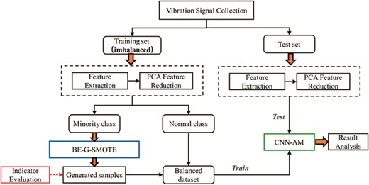
The technical route of this paper as a whole is shown in Fig. 2. A few classes of samples are augmented by BE-G-SMOTE, and then the generated samples are used to train CNN-AM models for fault diagnosis.
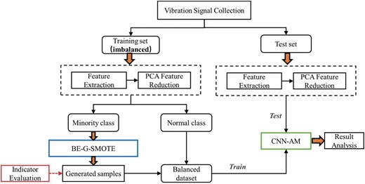
Technology roadmap for this paper.
3.1. BE-G-SMOTE
The data augmentation (DA) framework proposed in this paper is shown in Fig. 3.
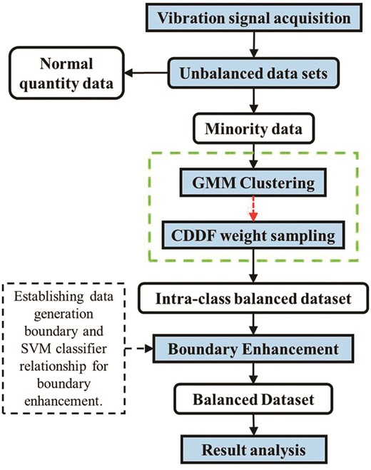
BE-G-SMOTE flowchart.
Specific steps are as follows:
Step 1: A few classes of data in the dataset were clustered using a G, and divided to obtain N clusters: |${C}_I,{C}_2\cdots{C}_N$|.
Step 2: The CDDF based on the hypersphere design is shown in Equation (6). The number of data points contained in a cluster and the number of other contained data points constitute a proportional function of the volume of the hypersphere (Wang et al., 2023). In Equation (6), |$N({C}_l)$| represents the number of data points in a cluster; |$Vol(S({{\rm{d}}}_l))$| represents the volume of the hypersphere formed by the data points; |${{\rm{d}}}_l$| represents the Euclidean distance between the centroid in the cluster and the farthest centroid; and the value of |$D{\rm{en(}}{C}_l{\rm{)}}$| represents the lth density of the data in the cluster:
Step 3: According to step 2, the cluster densities of different clusters can be obtained. The sampling weight |${W}_{}$| in different clusters is determined according to the cluster density of different clusters. The generation weight of the lth cluster |${W}_l$| can be defined as shown in Equation (7). It can sample weights for different clusters. When the sampling weight exceeds the number of neighboring samples, the cluster is repeatedly sampled. After this step, the balanced datasets within the class can be generated:
Step 4: Determine the oversampling multiple N based on the ratio of the balanced dataset within the class to the normal data obtained in step 3. The penalty factor (PF) is added to establish the relationship between the PF and the data boundary generated by the algorithm. The optimal PF is determined according to the iteration condition, and the generated boundary is determined.
The PF is an effective means of transforming the original non-linear constrained problem into a series of unconstrained problems and is widely used in boundary optimization of different models. Applying PF to this method can break the limitation of the original SMOTE algorithm boundary. Based on the accuracy of SVM classification, the PF is continuously modified to obtain the optimal solution of this method.
The specific procedure of step 4 consists of establishing the relationship between the PF and the SVM classifier, and the optimization of the PF.
Step 4a: The relationship between the classification accuracy of the model and training data and test data is defined as |$\mathit{ A{\rm{c}}{{\rm{c}}}}_{\mathrm{ SV{M}}_{\mathrm{ PF}}}{\rm{ = }}{Classification}(\mathrm{ Trai{n}}_{Data}| {\mathrm{ Tes{t}}_{Data}} )$|. The classification accuracy of SVM model is |$\mathit{ A{\rm{c}}{{\rm{c}}}}_{\mathrm{ SV{M}_{PF}}}$|. Assume that the iterative relationship between |$\mathit{ A{\rm{c}}{{\rm{c}}}}_\mathrm{ {SV{M}_{PF}}}$| and |$(PF,{X}_{\mathrm{ PF}})$| is R. When the PF value is different, the generated training data will get different classification results. In this paper, a PF is added to establish the relationship between the data generation boundary and the accuracy of SVM classification as shown in Equation (8).
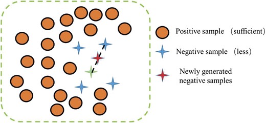
Where, |${\rm{lab1}}$| and |${\rm{lab}}2$| are the offset and scaling factors of the model. |${X}_\mathrm{ S}$| is the training data other than the minority class data. Further, |${X}_\mathrm{ T}$| is the sample used in the BE (model optimization) process. The samples used to test the model performance are not included in the optimization process of the model, they only play a role in the final testing phase, they are put aside in the pre-optimization process of the model, and they do not exist in the optimization formulation.
Step 4b: The optimization search of the relationship |${\rm{R}}$| with the PF is shown in Fig. 4. In the process of finding the best, the accuracy of SVM may be deviated to some extent. Therefore, in each round of this step, we conduct 30 trials and take the highest SVM classification accuracy for retention. The purpose of doing so can well ensure the monotonicity of the merit-seeking curve and reduce the chance. The specific steps are as follows:
Initial PF = 1, the first round is iterated with step a1 = 0.1, and values of SVM classification accuracy are calculated separately. This was stopped when accuracy dropped, PF = PF1d when stopped, at which point accuracy was maximal at PF1d-1.
Initial PF = PF1d-2, iterate according to the step a2=(PF1d-PF1d-2) × 0.1, stop when the accuracy decreases, and obtain the maximum accuracy at PF = PF2d-1. By analogy, enter n rounds of iteration, when ACCNmax-ACCN-1max⇐0.02, the iteration stops. PFbest = PFNd-1.
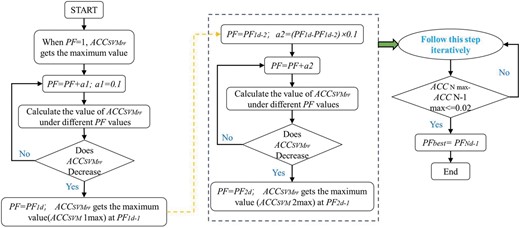
BE process.
Step 5: The balanced dataset is used to train CNN-AM model for fault diagnosis.
3.2. CNN-AM classified model
The AM (Zhou et al., 2022) was a method to filter the features extracted by the self-adapted and weighted filter, and the method to highlight the fault features with important information was widely used. As a new and emerging method of classification, the CNNs had obvious advantages over other machine learning methods. Based on the combination of one-dimensional (1D) CNN and the AM, a CNN-AM classification model was built. The balanced dataset was used to train and sort out the test sets. The model’s parameters were shown in Fig. 5.
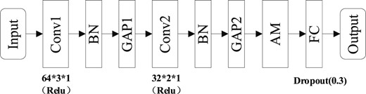
The structure of CNN-AM model.
The fault diagnosis model mainly consists of an input layer, a deep feature extraction layer, an AM layer, and a fully connected layer. The deep feature extraction layer includes a convolutional layer, a batch normalization (BN) layer, and a pooling layer. The convolutional pooling occurs in an alternating manner to perform in-depth feature learning on the input data. Among them, BN is used after convolutional layers since pooling does not change the distribution of elements. After extracting deep features through a series of convolutions pooling, the AM technology is used to filter the information adaptively weighted by the characteristics of different signal segments. At the same time, the filtered features are re-labeled. Finally, the marked feature sequence is sent to the softmax classifier for fault diagnosis.
4. Experimental Verification and Analysis
4.1. Evaluating indicators
The performance of the model is evaluated (Fan et al., 2019) by accuracy and G-mean in this paper. The accuracy (ACC) is shown in Equation (9), and the G-mean is shown in Equation (10):
TN, TI, TO, and TR are the data correctly classified under different categories based on the confusion matrix. FIN is the condition where the classifier considering the inner ring fault is normal. Accuracy is the classification accuracy of the model as a whole. G-mean is the general average of the classification accuracy of a few categories of data and most categories of data, used to evaluate the performance of datasets.
Kullback Leibler (KL) divergence is an indicator used to measure the distribution difference between data (Pan & Yang, 2010). It can reasonably measure the difference between two probability distributions. If the two distributions are closer, the KL divergence is more minor. The definition of KL divergence is shown in Equation (11). In Equation (11), |$p({x}_i)$| is the target distribution; |${x}_i$| is a discrete random variable; and N is the length of the distribution:
4.2. Case 1: data verification of spindle test bench
4.2.1. Experiment introduction
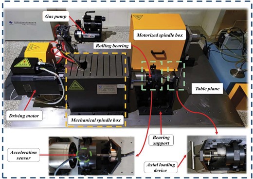
Figure 6 shows the structure of each part of the high-speed spindle test bench. The bearing type is a 7014C rolling bearing with 20 balls. The failure pattern includes normal, outer ring failure, inner ring failure, and rolling element failure. The experimental bearing is shown in Fig. 7.
The structure of CNN-AM model.
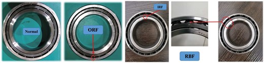
Faulty bearing and its details.
In this experiment, the vibration signals of four types of faults of rolling bearings in running condition were collected, respectively: Normal Condition (NOR), Inner Ring Fault (IRF), Outer Ring Fault (ORF), and Rolling Body Fault (RBF). The specific data situation of the experiment is shown in Table 1. The sampling frequency is 12 KHz, the motor speed is 1200 r/min, the sampling method is interval sampling, the sampling interval is 5 s, the length of each sample is 1 s, and a total of 250 groups are collected.
Experimental setup introduction.
| Bearing type | Rotational speed | Sampling frequency | Fault type | Sample size |
|---|---|---|---|---|
| 7014C | 1200 r/min | 12 KHz | NOR | 250*12 000 |
| IRF | ||||
| ORF | ||||
| RBF |
| Bearing type | Rotational speed | Sampling frequency | Fault type | Sample size |
|---|---|---|---|---|
| 7014C | 1200 r/min | 12 KHz | NOR | 250*12 000 |
| IRF | ||||
| ORF | ||||
| RBF |
4.2.2. Data processing
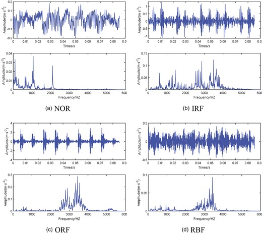
Figure 8 shows the time domain waveforms of the four-fault signals collected in this experiment.
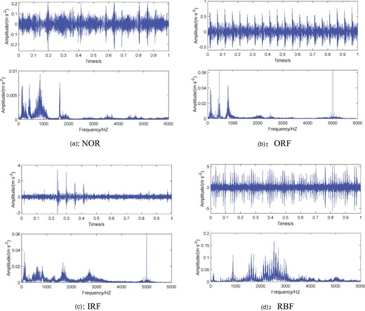
Time domain waveform and frequency spectrum of the collected signal.
To make the data better characterize the fault features, the collected bearing vibration data are feature extracted here. Twenty-six fault features (Yang et al., 2020) are extracted from the original signal. These features are extracted from the time domain and frequency domain of the signal. It includes time domain parameters (e1–e13) and frequency domain features (e14–e26). Specific feature names and calculation formulas are shown in Table 2.
Extracted feature equation.
| Time domain feature | Frequency domain feature | ||
|---|---|---|---|
| |$e1\sim {X}_{|u|} = \frac{1}{N}\sum\limits_{i = 1}^N {|{x}_i|} $| | |$e8 \sim {X}_{if} = \frac{{\mathrm{max}| {{x}_i} |}}{{{X}_{|\mu |}}}$| | |$e14\sim {Y}_{\mathrm{over}} = \sum\limits_{i = 1}^M {{p}_j} $| | |$e21\sim P1 = \sqrt {\frac{{\sum\limits_{k = 0}^{N/1.2} {( {{f}^2*PS[k]} )} }}{P}} $| |
| |$e2\sim {X}_\mu = \frac{1}{N}\sum\limits_{i = 1}^N {{x}_i} $| | |$e9 \sim {X}_{p - p} = {X}_{\mathrm{max}} - {X}_{\mathrm{min}}$| | |$e15\sim {Y}_\mu = \frac{1}{M}\sum\limits_{j = 1}^M {{y}_j} $| | |$e22\sim P2 = \frac{{\sum\limits_{k = 0}^{N/1.2} {( {{f}^2*PS[k]} )} }}{{\sqrt {P*\sum\limits_{k = 0}^{N/1.2} {( {{f}^4*PS[k]} )} } }}$| |
| |$e3 \sim {X}_{ff} = \frac{{\mathrm{max}| {{x}_i} |}}{{{X}_{mss}}}$| | |$e10\sim {X}_{\mathrm{rms}} = \sqrt {\frac{1}{N}\sum\limits_{i = 1}^N {x_i^2} } $| | |$e16\sim {Y}_s = \frac{1}{M}{\sum\limits_{j = 1}^M {\left({\frac{{{y}_j - {Y}_\mu }}{{{Y}_\sigma }}}\right)} }^3$| | |$e23\sim P3 = \frac{{1/M\sum\limits_{k = 0}^{N/1.2} {{{(PS[k] - P/M)}}^3} }}{{\sqrt {{{\left( {1/M\sum\limits_{k = 0}^{N/1.2} {{{(PS[k] - P/M)}}^2} }\right)}}^3} }}$| |
| |$e4 \sim {X}_{cff} = \frac{{\mathrm{max}| {{x}_i} |}}{{{X}_r}}$| | |$e11 \sim {X}_{sf} = \frac{{{X}_{\mathrm{rms}}}}{{{X}_{|\mu |}}}$| | |$e17\sim {Y}_k = \frac{1}{M}{\sum\limits_{j = 1}^M {\left( {\frac{{{y}_j - {Y}_\mu }}{{{Y}_\sigma }}} \right)} }^4$| | |$e24\sim P4 = \frac{{1/M\sum\limits_{k = 0}^{N/1.2} {{{(PS[k] - P/M)}}^4} }}{{{{\left( {1/M\sum\limits_{k = 0}^{N/1.2} {{{(PS[k] - P/M)}}^2} } \right)}}^2}}$| |
| |$e5\sim {X}_k = \frac{1}{N}{\sum\limits_{i = 1}^N {\left( {\frac{{{x}_i - {X}_\mu }}{{{X}_\sigma }}} \right)} }^4$| | |$e12\sim {X}_\sigma = \sqrt {\frac{1}{N}\sum\limits_{i = 1}^N {{{( {{x}_i - {X}_\mu } )}}^2} } $| | |$e18\sim {Y}_{\mathrm{rms}} = \sqrt {\frac{1}{M}\sum\limits_{j = 1}^M {{{( {{y}_j - {Y}_\mu } )}}^2} } $| | |$e25\sim P5 = \sqrt {\frac{{2.56\sum\limits_{k = 0}^{N/1.2} {( {{{(f = P0)}}^2PS[k]} )} }}{N}} $| |
| |$e6\sim {X}_x = \frac{1}{N}{\sum\limits_{i = 1}^N {\left( {\frac{{{x}_i - {X}_\mu }}{{{X}_\sigma }}} \right)} }^3$| | |$e13\sim {X}_r = {( {\frac{1}{N}\sum\limits_{i = 1}^N {\sqrt {|{x}_i|} } } )}^2$| | |$e19\sim {Y}_\sigma = \sqrt {\frac{1}{M}\sum\limits_{j = 1}^M {{{( {{y}_j - {Y}_\mu } )}}^2} } $| | |$e26 \sim P6 = \frac{{\mathop \sum \limits_{k = 0}^{N/1.2.} ( {{{(f - p0)}}^3PS[k]} )}}{{P5}}$| |
| |$e7 \sim {X}_{\sqrt {p - p} } = \sqrt {{X}_{\mathrm{max}} - {X}_{\mathrm{min}}} $| | _ | |$e20\sim {H}_s = - \frac{{\sum\limits_{j = 1}^M {{F}_j\ln {F}_j} }}{{\ln M}}$| | _ |
To improve the model processing speed to reduce redundant features, the principal component analysis (PCA) method was used for feature reduction. After feature extraction of the original data, the size of each fault can be 250 × 26. Firstly, the training set samples are processed by PCA to obtain the PCA feature matrix. The principal components whose cumulative contribution rate of principal components is greater than 95% are taken as the main characteristics (Liu et al., 2014). Then, the different number of fault samples are extracted from them as minority samples for expansion. The distribution of the principal component contribution rate of the training set is shown in Fig. 9. The sum of the cumulative contribution rate of the first four principal components mapped to the PCA space is 97.4%, and the four principal components are reserved to meet the requirements. Then the same data processing operation is performed on the test set samples to verify the reliability of the algorithm.
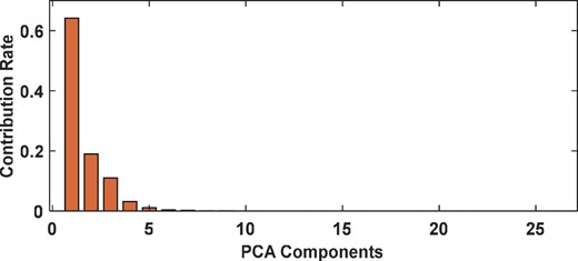
Principal component contribution rate.
To verify the performance of the method in this paper, three test sets with different imbalance rates are designed to verify the effectiveness of the method in this paper. The samples under 160 groups of health were taken as majority class samples, and the samples of 8, 13, and 25 groups of failure types (inner ring, outer ring, and rolling body) were randomly selected as minority class samples with imbalance rates of 5.0%, 8.1%, and 15.6%, respectively. Among the remaining 90 sets of samples, 20 sets of samples for each working condition were taken to participate in model optimization. The remaining 70 groups were used as a test set to test their performance in solving the model to solve the imbalance problem. In actual projects, 10%, 20%, and, 30% do not take place, the randomly determined imbalance rate is designed to better suit the site conditions. The validation dataset of this experimental design is shown in Table 3.
Validate dataset design.
| Dataset number | Fault type | Number of samples in the training set | Number of test set samples | Imbalance rate |
|---|---|---|---|---|
| Dataset A | NOR | 160 | 70 | 5.0% |
| Fault (ORF, IRF, RBF) | 24 (8,8,8) | |||
| Dataset B | NOR | 160 | 8.1% | |
| Fault (ORF, IRF, RBF) | 39 (13,13,13) | |||
| Dataset C | NOR | 160 | 15.6% | |
| Fault (ORF, IRF, RBF) | 75 (25,25,25) |
4.2.3. Analysis of result
Diagnostic accuracy is an essential indicator of the reliability of industrial field devices. The classification accuracy of the three datasets designed in this paper under a more classical classifier is given in Table 4. Each experiment was performed 10 times to take the average value. The analysis shows that the overall accuracy of the classifier is low when the data are out of balance, and the classification accuracy of dataset A is below 50%. When the sample size of a few classes is small, the classification accuracy of 1D CNN is lower than that of the traditional classification model, which indicates that the deep learning method requires a certain amount of data. The classification accuracy shows an overall increasing trend with the increase in the number of samples of fault types. Therefore, it is necessary to perform DA for a few classes of data to improve the diagnosis rate.
The influence of imbalance on classification accuracy.
| Classifier | ||||
|---|---|---|---|---|
| Dataset | KNN | SVM | Random forests | 1D CNN |
| Dataset A | 38.5% | 47.5% | 34.6% | 35.7% |
| Dataset B | 64.2% | 68.5% | 62.5% | 88.2% |
| Dataset C | 76.7% | 80.3% | 78.5% | 91.4% |
| Classifier | ||||
|---|---|---|---|---|
| Dataset | KNN | SVM | Random forests | 1D CNN |
| Dataset A | 38.5% | 47.5% | 34.6% | 35.7% |
| Dataset B | 64.2% | 68.5% | 62.5% | 88.2% |
| Dataset C | 76.7% | 80.3% | 78.5% | 91.4% |
Data augmentation
The RBF data in dataset B are used as a detailed demonstration of the proposed method. Each process in the technical route is displayed through its visualization.
Figure 10 shows 13 groups of RBF data randomly selected in dataset B, which are divided into three clusters after clustering (Han et al., 2005; Son et al., 2020). The cluster density of clusters A, B, and C is 77%, 86%, and 36%, respectively. According to the CDDF, the sampling weights of the three clusters are 3, 2, and 6, respectively. Since cluster C has only two neighboring samples, we repeatedly sampled it within the class with a first weight of 2 and a second weight of 3.
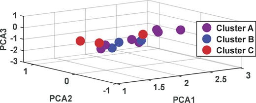
Cluster division of minority class data.
Figure 11 shows the cluster density growth of different clusters after weight sampling. The analysis indicates that the data of a few classes are more balanced in three clusters after G clustering weight sampling, and the method of G clustering and cluster density weight sampling effectively solves the intra-class imbalance problem of a few classes, and the data have better intra-class balance.
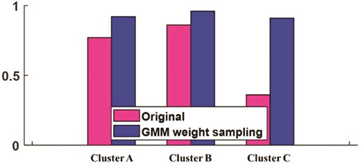
Cluster density growth after G sampling.
Figure 12 shows the variation curves of SVM classification accuracy and G-mean with PF after the fault simulation experimental bench data went through the technical route of this paper. In this experiment, perform 10 times and average, set |${\rm{lab1}}$| = 0.1 and |${\rm{lab}}2$| = 0.7. The analysis shows that the first round of the optimization process stops at PF = 2.4, and the second iteration of the optimization process stops at PF = 2.28, The process of 2.2–2.4 was mapped in its entirety. The classification accuracy reaches the maximum value at PF = 2.26. The SVM classification accuracy is 96.625%, which satisfies the iteration condition. Thus, the final optimization search result of PF = 2.26 is obtained. Figure 13 shows the variation in data volume at different stages.
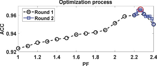
Optimization search with PF.

Changes in the number of samples in different stages (1: original; 2: G weight sampling; and 3: final).
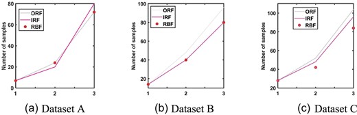
Figure 14 shows the changes in the number of samples in each stage of three different datasets. It is extended by the method proposed in this paper. Other faults in the imbalanced dataset also undergo the above steps to generate data, generating several samples compared to the number of normal samples.
Comparison with other DA methods.
Table 5 shows the accuracy of the three datasets enlarged by this method. According to the analysis, compared with Table 4, we can see that the diagnosis rate increases significantly after data balancing. It can explain the effectiveness of the data amplification method in this paper. The analysis shows that 1D-CNN achieves the highest diagnosis rate of 94.6%, 95.3%, and 97.5% on the three datasets. It can explain the advantage of deep learning approaches when the amount of data is sufficient.
Improved accuracy after DA.
| Classifier | ||||
|---|---|---|---|---|
| Dataset | KNN | SVM | Random forests | 1D CNN |
| Dataset A | 87.5% | 93.2% | 84.6% | 94.6% |
| Dataset B | 90.3% | 96.4% | 88.2% | 95.3% |
| Dataset C | 91.4% | 96.7% | 92.5% | 97.5% |
| Classifier | ||||
|---|---|---|---|---|
| Dataset | KNN | SVM | Random forests | 1D CNN |
| Dataset A | 87.5% | 93.2% | 84.6% | 94.6% |
| Dataset B | 90.3% | 96.4% | 88.2% | 95.3% |
| Dataset C | 91.4% | 96.7% | 92.5% | 97.5% |
Compared with other DA methods
To show the superiority of this method, the index and efficiency of the proposed method were compared with a variety (Wang, 2018) of imbalanced methods.
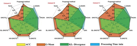
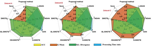
In this test, SVM is used as a classification for all individuals. Each time, they used it 10 times to get an average. As the processing time and KL-dispersion values vary considerably from method to method, they are normalized to “0,1” here. It allows visualizing the performance of the different methods in the radar diagram. The results of the tests are shown in Figure 15.
Comparison with other classification methods.
The results show that the new method has better generation quality and higher classification accuracy and G-means than most of the oversample methods. Compared with the current popular generation network models (GAN, wasserstein GAN (WGAN), and least squares GAN (LSGAN); Luo, 2019). It was known that when the sample size was small (dataset A and B), the GANs were poor in capturing the data rules, and each index was lower than the method and the classical unfair treatment method. When the data scale was large (dataset C), GANs had the advantage of deep learning, with better accuracy of the classification and G-mean value. At the same time, the efficiency of data generation of different models is compared. The analysis shows that this method is faster than GANs. The efficiency of this experiment is about 20 times higher than GANs. In summary, this method achieves higher accuracy and G-means than classical unfair treatment methods and GANs when the size of the minority-type data is small. All the indices were at their highest levels. When the size of the data is fixed, the index of the proposed method is less than 0.5% of the index of GANs, but it is faster to process. All in all, this method had a better generation effect and faster processing speed, which was more suitable for project practice.
Compared with other classification methods
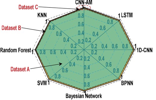
To illustrate the superiority of the CNN-AM model in classification effect, the balanced dataset is generated using the method of this paper, and the classical machine learning algorithm and common neural network model are trained to compare with CNN-AM, respectively. Each experiment was conducted 10 times and the average value was taken. The details are shown in Fig. 15. The results show that CNN-AM has a higher classification effect than other classification models. The data generated using BE-G-SMOTE can give more information to 1D CNN, long short term memory (LSTM), and CNN-AM to take advantage of the deep learning models.
4.3. Case 2: Case Western Reserve University data verification
To prove the effectiveness of the method proposed in this paper, bearing data from Case Western Reserve University (CWRU) in the USA are selected (Li et al., 2021).
4.3.1. Brief introduction of the experiment
The picture of the test bed of CWRU is shown in Figure 16. The bearing type is 6205-RSIEMSKF, the speed is 1797 r/min, the load is 0 N, the fault size is 0.1778 mm, and the sampling frequency is 12 KHz. The data of four working conditions are verified.
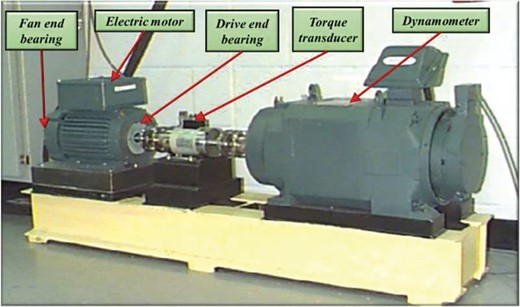
The test bench and fault types of CWRU experiments.
The length of each type of fault data is chosen to be |$117\,760 \times 1$|. Every 1024 points is a sample, and 115 samples are included under each type of fault. Each condition can be divided into 115 groups of samples. Each condition can be divided into 115 sets of samples. In this experiment, 70 sets of each working condition are used as the normal number of samples, and 15 sets of samples are used as the validation set for the boundary finding to participate in the model optimization. The remaining 30 sets of samples are tested to test the model performance. The time domain waveforms and frequency spectra of the four working conditions signals are shown in Figure 17. Figure 18 illustrates the variation in the number of sample size individuals.
Time domain waveform and frequency spectrum of the CWRU data.
In order to verify the effectiveness of the proposed method, three imbalanced datasets with different proportions were also designed in this experiment. The normal failure samples were taken as 70 sets, and the other failure samples were 7, 14, and 28, respectively. Table 6 shows the details of the dataset for the CWRU.
Validate dataset design (CWRU data).
| Dataset number | Fault type | Number of samples in the training set | Number of test set samples | Process optimization participation sample |
|---|---|---|---|---|
| Dataset A | NOR | 70 | 30 | 15 |
| Fault (ORF, IRF, RBF) | (7,7,7) | |||
| Dataset B | NOR | 70 | ||
| Fault (ORF, IRF, RBF) | (14,14,14) | |||
| Dataset C | NOR | 70 | ||
| Fault (ORF, IRF, RBF) | (28,28,28) |
Data augmentation
The CWRU data were also processed by feature extraction and PCA dimensionality reduction. Five principal components were finally retained for each state. The test procedure is consistent with the spindle test and is not repeated here. A small number of class samples from each of the three datasets were sequentially extended using the proposed method to generate equally balanced datasets within the classes.
Changes in the number of samples in different stages (1: original; 2: G weight sampling; and 3: final).
Compared with other DA methods
Figure 19 shows the comparison results between this algorithm and other data generation algorithms. Each test shall be conducted 10 times and the average value shall be taken. The analysis shows that the method proposed in this paper has a better effect on all indicators than most oversampling methods when the data volume is small. Compared with the GANs model, the proposed method has a difference of less than 0.2% in various indexes when the data volume and scale are fixed. Therefore, it has a faster processing speed and is more suitable for engineering practice.
Compared with other DA methods (SVM).
5. Conclusions and Future Works
An improved SMOTE method combined with CNN-AM is proposed to solve the bearing data imbalance problem in this work. We can conclude the following from the analysis:
In the case of limited fault samples, the quality of the samples generated by the proposed data generation method is higher than other methods, and the classification accuracy and G-mean value are the best when comparing the classical imbalance processing methods and GANs. When the fault sample size is sufficient for the GANs model to mine features for data generation, the proposed method does not differ much in classification accuracy, but has faster processing speed.
Building a CNN-AM model suitable for fault classification in this work. Its classification accuracy is higher compared to traditional machine learning and common deep learning methods.
Although the proposed method has achieved some results in the generation of minority data; the generation of vibration signals still has some limitations after feature extraction. In the future, we will focus on the optimization and study of the generation boundary of the oversampling algorithm.
Acknowledgements
This work was supported in part by the National Natural Science Foundation of China under Grant 52065030, and in part by the Key Scientific Research Projects of Yunnan Province under Grant 202202AC080003-3, and in part by the Yunnan Provincial School Education Cooperation Key Project under Grant KKDA202001003. Tao Liu is the corresponding author.
Conflict of interest statement
The authors declared that they have no conflicts of interest to this work.
