Incorporating distribution shifts and spatio-temporal variation when estimating weight-at-age for stock assessments: a case study involving the Bering Sea pollock (Gadus chalcogrammus)

Abstract

Environmental conditions can create spatial and temporal variability in growth and distribution processes, yet contemporary stock assessment methods often do not explicitly address the consequences of these patterns. For example, stock assessments often assume that body weight-at-age (i.e. size) is constant across the stocks’ range, and may thereby miss important spatio-temporal patterns. This is becoming increasingly relevant given climate-driven distributional shifts, because samples for estimating size-at-age can be spatially unbalanced and lead to biases when extrapolating into unsampled areas. Here, we jointly analysed data on the local abundance and size of walleye pollock (Gadus chalcogrammus) in the Bering Sea, to demonstrate a tractable first step in expanding spatially unbalanced size-at-age samples, while incorporating fine-scale spatial and temporal variation for inclusion in stock assessments. The data come from NOAA’s bottom trawl survey data and were evaluated using a multivariate spatio-temporal statistical model. We found extensive variation in size-at-age at fine spatial scales, though specific patterns differed between age classes. In addition to persistent spatial patterns, we also documented year-to-year differences in the spatial patterning of size-at-age. Intra-annual variation in the population-level size-at-age (used to generate the size-at-age matrix in the stock assessment) was largely driven by localized changes in fish size, while shifts in species distribution had a smaller effect. The spatio-temporal size-at-age matrix led to marginal improvement in the stock assessment fit to the survey biomass index. Results from our case study suggest that accounting for spatially unbalanced sampling improved stock assessment consistency. Additionally, it improved our understanding on the dynamics of how local and population-level demographic processes interact. As climate change affects fish distribution and growth, integrating spatiotemporally explicit size-at-age processes with anticipated environmental conditions may improve stock-assessment forecasts used to set annual harvest limits.

spatio-temporal, stock assessment, weight-at-age

Introduction

Fisheries managers depend on stock assessments to make informed decisions about conservation and management measures (Methot, 2009). State-of-the-art methods typically involve fitting an age-structured population dynamics model to evaluate the current and projected status of the resource including biomass and fishing mortality (Hilborn and Walters, 1992). The population dynamics model relies on data from surveys and fisheries to estimate survival patterns and age-specific demographic rates, including growth, mortality, recruitment, and maturation. Key stock characteristics estimated from assessment models are sensitive to changes in these demographic rates (Thorson et al., 2015a). Therefore, the accuracy and precision of the data ultimately impact the value of stock assessments for managers, especially when assumptions such as constant growth rates can be avoided (Methot, 2009; Francis, 2011).

Survey and fishery data on catch rates and composition inevitably have biases and gaps that present challenges to using them in stock assessments (Thorson, 2014; Breivik et al., 2021; Ducharme-Barth et al., 2022). While well-designed fishery-independent surveys attempt to account for known sources of variation with standardized protocols (Gunderson, 1993), there are inevitable disruptions in survey implementation and unobservable sources of variation that make this challenging (Kimura and Somerton, 2007). For instance, sampling intensity may not be equally distributed across a species’ range (Thorson, 2014), there may be aberrant extreme catches (Thorson et al., 2011), and the catchability of survey gear may vary (Kotwicki and Ono, 2018). Resource limitations and weather conditions may contribute to unforeseen gaps in spatial coverage (Adams et al., 2021). In 2020, for instance, many planned surveys were canceled due to COVID-19 restrictions (e.g. NOAA, 2020a,b, c, d). As fish distributions shift due to climate change (Mueter et al., 2011; Pinsky et al., 2020, Rooper et al., 2021), available data may increasingly fail to align with species’ actual ranges (Link et al., 2010; O'Leary et al., 2020) and will exacerbate the challenge of handling biases and gaps in data.

Spatio-temporal models are being used more commonly to address these issues (Maunder and Punt, 2004; Francis, 2011; Maunder et al., 2020; O'Leary et al., 2020; Breivik et al., 2021; Ducharme-Barth et al., 2022). By accounting for persistent spatial differences (i.e. spatial variation) and spatial differences that change over time (i.e. spatio-temporal variation) in the catch rate data, these models can provide better estimates of annual abundance in areas with missing data (e.g. Breivik et al., 2021), extrapolate to unsampled years (e.g. O'Leary et al., 2020), and correct for differences in sampling intensity across the range (e.g. Maunder et al., 2020). Spatio-temporal models have begun to similarly be applied to age composition data (Thorson, 2014; Thorson and Haltuch, 2018; O'Leary et al., 2020). These models provide a way to predict fish density by standardizing catch rates by the area sampled (“area-weighting”) and to predict composition information, such as age and size, by standardizing composition data by the fish density (“density-weighting”) of each location (Thorson et al., 2020). Spatio-temporal models were found to improve prediction and accuracy of abundance estimates over other standardization methods (Thorson et al.,2015b; Gruss et al., 2019; Zhou et al., 2019).

However, spatio-temporal models have rarely been applied to standardizing size-at-age (here defined as weight-at-age), another critical component of assessment models. While there are different methods used to incorporate growth rates in stock assessment models (Helser and Brodziak, 1998; Clark and Hare, 2002; Minte-Vera, 2004; Whitten et al., 2013; Thorson and Minte-Vera, 2016), often an annual size-at-age is derived from size measurements of survey or fishery data in an empirical size-at-age matrix (e.g. Kuriyama et al., 2016; Ianelli et al., 2021). Standardizing data for size-at-age is inherently more complicated than standardizing catch rate for abundance indices because size data results from the interplay between variation in two processes: growth (and resulting size) within different habitats, and the stock abundance in those habitats. First, environmental differences in food availability, temperature, or oxygen may impact local growth rates, resulting in variation in local size-at-age (DeVries and Frie, 1996). Second, fish populations are distributed in space via movement processes that are constrained by physiological limits and dispersal capability. This can lead to spatial mismatches between local food conditions and prey availability, as in the case of the Baltic Sea, where expansion of hypoxic water has concentrated cod into the remaining suitable habitat that lacks their main prey (Casini et al., 2016). The size of cod in this area has consequently drastically declined, at the same time that cod abundance in the same area has increased (Casini et al., 2016). Thus, spatio-temporal variation in both local habitat conditions and population distributions must be considered when standardizing size-at-age. Given these multiple mechanisms, it can be helpful to attribute variation in annual size-at-age to the various processes contributing to them (e.g. Thorson et al., 2017), in this case, spatial and spatio-temporal variation and local size vs. local abundance.

In this study, we used walleye pollock (Gadus chalcogrammus) in the Bering Sea as a data-rich case study in using a spatio-temporal model to incorporate local-scale spatial and temporal variation in size (i.e. weight) and abundance to estimate population-level size-at-age (i.e. a size-at-age matrix for use in a stock assessment). We evaluate the pattern of size over space and time, whether these patterns are persistent or transient (i.e. varying among years), and their implications for the stock assessment. This fishery is particularly relevant to test a spatio-temporal size-at-age model. Bering Sea walleye pollock is the world’s second-largest single-species fishery by catch weight (FAO, 2021) with an average catch of 1.2 million tons since 1979 and first-wholesale value of $1.55 billion in 2019 (Ianelli et al., 2021). The stock is sampled with extensive fishery-independent surveys, providing a rich data set to evaluate spatio-temporal variability in size-at-age. Finally, size-at-age is an important component of the stock assessment because it converts numbers of fish (which forms the basis of the model dynamics) to biomass and catch recommendations. Although the stock assessment is already transitioning to using spatio-temporal models for estimates of a biomass index and age composition (O'Leary et al., 2020), these models have yet to be applied to size-at-age.

Additionally, climate change is predicted to cause significant shifts in the physical and biological regime (Hunt et al., 2008; Whitehouse et al., 2021) that will greatly impact the spatial distribution of walleye pollock (O'Leary et al., 2020). As the pollock range shifts out of the historical survey footprint, spatial gaps in survey data will increase (O'Leary et al., 2020; O'Leary et al., 2022). In addition to incorporating local-scale variation in growth processes and compensating for local abundance, this spatio-temporal model could therefore also enable better predictions of the pollock stock under future climate change by providing a way to extrapolate to unsampled regions as spatial distributions shift. Further research could explore the impact of including covariates and correlation between ages and hauls, as well as short-term forecasting skill. However, we focus here on the first step (showing how model-based estimators compare with existing methods for expanding size-at-age data) and leave these other topics for future research.

It is often difficult to identify the specific environmental features that cause observed variation in fish populations (Thorson et al., 2017; Dambrine et al., 2021). Because of this, here, we constrained our analysis to quantifying latent spatial and spatio-temporal variation and to retrospective size-at-age data to determine the best analysis protocols, to establish an operating model framework, and to ensure that it could replicate existing estimators and be applied in the stock assessment before delving into covariates and forecasts. Here, we focus on an initial assessment of the pattern of spatial and temporal variation in size-at-age in the Bering Sea pollock, the demographic processes contributing to this variation, and how this model impacts outcomes of the stock assessment.

We seek to answer the following questions:

How does size-at-age vary spatially and temporally, both locally and at the aggregated population-level (i.e. the size-at-age matrix used in the stock assessment)?
How do local spatial and spatio-temporal variation impact the size-at-age matrix?
How does local variation in size vs. abundance contribute to the size-at-age matrix?
How does our spatio-temporal model of the size-at-age matrix affect the stock assessment predictions of population biomass compared to a simple empirical estimate?

To do so, we develop a spatio-temporal model for size-at-age and fish density, and use this to calculate the population-level size-at-age, i.e. the “size-at-age matrix”, that is used as input within many stock-assessment models worldwide (e.g. Kuriyama et al., 2016). We then evaluate the drivers within the model and explore its inclusion in a stock assessment compared to a simple empirical estimate.

Methods

We aimed to estimate annual time series of population size-at-age (i.e. a size-at-age matrix) for the Bering Sea walleye pollock that incorporated local spatial variability in size-at-age, while also compensating for shifts in the relative density of areas with small and large fish. This required an estimate of two response variables—average size and fish density—for each age class for each year in distinct locations across the Bering Sea. Then, to aggregate the local size-at-age at each location up to the population level, we area-expanded fish density to abundance and weighted the size-at-age at each location by the local abundance-at-age in that year to calculate the population-level “size-at-age matrix”. We therefore sought to estimate density and size in a joint model. To accommodate estimating both response variables in a single-joint model, we used a flexible model structure (a Poisson-link delta approach to a generalized linear mixed model) that predicts density-at-age |${n_{a,y,g\;}}$| and size-at-age |${w_{a,y,g}}$| for each year y and age a for distinct locations in space g, while accounting for annual effects and spatial fields that cover spatially and temporally dynamic latent variables. We then evaluated how these estimates might affect key outcomes in a stock assessment model.

Data compilation

The model was fitted to data collected from the NOAA Groundfish Bottom Trawl Survey from 1982 to 2019. Estimating size-at-age relied on the specimen age a_i (years), weight v_i (grams), and length l_i (millimeters) measurements that are subsampled as part of hauls in the survey. Surveys were not conducted in 2020, and completed survey data from 2021 were not available at the time of this study. Surveys from 1984 to 1998 did not measure individual fish weights because motion-compensating scales were not widely available at that time (e.g. Wilson and Armestead, 1991; Walters, 1997; Nebenzahl and Goddard, 2000). After 1991, specimen weights were sampled sporadically, and were consistently measured from 1999 onwards. For 1984–1999, weight was estimated from measured lengths using sex-specific weight–length conversion parameters (Ianelli et al., 2021). Individual fish from the northern Bering Sea survey were not aged by the time this study was completed. Additionally, there were no specimen data available for age-14 in 2018 and age-15+ in 1986 and 2019. The density-at-age data that we used are the age-stratified, density-dependence-corrected catch-per-unit-effort (CPUE) per haul (numbers of fish hectare⁻¹) c_i [see Kotwicki et al. (2014) for details]. Figure 1 shows the spatial distribution of survey data for a subset of years, and the general geographic extent of CPUE and specimen weight or length data are similar. See Supplementary Figure 1 for full time series of locations of specimen weight and length data and Supplementary Figure 2 for CPUE data.

Figure 1.

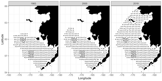
Bottom trawl survey locations in the Bering Sea for subset of years to show extent of survey over time.

Open in new tab Download slide

Model structure

Average local size |${w_{g,a,y}}$| for each year y and age a for distinct locations in space g was estimated using a log-linked generalized linear mixed model. The model includes a single linear predictor that contains terms for temporal variation |$\beta $|⁠, spatial variation |$\omega $|⁠, and spatio-temporal variation |$\varepsilon $|⁠.

$$\begin{eqnarray} && \log \left( {{w_{{g_i},{a_i},{y_i}}}} \right)\\&&\quad = \underbrace {{\beta _{\;\;{a_i},{y_i}}}}_{Temporal\;variation} + \underbrace {{\omega _{{g_i},{a_i}}}}_{Spatial\;variation} + \underbrace {{\varepsilon _{{g_i},{a_i},{y_i}}}}_{Spatio - temporal\;variation}. \end{eqnarray}$$

(1)

Temporal variation was estimated as a fixed effect for each age a and year y, and represents a fixed intercept for each age and year. Spatial and spatio-temporal variation were estimated as Gaussian random effects with mean 0 and were assumed to follow a multivariate normal distribution with covariance matrices |$\sigma _{\rm{\omega }}^2{{\bf{R}}_{\bf{\omega }}}$| and |$\sigma _\varepsilon ^2{{\bf{R}}_\varepsilon }$|⁠. Covariance matrices include the correlation between locations, calculated using a Matérn function in the correlation matrices |${{\bf{R}}_{\bf{\omega }}}$| and |${{\bf{R}}_\varepsilon }$|⁠, which are governed by a shared decorrelation rate |${\rm{\kappa }}$| (i.e. the distance that locations are uncorrelated), and the estimated marginal variances |${\sigma _\omega }$| and |${\sigma _\varepsilon }.\;$| Spatio-temporal variation also follows an auto-regressive process, governed by the autocorrelation parameter |${\rho _\varepsilon }$|⁠.

$$\begin{eqnarray} {{\bf{\omega }}_a}\sim{\rm{MVN}}\left( {{\bf 0},\sigma _{\rm{\omega }}^2{{\bf{R}}_{\bf{\omega }}}} \right), \end{eqnarray}$$

(2)

$$\begin{eqnarray} {{\bf{\varepsilon }}_{a,y}}\sim\{ \begin{array}{@{}*{2}{c}@{}} {{\rm{MVN}}\left( {{\bf 0},\sigma _\varepsilon ^2{{\bf{R}}_\varepsilon }} \right)}&{{\rm{if\;}}t\; = \;1}\\ {{\rm{MVN}}\left( {{\rho _\varepsilon }{{\bf{\varepsilon }}_{a,y - 1}},\sigma _\varepsilon ^2{{\bf{R}}_\varepsilon }} \right)}&{{\rm{if\;}}t > 1}.\end{array} \end{eqnarray}$$

(3)

The measured size |${v_i}$| is assumed to follow a lognormal distribution, with log-mean |$\log ( {{w_{{g_i},{a_i},{y_i}}}} )$| and log-variance |$\sigma _{\rm{v}}^2$|⁠.

$$\begin{eqnarray} \Pr \left( {V\; = \;{v_i}} \right) = \;{\rm{lognormal}}({v_i}|\log \left( {{w_{{g_i},{a_i},{y_i}}}} \right),\;\sigma _{\rm{v}}^2). \end{eqnarray}$$

(4)

In order to weight the local size estimates from this size-at-age model by the local abundance at each location in each year, we additionally needed a similar spatio-temporal model of density-at-age |${n_{g,a,y\;}}$| for each year y and age a for distinct locations in space g. However, catch rates contain many zeroes for certain ages in certain years (Martin et al., 2005). To accommodate for zero-inflation in the model of abundance, we used a Poisson-link delta approach to a generalized linear mixed model (Thorson, 2018). This approach calculates the probability of encounter |${r_{1,i}}$| from a Poisson distribution, whose rate parameters are governed by linear predictor |${p_{1,i}}$| (i.e. a complementary log–log link function), and the density if encountered |${r_{2,i}}$| from the Poisson distribution modeled as |${p_{1,i}}$|⁠, and a gamma-distributed multiplier of counts, whose mean and variance are determined by a linear predictor |${p_{2,i}}.$| Thus, the encounter rate |${r_{1,i}}$| and density if encountered |${r_{2,i}}$| equal:

$$\begin{eqnarray} {r_{1,i}} = 1 - {e^{ - {e^{{p_{1,i}}\;}}}}, \end{eqnarray}$$

(5)

$$\begin{eqnarray} {r_{2,i}} = \frac{{\;{e^{{p_{1,i}}}}}}{{{r_{1,i}}}} \times {e^{{p_{2,i}}}}. \end{eqnarray}$$

(6)

Final estimated density |${n_{i\;}}$| is then the product of |${r_{1,i}}$| and |${r_{2,i}}$|⁠, such that |$\log ( {{n_i}} ) = {p_{1,i}} + {p_{2,i}}$|⁠.

Because both linear predictors are included in the calculation of positive catch rates |${r_{2,i}}$|⁠, including the three variation terms in the first linear predictor includes them in both |${r_{1,i}}$| and |${r_{2,i}}$|⁠. To simplify the model for computational efficiency, temporal, spatial, and spatio-temporal variation are included in the first linear predictor, |${p_{1,i}}$| , while only temporal variation was included in the second linear predictor. When using the Poisson-link delta model, the variance associated with the second linear predictor is typically small, and we can assume that excluding the terms in the second linear predictor will have negligible impacts on the model estimates (see Thorson 2018).

$$\begin{eqnarray} {p_{1,i}} = \underbrace {{\beta _{{\rm{\;\;}}1,{a_i},{y_i}}}}_{Temporal{\rm{\;}}variation} + \underbrace {{\omega _{{g_i},{a_i}}}}_{Spatial{\rm{\;}}variation} + \underbrace {{\varepsilon _{{g_i},{a_i},{y_i}}}}_{Spatio - temporal{\rm{\;}}variation}, \end{eqnarray}$$

(7)

$$\begin{eqnarray} {p_{2,i}} = \underbrace {{\beta _{{\rm{\;\;}}2,{a_i},{y_i}}}}_{Temporal{\rm{\;}}variation}. \end{eqnarray}$$

(8)

The probability of not encountering an age-class in a given sample [i.e. Pr(⁠|${C_i}$|=0)] equals |$1 - {r_{1,i}}$|⁠, and the positive catch rates |${C_i}$| > 0 were assumed to follow a gamma distribution, governed by shape parameter |$k$| and scale parameter |$\theta $|⁠, with mean |${r_{2,i}}$| and coefficient of variation (CV) |${\sigma _r}$|⁠, where |$k = \frac{1}{{\sigma _r^2}}$| and |$\theta $|=|${r_{2,i}}\; \times \;\sigma _r^2$|⁠.

$$\begin{eqnarray} \Pr \left( {C\; = {\rm{\;}}{c_i}} \right) = \Big\{ \begin{array}{@{}*{2}{c}@{}} {1 - {r_{1,i}}}&{{\rm{if\;}}c = 0}\\ {{r_{1,i}} \times {\rm{\;gamma}}\{ c|{r_{2,i}},\sigma _r^2\} }&{{\rm{if\;}}c > 0}. \end{array} \end{eqnarray}$$

(9)

We implemented this joint spatio-temporal size- and density-at-age model using the R package VAST version 3.8.2 (Thorson, 2019). This package allows the flexibility to do a multivariate spatio-temporal model, essentially treating each size- and density-at-age as a different response variable (i.e. category). Each category is specified with its probability distributions and link function, and separate spatial (i.e. omega term) and spatio-temporal (i.e. epsilon term) variation are estimated for each size- and density-at-age. Spatial and spatio-temporal terms are not correlated across ages. This package also allowed the flexibility to estimate both size- and density-at-age by using a Poisson-link delta approach that estimated density-at-age as in Equations (5) to (9), but essentially fixed the encounter probability for size-at-ages at 1 (i.e. 100% encountered) to ultimately estimate size-at-age by a single linear predictor. For additional details on how this joint model was coded in VAST, see Supplementary Methods Section 2. Additional information on code and documentation of the VAST package is available at https://github.com/James-Thorson-NOAA/VAST.

Ultimately, the model extrapolated size and abundance by predicting density-at-age |${n_{g,a,y\;}}$| and size-at-age |${w_{g,a,y}}$| for each year y and age a for distinct locations in space g. The model estimated spatial and spatio-temporal effects across 500 points (i.e. termed “knots” in VAST) that were uniformly distributed across the Bering Sea and used bilinear interpolation to cover the entire geographic extent of the model (in this case, the Bering Sea) between these points with 51769 distinct locations (i.e. grid cells g). We established that 500 knots were sufficient by qualitatively comparing model predictions over a range of knots. Density- and size-at-age were estimated for each of the years 1982–2019 at each of these 51769 locations spanning the region. Approximating the multivariate normal distribution was accomplished using the SPDE method (Lindgren et al., 2011), and the matrices involved were calculated using R-INLA (Lindgren and Rue, 2015). See Supplementary Figure 3 for the map of the SPDE mesh, Supplementary Table 2 for estimated model parameters, and Table 1 for a summary of definitions of variable names and symbols.

Table 1.

Open in new tab

Variable names and symbols used in data processing and model outputs.

Name	Symbol	Units
*Indices*
Specimen (data)	i	–
Haul (data)	h	–
Age (data and model)	a	Year
Year (data and model)	y	–
Grid cell (model)	g	–
*Data inputs*
Fish specimen size (weight)	v_i	Grams
Fish specimen fork length	l_i	Millimeters
Catch rate (density-corrected CPUE)	c_i	Number of fish hectare⁻¹
Model components
Temporal variation	\|$\beta $\|	–
Spatial variation	\|$\omega $\|	–
Spatio-temporal variation	\|$\varepsilon $\|	–
Linear predictor	\|$p$\|	–
Encounter probability	\|${r_1}$\|	–
Density if encountered	\|${r_2}$\|	–
Autocorrelation for spatio-temporal variation	\|${\rho _\varepsilon }$\|	–
Spatial correlation matrix for spatio-temporal variation	\|${{\bf{R}}_\varepsilon }$\|	–
Spatial correlation matrix for spatio-temporal variation	\|${{\bf{R}}_{\bf{\omega }}}$\|	–
Shape parameter of gamma distribution	\|$k$\|	–
Scale parameter of gamma distribution	\|$\theta $\|	–
*Model outputs*
Fish density (i.e. density)	n	Number of fish hectare⁻¹ (or km⁻²)
Abundance	\|$\hat n$\|	Number of fish
Size (i.e. weight)	w	Grams
Abundance-weighted size	\|$\hat w$\|	Kilograms
Area	A	Kilometer²

Name	Symbol	Units
*Indices*
Specimen (data)	i	–
Haul (data)	h	–
Age (data and model)	a	Year
Year (data and model)	y	–
Grid cell (model)	g	–
*Data inputs*
Fish specimen size (weight)	v_i	Grams
Fish specimen fork length	l_i	Millimeters
Catch rate (density-corrected CPUE)	c_i	Number of fish hectare⁻¹
Model components
Temporal variation	\|$\beta $\|	–
Spatial variation	\|$\omega $\|	–
Spatio-temporal variation	\|$\varepsilon $\|	–
Linear predictor	\|$p$\|	–
Encounter probability	\|${r_1}$\|	–
Density if encountered	\|${r_2}$\|	–
Autocorrelation for spatio-temporal variation	\|${\rho _\varepsilon }$\|	–
Spatial correlation matrix for spatio-temporal variation	\|${{\bf{R}}_\varepsilon }$\|	–
Spatial correlation matrix for spatio-temporal variation	\|${{\bf{R}}_{\bf{\omega }}}$\|	–
Shape parameter of gamma distribution	\|$k$\|	–
Scale parameter of gamma distribution	\|$\theta $\|	–
*Model outputs*
Fish density (i.e. density)	n	Number of fish hectare⁻¹ (or km⁻²)
Abundance	\|$\hat n$\|	Number of fish
Size (i.e. weight)	w	Grams
Abundance-weighted size	\|$\hat w$\|	Kilograms
Area	A	Kilometer²

Table 1.

Open in new tab

Variable names and symbols used in data processing and model outputs.

Name	Symbol	Units
*Indices*
Specimen (data)	i	–
Haul (data)	h	–
Age (data and model)	a	Year
Year (data and model)	y	–
Grid cell (model)	g	–
*Data inputs*
Fish specimen size (weight)	v_i	Grams
Fish specimen fork length	l_i	Millimeters
Catch rate (density-corrected CPUE)	c_i	Number of fish hectare⁻¹
Model components
Temporal variation	\|$\beta $\|	–
Spatial variation	\|$\omega $\|	–
Spatio-temporal variation	\|$\varepsilon $\|	–
Linear predictor	\|$p$\|	–
Encounter probability	\|${r_1}$\|	–
Density if encountered	\|${r_2}$\|	–
Autocorrelation for spatio-temporal variation	\|${\rho _\varepsilon }$\|	–
Spatial correlation matrix for spatio-temporal variation	\|${{\bf{R}}_\varepsilon }$\|	–
Spatial correlation matrix for spatio-temporal variation	\|${{\bf{R}}_{\bf{\omega }}}$\|	–
Shape parameter of gamma distribution	\|$k$\|	–
Scale parameter of gamma distribution	\|$\theta $\|	–
*Model outputs*
Fish density (i.e. density)	n	Number of fish hectare⁻¹ (or km⁻²)
Abundance	\|$\hat n$\|	Number of fish
Size (i.e. weight)	w	Grams
Abundance-weighted size	\|$\hat w$\|	Kilograms
Area	A	Kilometer²

Name	Symbol	Units
*Indices*
Specimen (data)	i	–
Haul (data)	h	–
Age (data and model)	a	Year
Year (data and model)	y	–
Grid cell (model)	g	–
*Data inputs*
Fish specimen size (weight)	v_i	Grams
Fish specimen fork length	l_i	Millimeters
Catch rate (density-corrected CPUE)	c_i	Number of fish hectare⁻¹
Model components
Temporal variation	\|$\beta $\|	–
Spatial variation	\|$\omega $\|	–
Spatio-temporal variation	\|$\varepsilon $\|	–
Linear predictor	\|$p$\|	–
Encounter probability	\|${r_1}$\|	–
Density if encountered	\|${r_2}$\|	–
Autocorrelation for spatio-temporal variation	\|${\rho _\varepsilon }$\|	–
Spatial correlation matrix for spatio-temporal variation	\|${{\bf{R}}_\varepsilon }$\|	–
Spatial correlation matrix for spatio-temporal variation	\|${{\bf{R}}_{\bf{\omega }}}$\|	–
Shape parameter of gamma distribution	\|$k$\|	–
Scale parameter of gamma distribution	\|$\theta $\|	–
*Model outputs*
Fish density (i.e. density)	n	Number of fish hectare⁻¹ (or km⁻²)
Abundance	\|$\hat n$\|	Number of fish
Size (i.e. weight)	w	Grams
Abundance-weighted size	\|$\hat w$\|	Kilograms
Area	A	Kilometer²

Annual population size-at-age

From these 51769 local estimates of size-at-age for each year, we wanted an average annual population-level size-at-age (i.e. “size-at-age matrix”) that incorporated local variation in size and compensated for the local abundance. This is because the stock assessment model requires a size-at-age matrix with dimensions age × year. To that end, for each year, we calculated a weighted average of size-at-age, weighted by the local abundance. First, the modelled density |${n_{g,a,y\;}}$| per age a, year y, and grid cell g (in number of fish hectare⁻¹) was expanded by the area |${A_g}$| of the grid cell (in kilometers²) to calculate area-expanded abundance |${\hat n_{g,a,y}}$| (with units numbers of fish) using Equation (10). |${\hat n_{g,a,y}}$| was then summed across all grids per year and per age to calculate the annual, population-level area-expanded abundance |${\hat n_{a,y}}$|⁠.

$$\begin{eqnarray} {\hat n_{a,y}} = {\rm{\;}}\mathop \sum \nolimits_{g\; = {\rm{\;}}1}^G \left( {{n_{g,a,y{\rm{\;}}}} \times {A_g}} \right). \end{eqnarray}$$

(10)

Second, a weighted average of size for each age class and year, |${\hat w_{a,y}},$| was calculated by weighting size-at-age |${w_{a,y,g}}$| by the abundance associated with this extrapolation point |${n_{g,a,y\;}} \times {A_g}$|⁠.

$$\begin{eqnarray} {\hat w_{a,y}} = \mathop \sum \nolimits_{g = 1}^g [{w_{g,a,y}} \times {\rm{\;}}\left( {\frac{{{n_{g,a,y{\rm{\;}}}} \times {A_g}}}{{{{\hat n}_{a,y}}}}{\rm{\;}}} \right)]. \end{eqnarray}$$

(11)

Question 1: spatial and temporal patterns of size-at-age

We descriptively evaluated spatial and temporal patterns in the model predictions of size and abundance at the local level and in population-level size-at-age matrix. We also calculated the CV in size for each age class to quantify the extent of variation and compare patterns in size-at-age.

We were also interested in comparing our spatio-temporal model of the size-at-age matrix to a non-spatially explicit simple estimate. For this simple empirical estimate, we calculated the weighted average of size-at-age per year from the observed size data, weighting mean size-at-age in each haul by catch-at-age in that haul from the survey data. (See Supplementary Material for detailed equations.)

Question 2: impact of spatial and spatio-temporal variation on size-at-age matrix

We sought to compare how much spatial vs. spatio-temporal variation impacted the model predictions of the size-at-age matrix used in the Bering Sea walleye pollock stock assessment. A greater contribution of spatio-temporal variation indicates that there are important transient annual changes in habitat suitability. To do so, we used a method similar to adjusted predictions or marginal effects (e.g. Williams, 2012; Bornmann and Williams, 2013; Mize, 2019) and to the counterfactual approach in Thorson et al. (2017), where model predictions are compared when some variables in the model are held constant, while the variable of interest fluctuates as a way to evaluate the effect of each variable within the model. In our study, the spatial term |${\omega _{g,a\;\;}}$| and spatio-temporal term |${\varepsilon _{g,y,a\;\;}}$| from each grid cell was each alternately replaced with the respective mean to calculate a reduced model (i.e. no spatial or no spatio-temporal variation term) of population size-at-age |${\hat w_{a,y}}$| for the size-at-age matrix. Because spatial and spatio-temporal terms are random effects with means of 0, this essentially “zeroes out” the term and allows us to see from the change in model prediction the relative impact of spatial or spatio-temporal variation in the model. We used this approach, rather than compare predictions between alternative model fits, because we aimed to compare the relative strength of each type of variation within our model structure when both spatial and spatio-temporal variation are estimated. Our approach allows us to quantify the effect of each model component when used in the inverse-link transformed linear predictor, and hence, provides a more useful summary that simply interpreting the estimated standard deviation of each model component as its “importance”. The % difference between |${\hat w_{a,y}}$| in the reduced model (i.e. no-spatial or no-spatio-temporal variation) from the full model (i.e. all forms of variation) was then calculated for each year. We interpreted the greater % difference between the simplified and full model as indicating a greater impact of that source of variation.

Question 3: contribution of local variation in size vs. abundance to size-at-age matrix

We similarly evaluated how the size-at-age matrix was impacted by accounting for the local variation in size and by local abundance. To do so, we alternately replaced the grid-level abundance-at-age and grid-level size-at-age with their average across all years, and re-calculated the size-at-age matrix using these values. Specifically:

To isolate the impact of correcting for local abundance, the local area-expanded abundance |${\hat n_{g,a,y}}$| was replaced with the mean abundance-at-age for each grid cell across all years, |${\overline {\hat n} _{g,a}}$|⁠.
Alternately, to isolate the effect of local size-at-age, the local size, |${w_{g,a,y}}$|⁠, was replaced with the average size for each grid cell for each age class |${\bar w_{{\rm{g}},{\rm{\;a}}}}$| across years and subsequently used to calculate annual size-at-age |${\hat w_{a,y}}$|⁠.

The % difference between |${\hat w_{a,y}}$| in the reduced model (i.e. no local temporal variation in size or no local temporal variation in density) from the full model was calculated for each year.

Question 4: stock assessment comparison

We evaluated how using our spatio-temporal model to calculate the size-at-age matrix |${\hat w_{a,y}}$|—incorporating local spatio-temporal variation in size and weighting by abundance—impacts outcomes of the stock assessment. We did so by comparing the walleye pollock stock assessment model (see Ianelli et al., 2021) using our spatio-temporal size-at-age matrix to using the simple empirical estimate (see above). Because there was no specimen data available for age-14 in 2018 and age-15+ in 1986 and 2019, we used average values since there were no model estimates for those age classes in those years. We ran the Bering Sea walleye pollock stock assessment model using each size-at-age matrix method and compared the total estimated biomass and the predicted numbers of fish in the stock from the stock assessment model. We compared the fit of the stock assessment model using each size-at-age method to the trawl survey biomass using Akaike information criteria (AIC), where a value of <2 is weak, >10 is very strong, and between these is intermediate (Burnham and Anderson, 2002) .

Results

Question 1: spatial and temporal patterns of size-at-age

Size-at-age varied across the Bering Sea and among years. Across the Bering Sea, we found some persistent spatial patterns (i.e. spatial variation). For instance, age-1 pollock size reached 30–40 g in the western extent of its range, while averaging only 10–20 g in the eastern extent of the range (Figure 2). Age-9 pollock were typically larger at the eastern end of the range than the western, reaching 2000 g in some years in the eastern end, while less than half that size in the western end (Figure 2). However, the spatial patterns of size differed among years (i.e. spatio-temporal variation). For example, an area of particularly higher age-1 size appeared in the northeast in 2019 (Figure 2), and some years exhibited more variability in size across the region. For example, while there was great spatial variation and stratification of size in age-9 pollock in 1982 and 2000, there was a more uniform size-at-age across the entire Bering Sea in 1990 and 2019.

Figure 2.

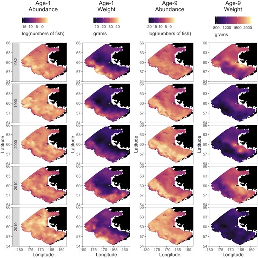
Model estimates of area-expanded abundance log(abundance, numbers of fish) and weight (grams) for age-1 and age-9 walleye pollock (G. chalcogrammus) for subset of years (1982, 1990, 2000, 2010, and 2019).

Open in new tab Download slide

The overall magnitude of spatial variation in size also differed among age classes. The youngest age classes showed the greatest variation across grid cells (Figure 3), with a CV of 42% for age-1 and 39% for age-2 pollock. There was a marked decline in variation for older ages. CV dropped to 30% for age-3 and further declined to ∼18–22% for each age classes 4–15+ .

Figure 3.

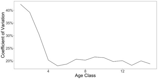
Spatial CV of estimated size-at-age of walleye pollock (G. chalcogrammus) in the Bering Sea for each age class, calculated as the standard deviation across all grid cells and all years divided by the mean across grid cells and years.

Open in new tab Download slide

There was also a trend of declining size-at-age over the study period for all but the youngest age classes at both the local and population level (i.e. the size-at-age matrix). Beginning in 2015 through 2019, there was a distinct, uniform decline in weight for age-8 pollock and older across the entire Bering Sea, while this was not evident in younger ages (e.g. see Supplementary Figure 4). At the population level, size-at-age from the first modelled year (1982) to the last modelled year (2019) declined by 24% for age-1 pollock, increased by 12–60% for age-2 through age-5 pollock, and declined by 15–30% for age classes 6–8, and 35–50% for age classes 9 and older (e.g. Figure 4 and Supplementary Figure 5).

Figure 4.

Size-at-age matrix (i.e. annual abundance-expanded population size-at-age) from model estimates (dashed line) and standard error (grey-shaded), compared to the simple empirical estimate (i.e. the simple empirical average, a non-spatially explicit weighted average of observations) (solid black line) for ages-1 (top panel) and 9 (bottom panel) walleye pollock. See Supplementary Figure 4 for all age classes.

Open in new tab Download slide

Our spatio-temporal size-at-age matrix differed from the simple empirical estimate (i.e. the non-spatially explicit, simple empirical average) of size-at-age. Though this non-spatial estimate somewhat tracked fluctuations in the model size-at-age, it often fell outside the confidence range (Figure 4 and Supplementary Figure 5).

Question 2: impact of spatial and spatio-temporal variation on size-at-age matrix

The size-at-age matrix was impacted by both spatial and spatio-temporal variability. Both latent persistent spatial and transient spatio-temporal patterns in size across the Bering Sea contributed to the fluctuations in the population-level size-at-age matrix. Population-level size-at-age that excluded spatial or spatio-temporal variation differed from the full model (Figure 5 and Supplementary Figure 6), though the magnitude of the impact varied between age classes. Spatial variation had the largest impacts in age-1 and ages 5–7, with 10–25% average impact on annual size-at-age. However, for the remaining age classes, the impact of spatial variation was relatively minor, with an average difference of 8–14% for age-8–14, and almost zero impact on age-3 and age-15. Spatio-temporal variation had an overall lower impact on more age classes, ranging from 2 to 8% for age-1 and age-4–15, and only had a larger impact on age-2 and age-3 pollock (14 and 20%, respectively). Overall, spatial and spatio-temporal variation had relatively similar magnitude of impact on the size-at-age matrix.

Figure 5.

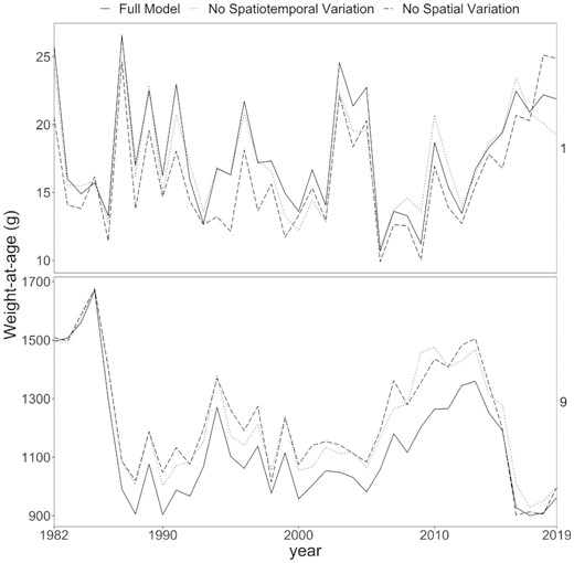
The size-at-age matrix (i.e. annual abundance-expanded population size-at-age) from the full model, including spatial, spatio-temporal, and temporal variation (solid black line) compared to (1) removing spatial variation (dashed line) and (2) removing spatio-temporal variation (dotted line). See Supplementary Figure 5 for all age classes.

Open in new tab Download slide

Question 3: contribution of local variation in size vs. abundance to size-at-age matrix

Annual fluctuations in the weight-at-age matrix were almost entirely due to changes in local size between years, rather than shifts in local fish abundance (Figure 6). Inter-annual fluctuations in size-at-age were markedly dampened when local variation in size-at-age was removed, but were not substantially changed when local variation in abundance was removed. Incorporating local variation in abundance-at-age but holding local size constant caused an 11–19% average difference (Figure 6 and Supplementary Figure 7). Including local changes in fish size while holding local abundance-at-age constant on average caused only a 2–8% average difference (Figure 6). Overall, accounting for the changes in local size-at-age processes year-to-year had a substantial impact when extrapolating to the population level, while compensating for local changes in fish density did not greatly change the size-at-age matrix value.

Figure 6.

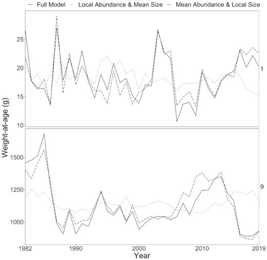
The population size-at-age matrix from the full model (i.e. calculating the abundance-expanded size-at-age with both local size-at-age and local abundance-at-age) (solid black line) compared to the size-at-age matrix calculated using (1) local abundance but mean size-at-age (i.e. showing the contribution of local size-at-age) (dotted line) and (2) mean abundance but local size-at-age (i.e. showing the contribution of local abundance) (dashed line). See Supplementary Figure 6 for all age classes.

Open in new tab Download slide

Question 4: stock assessment comparison

The spatio-temporal size-at-age matrix did marginally change estimated annual biomass and numbers of fish from the walleye pollock stock assessment (Figure 7) compared to the simple empirical mean. The stock assessment model using our spatio-temporal size-at-age resulted in a slightly improved fit than a model using the simple empirical estimate (ΔAIC = 3.6). In particular, the spatio-temporal model resulted in marginally better predicted biomass in the year 2003 (Figure 7), when the observed biomass in the bottom trawl survey was anomalously higher than the model estimates for that year. The spatio-temporal model was able better avoid the underestimation and capture the higher biomass that was a closer fit to the survey observation. A similar pattern is seen in 1991, though there is less divergence between the model and observation than 2003. The spatio-temporal size-at-age matrix generally estimated lower size-at-age than the simple empirical estimate in 1991, except for much higher estimates in the oldest age-classes of 13–15+ . In 2003, size-at-age was also higher in the spatially explicit model in the oldest age classes, but also in some younger ages (Supplementary Figure 5). There was essentially no difference in the estimated numbers of fish in the stock by the assessment model between size-at-age methods until the most recent several years (2015–2021), when the numbers of fish estimated using the spatio-temporal size-at-age are consistently higher than the simple empirical estimate (Figure 4). This suggests that local-scale variation in weight did manifest in the demographic patterns of the population, and that accounting for these structures scaled up to impact the estimation of population-level metrics.

Figure 7.

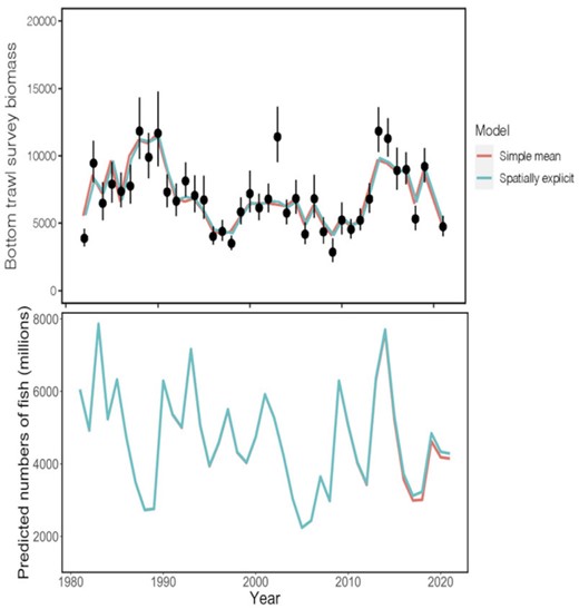
Walleye pollock biomass from bottom trawl survey (top) and predicted numbers of fish (bottom) estimated from stock assessment model (Ianelli et al., 2021) using spatio-temporal size-at-age matrix (blue) and from the simple empirical estimate (a non-spatially explicit weighted average of observations) (red), compared to observed biomasses (black points).

Open in new tab Download slide

Discussion

We developed and demonstrated a population-level size-at-age matrix that accounts for both inherent differences in size-at-age between habitats across the region and movement of fish (i.e. shifts in distribution) among patches with smaller or larger size. Local spatial variation in size-at-age, rather than local changes in abundance, largely governed variability in the resulting weight-at-age matrix. Accounting for spatial and spatio-temporal variation in local size-at-age therefore considerably impacts the estimated population size-at-age. Spatio-temporal models, such as with VAST as done here, of abundance (e.g. Fenske et al., 2020) and age composition (e.g. Thorson and Haltuch, 2018; O'Leary et al., 2020) have been used in stock assessments previously, but to our knowledge, this is the first example of the approach being applied to size-at-age. While the stock assessment in our study was relatively robust to the method used to calculate survey size-at-age, climate change will make it increasingly important for fisheries to account for the rapid pace of distribution shifts and environmental changes that species are likely to experience. The overall framework implemented here (spatio-temporal estimation and abundance-expansion of size-at-age) could be widely applied to other systems and stock assessments to evaluate the sensitivity of estimates to changing species distributions and local changes in productivity and growth.

This study highlights large decreases in size-at-age for pollock. Our model showed a general trend of a decline in size-at-age between the beginning and end of the study period in all but the youngest age classes of pollock. While age-2 through age-5 pollock did not see a decline, sizes of age-1 and ages-6–15+ in the final year of the study period (2019) were 15–50% lower than at the beginning (1982). This aligns with recent reports from fishers, who noted smaller than usual pollock in 2020 and 2021 catches (Ianelli et al., 2021).

This decline may be due to changes in environmental conditions or size-selective fishing. Declines in fish growth and size with ocean warming are expected due to increased metabolic demand and reduced oxygen availability in higher sea temperatures (Daufresene et al., 2009; Gardner et al., 2011) and have been widely documented (e.g. Baudron et al., 2014; van Rijn et al., 2017). For instance, Pacific halibut mean size-at-age has declined at a similar magnitude to our study (Holsman et al., 2018), and has been attributed to both sea temperature (Holsman et al., 2018) as well as interspecific competition, density-dependent effects, and size-selective fishing (Clark and Hare, 2002; Sullivan et al., 2018). Higher temperatures are also likely to reduce body size in larger and older individuals more than smaller and younger individuals (Ikpewe et al., 2020; Lindmark et al., 2022; Oke et al., 2022). Over the last several years (∼2016–2021), the Bering Sea has experienced warmer than average temperatures (Ianelli et al., 2021). The age-class patterns we observed and recent environmental conditions of the Bering Sea would be consistent with an age-specific growth response to environmental conditions.

Size-selective fishing may also have contributed to the decline in size-at-age. Fishery-induced declines in size-at-age have been documented in numerous fisheries (Sharpe and Hendry, 2009) such as Pacific halibut (Sullivan, 2016, Sullivan et al., 2018) and northern cod (Krohn and Kerr, 1997). Size-selective fishing can lead to smaller body size through evolutionary pressure (e.g. Swain et al., 2007; Jorgensen et al., 2009) causing heritable genetic change (Uusi-Heikkila et al., 2015), phenotypic plasticity (Fenberg and Roy, 2008), or the higher removal of faster-growing individuals of a population (i.e. the “Rosa Lee phenomenon”, Kraak et al., 2019). In the Bering Sea pollock fishery, vessel operators pursue pollock that are optimal for cost-efficient processing and market demand, and some vessels have modified gear to exclude smaller pollock (Ianelli et al., 2021). Further exploration of the links between spatio-temporal variation in size-at-age of walleye pollock in the Bering Sea and environmental conditions would help clarify the possible cause of declining size-at-age.

This spatio-temporal model of size-at-age can improve stock assessments in several ways. Our estimated weight-at-age matrix incorporated the extensive local variation in size across the eastern Bering Sea. By jointly estimating size and abundance at a fine spatio-temporal scale, we also compensated for uneven distributions in fish abundance and shifts in distribution of fish throughout the region when expanding the local size estimates to the population size-at-age matrix. While the stock assessment was not substantially impacted by the method for generating the size-at-age matrix, the spatio-temporal and abundance-expanded size-at-age matrix did slightly improve the fit of the model to the biomass survey data. For instance, the spatio-temporal size-at-age was able to slightly improve the model’s ability to capture the anomalously high biomasses observed in the bottom trawl survey in 2003 (and to a lesser extent in 1991). Lastly, a spatio-temporal model, as done in this study, can help extrapolate in time and space to account for shifting survey and stock extents (O'Leary et al., 2020, 2022; Adams et al., 2021). For instance, in this study, weight observations of pollock in the northern Bering Sea were not available, and there is sparse data from that region because of limited surveys. Additionally, our joint modelling approach allows the size-at-age matrix to include both uncertainty in estimates of size and uncertainty in estimates of abundance. Spatio-temporal approaches have become more common practice in some components of the stock assessment (such as biomass and age composition). While we did not see a marked change in the stock assessment outcome from our spatio-temporal method to size-at-age, accounting for spatio-temporal variation in other demographic metrics, such as size-at-age in this study, are the logical next step and will improve methodological consistency across a stock assessment.

Extending our spatio-temporal framework of size-at-age to fishery size data could be particularly beneficial because fishery-dependent data tend to have more pronounced spatial variation in fishing effort. There are differences in selectivity between fleets (e.g. gear characteristics such as depth of fishing) and unbalanced sampling in areas of higher, or lower, fish abundance due to fishers preferentially targeting areas based on convenience, safety, profitability, etc. (Maunder et al., 2020). A spatio-temporal model of size-at-age from fishery data consequently would require additionally accounting for catchability and selectivity when weighting size-at-age by catch (Maunder et al., 2020; Thorson et al., 2020). Stock assessments can be sensitive to how fishery size-at-age is estimated (Punt and Smith, 2001). An accurate fishery size-at-age is necessary for correctly determining the number of fish caught by the fishery when landings are measured in weight and, consequently, how actual fishing mortality compares to management limits (Ianelli et al., 2021). This study shows that it is feasible to take the grid-level output of size and abundance estimates from VAST and calculate a population average size-at-age, first weighting density by area and then weighting size by abundance. Including catchability covariates and weighting size by catch and fitting to fishery data would be a tractable extension of the model used in this study.

Our model showed extensive local-scale differences in size-at-age across the region and across years, suggesting that there is significant variation in local growth processes. Certain areas may have intrinsic conditions that make them more or less favourable for growth (e.g. Williams et al., 2003, Begg and Martensdottir, 2002), contributing to the persistent spatial differences seen. Spatial patterns in pollock size have been previously observed; for instance, pollock in the northwest area have typically been found to be smaller than those in the southeast (Ianelli et al., 2021). Additionally, we saw annual differences in the spatial patterns that may indicate more transient changes in habitat conditions. We also saw some evidence of local shifts in abundance, though this was not as predominant as local variation in size-at-age. Passive dispersal and habitat selection can impact size-at-age if fish move to optimize foraging resources, to access spawning grounds, or to avoid competition or predators (Hanselman et al., 2015). Fish may also make dynamic migratory decisions based on energetic status, resulting in larger individuals migrating to different habitats than smaller individuals, such as has been seen in sablefish (Hanselman et al., 2015). In this study, however, local changes in growth processes, rather than shifts in distribution, seemed to be the principal driver of size-at-age.

Our spatio-temporal model of size-at-age also informs our understanding of how these local spatial and temporal patterns in size affect population-scale productivity. This has been identified as a “Grand Habitat Challenge” (Thorson et al.,2021). Here, we developed a model of local size at a fine spatial scale, and expanded it to population-level abundance and productivity through the stock assessment. We show that persistent habitat conditions (spatial variation) and annual fluctuations in the suitability of a habitat for growth (spatio-temporal variation) caused local-scale variation in size-at-age over space and between years. Incorporating the variation in local size-at-age was the main driver of the annual population size-at-age (i.e. the size-at-age matrix). This suggests that variation in local growth processes across years did have an impact on population-level demographic metrics. In this study, we therefore show a feasible approach to incorporate fine-scale local demographic processes into population-level assessments.

Being able to predict how demographic rates, such as growth and size, may respond to environmental change will also be crucial for incorporating the effects of climate change into stock assessment models (Punt et al., 2021). In the Bering Sea, climate change is likely to alter environmental conditions known to impact walleye pollock demographics. Declining sea ice cover and associated declines in zooplankton may reduce food availability and impact growth processes (Hunt et al., 2008; Mueter and Litzow, 2008; Hunt et al., 2022) and recruitment (Mueter et al., 2011), and reduced bottom sea temperatures (i.e. the “cold pool extent) impacts a suite of demographic characteristics (Gruss et al., 2021). A model that can estimate size-at-age at fine spatial and temporal scales will enable better predictions of size-at-age, and the associated impacts on yield-per-recruit and other elements of the stock assessment, under future climate scenarios. For simplicity, in this study, we did not integrate environmental or catchability covariates or forecast future size-at-age. Rather, we focused on an initial assessment of the feasibility of applying spatio-temporal models to size-at-age and abundance for stock assessments. It can often be difficult to identify the specific environmental features that cause observed variation in fish populations (Thorson et al., 2017; Dambrine et al., 2021), and addressing the latent spatio-temporal as done here was a tangible first step. The framework presented here can be expanded to incorporate environmental covariates and used for short-term forecasting.

Supplementary data

Supplementary material is available at the ICESJMS online version of the manuscript.

ACKNOWLEDGEMENTS

We would like to specifically thank Cecilia O'Leary and Caitlin Allen-Akelsrud for their help and guidance on pulling together the various data sources. Special thanks to the bottom trawl survey team and Age and Growth Program at the NOAA Alaska Fisheries Science Center for the data that make this work possible. We also thank Paul Spencer and Christine Stawitz and the two anonymous reviewers for helpful comments on a previous draft.

Funding

This publication was partially funded by the Cooperative Institute for Climate, Ocean, & Ecosystem Studies (CIOCES) under NOAA Cooperative Agreement NA20OAR4320271, Contribution No. 2022-1205 and by the National Pacific Research Board Grant #1805. J.I. was supported partly by a CICOES Graduate Student Award (Contribution No. 2022-1205) and by the National Pacific Research Board Grant #1805.

Data availability

The data underlying this article will be shared on reasonable request to the corresponding author.

Conflict of interest

The authors have no conflicts of interest to declare.

References

Adams

Brooks

Legault

Barrett

Chevrier

2021

Quota allocation for stocks that span multiple management zones: analysis with a vector autoregressive spatiotemporal model

Fisheries Management and Ecology

417

–

427

Month:	Total Views:
January 2023	313
February 2023	64
March 2023	197
April 2023	93
May 2023	63
June 2023	48
July 2023	29
August 2023	47
September 2023	70
October 2023	45
November 2023	71
December 2023	59
January 2024	67
February 2024	37
March 2024	37
April 2024	46
May 2024	65
June 2024	39
July 2024	55
August 2024	32
September 2024	47
October 2024	48
November 2024	37
December 2024	24
January 2025	51
February 2025	47
March 2025	38
April 2025	35
May 2025	26

Article Contents

Incorporating distribution shifts and spatio-temporal variation when estimating weight-at-age for stock assessments: a case study involving the Bering Sea pollock (Gadus chalcogrammus) Open Access

Abstract

Introduction

Methods

Data compilation

Model structure

Annual population size-at-age

Question 1: spatial and temporal patterns of size-at-age

Question 2: impact of spatial and spatio-temporal variation on size-at-age matrix

Question 3: contribution of local variation in size vs. abundance to size-at-age matrix

Question 4: stock assessment comparison

Results

Question 1: spatial and temporal patterns of size-at-age

Question 2: impact of spatial and spatio-temporal variation on size-at-age matrix

Question 3: contribution of local variation in size vs. abundance to size-at-age matrix

Question 4: stock assessment comparison

Discussion

Supplementary data

ACKNOWLEDGEMENTS

Funding

Data availability

Conflict of interest

References

Supplementary data

Citations

Views

Altmetric

Email alerts

Citing articles via

Latest

Most Read

Most Cited

This Feature Is Available To Subscribers Only

Incorporating distribution shifts and spatio-temporal variation when estimating weight-at-age for stock assessments: a case study involving the Bering Sea pollock (Gadus chalcogrammus)