


SUMMARY
Full-waveform inversion (FWI) has been proven to be an effective tool for high-resolution multiparameter imaging of the shallow subsurface. It has been shown that the Gauss–Newton (GN) optimization method uses the off-diagonal information contained in the Hessian matrix and can increase resolution and mitigate crosstalk in multiparameter viscoelastic FWI. In this work, we demonstrate the advantages of GN viscoelastic FWI over the conventional FWI with a conjugate gradient optimization method by using synthetic examples. We also investigate the potential of shallow seismic-wave 2-D viscoelastic FWI as a method for high-resolution hydrogeological characterization. The GN viscoelastic FWI is applied to two orthogonal profiles acquired at the Krauthausen natural laboratory (Germany). The groundwater table is located at around 2 m, which nicely agrees with an abrupt increase of P-wave velocity in the inverted results. FWI also reveals a low S-wave velocity layer at the depth of 4–6 m with high Poisson’s ratio values close to 0.5, which corresponds to a saturated sand layer known from previous studies. A K-mean cluster analysis is used to further analyse the multiparameter FWI results. By considering the derived Poisson’s ratio, P- and S-wave velocities, we convert the complex relationship between the multivariate data into a lithological meaningful zonation of the shallow subsurface. By comparing the lithological units in the alluvial aquifer with the cone penetration tests clusters, we conclude that the divided facies describe valuable characterization information about the heterogeneity and connectivity of the aquifer. This experiment indicates that the multiparameter models derived by viscoelastic FWI contain useful information for high-resolution aquifer characterization, and the potential of multiparameter FWI combined with cluster analysis in shallow subsurface characterization is encouraging.
1 INTRODUCTION
A reliable investigation of the near-surface models is of fundamental importance in geophysical and geotechnical surveys. Near-surface wavefields are dominated by Rayleigh waves, which have a higher signal-to-noise ratio compared to body waves (Socco et al. 2010). Multichannel analysis of surface waves method (MASW) is proposed to obtain shear wave velocity (VS, Xia et al. 1999). In the application of the MASW, dispersion curves are picked according to the maximum energy tracing on the dispersion image obtained from the multichannel recording system. By inverting the picked phase velocities, S-wave velocity in shallow layers can be estimated. However, the dispersion-based methods face limitations due to the strong lateral heterogeneities. Secondly, shallow-seismic models which contain large velocity contrasts could generate seismograms with dominant higher modes of surface waves (Boaga et al. 2013; Gao et al. 2014, 2016; Mi et al. 2020). In this case, the reliability of the inversion result depends on the correct identification and estimation of multimodal dispersion curves.
Full-waveform inversion (FWI) is a waveform fitting method by iteratively minimizing the differences between the observed and modelled seismograms. It has the potential to provide high-resolution multiparameter models for complex geological structures. With the computational power increases, it has become a novel technique to perform surface wave FWI to reconstruct 2-D near-surface models (Romdhane et al. 2011; Tran et al. 2013; Groos et al. 2014; Zhang et al. 2015; Pan et al. 2016; Groos et al. 2017; Dokter et al. 2017; Li et al. 2017; Pan et al. 2019; Pan & Gao 2020), and also been investigated in 3-D cases (Mirzanejad & Tran 2019; Pan et al. 2021; Irnaka et al. 2022). However, most of the previous studies invert for S-wave velocity only and neglect attenuation effects or simply implement a passive-viscoelastic FWI with a fixed attenuation model during the forward modelling to compensate for viscoelastic effects. When a high level of heterogeneity of attenuation exists in the shallow subsurface, neglecting the viscoelastic effect during the inversion might deteriorate the S-wave velocity results (Groos et al. 2014; Gao et al. 2020).
For a better explanation of the subsurface with more realistic parameters, multiparameter FWI is proposed to extract detailed geological information (Virieux & Operto 2009). Simultaneous reconstruction of multiple physical parameters would suffer from the crosstalk effect caused by the ambiguities between the different parameter classes (Köhn et al. 2012; Métivier et al. 2013; Operto et al. 2013; Fabien-Ouellet et al. 2017). Conventional FWI algorithms are generally implemented via gradient-based methods, such as the steepest descent (SD) method, and the nonlinear conjugate gradient (CG) method, cannot decipher the model perturbation numerically in the gradient (Gao et al. 2020). The choice of the different parametrizations would influence the final inversion results. Analysis of the sensitivity of different parametrizations have been investigated (Köhn et al. 2012; Operto et al. 2013; He & Plessix 2017; Pan et al. 2020; Gao et al. 2021). Accounting for the Hessian matrix during the inversion helps to mitigate the crosstalk effects (Pratt et al. 1998; Métivier et al. 2013; Pan et al. 2018; Yang et al. 2018). However, expensive computational and storage costs make the calculation of the Hessian matrix and its inverse unaffordable for large-scale inverse problems. The truncated Newton (TN) method requires matrix-free formalism by obtaining the Hessian-vector products with the second-order adjoint-state method, aims at reducing the computational burden of Hessian-based FWI (Métivier et al. 2013; Yang et al. 2018; Gao et al. 2021).
Compared to TN method, the Gauss–Newton (GN) method could also be a candidate strategy, which is a simplification of TN method where the cross term in the Hessian matrix is omitted. One advantage of the GN method over Newton’s method is that the Hessian matrix will be obtained as a positive definite matrix, benefit for a better convergence (Virieux & Operto 2009). GN method is adopted in acoustic FWI (Métivier et al. 2013), and visco-acoustic FWI (Yang et al. 2018). Later, Chen & Sacchi (2020) also adopt an elastic matrix-free FWI algorithm with GN optimization in the time domain, which inverts for P- and S-wave velocities (VP and VS) simultaneously and presents numerical examples in a 2-D elastic case.
Multiparameter FWI could provide different seismic properties (velocity, attenuation and density) of the Earth. Instead of assessing individual parameter classes, a combined interpretation of multivariate parameter classes could further be used to delineate the lithological facies of the subsurfaces. Cluster techniques can identify different lithological units with dominant properties (Tronicke et al. 2004; Dietrich & Tronicke 2009; Gueting et al. 2015). In this way, different lithological facies like sand and gravel layers differ in the seismic parameters could be distinguished. In this paper, we present a combined work of multiparameter FWI method and cluster analysis to investigate the potential of shallow seismic-wave 2-D viscoelastic FWI as a method in high-resolution hydrogeological near-surface characterization.
Motivated by the approach of the matrix-free GN algorithm, we employ a viscoelastic shallow-seismic FWI in time domain for simultaneous reconstruction of five parameters: VP and VS, the quality factors of P and S waves (Qp and Qs), and the density (ρ), in two numerical tests and a field data experiment. The paper is organized as follows. In Section 2, we briefly introduce the methodology of FWI, together with a general implementation of GN FWI. In Section 3, we present the numerical results to assess the benefit of the GN method over the CG method. In Section 4, we show a field experiment, which is conducted at the Krauthausen test site located in Northwest Germany. Seismic data were acquired along two orthogonal lines. The seismic FWI is applied to estimate both VP and VS, attenuation of P and S waves, and thereby Poisson’s ratio. The outcomes of the inversion enable us to understand in detail the lateral variation in layer thickness and properties under the profiles. Later, a cross-sectional image presents the spatial distribution of the layers indicating the connectivity of the obtained two profiles. A K-mean cluster analysis (Macqueen 1967) is conducted for the facies classification by considering their VP, VS and Poisson’s ratio. The validity of the classified results is verified by comparing them with the results from cone penetration tests (CPTs).
2 METHODOLOGY
FWI, as a data-fitting iterative procedure, aims to minimize the differences between the simulated data and the measured data defined as,
Here, the model properties (e.g. velocities, attenuation and density) are marked by |$\boldsymbol {m}$|. Further, |$\boldsymbol {d}_{\mathrm{ obs}}$| and |$\Phi (\boldsymbol {m})$| represent the measured and synthetic seismograms computed with the model |$\boldsymbol {m}$|, associated with the receiver |$\boldsymbol {x}_r$| and the source |$\boldsymbol {x}_s$|, respectively. Nr and Ns represent the total number of receivers and sources, respectively. And t is the time.
FWI is formulated as an optimization problem of the misfit function J. Given the large sizes of the unknown subsurface models, the inversion based on global optimization method is computationally expensive for solving problems (Xing & Mazzotti 2019). Hence, FWI is usually performed based on the iterative local optimization technique in which the gradients can be calculated efficiently by the adjoint-state method (Plessix 2006). For local nonlinear optimization FWI, an iterative sequence |$\boldsymbol {m}_{n+1}$| is obtained by starting from an appropriate initial guess |$\boldsymbol {m}_0$|, and then iteratively updated with a descent direction |$\Delta \boldsymbol {m}_n$|:
where n is the iteration number. And the step length λ at iteration n can be estimated through a line search process with parabolic fitting (Nocedal & Wright 2006). The model perturbation, |$\Delta \boldsymbol {m}_n$|, can be given by gradient-based (e.g. SD and CG) and Newton-based method (e.g. TN and GN methods). Multiparameter FWI is challenging due to the potentially strong crosstalks between the different parameter classes (Virieux & Operto 2009; Operto et al. 2013). Updating the model perturbation with gradient only cannot decipher different parameters. Researches show that Newton-based methods generate less crosstalk and artefacts in the reconstructed models (Métivier et al. 2013; Yang et al. 2018; Gao et al.2021).
Within the Newton optimization framework, |$\Delta \boldsymbol {m}_n$| could be calculated as a solution of the linear equation:
where G is the gradient vector (the first derivative of J), given as:
and H is the Hessian matrix (the second derivative of J), given as:
In the aforementioned equations, the † represents the adjoint operator. And the |$\frac{\partial \Phi }{\partial \boldsymbol {m_i}}$| is the partial Fréchet derivative of the forward operator Φ with respect to the model parameters |$\boldsymbol {m_i}$|, also noted as Φ′ for simplicity. When ignored the second part in eq. (5), it becomes GN Hessian matrix HGN, leading the eq. (3) becomes a simplification of Newton’s equation as:
Further be rewritten as:
In the general definition of GN method, the GN Hessian HGN needs to be calculated, which faces prohibitively expensive storing and computation. In this paper, we use the GN FWI with matrix-free formalism to solve eq. (7). The general scheme includes two loops: an external loop for GN update and the inner loop to solve eq. (7) by the linear conjugate gradient method. For the self-contentedness of this paper, the general implementation of the time-domain viscoelastic PGN method algorithm is presented in Algorithm 1. During the inversion, a unity-based normalization is used to promote the sensitivity of weak parameters as Yang et al. (2018). From the view of exploration imaging, the Fréchet derivative operator Φ′ functions as the Born modelling operator (step 9 in Algorithm 1) while the adjoint Fréchet derivative operator Φ′† to data residuals is equivalent to an RTM algorithm applied to data residuals instead of data (step 7 in Algorithm 1). The expressions for operators of the associated equations in Algorithm 1 are shown in Appendix B for the brevity of the paper. More detailed description derivation about the multiparameter FWI procedure with GN optimization, the reader could refer to Bohlen et al. (2021, also called with CG-REGINN).
Time domain Gauss-Newton method FWI in matrixfree formalism
 |
|
Time domain Gauss-Newton method FWI in matrixfree formalism
|
|
3 NUMERICAL COMPARISON
3.1 Model 1
One of the challenges in multiparameter FWI is the parameter crosstalk problem caused by the overlaps of the Fréchet derivative wavefield. Overlaps between the Fréchet derivative wavefield are inevitable (Pan et al. 2018). In the near-surface case we mainly deal with transmitted wavefields that are best characterized in terms of phase velocities instead of impedances which describe reflections which we do not observe. This leads us to the definitions of VP and VS as primary inversion parameters. The other parameters S-wave attenuation (τs), P-wave attenuation (τp) and density (ρ) then follow naturally. This optimal set of inversion parameters thus becomes VS, VP, τs, τp and ρ. The optimal performance of this parametrization has been verified by many synthetic reconstruction tests, for example Groos et al. (2014).
Notations for the parameters used in the FWI algorithm.
| VS | S-wave velocity vector |
| VP | P-wave velocity vector |
| ρ | Density vector |
| |$\boldsymbol {v}$| | Velocity vector of the forward equation |
| |$\boldsymbol {\sigma }$| | Stress vector |
| |$\boldsymbol {\eta _l}$| | Memory variable corresponding to the stress tensor |$\boldsymbol {\sigma }$| |
| |$\boldsymbol {\tau _{\sigma ,l}}$| | Stress relaxation time of the lth Maxwell body |
| L | Total number of Maxwell bodies |
| τs | Attenuation levels of S waves |
| τp | Attenuation levels of P waves |
| |$\boldsymbol {f}$| | External force |
| |$\boldsymbol {\mu _0}$| | Relaxed S-wave moduli |$\mu _0=\frac{\rho V_S^2}{1+\alpha \tau _S}$| |
| |$\boldsymbol {\pi _0}$| | Relaxed P-wave moduli |$\pi _0=\frac{\rho V_P^2}{1+\alpha \tau _P}$| |
| ω0 | Reference frequency, peak frequency of the source wavelet or observed data |
| α | To ensure the waves propagate with the model phase velocity ( |$\alpha =\sum _{l=1}^{L}\frac{\omega _0^2\tau _{\sigma ,l}^2}{1+\omega _0^2\tau _{\sigma , l}^2}$|) |
| C | Linear map defined as |$C\left(\mu _0,\pi _0\right)\boldsymbol \varepsilon \left(\boldsymbol {v}\right)=2\mu _0\boldsymbol \varepsilon (\boldsymbol {v})+\left(\pi _0-2\mu _0\right)\mathrm{tr}\left(\boldsymbol \varepsilon (\boldsymbol {v})\right)\boldsymbol {I}$|, where |$\boldsymbol \varepsilon \left(\boldsymbol {v}\right)=\frac{1}{2}\left[\left(\nabla _x{\boldsymbol {v}}\right)^T+\nabla _x\boldsymbol {v}\right]$| |
| |$\boldsymbol {\sigma _0}$| | |$\boldsymbol {\sigma }+\sum _{l=1}^{L}\tau _{\sigma ,l}\boldsymbol {\eta _l}$|, new transformation to symmetrize the operators Zeltmann (2019) and Kirsch & Rieder (2019) |
| |$\boldsymbol {\sigma _l}$| | |$-\tau _{\sigma ,1}\boldsymbol {\eta _l}$| |
| |$\boldsymbol {w}$| | Velocity vector of the backward eq. (B3) |
| |$\boldsymbol {\psi _l}$| | Stress vector of the backward eq. (B3) |
| |$\boldsymbol {\bar{v}}$| | Velocity vector of the second forward wave eq. (B4) |
| |$\boldsymbol {\bar{\sigma }_l}$| | Stress vector of the second forward wave eq. (B4) |
In this section, we adopt synthetic model (model 1) which is used in Gao et al. (2021) to demonstrate the validity of the viscoelastic GN FWI approach. The true model consists of a depth-dependent 1-D background model. Two 5-m wide rectangular anomalies are designed on five parameters at two different depths (1 and 4 m, Fig. 1). Eight shots are placed in the horizontal direction from X= 20 to 90 m with a shot interval of 10 m. A 40 ms delayed Ricker wavelet with a central frequency of 30 Hz is generated as a vertical-force source. 71 receivers are distributed along the surface starting from 20 to 90 m. In Fig. 2, the snapshots of wavefields at different times are displayed with letters to show the wave types. The Rayleigh waves (R) are dominated in the wavefields that propagate along the free surface. Besides the P and S waves, it also contains diffraction wavefields caused by the anomalies.
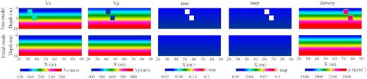
First numerical example (model 1) for multiparameter reconstruction. The first and second rows represent the true and initial models, respectively.
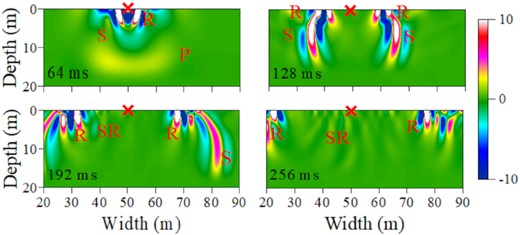
The wavefield snapshots at t = 64, 128, 192 and 256 ms of the vertical particle motions. The cross denotes the source on the free surface. The letter of ‘S’, ‘P’, ‘R’ and ‘SR’ represent the S, P, Rayleigh and scattered Rayleigh waves.
In our examples, the mainly targeted signals used in near-surface FWI are surface waves, which propagate along the free surfaces with higher energy (Fig. 2). We transform the raw shot gather (Fig. 3a) of shot 1 into frequency-phase velocity domain (Fig. 3b), in which the longest (20.88m) and shortest (1.29 m) wavelength of the fundamental mode of Rayleigh wave are marked with white crosses. The longer wavelengths penetrate deeper and are more sensitive to the properties of the deeper layers. While short wavelengths are sensitive to the physical properties of surficial layers. The currently accepted rule of the maximum penetration depth is half of the longest wavelength in homogeneous medium (Rix & Leipski 1991). In this example, the anomaly is 5 m wide with 2 m thickness. Thus, we can retrieve the anomalies of the surficial layers.
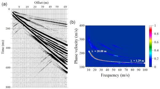
(a) The seismogram of shot 1. (b) The corresponding dispersion image of shot 1 obtained by high-resolution linear Radon transform (Luo et al. 2008). The white plus signs are used to mark the longest and shortest wavelengths of the fundament mode. The wavelength is calculated by the ratio of the phase velocity and the corresponding frequency.
The initial models are the background model with increasing values (Fig. 1). For comparison, we also present the inverted models using the CG approach. For both optimization methods, a pre-conditioner which is calculated by an approximated inverse of the Hessian matrix by using its diagonal term (Gao et al. 2021) is added to the optimization. Additionally, we set the source time function (STF) as known for simplicity, and adopt a multistage inversion strategy (Bunks et al. 1995) with progressive frequency bands of 0–25, 0–35, 0–45, 0–60 and 0-80 Hz during the inversion to avoid the cycle skipping. All five parameters are updating without restarting and reinitializing. In each frequency stage, a minimum of 10 iterations are performed. And the inversion proceeds to the next frequency stage when the relative decrease of the L2 misfit is less than 1 per cent.
The gradients of the first iteration and the final inversion results of two different optimization methods are shown in Fig. 4. In contrast, the shallow high VS anomalies obtained by the two optimization methods are similar thanks to the high sensitivity of Rayleigh waves to VS. However, the deeper low VS anomaly from the PGN is better reconstructed compared to the PCG results. In this numerical example, the VS models suffer crosstalk effects projected from the density anomalies in the PCG, and could be mitigated when considering the PGN optimization. In the PCG method, the gradient does not provide the correct order of the model perturbation, while the PGN method can bring the true orders of the magnitude. Thus, the gradients showed here are normalized for comparison. As Fig. 4 shows, the PGN method could mitigate the crosstalks (blue rectangle). The fewer residuals in the Rayleigh waveform (Fig. 5d) confirm that S-wave velocity results are better reconstructed. The inverted low VP anomalies from the PGN method show nice reconstruction compared with the VP results from the PCG method, which cannot be retrieved. The P-wave arrivals’ residuals in the PGN results are smaller than the PCG results, indicating a better reconstruction of P-wave anomalies by the PGN method (Fig. 5d). In the inverted τs model from the PCG method, we can note that strong crosstalk effects from VS are projected into the results, together with weak crosstalk effects from secondary parameters such as density and VP anomalies. While the reconstructed τs model shows less crosstalk projected from VS anomalies in the PGN method. Concerning the weak parameter τp, the anomalies cannot be reconstructed by the PGN method, however, the crosstalks projected from the VP anomalies are mitigated compared to the results from the PCG. This is caused by the low sensitivity of the Rayleigh wave with respect to it. As to the ρ models, the crosstalks projected from the VS anomaly are mitigated and the deeper density anomaly is better delineated than the result from the PCG. It also can be noted in the gradients of first iteration that the crosstalk effect caused by the VS anomalies are mitigated by PGN method compared with PCG method. Additionally, the comparison of data misfits and the waveform residuals (Fig. 5) also verifies that the PGN outperforms the PCG. Worthy to note, two misfit curves almost coincide with each other at the first frequency stage. The main reason is that in the first few iterations the inversion is influenced by the updating of S-wave velocity due to the dominance sensitivity of the Rayleigh wave with respect to it. Besides, it is also because that we already include a pre-conditioner to approximate the diagonal of Hessian in both PCG and PGN.
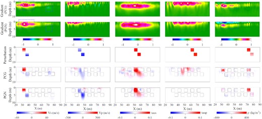
Numerical example comparisons for multiparameter reconstruction. The upper two rows represent the gradients of the first iteration of the PCG and PGN methods, respectively. The gradient are normalized for comparison. The lower three rows represent the true perturbation models, and reconstructed models from the PCG and PGN methods, respectively. τs and τp represent the attenuation levels of S and P waves (Bohlen 2002), respectively.
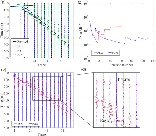
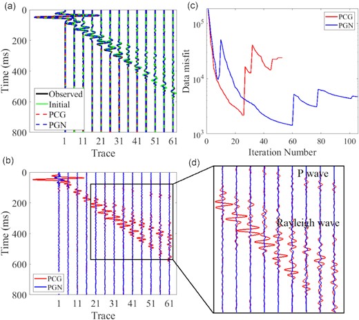
Data comparisons of model 1. (a) Seismograms for the final reconstructed model (dashed lines), initial model (green lines) and the true model (solid black lines) and (b) seismogram residuals for the PCG (red) and PGN (blue) methods. The red and blue lines represent the residuals from the PCG and PGN methods, respectively. Note that the residuals are magnified 10 times; (c) the L2 data misfit comparison between the PCG and PGN results and (d) zoom into far offset trace shown in (b).
3.2 Model 2
In the second synthetic example, we choose a realistic near-surface geological case in which the different model parameters are spatially correlated (Fig. 6). Here, we also investigate the performance of simultaneously inverting five parameters with PCG and PGN optimizations. The same inversion strategy as for the first example is applied for both PCG and PGN.
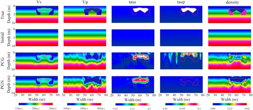
Near-surface synthetic multiparameter reconstruction test (model 2). The upper two rows represent the true and initial models, respectively. The lower two rows represent the reconstructed models obtained from the PCG and PGN methods, respectively.
Similar to the previous case, the subsurface structure is more clearly delineated by the PGN method. The inverted VS result shows clear interface boundaries as indicated in Fig. 6. The VP result is worse compared to VS due to its very low sensitivity to the Rayleigh wave. Nevertheless, the VP reconstruction can slightly be improved by PGN. The τs is also well reconstructed by PGN’s result. This indicate that the PGN method suffers less crosstalk projected from the other parameters. The very weak P-wave attenuation parameter τp cannot be reconstructed even by the PGN method. However, the crosstalks projected from the other parameters into τp are also mitigated by PGN. Furthermore, the density (ρ) structure is hard to be delineated by the PCG method, whereas the PGN method delivers much more accurate results, that is, a low-density anomalies in the upper layer and two high-density anomalies in the lower layer. The final data misfits and residuals between the observed seismogram and two different methods indicate that the PGN method outperforms the PCG method because of its power of the mitigation of crosstalk and thus can improve the accuracy and resolution of the final inverted results (Fig. 7).
Data comparisons of model 2. (a) Seismograms for the final reconstructed model (dashed lines), initial model (green lines) and the true model (solid black lines); and (b) seismogram residuals for the PCG (red) and PGN (blue) methods. Note that the residuals are magnified 10 times; (c) the L2 data misfit comparison between the PCG and PGN results and (d) zoom into far offset trace shown in (b).
Overall, two synthetic examples show that VS can be nicely delineated by both methods due to its dominance sensitivity on the Rayleigh waves. However, the GN optimization method can have a high chance to improve the accuracy of the multiparameter reconstruction results and mitigate the crosstalks caused by the other parameters. Besides, the final inverted results and data residuals in both examples prove that one relaxation mechanism is accurate enough to retrieve the subsurface models.
4 FIELD DATA APPLICATION
4.1 Description of the test site
The goal of the seismic survey was to characterize the hydrological situation at the Krauthausen test site. It is located in Northwest Germany between the cities Jülich and Düren and is built up by research center Jülich in 1993. In this well-studied Krauthausen test site, intensively investigations for the purposes of hydrological studies, including tracer experiments (Vereecken et al. 2000), multiple pumping tests (Li et al. 2007), CPTs (Tillmann et al. 2008) and geophysical imaging methods (Klotzsche et al. 2013, 2014; Gueting et al. 2015, 2017; Zhou et al. 2021; Haruzi et al. 2022) were conducted, by which can provide abundant useful information there. The present studies showed that the thickness of the uppermost aquifer was about 10 m and composed of alluvial terrace sediments (Fig. 8). The top of the aquifer was divided into three layers according to Döring (1997): the first layer (1–4 m depth) was a poorly sorted gravel layer; the second layer (4–6 m depth) was a well-sorted sand layer and a bottom layer composed of sandy to gravel grain size, which extended from 6 to 11.5 m depth. The ground water table would vary from 1 to 3 m in depth with annual season changes. Worthy to note, Fig. 8 represents a general profile with a conceptual model of the geological sequence for the aquifer area, which is just a simplification of the underground aquifer structure there.
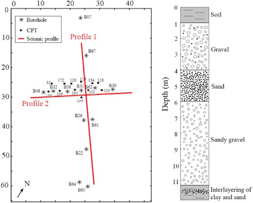
Left: schematic diagram of the studied Krauthausen test site including two seismic profiles (red solid lines) and adjacent boreholes and CPT positions. The asterisk and the dark dots represent the location of marked boreholes and the CPTs there, respectively. Right: a conceptual geologic image of the studied aquifer area referring to Döring (1997) and Tillmann et al. (2008).
Most recently GPR FWI revealed the heterogeneous variations of the uppermost aquifer with high resolution and also produce a detailed tomographic image with significantly improved result (Klotzsche et al. 2013; Gueting et al. 2015, 2017; Zhou et al. 2021; Haruzi et al. 2022). Besides, CPTs were performed in the centre of the test site by setting a 10 cm vertical sampling interval. In order to across the entire thickness of the studied aquifer area, each CPT vertical profile is drilling down to an average thickness of about 13 m (Gueting et al. 2015).
4.2 Data acquisition
In order to delineate the subsurface lateral variation in the Krauthausen test site, the seismic surveys were conducted along two perpendicular lines. The acquisition was implemented on the 2018 September 29 and 30 under relatively dry soil conditions (Athanasopoulos 2021). Two survey lines (P1 and P2) were set in the central part of the test site, where boreholes and CPTs were spaced closely there. The acquisition geometry of P1 consisted of 14 shots as vertical-force sources with an interval of 4 m and 48 receivers with an interval of 1 m. The acquisition geometry of P2 consisted of 11 shots generated by vertical-force sources with an shot interval of 4 m and 36 receivers with an trace interval of 1 m. The sources were generated by hammer blows hitting a steel plate. P1 crossed the boreholes 67, 31/62, 26/61, 22, 64 and 65, with the last one being the end of the receiver line. P2 was placed near Boreholes 48, 32, 38, 31, 62 and 30. A detailed map of the Krauthausen test site with two profiles is shown in Fig. 8 (Athanasopoulos 2021).
4.3 Inversion setup
An important requirement for the success of FWI is an adequate initial model (Virieux & Operto 2009). The MASW method can be considered as a traveltime inversion of Rayleigh waves and has been proved to be an effective way to generate very robust VS starting models for near-surface FWI (Groos et al. 2017; Pan et al. 2019; Irnaka et al. 2022). The comparison between the observed and initial seismograms is shown in Fig. 13. As we can see, the phase matching between them is much smaller than half a period, which means the initial model obtained by the MASW method is acceptable and accurate enough to avoid the cycle skipping. The initial 1-D VP model is obtained from the first-arrival times of the refracted waves. The initial ρ models are obtained through Gardner’s relationship. For the initial QP model, we assumed QP = 2*QS (Xia et al. 2012). Linear gradient models are used as the initial models for inversion. All five initial models are shown in the first column of Fig. 9. Before the inversion, a 3-D to 2-D transformation (Forbriger et al. 2014) must be applied to the field data. Each field seismogram is convolved with |$\sqrt{t^{-1}}$|, then multiplied with |$r_{\mathrm{ offset}}\sqrt{2*t^{-1}}$|, where t and roffset denotes the traveltime and source-to-receiver offset, respectively. Forbriger et al. (2014) demonstrated the suitability of the proposed method for viscoelastic case by numerical examples as well as the analytical considerations. And successful applications are performed (Schäfer et al. 2014; Groos et al. 2017; Pan et al. 2019). Aiming to decrease the non-linearity of the FWI and avoid the inversion being trapped into a local minimum, a sequential FWI workflow of low-pass filtered data with different bandwidths is applied (Bunks et al. 1995). In our example, the multistage inversion strategy with the frequency band starts with low-pass filter data with 0–15 Hz. The frequency range is progressively increased with 5 Hz until 40 Hz is reached, and the highest frequency band of 60 Hz is used in the last stage. The inversion will move to the next frequency stage if the relative decrease in the misfit value is less than 1 per cent. The central frequency of the initial STF is 30 Hz. Then, we estimate STFs by a stabilized deconvolution and set to update the STFs at the beginning of each frequency stage (Groos et al. 2014).
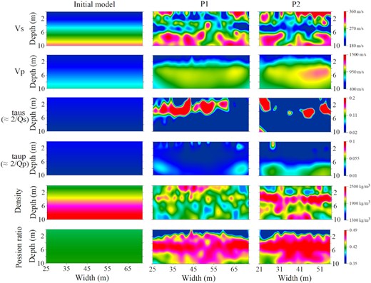
Final models below both profiles obtained by 2-D viscoelastic FWI with the PGN method. The initial models are represented in the first column. The second and third columna represent the reconstruction results of profiles 1 and 2, respectively.
4.4 Multiparameter FWI results
In this section, we present the inverted models obtained by the multiparameter viscoelastic FWI (Fig. 9). The reconstructed VS structure shows a high level of heterogeneity. Below the P1 profile, VS is low within the upper 2 m where the loamy soil layer has developed (Döring 1997; Gueting et al. 2015). Referring to the prior geological model (Fig. 8) of the test site (Tillmann et al. 2008), there is a poorly sorted gravel layer that exists in the depth of about 2–4 m, where the VS increases. A layer of low VS shows up at the depths of 4–6 m, which correlates well with previous studies that a sandy layer exists. Especially, the P2 profile shows a more continuous and distinct boundary of this sand layer, which can also be confirmed in Athanasopoulos (2021). Below this layer, VS increases, which agrees to the borehole information that the soil content change from sand to gravel. Overall, the S-velocity model is distinguished with horizontal layered structures. This result is consistent with stratigraphic layering (Fig. 8) in the gravel and sand deposits at the Krauthausen test site.
For VP results from both P1 and P2 profiles, both of them did not show strong horizontal heterogeneity compared to VS results. This low resolution can be attributed to the large wavelength of the Pwave at low frequencies. Nevertheless, consistent structures in the VP results can be observed. The inversion result shows VP = 380 m s−1 around in the shallow part and ρ = 2000 kg m−3 in the top 2 m, which corresponds to the property of unsaturated soil (Yilmaz 2015). According to the previous geologic surveys there (Fig. 8), the upper layers consisted of loamy soil. The P- and S-wave velocities for near-surface soil material with composition of sand, silt and clay always are much lower than those for subsurface rocks. The VP within a shallow soil column sometimes will be as low as 400 m s−1 or even lower, and may increase with depth of the soil column to 2000 m s−1 or higher. As to VS within a shallow soil column may be as low as 100 m s−1 or even lower, and may increase with the increasing of depth to 700 m s−1, which usually be characterized as the bedrock (Yilmaz 2015, p. 38). We can see the P-wave velocity is suddenly increased at the depth of about 2 m, where the groundwater table exists. It is confirmed that the effect of water saturation on VP is significant (Pasquet et al. 2016; Nagashima & Kawase 2021). This sudden increase could thus be an indicator of groundwater table level in the Krauthausen test site.
The inverted attenuation models of both profiles are given in Fig. 9. We inverted for the so-called τ parameter which relates to the quality factors of P and S waves by Qs ≈ 2/τs and Qp ≈ 2/τp (Bohlen 2002). For the τs results, we can observe clear strong attenuation anomalies located at the depth of 4–6 m. For the τp results, as can be seen, that the results are significantly contaminated by some artefacts. This could be interpreted as attenuation is the weakest parameter and can be easily affected by velocity and density errors (Fabien-Ouellet et al. 2017; Gao et al. 2020, 2021). As to the inverted density model (Fig. 9) in P1, the reconstructed results did not provide reliable information about the surface layers. With regards to the density model in P2, it delineates a high-density layer at about 3–5 m. As is known, Rayleigh waves have low sensitivity with regard to density, the reliability of the density results needed to be verified by some secondary data.
4.5 Poisson’s ratio
Experimental developments (Bachrach et al. 2000; Foti et al. 2002; Uyanik 2011) showed that the saturation could affect the P- and S-wave velocities. This gives a hint that the joint studies of VP and VS, especially by estimating Poisson’s ratio could provide a suitable evaluation of the saturation of aquifer characterization (Bachrach et al. 2000; Konstantaki et al. 2013; Pasquet et al. 2015).
Using the inverted VP and VS results, the Poisson’s ratio can be calculated as
The computed ν results obtained by VP and VS in Fig. 9 are remarkably similar (Fig. 11f). As can be seen in the initial Poisson’s ratio model, the initial value of Poisson’s value is 0.42. While the Poisson’s ratio values of the reconstructed results for both profiles range from 0.3 to 0.5 (second and third columns in Fig. 9), which are typical for unsaturated and saturated media, respectively (Pasquet et al. 2015, 2016). Lower Poisson’s ratio values at the shallow subsurface may be explained by the dry soil condition on the top layer (Athanasopoulos 2021). Specifically, the Poisson’s ratio is close to 0.5 at the depth of 4–6 m, which might indicate a highly saturated layer located there, and corresponds to existed sandy layer. This result also shows a good agreement in both profiles together with the previous study (Döring 1997; Gueting et al. 2015).
In order to better assess the role of multiparameter FWI with the GN optimization, we also perform the FWI based on the CG method test on the same data (Fig. 10). The inverted VS results also suggest a low-velocity layer located at the depth of 0–5 m, however, with lower resolution compared to the results from the GN method (Fig. 9). Concerning the VP model, it has lower values compared to the results from the GN method. This is reasonable as the aforementioned synthetic example shows. It demonstrates that incorporating the Hessian during the inversion can refocus the deeper part. As to the Poisson’s ratio from the CG method, we can note that the final results of P2 also indicate a high Poisson’s ratio exists at the depth of 4–6 m, while is almost invisible in the P1 profile. Overall, benefiting from the better reconstruction of both VS and VP with the GN method, the Poisson’s ratio in Fig. 9 presents a more convincing explanation of the subsurface with higher resolution and connectivity.
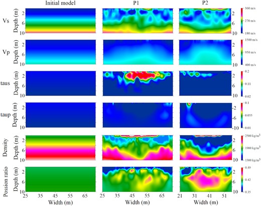
Final models below both profiles obtained by 2-D viscoelastic FWI with the PCG method. The initial models are represented in the first column. The second and third columns represent the reconstruction results of profiles 1 and 2, respectively. Since we only use one relaxation mechanism (Bohlen 2002; Gao et al. 2021), τs and τp are approximated as 2/Qs and 2/Qp where Qs and Qp are the quality factor of S and P waves, respectively.
We show the results of all inverted parameters from both profiles in a 3-D layout (Fig. 11). The cross-sections show a good agreement in the majority of the results. The low S-wave velocity layer with a high Poisson’s ratio delineates the high saturated sandy layer at the depth of 4–6 m. The sudden increase in VP indicates the location of the water level. The log profiles are extracted at the crossing point location and are shown to further evaluate the inverted results (Fig. 12). The final profile indicates that the velocities are the dominant parameters and have high consistency. The final reduced data misfits are shown in Figs 13(a) and (b). We also compare the final synthetic seismogram with the observed data in Figs 13(e) and (f). In both profiles, the synthetic seismogram fits the observed data in satisfactory, indicating a successful data fitting between the observed wavelets by the inverted multiparameter models. The final estimated STFs for every shot in both profiles are shown in Figs 13(e) and (f). We can note that the inverted STFs show a similar shape among each other. It is worth mentioning that the final wavelet does not necessarily represent the actual source wavelet excited in the field surveys, instead, it also accounts for the residual caused by the inaccurate inversion results (Groos et al. 2014).
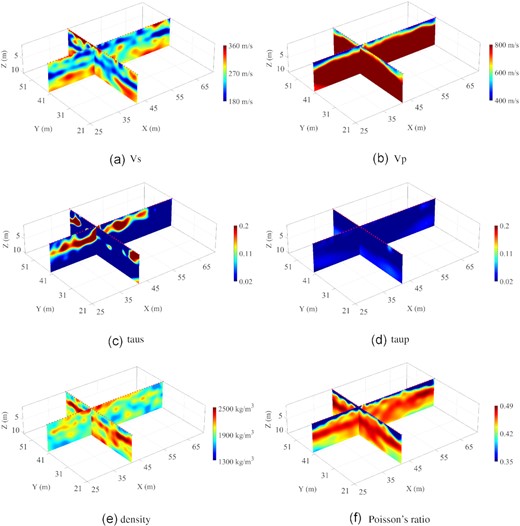
Cross-section of the reconstructed models of both profiles by multiparameter FWI. (a) VS; (b) VP; (c) τs; (d) τp; (e) ρ and (f) Poisson’s ratio. The red triangles represent the receivers.
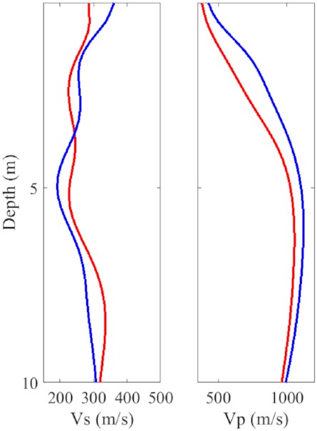
The log extracted from the profile 1 (red solid line) and 2 (blue solid line) at the intersection.
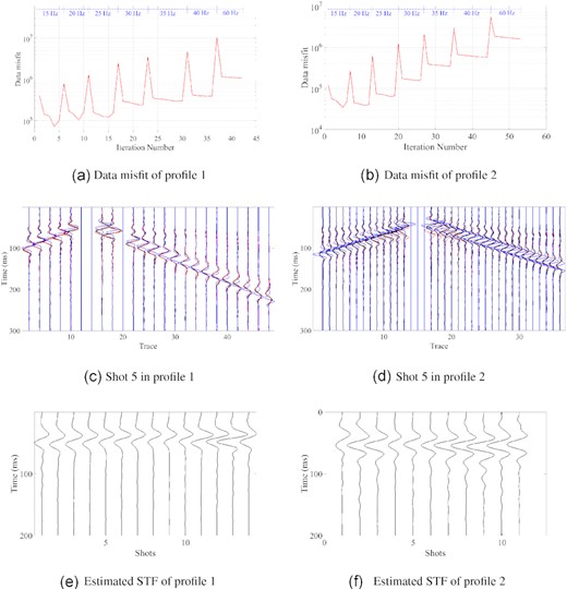
(a) and (b) represent data misfit for P1 and P2, respectively; jumps of increasing misfit value correspond to changes of the FWI workflow stage. (c) and (d) represent the comparison of the trace-normalized observed (black), initial (blue) and synthetic seismograms (red) for shot 5 in P1 and P2, respectively. The shot gather for the shot 5 in profiles 1 is displayed with every second traces. (e) and (f) represent the estimated source time functions of data acquire along P1 and P2, respectively.
5 CLUSTER ANALYSIS
Cluster analysis, as a multivariate statistical method, can be used to correlate and integrate information from a broad range of observations into relatively homogeneous units by dividing the data according to their distances based on the multidimensional parameter spaces instead of a prior information about the classification. K-means algorithm (Macqueen 1967) has been proposed as a useful approach to integrate the useful structural information from multivariate geophysical data. Shallow-seismic wavefields are dominated by the Rayleigh wave, which has a high sensitivity to S-wave velocity. Meanwhile, P-wave velocity and Poisson’s ratio are sensitive to the saturation situation. We applied the K-mean cluster analysis algorithm in three data spaces (VP, VS and ν). As data pre-processings, we normalized the velocity and Poisson’s ratio to assign similar weights before the analysis. In the cluster analysis, the choice of the cluster number is critical. Generally, the number of clusters can be assigned according to the variance ration criterion (VRC, Calinski & Harabasz 1974). Here, according to previous partitions for the GPR inversion results and CPT results, we manually set a cluster number of three in this case (Gueting et al. 2015).
The three clusters are shown in Fig. 14(a). Although the velocity and Poisson’s ratio results in Fig. 9 present the general layered character of the subsurface, however, the correlation of the layers is not clear. According to cluster analysis considers with three data spaces, the spatial distribution of these homogeneous units is shown in Fig. 14(b). Cluster 1 is characterized by higher P-wave velocity, and higher Poisson’s ratio, but with a lower S-wave velocity. Cluster 2 is characterized by lower P-wave velocity, and lower Poisson’s ratio, but with a higher S-wave velocity. Cluster 3 is characterized by an intermediate velocity and Poisson’s ratio. Based on the cluster analysis, the characterization of the subsurface from the seismic data has been integrated into only three-parameter groups and thus the clustered section delineates the major structural feature of the original models.
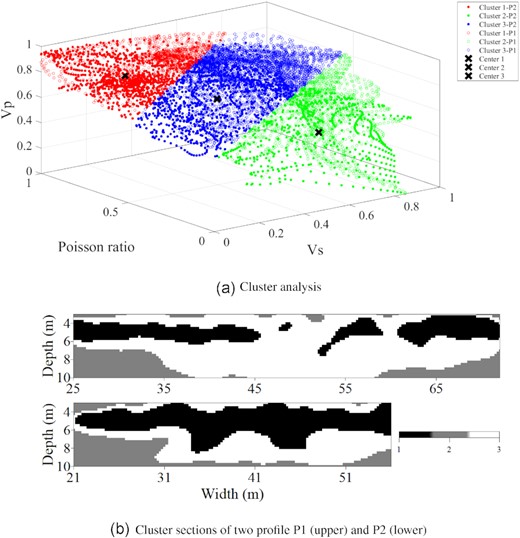
Cluster analysis. (a) The 3-D plot of P-wave velocity, S-wave velocity and Poisson’s ratio. The red, blue and green dots are divided by the K-mean cluster analysis. The crosses delineate three cluster centres. (b) Cluster sections of the two profiles P1 and P2 according to the classification in (a). Numbers and colours refer to specific clusters.
In order to validate our results of cluster analysis of seismic data, we compare the seismic data clusters with the cluster analysis results of CPT data (Gueting et al. 2015) in Fig. 15. The spatial distribution of the clusters shows a nice agreement, especially for the depth of 4–6 m. The distribution of the grain size obtained from borehole B32 (Gueting et al. 2015) indicates that: the CPT cluster 1 corresponds to those materials that the grain size analysis indicates gravel; CPT cluster 2 corresponds to those materials that the analysis indicates sand, and CPT cluster 3 corresponds to those materials that the analysis indicates an intermediate material such as gravelly sand or as sandy gravel. The water content histograms, which are related to porosity also show relatively high porosity from cluster 2, relatively small porosity from cluster 1, and an intermediate porosity from cluster 3, which are corresponded to the relative velocity and Poisson’s ratio’s changes in seismic clusters.

6 CONCLUSIONS
2-D multiparameter viscoelastic FWI of surface waves proved to be a promising tool for the reconstruction of viscoelastic multiparameter models of the shallow subsurface. FWI with Hessian-based optimization method outperforms gradient-based method with higher resolution and fewer ambiguities, which has been verified by using a synthetic example. The exploration scale varies from different fields, however, nearly all the applications are based on the fundamental property of surface waves that it is dispersive. It propagates along the free surface and the longer wavelengths penetrate deeper and are more sensitive to the properties of the deeper layers. While short wavelengths are sensitive to the physical properties of surficial layers. Thus it can also be generalized at lower frequencies for global seismology. We have explored the potential of applying the multiparameter FWI method in the well-studied alluvial aquifer area. It indicates that multiparameter FWI can offer valuable information to offer high-resolution characterization of seismic properties. In addition, the benefit of the parameters attenuation and mass density with information potential in characterization of the alluvial aquifer areas must be investigated further in the future.
The K-mean cluster analysis integrates multivariate seismic inversion results and defines three distinct facies at the Krauthausen test site. The spatial distribution of different classifications in profile 2 presents a nice agreement with the previously defined facies of CPT clusters, which confirms the accuracy of the classified facies. Comparison between the face distribution with the previous analysis indicates that the lithological units may correlate with the variation of the grain size and porosity. Overall, the experiment indicates that the FWI of seismic data can produce high-resolution subsurface models. Combined with the cluster analysis of the multivariate inverted data, FWI could give us an applicable approach to classifying geophysical facies. Integrating other geophysical and geohydrological parameters (e.g. GPR data, grain size and flowmeter data) can help to better characterize the aquifer.
ACKNOWLEDGEMENTS
The authors thank for Editor René-Edouard Plessix and two anonymous reviewer for their constructive suggestions and comments. The authors would also like to thank Martin Pontius, Niko Athanasopoulos and other students attending the Geoverbund ABC-J 2018 Summer School on Hydrogeophysics at Forschungszentrum Jülich for their generous help during the field-data acquisitions. This work was funded by the National Science Foundation of China under grant 42130808, Hubei Provincial Natural Science Foundation of China under grant S22H650101 and the Deutsche Forschungsgemeinschaft (DFG, German Research Foundation), Project ID 258734477-SFB 1173.
DATA AVAILABILITY
The data presented in this study are available upon reasonable request to the first author.
REFERENCES
APPENDIX A
A1 1. Choosing the tolerances
The strategy for choosing the tolerances θn and the maximal inner iteration number kn, max here is set as:
where
and
with the initialization as γ = 0.9 and θmax = 0.999.
A2 2. Additional safeguarding step
To ensure the nonlinear residuals bn = dobs − Φ(m) to be strongly decreasing for monotonicity, enforce it by backtracking as:
Safeguard
 |
|
Safeguard
|
|
APPENDIX B: LINEAR EQUATION CALCULATION
For the self-contentedness of this paper, we recall formulae originally derived by Kirsch & Rieder (2019) and further presented by Gao et al. (2021).
B1 1. Gradient and wavefield calculation
To searching for a GN update, we could solve eq. (7) by linear conjugate gradient. The adjoint |$\phi ^{\prime }(\boldsymbol {m})^\dagger$| at |$\boldsymbol {m}=(\rho ,V_S,\tau _s,V_P,\tau _p)\in \mathcal {M}$| is given by
The detailed explanation of the notations are displayed in Table 1.
B1.1 Right-hand part in eq. (7)
: |$\Phi ^{\prime \dagger }(\Phi (\boldsymbol {m})-\boldsymbol {d}_{obs})$|
For |$\boldsymbol {g}=\Delta \boldsymbol {d}=(\Delta \boldsymbol {v}, \Delta \boldsymbol \sigma _0, \dots , \Delta \boldsymbol \sigma _l)$|, which is the data residual. In this case, |$\boldsymbol {v}$| is the velocity component of the solution of the transformed forward equation (Gao et al. 2021):
|$\boldsymbol {w}$| uniquely solves the backward equation:
with |$\boldsymbol {w}(T)=0$|.
B1.2 Left-hand part in eq. (7)
: |$\Phi ^{\prime \dagger }\Phi ^{\prime }\Delta \boldsymbol {m}$|
It can be explicitly solved with eq. (B1) with |$\boldsymbol \phi ^{\prime }(\boldsymbol {m})\boldsymbol {\hat{m}}=\boldsymbol {\bar{u}}$| where any |$\boldsymbol {\hat{m}}=(\hat{\rho },\hat{v}_s,\hat{\tau }_s,\hat{v}_p,\hat{\tau }_p)\in \mathcal {M}$|, and |$\boldsymbol {\bar{u}}=(\boldsymbol {\bar{v}},\boldsymbol {\bar{\sigma _0}}, \dots , \boldsymbol {\bar{\sigma _L}})$| with |$\boldsymbol {\bar{u}}(0)=0$| is the solution of
where |$(\boldsymbol {v}, \boldsymbol {\sigma _0}, \dots , \boldsymbol {\sigma _L})$| is the solution of eq. (B2).
The coefficients in eq. (B1) are:
with |$\boldsymbol {\Sigma }=\Sigma _{l=1}^{L}\boldsymbol \psi _l$|, |$\mu =\frac{\mu _0}{\rho }$| and |$\pi =\frac{\pi _0}{\rho }$|.
B2 2. Explanation of the notations
Here we display the necessary explanation of the notations used in the FWI algorithm in Table 1.
