


SUMMARY
Although slip inversion has been almost always reported to be inherently non-unique, we prove that Fredholm integral equations of the first kind for slip inversion are mathematically of a unique solution, theoretically assuring that earthquake rupture can be properly reconstructed if there exist a sufficiently large number of measurements. The statement about non-uniqueness of slip inversion can be misleading and misunderstanding, since it is theoretically not true but simply caused by a practical issue of lack of measurements. We propose an inequality-constrained regularized inversion of slip distributions on multiple faults. The method implements a physically more general inequality constraint to accommodate more complex dislocation models and allows reconstructing a complex earthquake mechanism on multiple faults from measurements. The corresponding inequality constraints are a natural extension of positivity constraints proposed by Olson & Apsel and Hartzell & Heaton, or the equivalent inequality constraints that only allow slips to take place between −45° and 45° around the main rupture direction. The regularization parameter is chosen by minimizing the mean squared errors of inverted slip solutions. The proposed method is applied to the 2016 Kumamoto Mw 7.0 earthquake with GNSS measurements. Our slip inversion results show that the 2016 Kumamoto earthquake is only of magnitude Mw 6.7 and ruptures shallowly up to 10 km under the surface. More precisely, about 94 and 88 per cent of the energy released from Hinagu and Futagawa faults take place up to this depth, with the maximum slips of 4.81 and 7.89 m on each fault, respectively.
1 INTRODUCTION
Reconstruction of slip distributions on faults is essential for earthquake engineering and to understand source mechanics of earthquakes (see e.g. Aki & Richards 1980; Lay & Wallace 1995). Slip distributions have often been determined from seismic recordings (Olson & Apsel 1982; Hartzell & Heaton 1983), terrestrial geodetic measurements (Savage & Hastie 1966; Ando 1975; Ward & Barrientos 1986), global navigation satellite systems (GNSS) (Freymueller et al. 1994; Cambiotti et al. 2017) and/or interferometric synthetic aperture radar (InSAR) imaging (Lohman & Barnhart 2010; Yang et al. 2022). These different types of measurements have their own advantages and disadvantages. For example, seismic measurements are much more sensitive than geodetic measurements. Modern seismometers with micro-electro–mechanical systems are required to respond to seismic motion of acceleration at the noise level of 10−5 to
A number of methods can be used for inversion of slip distributions, including least squares (see e.g. Savage & Hastie 1966; Ando 1975; Olson & Apsel 1982; Tarantola & Valette 1982), generalized inverse of matrices (see e.g. Menke 1984; Segall & Harris 1986; Barrientos & Ward 1990), regularization (see e.g. Freymueller et al. 1994; Lohman & Barnhart 2010; Gallovič et al. 2015) and Bayesian inversion (Tarantola 1987; Cambiotti et al. 2017; Benavente et al. 2019). Due to measurement errors and likely model limitations, these inversion methods can result in negative slips that are against the main direction of rupture on a fault, which are believed to be physically not acceptable. To make inversion results of slip distributions physically reasonable, Olson & Apsel (1982) first proposed imposing the positivity constraints on slip components (see also Hartzell & Heaton 1983) and applied the method to study the 1979 Imperial Valley earthquake. The positivity constraints, also referred improperly to as and treated as no-back slip constraints in the seismological literature, have since been widely applied in seismology, in particular, for inversion of slip distributions (see e.g. Du et al. 1992; Courboulex et al. 1997; Cambiotti et al. 2017; Benavente et al. 2019; Ortega-Culaciati et al. 2021), for inversion of moment and slip rates (see e.g. Das & Kostrov 1997; Bindi & Caponnetto 2001; Lindsey et al. 2021) and for determination of source time functions (see e.g. Zollo et al. 1995; Chu et al. 2009; Plourde & Bostock 2017). The positivity constraints for inversion of slip distributions have also been modified to allow slips to take place between −45° and 45° around the main rupture vector on the fault plane (see e.g. Asano & Iwata 2016), which are mathematically equivalent to positivity constraints from the solution point of view. For simplicity, we will refer to these particular inequality constraints as the 45° positivity constraints in the remainder of this paper.
The positivity constraints on slip distributions may imply a physically simplified model of rupture, since the slips of rupture are only allowed to point within a quarter of arc. An earthquake may be physically more complex in terms of a combination of edge, screw and plastic dislocations and can involve multiple faults. From this point of view, we should better not impose too strict constraints to inattentively eliminate such a possible complexity of rupture in advance. Thus, it may be more appropriate to relax the positivity constraints so that we can reconstruct more complex slip distributions on the fault planes of earthquakes from measured data. A reasonable physical assumption would be that no projected component of a slip is permitted to move against the main rupture direction on a fault. As a result of this relaxed assumption, we expect to physically reconstruct and better understand a more complex source of earthquake (if any). In this paper, we will reformulate this relaxed condition as a set of inequality constraints to reconstruct slip distributions. On the other hand, both the positivity constraints and the 45° positivity constraints can only be applied on a single fault. Although they can be applied to an earthquake involved with different faults, this can only be possible, if the main ruptures on all these faults are of the same rake angle, as can be seen in the literature (see e.g. Asano & Iwata 2016; Yue et al. 2017). We will show later in this paper that our new formulation is free of this restriction on the same rake angle and can readily be applied to study a large earthquake with the ruptures taking place on multiple faults with different rake angles. From this point of view, our new approach is theoretically more advantageous. More specifically, we will propose and formulate a new inequality-constrained regularized inversion method in Section 2. We will then simulate examples in Section 3 to demonstrate how the method works and to show the effect of positivity constraints on slip inversion. Finally, we will apply the proposed inversion method to the 2016 Kumamoto Mw 7.0 earthquake with the ruptures on both Hinagu and Futagawa faults from GNSS measurements in Section 4.
2 AN INEQUALITY-CONSTRAINED REGULARIZED SLIP INVERSION METHOD FOR MULTIPLE FAULTS
Before we go on to present our inequality-constrained regularized inversion method, some remarks about existence, uniqueness and stability of inverting slip distributions would be useful and helpful.
Remark 1. Since the integral equation (1) or (2) is physically motivated and mathematically formulated, the existence of solution is warranted. Given the geometry of a fault and the displacement functions on the surface of the semi-infinite elastic medium, the uniqueness of solution should also become clear, as demonstrated in the above. Nevertheless, slip/rupture inversion has often been stated to be inherently non-unique in the seismological literature (see e.g. Olson & Apsel 1982; Olson & Anderson 1988; Das & Kostrov 1994; Beresnov 2003; Mai et al. 2016), a statement of this kind is misleading. Actually, the slip/rupture solution to the integral equation (1) or (2) is mathematically unique. In seismology, what we really encounter is more practical. We can never have all the displacement functions
Remark 2. Seismologists often use a limited number of geodetic/seismic data to compute a much larger number of slip/rupture unknowns. In other words, the total number of geodetic/seismic data is smaller than that of unknown slip components, namely, n < 2t in the case of static slip inversion or at each epoch of sampling in the case of kinematic slip inversion, as can routinely be seen, for example, in Olson & Anderson (1988), Das & Kostrov (1994), Reilinger et al. (2000), Sekiguchi et al. (2000), Bouchon et al. (2002), Custódio & Archuleta (2007), Hao et al. (2017), Hallo & Gallovič (2020) and Asano & Iwata (2021). In this case of n < 2t, the consequences of such a common practice of inversion are straightforward and direct. Different research groups worldwide reported almost completely different slip distributions for the same earthquakes. Two of such examples are the 17 August 1999 Izmit earthquake M 7.5 (compare e.g. Reilinger et al. 2000; Feigl et al. 2002; Gülen et al. 2002; Li et al. 2002; Bouchon et al. 2002; Sekiguchi & Iwata 2002; Delouis et al. 2002; Beresnov 2003) and the 1992 Landers, California earthquake Mw 7.3 (compare e.g. Cohee & Beroza 1994; Freymueller et al. 1994; Wald & Heaton 1994; Cotton & Campillo 1995; Hartzell & Liu 1996; Hernandez et al. 1999; Minson et al. 2013; Xu et al. 2016; Gombert et al. 2018; Wang et al. 2022). In fact, even different types of data and/or different inversion methods have been well known to produce significantly different slip models (see e.g. Olson & Apsel 1982; Feigl et al. 2002). Confusing situations of this kind should clearly indicate that there is still a long way to correctly image what really happens on the fault during an earthquake. Fundamental understanding and correct knowledge of data and inversion methods are critical for properly recovering physical information on slips to advance seismological science or understanding of faulting mechanics.
Remark 3. If n < 2t, the discretized inverse model (5) has an infinite number of mathematically equivalent solutions, which fit the data equally well. No single solution is better than any others in the solution set, as mathematically explained in Xu (1997). There is no extra information to decide which solution should dominate physically either. A common practice in seismology is to obtain a unique solution in this case by applying minimum norm, regularization and/or Bayesian methods to (5). Although the minimum norm, regularization and Bayesian methods can produce a unique solution to (5), they are mathematically equivalent to defining a different mathematical datum for the rank-deficient model (5). However, such a datum is not better than any other constraints mathematically and is not physically justified. Thus, such a unique solution is simply superficially the best. Even worse, since any unique solution to the rank-deficient model (5) contains artificial information, any geophysical interpretation of the solution is very likely biased and not physically supported, which can only add one more element of confusion to slip imaging. We should emphasize that mathematics can only provide a tool to help extract physical information from measurements. It cannot create physical information that does not exist. Incorrect prior assumption behind Bayesian inference is of consequences. We may like to note: (i) Bayesian inference in the geophysical literature always implicitly assumes zero prior mean, which means that we implicitly assume that there are no slips on the fault. Slips do occur on faults during earthquakes. Thus, this implicit assumption of zero prior mean is clearly not true, whose implications have been either mentioned in statistics (see e.g. Akaike 1980) or well addressed in geodesy (see e.g. Xu 1992a, 2021b; Xu & Rummel 1994); (ii) no matter whether the number of data is sufficient, if the prior information used in Bayesian seismology is subjective, the error evaluation of the estimated parameters is not correct either, as demonstrated from the statistical point of view by Xu (1992a, 2021b). The concept of mean squared errors (MSE) should apply; and (iii) a popular opinion exists in the seismological community that Bayesian inference solves this type of problems, since it explores a huge number of candidate models. Such an advantage is superficial as well, in particular, for inverse ill-posed problems. Given a Gaussian random variable, as often used in slip inversion, it is essentially equivalent mathematically to represent this random variable in a probability density, in a set of mean and variance, or in a large number of samplings. The last representation does not have any advantage than the former two representations. In fact, unless the number of samplings is sufficiently large, it is less efficient to report the full information on the random variable.
Based on these remarks, and bearing in mind that the integral equations (1) and (2) are of the first kind and their solutions are inherently very sensitive to small errors of measurements, all what we can do is to find a best balance among a limited number of data, modelling, solution stability and quality (in terms of MSE). If the number of data is small, we should reduce the resolution of slip distributions by increasing the size of patch, no matter whether we like it or not. Let measurements speak for themselves and let them decide to what extent we can extract physical information from a limited number of measurements. Even though the resolution is lowered, at the very least, we are sure that this is the only physical information we can derive from the measurements. It is more realistic and closer to the truth, since it honestly reflects the real situation without use of any subjective or superficial information. It can avoid any potential arbitrary and possibly misleading interpretation of faulting mechanics for earthquakes, due to superficial fine resolution of slips on a fault. Therefore, we will assume n > 2t throughout this work.
3 SYNTHETIC SIMULATED EXAMPLES
The purpose of this section is fourfold: (i) to demonstrate the proposed inequality-constrained inversion of slip distributions; (ii) to show the effect of positivity constraints in the case of a more complex slip distribution on a fault; (iii) to compare the results with the proposed inequality constraints in this paper and those with the positivity constraints and the 45° positivity constraints; and (iv) to show the consequences of an insufficient number of measurements in slip inversion. To make sure that the simulated results are statistically significant and that numerical comparisons are scientifically sound for the first three purposes, we will assume a sufficiently large number of surface displacement measurements, even though we know that the number of geodetic measurements such as GNSS stations is often quite limited in reality. Nevertheless, InSAR indeed could provide us with far more displacement measurements on the surface.
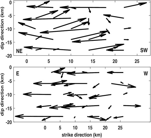
We use Matlab (R2021a, ver.9.10) to simulate a complex slip distribution on a fault (length 44.88 km, width 30.00 km, strike 55.0° and dip 66.0°), which is divided into 7 × 6 patches, though the simulated slip distribution may be apparently different from results of slip inversion in the seismological literature. The true slips simulated on the patches are shown in Fig. 1, which range from 0.14 to 3.56 m in magnitude and from –81.82° to 86.25° in rake, with a mean slip value of 0.97 m and a mean rake angle of 5.42°, respectively. The total release of energy through slips on the fault is equivalent to an earthquake of Mw 7.0. The example is simulated to clearly demonstrate that complex slips cannot be correctly reconstructed and will be precluded, if inversion is not properly constrained, as will be illustrated in the cases of the positivity constraints and the equivalent 45° positivity constraints. Actually, we do not know whether complex slip patterns of this kind can be physically possible/feasible. Thus, it is interesting to see whether the inequality-constrained regularized inversion proposed in this paper can reconstruct such a complex slip distribution.
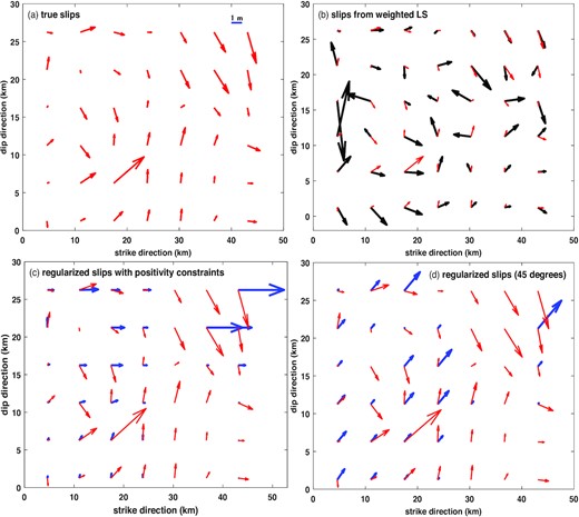
The simulated true slips and the results of slip inversion with a less number of measurements than that of unknown slip components on the fault, computed with the minimum norm weighted LS method and the regularization method with either the positivity constraints or the 45° positivity constraints. Panel (a): the simulated true slips; panel (b): the inverted slips with the minimum norm weighted LS method; panel (c): the inverted slips by applying the regularization method with the positivity constraints; and panel (d): the inverted slips by applying the regularization method with the 45° positivity constraints. For convenience of comparison, we also show the simulated true slips in red in all the other three panels of inverted slip solutions.
3.1 Consequences of slip inversion with an insufficient number of measurements
Many seismological inversions of slip distributions have been carried out with an insufficient number of measurements, as can be seen in, for example, Olson & Anderson (1988), Das & Kostrov (1994), Reilinger et al. (2000), Bouchon et al. (2002), Custódio & Archuleta (2007), Hao et al. (2017) and Hallo & Gallovič (2020). In other words, we will have to invert for more unknown slip parameters from a less number of measurements. In this case, the simplest method is to apply the pseudo-inverse of the normal matrix
For this purpose, we simulate 15 GNSS stations, which are uniformly distributed symmetrically on the surface above the fault in an area of 40 km by 20 km. We then like to invert for 84 slip components on the fault from the 45 components of displacements at these 15 GNSS stations. Since GNSS precise point positioning (PPP) does not require a reference datum and is advantageous for seismological applications, we assume that the displacements from these 15 GNSS stations are all obtained with GNSS PPP. One more important advantage of PPP over the relative GNSS positioning method is that if the latter is used to process GNSS data, we can only obtain the relative displacements for slip inversion, which will theoretically weaken the geometry of measurements, in particular, those important GNSS stations in the epicentre of a large earthquake. As for the random errors of the measured displacements, although PPP has often been reported to be of a few cm accuracy, this level of accuracy is only true to give a statistical image of PPP long-term performance. In seismological applications, we are more concerned with a short term performance of PPP over a few minutes. Xu et al. (2013) reported that the accuracy of PPP over a short period can reach 3–4 mm in the horizontal components and subcentimetre in the vertical component. More theoretical and practical confirmations can be found in Shu et al. (2017) and Xu et al. (2019a,b). Thus, the displacements are simulated with a 4 mm accuracy for the horizontal components and 8 mm for the vertical component. The inversion results of slips on the fault with the minimum norm weighted LS method are shown in Fig. 1, which is equivalent to an earthquake of Mw 7.24. Although the value of moment magnitude is only slightly larger than the true value of Mw 7.00, it is rather clear from the upper-right panel of the figure that the minimum norm weighted LS slips are not physically acceptable in the sense that the slips apparently move arbitrarily around the clock of 24 hr and are significantly different from the simulated true values both in the magnitudes and directions of slips.
Following the standard practice of slip inversion in the seismological community, although there are an insufficient number of measurements, we go ahead by using regularization and/or Bayesian method to determine the optimal regularization parameter as if the unknown parameters
To conclude, if there are an insufficient number of measurements, none of the methods in the above, namely, the minimum norm weighted LS method and the two variants of regularization with either the positivity constraints or the 45° positivity constraints, can correctly reconstruct the complex (true) slip distribution for the simulated example, though the moment magnitudes computed with these results of slips are not very different from the simulated true value Mw 7.00.
3.2 Slip reconstruction with more measurements than the slip unknowns
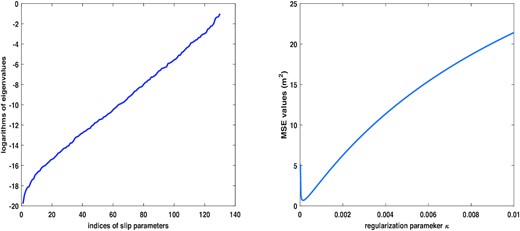
We will now simulate more displacement measurements than necessary to invert for the slip distribution with the new proposed inversion method. In total, we simulate 29 403 displacements in an area of 60 km by 40 km above the fault, with half of them on one side of the strike and the other half on the other side. As in Section 3.1, we will invert for the same 84 slip components on the fault. The simulated standard deviation σ is set to 0.004 m. Although this example is only of 84 slip unknowns to be determined from a very large number of 29 403 displacements, its condition number still reaches a very high value of 3.38E+10, with the smallest eigenvalue of 8.83E-10. The eigenvalues of the example are shown in Fig. 2. To validate the correctness of the forward modelling, we assume no modelling errors and reconstruct the 84 slips with the weighted LS method from the true values of 29 403 displacements, namely, the simulated measurements without adding any random errors, which are shown in the right-hand panel of Fig. 2, together with the true values of slips. It is clear that if the measurements are error-free, the slips are perfectly recovered, with the maximum error of 8.91E-07 m.
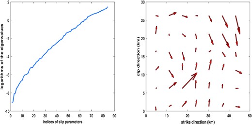
The eigenvalues of the simulated example to reconstruct the slip distribution (left-hand panel) and the weighted LS reconstruction of the slip distribution from the measurements free of random errors (right-hand panel). In this right-hand panel, the slips reconstructed with the weighted LS method from the error-free measurements are shown in black and the simulated true slips in red, which completely overlap each other.
We apply four inversion methods to invert for the slip distribution on the fault, namely, the inequality-constrained regularization method, the minimum norm weighted LS method and the two variants of regularization with either the positivity constraints or the 45° positivity constraints.
Before we discuss the inversion results of slips, we would like to note that the minimum norm weighted LS method and regularization fit the data very well. In fact, they exactly recover the true value of the standard deviation, namely,
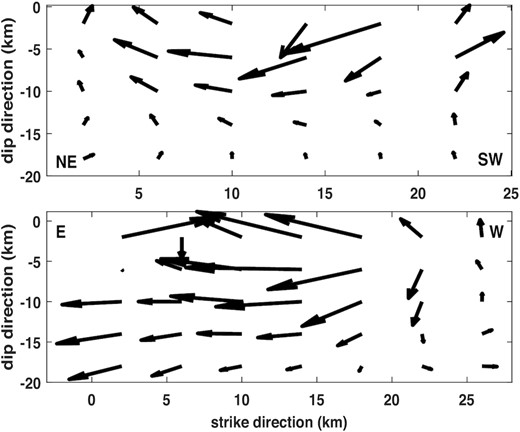
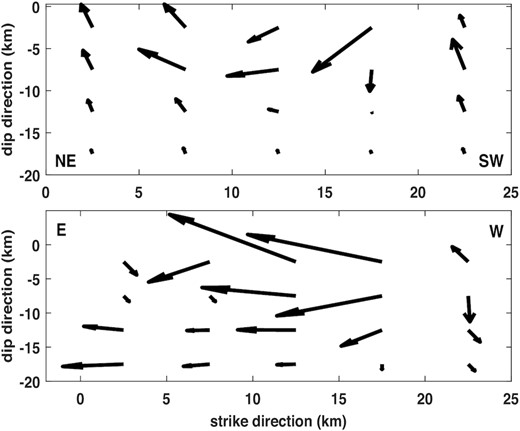
For a detailed analysis and comparison of the four inversion methods, we plot the corresponding reconstructed slip distributions in Fig. 3. Although the minimum norm weighted LS method is well known to lead to unstable and unreliable estimates, we still show its estimated slips here mainly for a quick comparison. It is clear from Fig. 3 that the minimum norm weighted LS method and the two variants of regularization with either the positivity constraints or the 45° positivity constraints result in almost completely incorrect reconstructions of the slip distribution in both sizes and directions of slips. The failure of these three methods is likely due to the fact that the simulated true slip distribution is physically complex. From this point of view, it is not appropriate to impose strong inequality constraints on slip inversion, in particular, since we indeed do not know whether dislocations associated with a certain earthquake are simple or complex. The inequality-constrained regularization method proposed in this paper can be generally said to be very successful to accurately reconstruct the simulated complex slip distribution. Most of the slips on the fault are correctly reconstructed, since the reconstructed and true vectors of slips almost exactly overlap, as can be seen from the lower-right panel. Nevertheless, the largest slip vector has been underestimated.
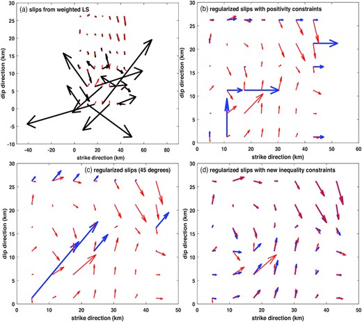
The slips on the fault reconstructed with the minimum norm weighted LS method, the two variants of regularization with either the positivity constraints or the 45° positivity constraints, and our inequality-constrained regularization method. Panel (a): the inverted slips with the minimum norm weighted LS method (black arrows); panel (b): the inverted slips by applying the regularization method with the positivity constraints (blue arrows); panel (c): the inverted slips by applying the regularization method with the 45° positivity constraints (blue arrows); and panel (d): the inverted slips by applying our inequality-constrained regularization method (blue arrows). For convenience of comparison, we also show the simulated true slips in red in all these four panels of inverted slip solutions.
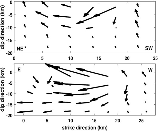
Bearing in mind that the smoothness constraints of derivatives with the Laplacian operator are commonly used in slip inversion, we compute the Laplacian-based smoothness matrix
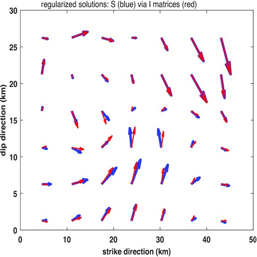
The slip distributions reconstructed by using regularization with the Laplacian-based smoothness matrix
4 APPLICATIONS TO THE 2016 KUMAMOTO MW 7.0 EARTHQUAKE FROM GNSS MEASUREMENTS
A moment magnitude Mw 7.0 earthquake hit Kumamoto, Japan, at 01:25 am in the early morning of 16 April 2016 (Japan local time) according to Japan Meteorological Agency (JMA) (https://www.data.jma.go.jp/svd/eqev/data/2016_04_14_kumamoto/index.html), which involved the two fault systems of Futagawa and Hinagu (see e.g. Asano & Iwata 2016, 2021; Fukahata & Hashimoto 2016; Scott et al. 2019; Hallo & Gallovič 2020). The earthquake was reported to start on Hinagu fault, reach the intersection of Hinagu and Futagawa faults and then continue the rupture onto Futagawa fault (Asano & Iwata 2021). As in the case of all other large earthquakes in Japan, this earthquake was well recorded by the excellent, continuous monitoring seismological infrastructure of Japan such as the strong motion monitoring networks ‘K-NET/KiK-net’ (see e.g. Kinoshita 1998; Aoi et al. 2004, 2020) and the continuous GNSS monitoring network ‘GEONET’ (see e.g. Tsuji et al. 2013; Tsuji & Hatanaka 2018). It was also well mapped by geodetic imaging satellites such as the ALOS-2 satellite and Sentinel-1 satellite (see e.g. Fukahata & Hashimoto 2016; He et al. 2020; Yang et al. 2021).
A number of kinematic and static rupture models for the earthquake have been published with different types of data and different solution methods. These models are derived either purely by using interferometric synthetic aperture radar (InSAR) data from the ALOS-2 satellite (see e.g. Fukahata & Hashimoto 2016; Yang et al. 2021), teleseismic and strong motion data (see e.g. Asano & Iwata 2016, 2021; Yagi et al. 2016; Hao et al. 2017; Hallo & Gallovič 2020), GEONET GPS data (see e.g. Tanaka et al. 2019) or by combining InSAR, GPS, seismic and light-detection-and-ranging (LiDAR) data (see e.g. Yue et al. 2017; Scott et al. 2019; He et al. 2020). Almost all researchers obtained a moment magnitude Mw 7.0 or slightly larger for this earthquake (see e.g. Fukahata & Hashimoto 2016; Yagi et al. 2016; Hao et al. 2017; Yue et al. 2017; Scott et al. 2019; Tanaka et al. 2019; He et al. 2020; Hallo & Gallovič 2020; Yang et al. 2021; Asano & Iwata 2021). The maximum slip can range from about 5 m (see e.g. Fukahata & Hashimoto 2016; Asano & Iwata 2016, 2021; Yang et al. 2021) or about 6 m (see e.g. Yagi et al. 2016; Hao et al. 2017; Tanaka et al. 2019) up to 8 m (see e.g. Hallo & Gallovič 2020) or even 10 m (Yue et al. 2017). In most cases, the maximum slip was reported to take place on Futagawa fault. Nevertheless, inconsistent results were also mentioned by Scott et al. (2019), who reported that LiDAR-optical-InSAR and optical-InSAR inversions ended up with the maximum slip on Hinagu and Futagawa faults, respectively. Overparametrization is obvious in the case of slip inversion with seismic or GPS data. For example, Asano & Iwata (2016) divided Hinagu and Futagawa faults into 189 patches of size 2 km by 2 km, and used only 15 strong motion stations to reconstruct the kinematic rupture process. A further investigation was reported recently by Asano & Iwata (2021) to refine the kinematic rupture process with 220 patches from 20 strong motion stations. Yagi et al. (2016) tried to recover the slip distribution on 290 patches with teleseismic P-wave data at 27 broad-band seismic stations. Hao et al. (2017) used 32 teleseismic and 29 long-period waveforms to invert for slips on 290 patches. Hallo & Gallovič (2020) chose 29 strong motion stations to recover slips on 234 patches. In the synthetic tests, they tried to invert for slips on 720 patches with strong motion data of 40 stations. In the case of GEONET GPS data, Tanaka et al. (2019) determined static slips on 126 patches from only 20 GEONET stations. Positivity constraints are also imposed to avoid physically unacceptable slip solutions (see e.g. Asano & Iwata 2016; Yue et al. 2017; Scott et al. 2019).
A major purpose of this section is to demonstrate our inequality-constrained regularized inversion method with a real example of earthquakes involved with multiple faults. The 2016 Kumamoto Mw 7.0 earthquake with two faults of Hinagu and Futagawa is one of such best examples. So far as data and modelling are concerned, we will limit ourselves to GNSS data and avoid the issue of modelling deficiency of slip inversion in the first instant by directly using a larger size of patch under the reality of a limited number of measurements. Although InSAR could provide many more measurements, the problem is that geodetic InSAR imaging can only repeat itself after almost 1 month in the case of the ALOS-2 satellite (see e.g. He et al. 2020; Yang et al. 2021) or about two weeks in the case of the Sentinel-1A satellite (He et al. 2020). Unless post-seismic slips, major foreshocks and aftershocks are properly taken into account, the factors of these kinds can affect inverted slip distributions of the main shock, because they all contribute to measured displacements due to poor temporal resolution inherent to InSAR. On the other hand, seismic inversion of slip distributions is often underdetermined with more unknowns than measurements (see e.g. Yagi et al. 2016; Asano & Iwata 2016; Hao et al. 2017; Tanaka et al. 2019; Hallo & Gallovič 2020) and (implicitly) requires arbitrary (artificial) information to find a unique solution. Seismometers are also well known to be inherently subject to instrumental drift, tilts and clipping. Even more, accelerograms have been found to be numerically unreliable in the case of high sampling rates and technological innovation of accelerometers is now under development (Xu 2021a). Thus, we will refrain ourselves from using seismic data on this earthquake.
4.1 Fault geometry and test computation
We use Okada’s elastic half-space model to compute displacements by using the Matlab codes of Beauducel (2014), with a Poisson’s ratio of 0.25 and a rigidity modulus of 30 GPa. Before we start the slip inversion, we make several test computations. We first follow Asano & Iwata (2016) and set the length and width of Hinagu fault to 15 and 18 km, and those of Futagawa fault to 27 and 18 km, respectively. The test computation shows that the length of Hinagu fault is somehow too short to accommodate the coseismic displacements of the GEONET stations. As a result, we extend the length of Hinagu fault to 24 km. We should like to note, however, that their slip results tended to satisfy a shorter length for Hinagu fault, while our test computation does require the extension of length from those used, for example, in Asano & Iwata (2016) and Yagi et al. (2016). Our test computation is satisfactory with the length of Futagawa fault used by Asano & Iwata (2016), though other researches used a length of up to about 40 km for this part of the fault (see e.g. Fukahata & Hashimoto 2016; Hao et al. 2017).
The second test computation is to see what resolution of slip inversion may be expected with the GEONET displacements (to be explained later). Although a very fine resolution of 2 km by 2 km patch size has been reported in the literature (see e.g. Yagi et al. 2016; Asano & Iwata 2016; Hao et al. 2017; Hallo & Gallovič 2020), the GEONET stations that can be used to study this earthquake are obviously not sufficient to support this fine resolution of slip inversion without imposing more or less arbitrary and superficial information that cannot be checked independently. We will avoid this situation of having more unknowns than measurements in the first instant. As a result, we start with a patch size of 3 km by 3 km but find that the corresponding formulation is still too ill-posed to handle, since our computer fails to correctly compute the condition number of the normal matrix
As for the parameters of fault geometry, different researchers obtained or used different strike and dip angles for both faults (see e.g. Asano & Iwata 2016, 2021; Fukahata & Hashimoto 2016; Yue et al. 2017; Hao et al. 2017; He et al. 2020; Hallo & Gallovič 2020; Yang et al. 2021). We will just take the reported strike/dip/rake angles from the above publications, compute the average values of these angles and use them as the fault parameters in our inversion of slip distributions. The mean strike, dip and rake angles are equal to 204.33°, 73.82° and –169.68° for Hinagu fault and 233.61°, 65.60° and –158.50° for Futagawa fault, respectively. We select the GEONET data in the Kyushu area but limit ourselves to those stations whose coseismic displacements are statistically significant with a probability of 95 per cent, based on the standard deviations of 0.004 m for the horizontal components and 0.008 m for the vertical component (see e.g. Xu et al. 2013; Shu et al. 2017). We finally have three component ENU displacements at 123 GEONET stations, whose horizontal displacements are shown in Fig. 5, together with the main shock and Hinagu/Futagawa faults. Among these 123 GEONET stations, only 13 stations are of horizontal displacements larger than 0.1 m. The maximum coseismic horizontal displacement is 1.018 m, with the maximum coseismic vertical displacement of 0.251 m at the same GEONET station.
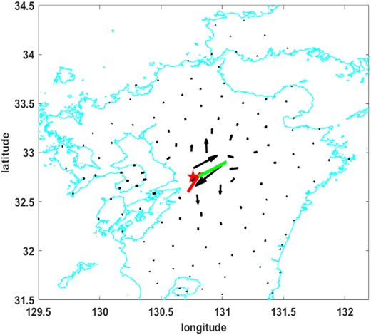
The horizontal displacements at the 123 GEONET stations (black arrows), the JMA epicentre of the 2016 Kumamoto Mw 7.0 earthquake (red star) and the involved Hinagu (red line) and Futagawa (green line) faults. The largest horizontal displacement is 1.018 m.
Using the combined geometry of the specified fault parameters and the 123 GEONET stations, we can readily obtain the coefficient matrix
The eigenvalues of the slip inversion with a patch size of 4 km by 4 km (left-hand panel) and the MSE values with different values of regularization parameter κ (right-hand panel).
4.2 Inversion results of slip distributions
The regularized reconstructions of slip distributions on Hinagu and Futagawa faults without imposing the physical inequality-constraints (8) are shown in Fig. 7, which are equivalent to an earthquake magnitude Mw 7.1. The basic features of both slip patterns on Hinagu and Futagawa faults are that large ruptures take place shallowly at the depth less than 10 km. This is particularly true on Hinagu fault up to a few km beneath the surface. Nevertheless, it is clear that because the inversion of slips is highly ill-posed with a very large condition number, the naïve regularized inversion results in some unreasonable slips, in particular, in the southwest end of Hinagu fault and roughly right under Aso volcano in the eastern end of Futagawa fault, as can be seen in Fig. 7. Thus, we apply the inequality-constrained regularization to invert for the static slips, which are plotted in Fig. 8 and are equivalent to an earthquake magnitude Mw 6.6. Our moment magnitude Mw 6.6 is slightly smaller than almost all other researches (see e.g. Yagi et al. 2016; Asano & Iwata 2016, 2021; Fukahata & Hashimoto 2016; Yue et al. 2017; Hao et al. 2017; He et al. 2020; Hallo & Gallovič 2020; Yang et al. 2021). The physically constrained regularized slips in Fig. 8 remain the basic feature of rupture that major ruptures take place shallowly on both Hinagu and Futagawa faults. All the physically unreasonable slips disappear on both faults. The largest slips are 4.11 m on Hinagu fault and 6.93 m on Futagawa fault, respectively; both of them take place less than 5 km in depth under the surface. More precisely, about 82 and 78 per cent of energy are released by the large ruptures taking place up to about 8 km right below the surface on Hinagu and Futagawa faults, respectively, which will readily generate large horizontal displacements on the surface. These results may be highly related to and explain well the largest damage of Mashiki city roughly at the corner of intersection of Hinagu and Futagawa faults (see e.g. Kawase et al. 2017), even though we only obtain a moment magnitude Mw 6.6 for the 2016 Kumamoto earthquake. we may like to note that the 45° positivity constraints result in about the same magnitude Mw 6.6 but with apparently unacceptable slip distributions, which are shown in Fig. S1 in the electronic supplementary materials.
The regularized reconstructions of static slips on Hinagu (upper panel) and Futagawa (lower panel) faults with a patch size of 4 km by 4 km.
The inequality-constrained regularized solutions of static slips on Hinagu (upper panel) and Futagawa (lower panel) faults with a patch size of 4 km by 4 km. The maximum slips on Hinagu and Futagawa faults are 4.11 and 6.93 m, respectively.
To show the effect of regularization parameter κ on slip inversion, we increase the regularization parameter from its optimal value 1.5296E-04 to 0.01. In this case, the condition number is sufficiently small, implying that we can readily obtain a stable inversion of slips. The inverted slip distributions derived from the regularized reconstructions without and with the inequality-constraints (8) are shown in Figs S2 and S3, respectively. The regularized slips are equivalent to a moment magnitude Mw 6.8. It is clear by comparing these two figures that all the ruptures slip along almost the same direction on both Hinagu and Futagawa faults, no matter whether the inequality-constraints (8) are applied. Nevertheless, at the very least, a closer look has consistently shown that about 76 and 79 per cent of energy release take place shallowly up to less than 10 km under the surface on Hinagu and Futagawa faults. We should point out, however, that the reconstructions of slips with the regularization parameter 0.01 are oversmoothed and largely biased, as can be seen from the MSE values on the right-hand panel of Fig. 6.
To further demonstrate the importance of physical inequality constraints, we now show the slip distribution in Fig. 9, which is obtained by applying regularization only with the Laplacian smoothness matrix
The regularized solutions of static slips on Hinagu (upper panel) and Futagawa (lower panel) faults with the Laplacian smoothness matrix
Up to the present, we have not touched too much on the data fitting. The reasons are threefold: (i) good fitting of data does not mean good solutions for inverse ill-posed problems, as mentioned in Remark 3. The weighted LS solution is an extreme example, which attains the best fitting of data but is the least accurate and almost always physically meaningless; (ii) the most important and most difficult aspect of inverse ill-posed problem theory is to accurately reconstruct the unknown function of interest; and (iii) it is clear from (12) or (13) that the basic objective function of all regularization methods is involved with two terms: one responsible for data fitting and the other for regularization. Unless the regularization parameter κ is incorrectly selected, regularization methods and the weighted LS method would generally result in a similar performance of data fitting. Nevertheless, since people seem to care much about data fitting in seismic inversion, we plot the original GEONET horizontal displacements in Figs S4–S7, together with their LS and regularized counterparts with different regularization methods. As theoretically expected, the data fittings from different regularization methods in this paper are not very different.
Since the measured GEONET displacements, the weighted LS estimates and their corresponding regularized displacements almost overlap each other in Figs S4 and S6, we further locally amplify the large displacements in the epicentre area and show the data fitting for each of the weighted LS and regularization methods in Figs S5 and S7. We can intuitively see from the panels in Figs S5 and S7 that the weighted LS method fits the data best, as theoretically expected. The regularization method without any constraints performs better than that with our new inequality constraints. The method with the 45° constraints is of the worst performance of data fitting. For more details, the reader is referred to the electronic supplementary materials.
Bearing in mind that a patch size of 4 km by 4 km leads to a very large condition number of 5.9219E+18, we would like to investigate the effect of patch size on slip inversion by increasing the patch size to 5 km by 5 km. In this case, we only have 40 patches, or more precisely, 20 patches on Hinagu fault and another 20 patches on Futagawa fault. The eigenvalues of the normal matrix
The 5 km by 5 km patch size leads to the optimal regularization parameter of 1.5960E-04, which is basically the same as in the case of 4 km by 4 km patch size. The regularized model with the 5 km by 5 km patch size fits the GEONET displacements with a fitting error of 0.0229 m, which is slightly better than that of 0.0258 m with the 4 km by 4 km patch size. The inequality-constrained regularized reconstructions of slips are shown in Fig. 10, with an equivalent moment magnitude Mw 6.7. Comparing the inverted slips on both Figs 8 and 10, we can find that the feature of major rupture in the very shallow parts of Hinagu and Futagawa faults remains unchanged, with the maximum slips of 4.81 and 7.89 m on Hinagu and Futagawa faults, respectively. More precisely, about 94 and 88 per cent of the energy release from the rupture on each of Hinagu and Futagawa faults take place up to the depth of 10 km, respectively; this may again be highly related to the largest damage observed in Mashiki town. The maximum slip of 4.81 m on Hinagu fault is much larger than most researches on the earthquake but may still be reasonable. Actually, Scott et al. (2019) even found the largest slip on Hinagu fault from the LiDAR-optical-InSAR data. The inversion results with the 5 km by 5 km patch size may be more preferable in terms of a smaller fitting error and model simplicity, in particular, bearing in mind that the number of the GEONET stations with a sufficient large displacement in Kyushu area is limited to study this earthquake.
The inequality-constrained regularized solutions of static slips on Hinagu (upper panel) and Futagawa (lower panel) faults with a patch size of 5 km by 5 km. The maximum slips on Hinagu and Futagawa faults are 4.81 and 7.89 m, respectively.
Based on the reconstructed slip distributions in Figs 7–10, we may like to summarize that: (i) due to the limited data with a weak geometrical constraint on the fault slips, the regularized slip results without the inequality constraints can be physically unreasonable; (ii) because of a very large condition number with only the GNSS displacements, we could likely only be able to obtain the basic pattern of slip distributions on Hinagu and Futagawa faults. The detailed results of slips, in particular, those right under the Aso volcano in the eastern part of Futagawa fault, may very likely be unreliable and inaccurate, again, due to a very large condition number, or equivalently, the weak geometrical constraint of the limited number of GNSS data. Any geophysical interpretation of the detailed results of slips should be exercised with great care; and (iii) it is hard to judge whether the slight reverse components on both Hinagu and Futagawa faults could be real in terms of the very large condition number, though the inequality-constrained regularized slip distributions fit the vertical GNSS displacements well. We obtain a small fitting error of 0.005 m for the largest vertical displacement of 0.251 m. With the largest vertical uplift displacement of 0.251 m near the Futagawa fault in mind, such slight reverse components might be physically possible to help release the earthquake energy with a very severe rupture in the very shallow parts of the faults. A slight reverse component can also be observed on Hinagu fault from InSAR (Hallo and Gallovič 2020; Yang et al. 2021) and on Futagawa fault from InSAR (compare the left part of slip inversion results of figs 4 and 6 in Fukahata & Hashimoto 2016). Nevertheless, even if InSAR data are used, different researchers could obtain inconsistent results about the possibility of a slight reverse component, as can be inferred by comparing fig. 8 in Yang et al. (2021) with fig. 6 in Fukahata & Hashimoto (2016).
5 CONCLUSION
Slip inversion is essential to understand source mechanics of earthquakes. Problems of inverting for static and/or kinematic rupture from surface measurements have been almost always stated to be inherently non-unique in the seismological literature (see e.g. Olson & Apsel 1982; Olson & Anderson 1988; Das & Kostrov 1994; Beresnov 2003; Mai et al. 2016). Statements of this kind mathematically imply that slip/rupture could have never been correctly recovered, because there exist an infinite number of mathematically equivalent solutions to any problem that is inherently non-unique, irrelevant of whether we would have an infinite number of geometrically best possible measurements on any earthquake. Given the geometry of a fault and the displacement functions on the surface of the semi-infinite elastic medium, the slip function on the fault is defined by Fredholm integral equation (1) or (2) of the first kind. We prove that Fredholm integral equation (1) or (2) of the first kind for slip inversion is mathematically of a unique solution, which is a theoretical guarantee that earthquake slip/rupture can be properly reconstructed if there exist a sufficiently large number of measurements. The non-uniqueness issue of slip inversion in the seismological literature is not mathematically true but is practically caused due to lack of measurements. This practical aspect of non-uniqueness due to lack of data should not be overemphasized to avoid any potential misunderstanding that reconstructing the slip distribution on a fault could never be possible, physically and mathematically.
We have proposed an inequality-constrained regularized inversion of slip distributions on multiple faults. The method implements physically more general inequality constraints to accept more complex dislocation models and/or a combination of complex dislocation models. The formulation of constraints (8) is theoretically significant in three aspects: (i) it mathematically allows the reconstruction of more complex slip/rupture of an earthquake (if any) from measurements; (ii) it can be applied to a large earthquake involving multiple faults with different rake angles; and (iii) the corresponding inequality constraints (8) can be thought of as a natural extension of the positivity constraints, or equivalently, the 45° positivity constraints, as first proposed by Olson & Apsel (1982) and Hartzell & Heaton (1983) for a single fault or multiple faults with a single rake angle. The regularization parameter is chosen by minimizing the mean squared errors of the inverted slip solution.
The proposed method is applied to the 2016 Kumamoto Mw 7.0 earthquake with GNSS measurements. We have limited the number of patches to avoid the rank-deficiency (or non-uniqueness) of the linearized version (5) of Fredholm integral equation (1) or (2) of the first kind due to lack of data in the first instant, since a rank-deficient linear system of equations can only produce a set of mathematically equivalent solutions with an infinite number of elements. Although the number of GEONET stations in the study area allows a maximum number of about 180 patches for both Hinagu and Futagawa faults, test computations have shown that with a patch size of 3 km by 3 km, the model (5) is extremely ill-conditioned. Physically reasonable solutions could hardly be expected. Therefore, we have focused on investigating two patch sizes, namely, one with the size of 4 km by 4 km and the other with the size of 5 km by 5 km. The inequality-constrained regularized inversions with both sizes of patches have resulted in a similar pattern of slip distributions on both Hinagu and Futagawa faults. The ruptures of the earthquake take place shallowly up to 10 km under the surface of Hinagu and Futagawa faults. The inverted slips with the patch size of 5 km by 5 km are preferable in terms of model simplicity and a smaller fitting error, and since there are only a limited number of GEONET displacements larger than 10 cm. The inversion results of slips have shown that: (i) the 2016 Kumamoto earthquake is only of magnitude Mw 6.6-6.7. Nevertheless, if the inequality constraints are not imposed on the slips of Hinagu and Futagawa faults, namely, slips are allowed to move freely around the clock, then the seismic moment magnitude we obtained for the 2016 Kumamoto earthquake is equal to Mw 7.13 with a patch size of 4 km by 4 km (or Mw 7.16 with a patch size of 5 km by 5 km), which is comparable with what has been reported in the literature, though physically apparently not feasible; and (ii) about 80–94 percent of the energy release takes place up to the depth of 10 km or even shallower on Hinagu and Futagawa faults, with the maximum slips of 4.11–4.81 m on Hinagu fault and 6.93–7.89 m on Futagawa fault, respectively, which may be highly related to the largest damage in Mashiki town observed by Kawase et al. (2017).
Finally, we may also like to note that obtaining a unique solution to a rank-deficient linearized model due to lack of data could not make us closer to the truth of an earthquake, since such a unique solution involves subjective or artificial information. We can never know whether such artificial information is correct or not. Instead, it is highly recommended to use a rougher patch in this case, which may seemingly prevent us from a fine (but arbitrary) imaging of an earthquake; but at the very least, we could get some more or less close-to-true information on the earthquake. Much more effort should be made to advance seismological infrastructures, in particular, innovations of seismometers and space geodesy imaging, for more useful and real-time data on large earthquakes.
SUPPORTING INFORMATION
Figure S1. The regularized slip distributions with the 45° positivity constraints: the upper panel—Hinagu fault; the lower panel—Futagawa fault.
Figure S2. The regularized slip distributions with a 0.01 regularization parameter without the inequality-constraints: the upper panel—Hinagu fault; the lower panel—Futagawa fault.
Figure S3. The regularized slip distributions with a 0.01 regularization parameter with the inequality-constraints: the upper panel—Hinagu fault; the lower panel—Futagawa fault.
Figure S4. The horizontal displacements at the 123 GEONET stations (black arrows), their weighted LS estimates (red arrows), the estimates regularized respectively with the 45° positivity constraints (cyan arrows) and our own new inequality constraints (green arrows) and the ordinary regularized estimates without inequality constraints (blue arrows). The largest horizontal displacement is 1.018 m.
Figure S5. The GEONET horizontal displacements, the weighted LS estimates and the regularized estimates with the identity smoothness matrix shown inside the box with red dashed line in Fig. S4. Panel A: the GEONET displacements (black arrows) and the weighted LS estimates (red arrows); panel B: the GEONET displacements (black arrows) and the regularized estimates (blue arrows); panel C: the GEONET displacements (black arrows) and the regularized estimates with the 45° positivity constraints (cyan arrows); and panel D: the GEONET displacements (black arrows) and the regularized estimates with our own new inequality constraints (green arrows). The largest GEONET horizontal displacement is 1.018 m.
Figure S6. The horizontal displacements at the 123 GEONET stations (black arrows), the estimates regularized, respectively, with the 45° positivity constraints (cyan arrows) and our own new inequality constraints (green arrows) and the ordinary regularized estimates without inequality constraints (blue arrows). The largest horizontal displacement is 1.018 m. This figure is different from Fig. S4 in that the Laplacian smoothness matrix is implemented in regularization instead of an identity smoothness matrix.
Figure S7. The horizontal displacements and the regularized estimates with the Laplacian smoothness matrix shown inside the box with red dashed line in Fig. S6. Panel A: the GEONET displacements (black arrows) and the regularized estimates without any constraints (blue arrows); panel B: the GEONET displacements (black arrows) and the regularized estimates with the 45° positivity constraints (cyan arrows); and panel C: the GEONET displacements (black arrows) and the regularized estimates with our own new inequality constraints (green arrows).
Figure S8. The eigenvalues of the slip inversion with a patch size of 5 km by 5 km (left-hand panel) and the MSE values with different values of regularization parameter k (right-hand panel).
Please note: Oxford University Press is not responsible for the content or functionality of any supporting materials supplied by the authors. Any queries (other than missing material) should be directed to the corresponding author for the paper.
ACKNOWLEDGEMENTS
I thank Prof K. Heki for suggesting making Figs S4 and S6 more reader-friendly, which results in two more locally amplified figures, namely, Figs S5 and S7. I also thank an anonymous reviewer very much for the constructive comments, which have helped improve the manuscript.
DATA AVAILABILITY
I acknowledge the Geospatial Information Authority (GSI) of Japan for the GEONET displacement data and thank Prof Y. Fukahata very much for making the data available to me. Hinagu and Futagawa faults are shown on the basis of the active fault bank in Japan at the link https://gbank.gsj.jp/activefault/search.
