


SUMMARY
Understanding water redistribution on Earth's surface is essential to hydrological applications and water management. Variations in water mass loads have been observed by the Gravity Recovery and Climate Experiment (GRACE), but the low spatial resolution of GRACE limits determination of their distribution in detail. Hydrologic models provide higher spatial resolution water mass loads, but may include larger uncertainties. In this study, we develop high-resolution surface mass loads over the Amazon basin using forward modelling by combining GRACE data and a hydrologic model. River routing discharge is also included as a priori information because of the large water volume changes on relatively narrow channels in the Amazon basin. These high-resolution surface mass loads constrained by river routing agree with GRACE observations when spatially smoothed. Vertical deformation estimated from these high-resolution loads agree with Global Navigation Satellite System (GNSS) observations, at both seasonal and inter-annual timescales. In particular the most improved agreement is obtained at the NAUS GNSS station, close to the main channel of the Amazon, relative to predictions made using GRACE data. At two other stations (APSA and MAPA) near the main channel, the estimated vertical deformations apparently differ from observation, but much of the discrepancy is reduced when river path is corrected in river-routing model, indicating the importance of water loads on river channel to understand crustal displacement in the area.
1 INTRODUCTION
Accurate and detailed monitoring of water mass distribution on land is essential for understanding and predicting climate change that may be related to ongoing global warming. According to the recent IPCC AR6 (IPCC 2021), the climate has warmed significantly regionally and globally during the last century, and resulting climate changes provoke extreme droughts and floods more frequently. Consequently, accurate measurements of water mass distribution are required to anticipate and prepare for corresponding natural disasters (Eltahir & Bras 1996; Mishra & Singh 2011). Despite its importance, knowledge of water distribution has been limited due to lack of in-situ measurements, particularly in remote areas (IPCC 2021).
Water mass distribution on land can be estimated by hydrological models. These models use observational analyses and atmospheric model re-analyses to provide global land surface states and fluxes with high spatial resolutions (≤ 1°, Rodell et al. 2004; Dee et al. 2011; Rui & Beaudoing 2015). In hydrological models, terrestrial water storage can be determined by time-integration of water fluxes across the Earth's surface (Rui & Beaudoing 2015). However, they tend to be uncertain because changes in water storage are relatively small compared with large water fluxes such as precipitation or evaporation. In addition, most hydrological models do not account for water mass transported in river channels which is one of main components in water redistribution (Dill et al. 2018).
Since 2002 May, the Gravity Recovery and Climate Experiment (GRACE) mission has provided monthly gravity solutions (Bettadpur 2004; Tapley et al. 2004). Gravity changes during a one-month interval are mainly caused by water storage variations on land after correcting for atmospheric and dynamic ocean signals. These time-varying gravity solutions are converted into terrestrial water mass distribution with global coverage (Wahr et al. 1998). However, relatively poor spatial resolution, about 300–400 km (Tapley et al. 2004), remains a limitation of hydrological applications of GRACE (Zhong et al. 2021a;b).
Variations in terrestrial water storage from hydrological models or GRACE can be compared with observations of Earth's surface displacement. Water mass on Earth's surface acts as a load and induces crustal displacement observable by Global Navigation Satellite System (GNSS, Wu et al. 2003; van Dam et al. 2007; Blewitt et al. 2016; Hammond et al. 2016; Han 2016; Yan et al. 2016). Permanent GNSS stations have provided continuous time-series of displacements at annual and inter-annual timescales largely associated with terrestrial water storage. Annual amplitudes range from a few millimetres to several tens of millimetres (Dixon 1991; Blewitt et al. 2001; van Dam et al. 2001). Load displacements at GNSS stations can then be compared with those predicted using hydrological models or GRACE observations assuming an elastic response of Earth's surface to loading mass (Longman 1962; Farrell 1972). Model predictions generally explain GNSS observations, but some inconsistencies have been found (van Dam & Wahr 1987; Wu et al. 2003; Davis et al. 2004; Fu et al. 2013). In many cases these are thought to be largely due to uncertainties in hydrologic (land surface) models, especially in regions where observations of surface and groundwater variations are sparse and models are poorly constrained. In addition, most land surface models do not account for water load variations in river channels, where much of the load may be concentrated (Dill et al. 2018). Therefore, one might expect relatively large disagreement between GNSS observations and hydrologic predictions in regions with both sparse observations and large variations in river channel storage, such as the Amazon basin (Bevis et al. 2005).
GRACE predictions of vertical displacement are highly correlated with GNSS observations. A number of studies have found generally good agreement between predictions from GRACE and GNSS observations in Europe (Wang et al. 2016), North America (Argus et al. 2014), South America (Davis et al. 2004; Ferreira et al. 2019; Fang et al. 2021), Australia (Han 2016; Han 2017) and South Asia (Chanard et al. 2014). However, in the Amazon basin where the largest river in the world is located, the agreement is only reasonable for stations distant from river channels (Tregoning et al. 2009; Fu et al. 2013; Moreira et al. 2016). Amplitudes of GRACE predictions were much smaller than those of GNSS observations close to river channels (Dill & Dobslaw 2013; Moreira et al. 2016; Ferreira et al. 2019). Knowles et al. (2020) reported that the underestimation is mainly at semi-annual and annual timescales, suggesting that the cause may be varying water loads in narrow river channels not resolved by the low spatial resolution of GRACE. Dill & Dobslaw (2013) found that displacements estimated from high-resolution hydrologic models incorporating river routing showed improved agreement with GNSS observations, but discrepancies remained, due likely to limitations of hydrologic models. These results suggest that further progress, particularly near Amazon river channels, may be achieved by combining GRACE and hydrologic model predictions (Chen et al. 2005; Han et al. 2010; Dill et al. 2018; Ndehedehe & Ferreira 2020; Nicolas et al. 2021; Zhong et al. 2021b).
In this study, we estimate surface water mass fields of the Amazon basin at high spatial resolution (0.5° grids) using GRACE observations and hydrological models. Low-resolution GRACE surface mass loads are complemented by high-resolution hydrologic model mass loads. GRACE observations are useful to constrain models where observations may be sparse. We develop an iterative forward modelling (FM) algorithm based on the methodology of Chen et al. (2013) in which a river routing model provides an a priori spatial mass distribution. This is appropriate for the Amazon basin where river channels are an important hydrological component (Pellet et al. 2021a;b). We find that this approach leads to good agreement with GNSS vertical displacement observations. This suggests that surface mass loads combining GRACE and hydrological models should be important hybrid data sets supporting hydrological and geodetic studies.
2 DATA AND METHODS
2.1 GRACE
We used GRACE GSM Release 06 monthly solutions from 2003 January to 2016 August, provided by the Center for Space Research (CSR), University of Texas at Austin (Bettadpur 2018). The GSM solutions consist of spherical harmonic (SH) coefficients up to degree and order 60. SH coefficients at degree-1 (C10, C11 and S11) are not observed by GRACE, while C20 coefficients are inaccurate. Since omission or inaccuracy of these low-degree SH coefficients will cause uncertainties in surface mass loads, we estimated them using higher degree GRACE SH coefficients (Kim et al. 2019) based on an improved version of the method of Sun et al. (2016). Postglacial rebound (PGR) effects are removed using the ICE-6G_D PGR model (Peltier et al. 2018).
GRACE data errors include north–south stripes and high-frequency noise. The DDK filter can be used to suppress them simultaneously (Kusche 2007; Kusche et al. 2009). However, in this study, we removed north–south stripes and high-frequency noise using, respectively, de-striping (Swenson & Wahr 2006) and 400-km Gaussian smoothing (Wahr et al. 1998). In the iterative FM procedure Gaussian filtering is necessary (see Section 2.3 below), leaving GRACE mass field spatial resolution at about 300–400 km (approximately 3°–4° grid spacing).
We also used GRACE RL06 mass concentration (MASCON) solution v02 (Save 2020), provided by CSR (http://www2.csr.utexas.edu/grace). They represent surface mass change with high spatial resolution (0.25° grids), although nominal resolution is 1° (Save et al. 2016). High-resolution MASCON solutions may provide improved spatial resolution of surface mass changes relative to filtered GRACE data (Save et al. 2016). MASCONs include ocean bottom pressure contributions realized in the Atmosphere and Ocean De-aliasing Level-1B (AOD1B) products (Bettadpur 2018) used in GRACE data processing (Save et al. 2016). We used the GAD products to remove monthly means of AOD1B over the oceans.
2.2 Initial mass fields with river flow
Constraints on flow velocity are derived from in-situ data available via ORE_HYBAM (http://www.so-hybam.org). ORE_HYBAM provides water level and discharge data for 97 sites in the Amazon basin from 2000 January 1 to 2017 December 31. We first divided the Amazon basin into 97 sub-basins based on locations of ORE_HYBAM stations. In-situ stations are located at those sub-basins’ mouths except for the lowest sub-basin where in-situ data are not available. Grid cells in the sub-basin are assumed to share the same flow velocity, u. By applying eq. (1) to a sub-basin, we calculate |${q}_{\mathrm{ out}}$| of a grid cell. Varying u, we find the value required to produce |${q}_{\mathrm{ out}}$| that best agrees with in-situ discharge data from ORE_HYBAM. For the lowest sub-basin, we set flow velocity to increase at a rate of 13 cm s−1 per 1° length (Han et al. 2010). Seasonally varying flow velocities would be useful for more realistic discharge estimates, but they are difficult to determine. We simply used constant flow velocities during the study period. Variations of water mass flow along Amazon river channels estimated this way were similar to those observed from GRACE (Han et al. 2010). The river network system is digitized by Total Runoff Integrating Pathways (TRIP, Oki et al. 1999) to connect all grid cells in the domain. Because TRIP is provided at 0.5° resolution, we resampled both surface runoff and soil moisture fields of GLDAS CLM at 0.5° before applying the continuity equation. Locations of several erroneous confluence connections in TRIP were manually adjusted (within a grid cell of 0.5° spacing) to be close to actual river paths using satellite imagery of Google Earth maps with 30 m spatial resolution (https://earth.google.com). The sum of water mass flowing along channels and stored in soil layers within a grid cell was set as the initial state of surface mass loads for the FM algorithm (Fig. 1a). Other models (GLDAS Noah, VIC and Mosaic, Rodell et al. 2004) were also tested, but CLM water discharge showed the best agreement with the in-situ data from ORE_HYBAM (see Fig. S1, Supporting Informaion, for details).
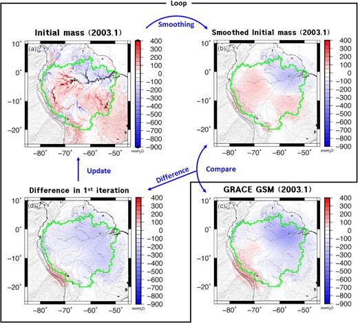
An overview of the forward modelling process (in clockwise order from upper left) using the mass distribution map of 2003 January as an example. (a) High-resolution initial mass redistribution model from routing results and GLDAS CLM soil moisture. (b) Smoothed and localized mass redistribution model from initial mass from (a). (c) GRACE GSM surface mass distribution map to estimate differences compared to (b). (d) The difference between (b) and (c). The FM algorithm updates the differences map (d) to the previous mass field of (a). The process is repeated until the difference becomes negligible.
2.3 Forward modelling
We estimated high-resolution surface mass loads over the Amazon basin using an FM algorithm developed by Chen et al. (2013). The algorithm iteratively adjusts initial mass fields to agree with GRACE observation. The main benefit of FM is to suppress spatial leakage of mass change signals resulting from a limited range of SH coefficients. As described in detail below, we revised the FM algorithm to improve spatial resolution.
Step 1. Gridded initial mass fields with 0.5° spatial sampling from the numerical models (described in Section 2.2) are created. These are converted to SH coefficients up to degree and order 60 and smoothed by the 400 km Gaussian filter described earlier. The de-striping filter is not necessary because the initial mass loads do not include north–south stripes.
Step 2. Smoothed SH coefficients of initial mass fields (from Step 1) are localized to the Amazon basin using Slepian functions (Wieczorek & Simons 2005). Slepian functions are an optimal orthonormal band-limited basis from a linear combination of SHs used to represent scalar quantities on a sphere within a limited area (Slepian 1983). We constructed Slepian functions for the Amazon basin mask (0.5° grid interval) using the first 45 bases localized to the region according to the Shannon criteria which is determined based on the size of the Amazon basin and the maximum SH degree (60). Details are given by Wieczorek & Simons (2005). This localization is necessary to restrict FM to the Amazon basin. Using the Slepian functions, we estimated localized surface mass loads at gridpoints (0.5° grid interval) within the Amazon.
Step 3. Filtered GRACE GSM SH coefficients (the observed mass signals as reference values in FM) are also localized using the same Slepian functions (from Step 2) and surface mass loads at gridpoints within the Amazon are estimated (0.5° grid interval). The difference between the two localized fields [smoothed mass loads from GRACE (Fig. 1c) and the smoothed initial mass load (Fig. 1b) from Step 2] are added to the initial mass field (Fig. 1a).
The FM process repeatedly updates the initial mass field until the solution converges. Converged FM solutions are accepted when the basin-wide RMS difference between two successive FM outputs is less than 0.01 mm (water layer equivalent), approximately 1000 times smaller than GRACE uncertainty. This convergence implies that FM solutions when smoothed agree with the reduced GRACE data within 0.01 mm (Fig. S2, Supporting Information).
Alternatively, we also used the smoothed GRACE data (after de-striping and Gaussian filtering) as an initial mass field for conventional FM, as done in previous studies (Chen et al. 2013; Chen et al. 2015; Ni et al. 2017; Jeon et al. 2018). This also leads to converged mass distributions (Fig. S3, Supporting Information) that effectively suppress signal leakage out of a basin, but spatial resolution of water mass loads within the basin is poor, similar to that of GRACE data (Kim et al. 2019). Comparison of the two different FM solutions (using numerical model output vs. smoothed GRACE data as a priori initial mass loads) is useful to examine the improvement of spatial resolution provided by FM when incorporating hydrologic model information.
2.4 GNSS
GNSS observations of surface displacement are used to verify the accuracy of the FM results. GNSS data were obtained from the Nevada Geodetic Laboratory (NGL), which processes raw data from more than 19 000 stations world-wide, and distributes time-series of daily position at each station (Blewitt et al. 2018). Data are available through the NGL portal website (http://geodesy.unr.edu). We selected 18 permanent stations in the Amazon basin (see Fig. S4 and Table S1, Supporting Information). Time-series of those selected stations are longer than 5-yr with some intermittent missing periods. Mean values of formal error over the 18 stations are about 3 mm vertically and about 1 mm horizontally. We removed daily outliers outside 3σ intervals relative to least-squares fitting of a linear trend and seasonal cycle to GNSS observations. We adjusted abrupt offsets in each residual series (probably due to equipment replacement or earthquakes) using Database of Potential Step Discontinuities from the NGL website (http://geodesy.unr.edu/NGLStationPages/steps.txt). We calculated 7-d average displacements before and after step days and adjust time-series using displacement differences. Then monthly averages of daily time-series were computed to compare with monthly GRACE data. Daily ocean load tides, which vary by more than several millimetres at some stations (Fu et al. 2012), have been corrected during GNSS processing by NGL (Blewitt 2020). In any case, monthly averaging would be expected to suppress ocean load tide signals. The effects of non-tidal atmospheric and ocean loading still remain in the GNSS data and will be considered in GNSS data analysis in the next section. Finally, we subtracted a linear trend to remove tectonic signals from observed displacements.
2.5 Crustal displacements
Using eqs (2)–(4), we estimated displacements from the de-striping and Gaussian smoothing filtered GSM SH coefficients up to degree and order 60. We refer to these displacements as ‘Low-GRACE’. Surface displacements from our high-resolution FM results were calculated after converting to SH coefficients to degree and order 359, approximately the SH Nyquist degree (|${l}_{\mathrm{ max}} \approx {\rm{the\ number\ of\ latitude\ grids}} - 1$|) (Wieczorek & Meschede 2018). FM results provide water loads only within the Amazon basin, but loads outside the basin contribute to additional displacements. We used residual GSM fields, which are the filtered GSM fields with Slepian localized fields subtracted, for the mass load outside of the basin. Surface displacements estimated from conventional FM using smoothed GRACE data as initial mass loads are called ‘FM1’, while those from the revised FM algorithm using high-resolution initial fields (based on hydrological and river routing model) are referred to as ‘FM2’. Additionally, we consider surface displacements associated with non-tidal atmospheric and ocean bottom pressure that were removed from GRACE solutions (Bettadpur 2004, 2018). These are available as GAC solutions from the GRACE data centers (Bettadpur 2018), and we included their contribution in the three displacement estimates (Low-GRACE, FM1 and FM2).
Since MASCONs are on 0.25° grids, surface displacements can be calculated to higher SH degrees. We converted MASCONs into SH coefficients to degree and order 719 and calculated surface displacements using eqs (2)–(4). Contributions from ocean dynamics and atmospheric pressure were added using GAC fields as in the other three estimates. MASCON displacement predictions are called ‘Mascon’.
3 RESULTS
3.1 Surface water mass distribution
We first visually examine four different surface mass load fields. Figs 2(a)–(d) show water mass redistribution over the Amazon basin for 2003 January from filtered GSM, MASCON and the two FM results. Residual GSM fields, which are filtered GSM fields with Slepian localized fields removed, are added to both the conventional and the revised FMs to account for mass loads outside of the basin. The filtered GRACE GSM fields show low spatial resolution (Fig. 2a), with mass loads unable to distinguish Amazon river channels. MASCON (Fig. 2b) and conventional FM incorporating smoothed GRACE data as a priori mass loads (Fig. 2c) show that mass changes are concentrated near mid- and upstream river areas, when compared with filtered GRACE data (Fig. 2a), but have relatively poor spatial resolution. In addition, the three mass load maps show smoothed negative and positive anomalies over east and west parts of the basin, respectively. This dipole pattern covering the whole basin broadly is likely due to regional surface mass anomalies over the basin. Similar dipole patterns are also found in the revised FM using the numerical model outputs of soil moisture and water on river channels as an initial mass field (Fig. 2d), but much smaller scale anomalies are concentrated around channels. Such localized anomalies are only apparent in surface mass load fields from the revised FM.
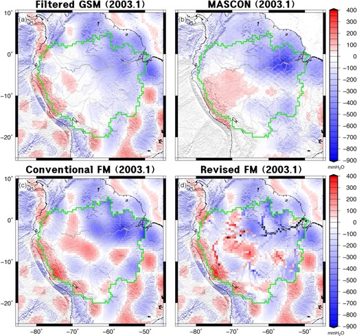
Water mass maps at 2003 January in the Amazon basin from filtered (a) GSM, (b) MASCON, (c) conventional FM and (d) revised FM.
3.2 Vertical displacements
Using eq. (2), water mass loads shown in Figs 2(a)–(d) were used to calculate vertical displacements in Figs 3(a)–(d). In general, four vertical displacement predictions (Low-GRACE, Mascon, FM1 and FM2) show similar spatial patterns even though water mass loads shown in Fig. 2 are evidently different from one another. This is because vertical displacement at a gridpoint is affected by surface mass loads surrounding the point, so that small spatial scale load variations are not evident in vertical displacement fields. That is, vertical load deformation at a point is effectively a smoothed version of nearby mass loading. Nonetheless, at regions close to main river channel stems, the four predicted vertical displacements show distinctive patterns. Low-GRACE near the main channel shows minor uplift anomalies (Fig. 3a). In Mascon and FM1 (Figs 3b and c, respectively), larger surface uplifts are shown around the main stem relative to Low-GRACE, but localized patterns along the main stem are not clear. On the other hand, FM2 (Fig. 3d) shows vertical displacements confined largely to the periphery of the main stem. This indicates that vertical displacements near river channels should be useful to examine relative accuracy of Low-GRACE, Mascon, FM1 and FM2.
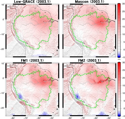
Vertical displacements calculated by surface mass loads shown in Fig. 2.
Predictions of the four surface mass load estimates can be compared with vertical displacements at GNSS stations to judge their relative accuracy. Four vertical displacements (Low-GRACE, Mascon, FM1 and FM2) are compared with observations at 18 GNSS permanent stations in the Amazon Basin (Fig. S5, Supporting Information). We also calculated RMS differences between observed and estimated vertical displacements for all 18 stations (see Table S2, Supporting Information). In general, there is agreement among the four surface mass load predictions of vertical displacement. This was expected given similar vertical displacement maps in Fig. 3. At two stations, MAPA and APSA, however, RMS differences for FM2 are much larger than those from Mascon and FM1. Differences at MAPA and APSA are found to be related to river routing model parameters, as discussed below. Vertical displacements at the two stations are re-examined after addressing this issue.
We also analyse annual amplitudes and phases of observed and estimated vertical displacements for 16 stations. Sinusoids are fit by least squares excluding data from MAPA and APSA. Table 1 shows mean of RMS differences between observations and estimates for annual amplitude and phase at each station. All predictions show similar phase lags (6–8 d), and amplitude differences for Mascon, FM1 and FM2 are similar to each other but slightly smaller than Low-GRACE. As expected from Fig. 3, this shows similar vertical displacements at most GNSS stations distributed over the Amazon from Mascon, FM1 and FM2.
RMS of annual amplitude (mm) and phase lag (day) differences in vertical displacements between GNSS and various load estimates (Low-GRACE, Mascon, FM1 and FM2) for 16 stations (excluding APSA and MAPA). The average annual amplitude in GNSS observations is 13.99 mm.
| Low-GRACE | Mascon | FM1 | FM2 | |
|---|---|---|---|---|
| Amplitude (mm) | 4.20 | 2.45 | 2.33 | 2.24 |
| Phase (d) | 6.46 | 7.94 | 6.41 | 7.29 |
| Low-GRACE | Mascon | FM1 | FM2 | |
|---|---|---|---|---|
| Amplitude (mm) | 4.20 | 2.45 | 2.33 | 2.24 |
| Phase (d) | 6.46 | 7.94 | 6.41 | 7.29 |
However, at NAUS station near the main channel (within 7 km of the channel), RMS values of Low-GRACE significantly differ from those of others (Mascon, FM1 and FM2). Fig. 4(a) shows vertical displacements of Low-GRACE (blue line), Mascon (green), FM1 (yellow) and FM2 (red) at NAUS from 2003 January to 2016 August. Differences between these predictions from the GNSS time-series (dashed black line) are shown in Fig. 4(b). The GNSS observations provide time-series since 2006 January, with missing observations in 2011 December. The seasonal cycle is evident in the GNSS series with an amplitude near 29 mm, and inter-annual fluctuations are also present. Low-GRACE predictions show similarity in phase, but have much smaller amplitudes (∼17 mm) and less inter-annual variability than GNSS. The small amplitudes in Low-GRACE predictions were found in other studies (Dill & Dobslaw 2013; Moreira et al. 2016; Ferreira et al. 2019), likely a result of spatial leakage (smoothing) of localized loads at river channels into areas distant from the channels (Knowles et al. 2020).
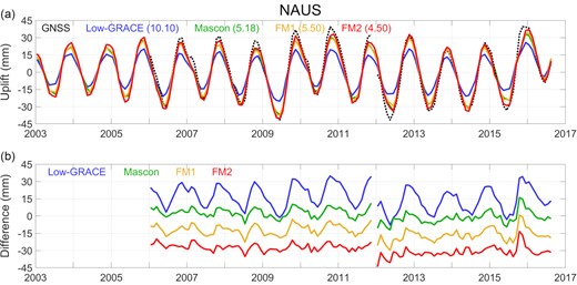
(a) Time-series of vertical displacements observed by GNSS at the NAUS station with time intervals of 1-month (dashed black) and coloured curves representing variations in the loading prediction derived from Low-GRACE (blue), Mascon (green), FM1 (yellow) and FM2 (red). Numbers in parentheses indicates RMS differences between GNSS observations and predictions. Units are mm. (b) Differences between the GNSS observations and the predictions are shown with offset for clarity (same colours with Fig. 4a). Each curve has been offset by 15 mm.
Mascon, FM1 and FM2 predictions are much closer to GNSS observation at the NAUS station. RMS differences associated with FM1 and Mascon are 5.50 and 5.18 mm, respectively, smaller than for Low-GRACE (10.10 mm). In particular, FM2 shows the smallest RMS difference (4.50 mm) among all the predictions. This is because the mass loads from FM2 are more concentrated along river channels than others as shown in Figs 2 and 3. This result indicates an improved understanding of terrestrial water storage with higher spatial resolution from FM using river routing information to obtain FM2.
Relative agreement between GNSS and various predictions of vertical displacements can be clearly seen in a scatter plot (Fig. 5). Fig. 5 for station NAUS shows a linear regression line with slope given at the bottom right of the figure. A slope nearer to unity implies better agreement with GNSS observations. The Low-GRACE slope is smallest (0.57 ± 0.02), as expected from its low spatial resolution. The FM2 slope of 0.92 ± 0.03 indicates good agreement with GNSS. Mascon and FM1 slopes are smaller (0.83 ± 0.03 and 0.82 ± 0.03, respectively) as expected because mass loadings on river channels are not corrected (Save et al. 2016; Karegar et al. 2018; Zhang et al. 2019) as in the case of FM2.
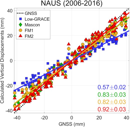
Scatter plots of observed versus estimated vertical displacements from Low-GRACE (blue square), Mascon (green diamond), FM1 (yellow circle) and FM2 (red triangle) at the NAUS station for 2006–2016. Dashed black line has a slope of 1. Numbers at bottom right are slopes.
FM2 slopes, excluding APSA and MAPA, are generally closer to unity than other load estimates in Table 2. In particular, at LSTM near the Amazon main stem (like NAUS), the FM2 regression slope is much closer to unity than other predictions. Other stations near river channels (e.g. LAFL, ROGM and SAGA) show similar results. FM1 is also better than other estimates, but provides smaller slopes than FM2 since FM1 does not provide mass loads concentrated in river channels. At stations distant from river channels (e.g. LRBR, RIOB, ROCD and ROJI), all four predictions yield similar regression slopes. This clearly shows the importance of high spatial resolution load estimates near river channels in predictions of crustal displacements. The mean regression slope over 16 stations (excluding APSA and MAPA) between FM2 and GNSS observations is close to unity (0.91 ± 0.06). Mean slopes for the others (Low-GRACE, Mascon and FM1) are 0.78 ± 0.06, 0.81 ± 0.06 and 0.86 ± 0.05, respectively. Although regression slopes of FM2 are closer to unity than others, similar improvement is not found in RMS differences as shown in Table S2 (Supporting Information). This imply that our new FM2 not only provides surface mass loads in higher resolution than conventional GRACE estimates but also is likely contaminated by additional sources of error possibly from estimates of soil moisture and river runoff from numerical models used as an a priori in FM2.
Regression line slopes from scatter plots for GNSS vertical displacement observations and estimates for 18 stations.
| Station | Low-GRACE | Mascon | FM1 | FM2 | |
|---|---|---|---|---|---|
| 1 | APSA | 0.88 ± 0.09 | 0.96 ± 0.10 | 0.99 ± 0.11 | 1.48 ± 0.13 |
| 2 | BOAV | 0.66 ± 0.07 | 0.63 ± 0.06 | 0.70 ± 0.07 | 0.77 ± 0.07 |
| 3 | CRUZ | 0.69 ± 0.16 | 0.68 ± 0.16 | 0.77 ± 0.17 | 0.74 ± 0.16 |
| 4 | LAFL | 0.93 ± 0.12 | 0.90 ± 0.13 | 0.98 ± 0.14 | 0.99 ± 0.14 |
| 5 | LPMO | 0.60 ± 0.09 | 0.57 ± 0.09 | 0.64 ± 0.10 | 0.67 ± 0.11 |
| 6 | LRBR | 0.94 ± 0.13 | 0.92 ± 0.13 | 1.00 ± 0.14 | 0.96 ± 0.13 |
| 7 | LSTM | 0.55 ± 0.04 | 0.67 ± 0.05 | 0.70 ± 0.05 | 1.12 ± 0.08 |
| 8 | MAPA | 0.92 ± 0.09 | 1.02 ± 0.09 | 1.05 ± 0.09 | 1.53 ± 0.14 |
| 9 | MTCO | 0.89 ± 0.06 | 0.91 ± 0.06 | 0.98 ± 0.06 | 0.98 ± 0.07 |
| 10 | MTSR | 0.81 ± 0.08 | 0.85 ± 0.09 | 0.89 ± 0.10 | 0.88 ± 0.10 |
| 11 | NAUS | 0.57 ± 0.02 | 0.83 ± 0.03 | 0.82 ± 0.03 | 0.92 ± 0.03 |
| 12 | PAAT | 0.79 ± 0.07 | 0.89 ± 0.08 | 0.96 ± 0.09 | 0.84 ± 0.08 |
| 13 | POVE | 0.93 ± 0.04 | 0.96 ± 0.04 | 0.97 ± 0.04 | 0.95 ± 0.04 |
| 14 | RIOB | 0.91 ± 0.07 | 0.89 ± 0.06 | 0.96 ± 0.07 | 0.91 ± 0.07 |
| 15 | ROCD | 0.81 ± 0.05 | 0.84 ± 0.06 | 0.83 ± 0.06 | 0.82 ± 0.06 |
| 16 | ROGM | 0.76 ± 0.05 | 0.82 ± 0.05 | 0.83 ± 0.05 | 1.06 ± 0.08 |
| 17 | ROJI | 0.89 ± 0.10 | 0.89 ± 0.11 | 0.88 ± 0.10 | 0.85 ± 0.10 |
| 18 | SAGA | 0.78 ± 0.07 | 0.75 ± 0.07 | 0.81 ± 0.08 | 1.04 ± 0.09 |
3.3 Horizontal displacements
We examined horizontal displacements using the same methods as for vertical. Dashed black curve in Fig. 6(a) show GNSS observations of N-S displacements at NAUS, and Fig. 6(b) shows the E-W component. In general, horizontal displacements are smaller than vertical. Elastic loading theory predicts that (depending on load distance) horizontal displacements are expected to have amplitudes of 30–50 per cent of vertical (Wahr et al. 2013). The N-S component shows a clear annual variation with amplitude near 4 mm (Fig. 6a) while seasonality in the E-W component is less obvious. The difference is related to the azimuth of seasonal load variations. Seasonal loads affecting NAUS are dominantly Negro and Solimões rivers, south of the station. This creates a seasonal signal on N-S and vertical components, with little effect on E-W.
Comparison of observed and calculated horizontal displacements at NAUS. (a) and (b) are northward and eastward components, respectively. Same colour scheme as in Fig. 4.
We compare GNSS horizontal variations with predictions from various surface loads using eqs (3) and (4). Fig. S6 (Supporting Information) shows time-series of horizontal displacements at all stations. For N-S components, predictions show annual variations in-phase with GNSS (Fig. 6a), but agreement between predictions and observations is relatively poorer than for the vertical component (Fig. 4). Even less agreement is found for E-W components (Fig. 6b). Tables S3 and S4 (Supporting Information) summarize RMS differences between various predictions and observation for N-S and E-W components, respectively. Tables S5 (Supporting Information) (N-S) and S6 (E-W) show regression slopes between predictions and observation. Similar levels of agreement are found for most predictions, although FM2 performs somewhat better than others.
The improved performance of FM2 is also summarized by a box plot which shows the average trend of the regression lines at the 16 stations except MAPA and APSA stations (Fig. 7). The coloured lines indicate the mean values for Low-GRACE (blue), Mascon (green), FM1 (yellow) and FM2 (red). The grey boxes represent the 95 per cent confidence interval while error bars mark the maximum and minimum trends. The average trends for vertical displacement ranges from 0.78 to 0.91. For horizontal displacements (N-S and E-W), the averages are in the range between 0.21 and 0.29, and the maximum and minimum values show a very wide range (from −0.12 to 0.72). Overall, FM2 shows better ratios in both vertical (0.91 ± 0.06) and horizontal (0.29 ± 0.11 for N-S and 0.28 ± 0.11 for E-W) displacements than other estimates.
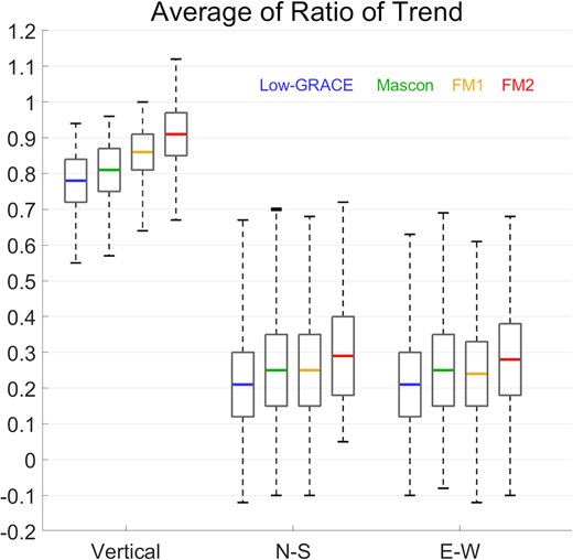
Box plot of the regression line slopes of observed versus estimated displacements at the 16 stations (excluding APSA and MAPA). Coloured lines represent the average of regression line slopes from Low-GRACE (blue), Mascon (green), FM1 (yellow) and FM2 (red), respectively. The grey boxes and black solid lines are 95 per cent confidence intervals and maximum and minimum slopes, respectively.
The relatively large discrepancy in horizontal displacements is likely because they depend on both distance and azimuth to mass loading. The river routing model has half-degree resolution but this appears to be insufficiently precise for the task of predicting horizontal deformation. With generally smaller horizontal amplitudes there is relatively poor agreement between predictions and GNSS observations. Higher resolution load models would be expected to have improved performance.
4 DISCUSSION
FM2 predicts vertical displacements at MAPA and APSA that are larger than observed. The choice of river routing parameters in the model near the river mouth is the apparent cause. Two parameters that affect water load variations are grid cell runoff velocity (Han et al. 2010) and river path (Dill & Dobslaw 2013). There is no gauge station nearby, so it is not possible to use in-situ observations to constrain runoff velocity, but if we vary it over the range 0.7–2.5 m s−1, half to three times the initial value (Han et al. 2010), resulting river channel loads and displacements change only slightly (RMS differences below 0.2 mm).
The routing model river path near the lower reaches of Amazon where MAPA and APSA are located does not accurately represent the actual path. Fig. 8(a) shows a map of the lower reaches of the Amazon river basin from OpenStreetMap (https://www.openstreetmap.org/#map = 8/-0.288/-52.239). The Amazon River (light blue) delivers water to the ocean towards the northeast via several 100 + km-wide braided channels. However, the routing model simulates water flow using only a single channel with 0.5° grid width (blue box and red arrow) near MAPA and APSA, creating a concentrated load that would lead to large predicted amplitudes in Table 2. We modified the model to include multiple river paths in the lower river reach (Fig. 8b). The grid cells corresponding to the main stem in the routing model are extended in north–south direction to fit the actual river channel, and water is evenly distributed over the modified cells (dashed red box). We repeated the forward modelling process as in Section 2 using the modified model.
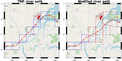
(a) Map of the Amazon river mouth from OpenStreetMap (https://www.openstreetmap.org/#map=8/-0.288/-52.239). The red inverted triangles show locations of MAPA and APSA GNSS stations. Actual river channels of Amazon outfall (light blue) differ that in the TRIP routing model (blue box and red arrow). (b) Modified river routing near the basin mouth to consider multiple river channels. Grid cells of the routing path are extended latitudinally (dashed red box), and routed water is distributed equally over the modified cells.
Fig. 9 shows predicted vertical displacements of original (red) and modified model (cyan) of FM2 at MAPA station. The modified model reduces predicted annual amplitude from 17.56 to 12.66 mm, and the RMS difference decreases from 7.20 to 4.41 mm. The slope of the regression line shown in Table 2 drops from 1.53 ± 0.14 to 1.12 ± 0.10. At APSA a similar improvement is found using the modified model. RMS difference decreases from 6.20 to 3.94 mm, and the regression line slope is reduced from 1.48 ± 0.13 to 1.09 ± 0.11. Improved agreement between predictions and observations at MAPA and APSA demonstrates the importance of detailed understanding of initial mass distribution based on routing model when constructing high-resolution mass redistributions.
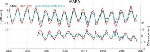
Time-series of vertical displacements observed by GNSS at MAPA with time intervals of 1-month (dashed black). The red line is the original FM2 prediction, and the cyan line shows the prediction after modification of the river model routing path.
5 CONCLUSIONS
Water mass distribution and variations in the Amazon basin are not observed in detail by GRACE alone. Important water mass loads along channels are unresolved by GRACE spatial resolution. Conventional FM or Mascon GRACE solutions improve somewhat the observability of large signals along narrow river channels, but lack the fine scale resolution needed for typical channel sizes. This is evidently the cause of GRACE underestimates of water mass loads at river channels leading to disagreement with vertical displacement observations at GNSS stations.
In this study, we used a modified iterative FM algorithm to adjust GRACE observations to yield water mass distribution in the Amazon basin with a spatial resolution of 0.5°. Our FM approach utilizes a river routing model as a priori to resolve water mass flow in the channels. We found that at most GNSS stations, FM predictions (FM2) well explain vertical displacement observations over the basin, confirming the effectiveness of combining GRACE and a hydrologic model with river routing. The overestimates of FM2 at the two lowest reach stations, MAPA and APSA, are evidently associated with details of the river path, corrected using a modified river path based on a finer-resolution map.
An advantage of our FM approach is that it can be readily extended to other regions such as the Congo, Orinoco and Yangtze basins where water mass variations in river channels are significant. The only requirement is that hydrological models and corresponding river routing in the regions are available to provide reasonable prior estimates. The main limitation of our new water mass loads data in high resolution would be additional uncertainties associated with numerical model outputs used as initial surface mass loads. However, we expect accuracy of model predictions would be also improved from this combined estimates with numerical model and geodetic observation. This refinement of the FM method will be important for other hydrological studies as it provides water distribution maps with enhanced spatial resolution.
SUPPORTING INFORMATION
Figure S1. Water discharge observations from ORE_HYBAM (black line) and its estimations based on GLDAS Noah (blue), GLDAS CLM (red), GLDAS VIC (green), GLDAS Mosaic (yellow) at Óbidos station. Numbers in parentheses indicate RMS differences between the observations and estimations. Similar comparisons were also performed at other 96 sites of ORE_HYBAM in Amazon basin. Overall, the estimated discharge from GLDAS CLM agrees the most with the in-situ data.
Figure S2. Comparison between the revised FM and GRACE GSM surface mass loads at 2003 January. (a) Surface mass loads from the revised FM in the Amazon basin. (b) Smoothed surface mass loads of (a). (c) Smoothed GRACE GSM surface mass loads. (d) Difference between (b) and (c). Surface mass loads from the FM is almost identical to GRACE GSM when they are smoothed.
Figure S3. Comparison between the conventional FM and GRACE GSM surface mass loads at 2003 January. (a) Surface mass loads from the conventional FM in the Amazon basin. (b) Smoothed surface mass loads of (a). (c) Smoothed GRACE GSM surface mass loads. (d) Difference between (b) and (c). Surface mass loads from the FM is almost identical to GRACE GSM when they are smoothed.
Figure S4. 18 permanent GNSS stations used in this study. The red inverted triangles are locations of GNSS stations with identifier codes listed in Table S1. Pairs of two codes separated by commas indicate two nearby GNSS stations whose locations could not be distinguished in this map. Shown in green is the Amazon basin boundary from TRIP (Oki et al. 1999), and its main tributaries including the Amazon River are delineated with black lines. The square outlines the river mouth region shown in Fig. S7.
Figure S5. Comparison of vertical displacements observed by GNSS (dashed black lines, left-hand axis) and predicted by Low-GRACE (blue), Mascon (green), FM1 (yellow) and FM2 (red) at all stations as shown in Fig. 4. Differences between these predictions from the observations are shown in the lower part for clarity (same colours, right-hand axis). Numbers in parentheses indicates RMS differences between the observations and predictions. Units are mm.
Figure S6. Comparison of horizontal displacements observed by GNSS (dashed black lines) as predicted by Low-GRACE (blue), Mascon (green), FM1 (yellow) and FM2 (red) at all stations as shown in Fig. 6. (a) and (b) are N-S and E-W, respectively. Numbers in parentheses indicates RMS differences between observations and predictions. Units are mm.
Table S1. Coordinates of the GNSS stations.
Table S2. RMS differences (mm) in vertical displacements of various estimates (Low-GRACE, Mascon, FM1 and FM2) versus the GNSS observation at the stations.
Table S3. RMS differences (mm) in N-S displacements for various estimates (Low-GRACE, Mascon, FM1 and FM2) versus the GNSS observation at the stations.
Table S4. RMS differences (mm) in E-W displacements for various estimates (Low-GRACE, Mascon, FM1 and FM2) versus the GNSS observation at the stations.
Table S5. Slopes of regression lines between predicted N-S displacements and GNSS observations at 18 stations.
Table S6. Slopes of regression lines between predicted E-W displacements and GNSS observations at 18 stations.
Please note: Oxford University Press is not responsible for the content or functionality of any supporting materials supplied by the authors. Any queries (other than missing material) should be directed to the corresponding author for the paper.
ACKNOWLEDGEMENTS
This study was supported by a research grant from the Korean Ministry of Oceans and Fisheries (Grant no. KIMST20190361) and by the National Research Foundation of Korea (NRF) grant funded by the Korea government (MSIT, Grant nos. 2018R1C1B5086283, 2020R1A2C2006857 and 2021R1F1A1061854). SO was supported by the Nuclear Safety Research Program through the Korea Foundation of Nuclear Safety (KoFONS), granted financial resource from the Nuclear Safety and Security Commission (NSSC), Republic of Korea (Grant no. 1705010). JC was supported by the NASA GRACE and GRACE Follow-On Projects (under grant no. 80NSSC20K0820, contract no. NNL14AA00C and JPL subcontract no. 1478584) and NASA Earth Surface and Interior Program (Grant nos. NNX12AM86G and NNX17AG96G).
DATA AVAILABILITY
The data used in this study are available from a data storage of Open Science Framework (https://doi.org/10.17605/OSF.IO/4JXHT).
