


SUMMARY
Many natural hazards exhibit inverse power-law scaling of frequency and event size, or an exponential scaling of event magnitude (m) on a logarithmic scale, for example the Gutenberg–Richter law for earthquakes, with probability density function p(m) ∼ 10−bm. We derive an analytic expression for the bias that arises in the maximum likelihood estimate of b as a function of the dynamic range r. The theory predicts the observed evolution of the modal value of mean magnitude in multiple random samples of synthetic catalogues at different r, including the bias to high b at low r and the observed trend to an asymptotic limit with no bias. The situation is more complicated for a single sample in real catalogues due to their heterogeneity, magnitude uncertainty and the true b-value being unknown. The results explain why the likelihood of large events and the associated hazard is often underestimated in small catalogues with low dynamic range, for example in some studies of volcanic and induced seismicity.
1 INTRODUCTION
Here, we present a new theory for the convergence of the b-value obtained from eq. (3), based on random sampling of the mean magnitude |$\bar{m}$| with respect to the number of events n and the dynamic range r of observations for the case of an exponential FMD for a randomly sampled finite sample. As an intermediary step, we use a maximum likelihood solution for the modal value in the mean magnitude obtained from a random sample of n events, and obtain the same result as Ogata & Yamashina (1986), who used the expectation value in their derivation. The dynamic range is the difference between the largest observed magnitude ω and mc and is inherently linked to, but not proportionately correlated with the sample size n, with an additional degree of freedom due to the random sampling rather than a one to one correlation assumed in the theoretical curves we show later. Dynamic range is important in its own right because it defines the useful scale of observations, and the extent to which models can be tested in competition with one another. In many applications in seismology, dynamic range is restricted in practice to a relatively narrow range, particularly for volcanic and induced seismicity. We then derive the consequent convergence of the Aki-estimated b-value, denoted bAki, as a function of n and r. We test this model against randomly sampled catalogues with known underlying parameters, and against real data. We find the theory matches the observations well, and hence can be used to estimate the associated bias to high b-values in the common situation where the number of events and the dynamic range are small. This correction is important because high b-values result in an underestimation of the extrapolated likelihood of events larger than ω. In principle, the results could be applied in a similar way to other hazards with power-law frequency-size distributions that can be expressed in the form of eq. (1).
2 THEORY
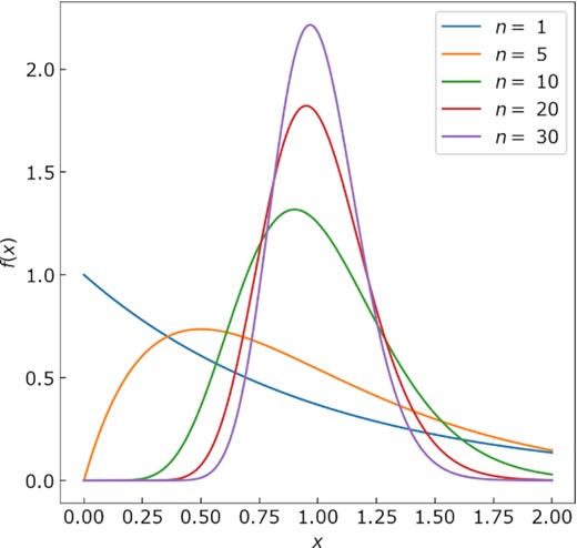
Plot of eq. (5), where |$\lambda = \frac{1}{n}$|, so that |$\bar{x}$| = 1.00 for an infinite sample. The peak probability (mode or maximum likelihood) occurs between |$\bar{x}$| = 0 for n = 1 and |$\bar{x}$| = 1 for an infinite sample.
Eqs (9) and (3) together are equivalent to eq. (7) of Ogata & Yamashina (1986), albeit derived by the maximum likelihood solution (near the mode in a finite sample) rather than the expectation value (near the mean). It confirms that we expect the most likely sample mean to start at zero in a sample of n = 1 and trend in a nonlinear fashion asymptotically to |$\bar{x} = \bar{x}_\infty$| from below.
Eq. (9) specifies the convergence of the most likely mean magnitude in a finite sample of events above mc as a function of the number of events n. However, the focus here is the dynamic range r = ω − mc where ω is the largest magnitude in a sample. We acknowledge the inherent connection between n and the dynamic range, where often (although not exclusively), small dynamic range will also have low n and account for dynamic range in the next section.
Accounting for a finite minimum in x
This formula can be used to correct for the systematic bias involved in the assumption that the mean magnitude |$\bar{m}$| is a good approximation for the expectation value 〈m〉 for an infinite sample in the derivation of Aki (1965). Important to note is that the mean magnitude will be influenced to some extent through magnitude binning (Marzocchi et al. 2020), however, when bins are 0.1 or less, the bias is generally negligible (as in the current case). The bias in the estimate λAki is then the difference between λAki and λ. Again, it is easy to show analytically from eq. (17) that λAki converges asymptotically to λ systematically from above, and hence b-values in data samples with small dynamic range are likely to be biased to high values.
3 METHODS AND DATA
The data used to test the hypotheses developed above include both synthetic and real earthquake magnitude data. For the synthetic data, we create 100 realizations on the real number line, of both ‘perfect’ GR and MGR catalogue data with the following parameters: n = 100 000, mmin = 0.5 and b-value = 1.0. For the MGR distribution, we take mθ = 5.0 because this is representative of small to medium magnitude earthquakes, compared to, for example, mθ ∼ 8.5 for the tectonic, global Harvard Centroid Moment Tensor (CMT) catalogue (Bell et al. 2013). The 95 per cent confidence intervals on the randomly sampled data are obtained from the scatter of the Monte Carlo simulations, and compared to the errors obtained for the real data using eqs (18) and (19) below which represent estimates of the irreducible random errors in |$\bar{m}$| and b, and hence the precision of the estimate. Our estimate of confidence intervals for the synthetic data may not be ideal in the case of small samples, where a chi-square distribution might be preferable, but we preferred to apply a consistent method, recognizing that the confidence intervals may not be ideally accurate in the smaller samples.
For the real earthquake catalogues, we have chosen two very different examples – The Geysers geothermal (induced) earthquake catalogue in California and the Southern California (tectonic) catalogue. Geffers et al. (2022) previously showed that The Geysers data are likely to exhibit an MGR preference at large dynamic ranges (and therefore large sample sizes), whereas in Southern California, GR is strongly preferred. This allows us also to examine the effect of the epistemic uncertainty caused by lack of knowledge of the underlying form of the distribution. In the following results section, we compare the outcomes for the synthetic GR and MGR data to those from The Geysers and Southern California data, and examine the extent to which eq. (17) describes the data. The Geysers catalogue contains over 60 000 events in the complete part of the catalogue, where the magnitude of completeness mc = 1.25 as estimated by the b-value stability method (Wiemer & Wyss 2000; Cao & Gao 2002). This method was also used to estimate mc for Southern California, given as 3.28. This leaves 9023 events remaining in the complete part of this catalogue. The largest observed magnitude in The Geysers catalogue is 5.01 and 7.30 for Southern California. This results in maximum observed dynamic ranges of 3.76 and 4.02, respectively.
To estimate the best fit free parameters in eqs (15) and (17) for the synthetic data, we used the nonlinear least-squares curve fit function scipy.optimize.curve_fit in Python. The curve_fit function then returns optimal values for the parameters. We find a secondary local mode that is an artefact of small samples containing fewer than three data points, described in more detail in the results section, so these outcomes are discarded before fitting the data.
For the case of the real catalogues, using the curve_fit function is problematic because it assumes that residuals are random, which can result in poor fits to the actual data. Therefore, we opted for a different approach when fitting eqs (15) and (17) to the real data. The parameters |$\bar{m}_\infty$| and λAki (equivalent of bAki) were estimated instead from the value of the data point at largest dynamic range. This assumes that convergence is reached within the observed catalogue data. Having fixed these values at asymptotic convergence, we vary dm to the optimal incremental magnitude bin size which will fit eqs (15) and (17) as closely as possible to the real catalogue data.
These error estimates represent the irreducible, random errors in our estimates of |$\bar{m}$| and b. We consider an estimate of the mode in |$\hat{b}$| to be accurate when the systematic error or bias |$\hat{b} - b \le$| 0.1, and to be precise when δb ≤ 0.1. In the case of the real data, the true values of |$\bar{m}$| and b are not known, so we cannot define an accuracy. The equivalent (rounded) criteria for the estimates of mean magnitude are a bias |$\hat{\bar{m}} - \bar{m}_\infty \le$| 0.05 and a precision |$\delta m \le \frac{0.1}{\ln (10)} \le$| 0.05. Strictly exact equivalence occurs when |$\delta m \le \frac{0.1}{\ln (10)}$| but pragmatically we choose the approximation |$\frac{0.1}{2}$| here in rounding to the nearest multiple of 0.05. In the case of the synthetic data, there are multiple catalogues, and the resulting data scatter provides a more complete range of uncertainties. In this case, the confidence intervals are estimated from the random data scatter. These reflect better the total uncertainty, including the epistemic uncertainty resulting from lack of complete knowledge in a single finite sample.
In the synthetic data, the true b-value is taken to be 1.0, consistent with many examples in the published literature where there is a good dynamic range of data (Frohlich & Davis 1993; Kagan 1999). However, in the real data, both the true distribution of the data and the true underlying b-value remains unknown, inevitably introducing a systematic uncertainty which we need to account for. Therefore, for the real data, we assume that convergence is reached within the data available here and that convergence to the asymptotic value of |$\bar{m}_\infty$| and b is established at least approximately at largest dynamic range for both |$\bar{m}$| and b. We acknowledge that this pragmatic assumption could lead to an unavoidable residual bias not accounted for in our analysis of the real data below. The estimated values of b and mθ in the real data are obtained using eqs (4) and (5) in Geffers et al. (2022), using the method of Kagan (2002) to define maximum log-likelihood functions for the distribution for a finite sample of n observations. The resulting best estimates β (equivalent of b) and Mθ (equivalent of mθ) are obtained for the real data and are shown in Table 1.
Threshold dynamic ranges for accuracy ra and precision rp at 95% confidence as a function of mc, m∞, and the assumed or estimated b-value and corner magnitude mθ. The bias or precision respectively are defined when they are equal to 0.05 units in |$\bar{m}$| and 0.1 units in b (Fig. 2). The accuracy cannot be estimated for the real data because the underlying values are not known.
| Figure | Data | |$r_a(\bar{m}$|) | |$r_p(\bar{m}$|) | ra(b) | rp(b) | mc | Estimated |$\bar{m}_\infty$| | Estimated b-value | Estimated mθ |
|---|---|---|---|---|---|---|---|---|---|
| 2(a) and (b) | Synthetic GR | 3.6 | 4.0 | 3.0 | 3.8 | 1.0 | 1.43 | 1.00 | 3.5 |
| 2(c) and (d) | Synthetic MGR | 1.7 | 2.6 | 1.7 | 2.0 | 1.0 | 1.42 | 1.00 | 3.5 |
| 3(a) and (b) | The Geysers | - | 2.0 | - | 2.2 | 1.25 | 1.66 | 1.02 | ∼ 4.6 |
| 3(c) and (d) | Southern California | - | 3.0 | - | 2.7 | 3.28 | 3.70 | 1.04 | ∼ 7.0 - 7.5 |
4 SYNTHETIC AND REAL CATALOGUE RESULTS
We now present the results of the hypothesis test on both synthetic and real earthquake catalogue examples, using the theory and methods described in the previous two sections. The figures in this section all follow the same visual representation—the catalogue data are shown as blue circles, where red circles indicate discarded data (n ≤ 3), orange circles indicate data with n > 50 and the solid black line represents the sampled mode from the remaining data. All of the discarded mean magnitude data with n = 1 in any sample plot on a straight line (shown in brown in the case of synthetic data in Fig. 2) and represent a hard edge to the range of possibilities—a clear artefact of such small samples. This logic extends to the choice of n ≤ 3 to avoid artefacts from a secondary local mode summarized in section 3. The area in light blue represents the 95 per cent confidence intervals of the outcomes determined by (a) the scatter in the results for the synthetic data or (b) the error estimates given in eqs (18) and (19) of |$\bar{m}$| and b for the single samples in the real data, also at 95 per cent confidence. Faint, horizontal lines indicate the optimal convergence values of |$\bar{m}$| and b returned from fitting eqs (15) and (17).
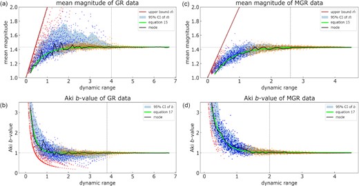
(a) and (c) Mean magnitude as a function of dynamic range for GR and MGR data, respectively. (b) and (d) b-Values as a function of dynamic range for GR and MGR data, respectively. The straight brown line in all plots indicates an upper bound to the mean magnitude in a sample of 1. The solid black line shows the mode for the plotted synthetic data (blue circles) and the bright green curve represents eq. (15) in (a) and (c) and eq. (17) in (b) and (d). The vertical dotted line represents the point at which both accuracy and precision are reached and the horizontal, dotted line represents the optimal values for convergence of |$\bar{m}$| or b obtained from the curve fit. Red circles indicate discarded data where a sample n ≤ 3. Orange circles indicate data where a sample n > 50.
In Figs 2(a) and (b), the data are randomly sampled from a GR distribution with b = 1. In Fig. 2(a), |$\bar{m}$| converges from below as a function of dynamic range and there is good agreement between the mode and that predicted by eq. (15) in bright green. For a dynamic range of ∼ 1.4 and up, the mode already lies within ± 0.05 units of |$\bar{m}_\infty$|. Fig. 2(b) shows the corresponding Aki b-values as a function of dynamic range. The best fit (eq. 17) converges extremely quickly to b = 1.0 ± 0.1, similar to the mode, before a dynamic range of 1.0 is even observed. This convergence is somewhat faster than in the case of the mean magnitude because of the approximation involved in rounding described above. In the case of data randomly sampled from an MGR distribution, the dynamic range observed in the synthetic data where both accuracy and precision are attained is considerably smaller than for the GR data, due to the effect of the ‘corner’ magnitude mθ and the associated roll-off in frequency for larger events. In Figs 2(c) and (d), the data are randomly sampled from an MGR distribution with b = 1 and a corner magnitude of mθ = 3.5. The best fit for |$\bar{m}$| and b is very close to the observed modes although this time, in the case of the b-value, a dynamic range of around 1.3 is required for convergence to b = 1.0 ± 0.1 again, convergence to the benchmark value is slightly faster than in the case of the mean magnitude (Fig. 2c) which requires a dynamic range of 1.6 to fall within ± 0.05 units of |$\bar{m}_\infty$|.
In the case of The Geysers data, the last datapoint in Fig. 3(a) is ignored in the fit, as appears to be an outlier, and hence may bias the fit to the other estimates. For both |$\bar{m}$| and b in the case of The Geysers (Figs 3a and b), the convergence of the best fits to eqs (15) and (17) respectively, are very close to the predicted mode (specifically the maximum likelihood value) of the single sample catalogues across all dynamic ranges. Notably, in the case of |$\bar{m}$|, the fit overestimates the modal |$\bar{m}$| between dynamic ranges of 1.5 and 3.5, most likely due to the variability of real data associated with catalogue heterogeneity. We estimate |$\bar{m}_\infty$| is ∼ 1.66 and the associated b-value at convergence is b ∼ 1.0. On the contrary, the best fits do a less good job in fitting to the Southern California data shown in Fig. 3(c) and (d). This is also likely due the larger variability in the real data. The best fit parameters obtained in Fig. 3 are for (a) b = 1.5, dm = 0.05, (b) b = 1.01, dm = 0.11, (c) b = 1.05, dm = 0.01 and (d) b = 1.03, dm = 0.012.
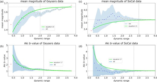
Presented as explained in the caption to Fig. 2. (a) and (c) Mean magnitude as a function of dynamic range for The Geysers and Southern California data, respectively. (b) and (d) b-Values as a function of dynamic range for The Geysers and Southern California data, respectively. Light blue shading represents the 95 per cent confidence intervals from eqs (18) and (19). The vertical dotted line represents the point at which precision is reached and the horizontal, dotted line represents the optimal values for convergence of |$\bar{m}$| or b.
Table 1 presents a summary of the threshold dynamic ranges required for accuracy and precision of |$\bar{m}$| and b for both the synthetic and real data sets, including their estimated values of convergence for |$\bar{m}$| and b. The increase in precision for both the synthetic (δbS) and real (δbR) with respect to r is shown in Table 2. In all cases, precision increases with respect to r. The synthetic data emulating the Southern California example converges more slowly than that for the real data, indicating that the total error may be underestimated by eq. (19), by a factor in the range 0.9–3.0. For the Geysers data, convergence in δbS and δbR is more similar to that expected from eq. (19), with a ratio near 1.0. Notably, the bias discussed here is mostly related to small r and n, and becomes less significant with increased r. While this may represent a minority of all studies of the earthquake frequency magnitude relation, these are over-represented in the case of volcanic and induced seismicity where the dynamic ranges are much smaller.
Convergence of the precision in the estimated b-value (δb) as a function of dynamic range for GR and MGR sampled data compared to Southern California and The Geysers data, respectively. For the synthetic data, δb is estimated from the scatter in outcomes at 95% confidence, denote δbS and for the real data from eq. (19), also representing 95% confidence, denoted δbR. The rows in bold state the ratio of |$\frac{\delta b_S}{\delta b_R}$|.
| Figure | Data | r = 1.0 | r = 2.0 | r = 3.0 | r = 4.0 |
|---|---|---|---|---|---|
| 2(a) and (b) | Synthetic GR | 1.0 | 0.65 | 0.4 | 0.06 |
| 3(b) and (d) | Southern California | 1.1 | 0.45 | 0.15 | 0.02 |
| Ratio |$\frac{\delta b_S}{\delta b_R}$| | 0.9 | 1.4 | 2.7 | 3.0 | |
| 2(c) and (d) | Synthetic MGR | 0.65 | 0.2 | 0.06 | – |
| 3(a) and (b) | The Geysers | 0.95 | 0.2 | 0.05 | – |
| Ratio |$\frac{\delta b_S}{\delta b_R}$| | 0.7 | 1.0 | 1.2 | - |
5 DISCUSSION
In our analytical theory, we have used a similar approach to that of Ogata & Yamashina (1986) who also used eqs (4) and (5) to derive eq. (9), as in this paper. However, there are differences. For example, we use a maximum likelihood solution for the mode of the distributions of mean magnitudes rather than the expectation value estimated from the mean value of a randomly selected set of mean magnitudes, but it is reassuring that the same result can be obtained from different methods. We then recast eq. (9) in terms of dynamic range, and examine how well this equation fits results from a finite size sample with a maximum observed magnitude ω. We also consider the assumption that the mean sampled magnitude is a good approximation for the expectation value, which in a finite sample is generally not the case. The maximum observed magnitude in the cases here are those that emerge from finite samples of either the real data or the generated synthetic data, that is we have not limited this correction a priori by setting a specific upper bound before the sampling.
The analysis of the synthetic data has shown that the convergence of the mode in the mean magnitude expected in a finite sample (eq. 15) in the case of an exponential FMD is in very good agreement with the observed value (Fig. 2). While the trends are broadly similar, this is not as clearly the case for real data. Nevertheless, the analysis of The Geysers data seem to follow this trend more closely than in the case of Southern California, where the picture is much more variable, leading to much larger uncertainties compared to The Geysers, most likely due to catalogue heterogeneity. Additionally, the real catalogues are already subject to larger uncertainties because the errors in both |$\bar{m}$| and b for a single sample are not representative of the overall uncertainty one might expect on repeating the experiment many times (Marzocchi & Jordan 2017,provide a detailed discussion on caveats associated with handling different sources of uncertainties).
In the case of the synthetic data, we know that b = 1.0. However, in the case of the real catalogue data, we do not know one ‘true’ value of b, even though Geffers et al. (2022) have previously suggested that of The Geysers catalogue is likely to have a b-value close to 1.0. This falls within the b-values estimated in prior literature, ranging from b ∼ 0.8 to 1.3 (Henderson et al. 1999; Convertito et al. 2012; Kwiatek et al. 2015; Leptokaropoulos et al. 2018). Similarly, b ∼ 1.0 for Southern California (Kamer & Hiemer 2015). These independent estimates are in agreement with the asymptotic b-values estimated in Table 1 of this study.
The improvement in accuracy of the estimated b-value in synthetic cases as a function of dynamic range (Table 1) can be attributed to the improvement in the estimated mean magnitude as sample sizes increase, captured in eq. (17) and in agreement with Ogata & Yamashina (1986) who state that the bias in b is ‘not small’ when n is small. This also concurs with the reduced bias in the b-value with respect to dynamic range as portrayed by fig. 6 in Marzocchi et al. (2020). Table 1 highlights the fact that one can obtain answers that are accurate but not precise, precise but not accurate, or accurate and precise, depending on dynamic range and the nature of the input catalogues. Table 2 suggests that the uncertainty expressed in eq. (19) may be an underestimate of the total variability in the results for the multiple realizations of the synthetic data for the same underlying distribution. Comparing the convergence of the b-value shown in Figs 2 and 3 as a function of dynamic range to previous studies (Marzocchi et al. 2020; Geffers et al. 2022), we show agreement that the bias reduces strongly if there are 3 orders of dynamic range available. In the case of synthetic GR data, we show that this decreases further with more dynamic range but it is unrealistic to expect such large dynamic ranges to be observed in any given real catalogue. The bias implied by the trend on the graphs for the real data is of a similar order of magnitude to that of the synthetics, but this will definitely be affected by binning forced by magnitude precision in the case of the real data. Hence, it looks as if this additional bias may be smaller or similar to, but not significantly larger than, that of the finite sampling, at least for small to intermediate dynamic ranges. At larger dynamic range, the real data does show a residual systematic bias that cannot be accounted for by the ideal theory alone.
The theory for the sampled synthetic data explicitly assumes events are independent and identically distributed (iid) in the case of a perfect, homogeneous catalogue of magnitudes with zero measuring uncertainty. However, in a real catalogue, the magnitude estimates are subject to uncertainty, and are measured indirectly from an evolving network with a finite number of stations with a finite sample of the radiation pattern, which in turn leads to much larger variability in the convergence trend and often a lack of convergence to a flat asymptote. It is worth noting that the catalogues used here have not been declustered, as most declustering techniques (Gardner & Knopoff 1974; Gerstenberger et al. 2020) do not preserve the uncorrelated magnitude distribution because they systematically remove smaller magnitude events.
There is some clear dynamic range dependent natural variability in the trends of the real data beyond that which can be explained by the theory in the case of the real catalogues, including at larger dynamic ranges (Fig. 3). Our interpretation is that this is most likely due to a mixture of catalogue inhomogeneity, magnitude uncertainties and binning (Bender 1983; Marzocchi et al. 2020) for the real data. These effects propagate into slower convergence to the asymptotic value for an infinite sample within the finite range observed. The ideal synthetic test data suffer from none of these complications. Further work is required to isolate the contributions to the trends in the dynamic range dependent variability shown on Fig. 3.
Finally, we note that Yaghmaei-Sabegh & Ostadi-Asl (2021) have independently examined the issue of convergence in the MLE of b-value of finite samples, focusing only on the sample size n. Here, our results demonstrate that it is equally important to consider the effect of dynamic range.
6 CONCLUSION
The mean magnitude of an earthquake catalogue converges to an asymptotic limit from below in random samples, consistent with a hypothesis derived analytically from the expected modal values in the sampled mean magnitude in such samples. In real data, the trend is broadly similar, but in detail substantially more variable. In this case, the true b-value is unknown, the catalogue magnitudes have a finite error, and the catalogue is likely to be heterogeneous, explaining many of the uncertainties involved in fitting eqs (15) and (17).
The dominant factor controlling the bias of high b-values is the convergence of the mean magnitude with respect to dynamic range, where the mode of the data matches the maximum likelihood expected in a random sample, when enough data and dynamic range are observed. In samples with a small dynamic range, the estimated mean magnitude is systematically and significantly underestimated, hence leading to an overestimate of the b-value as dynamic range reduces. While the bias is smaller than the scatter in the data, it is still likely to produce systematically high b-values on average from small catalogues with narrow dynamic range. Furthermore, we have shown that a stable estimate of |$\bar{m}$| is a prerequisite for obtaining a stable b-value estimate.
Overall, this novel analysis indicated that many published studies in the literature use dynamic ranges where we would expect significant bias in the b-value, resulting in a systematic error (underestimation) in the likelihood of large events in a larger sample, and hence an underestimation of the associated hazard obtained by extrapolation to larger event sizes, as may be the case when using eq. (19) on both GR or MGR data in the synthetic cases. This study highlights once again the importance of having enough data in any study involving power-law scaling of a physical source size, and hence an exponential distribution in a logarithmic magnitude parameter.
It is prudent to adopt a cautious interpretation of b-values and their importance and significance in seismic hazard analysis. There is no ‘one size fits all’ answer to how many events or what dynamic range is required in specific catalogues for an accurate or precise estimate of b. Nonetheless, the b-value estimates become more accurate and precise as the sample size and its dynamic range increases. These conclusions are not restricted to the applications in earthquake hazard, because a range of natural hazards exhibit power-law frequency–size distributions as described in the introduction, resulting in an exponential frequency–magnitude relation. Hence, the same issues of convergence, accuracy and precision in finite samples will apply and should be taken into account.
ACKNOWLEDGEMENTS
We would like to thank two anonymous reviewers and K. Bayliss for their constructive comments on our manuscript, helping to improve clarity. We would like to acknowledge the support for this work by the NERC E3 Doctoral Training Partnership grant NE/L002558/1. No conflicts of interest exist. For the purpose of open access, the author has applied a Creative Commons Attribution (CC BY) licence to any Author Accepted Manuscript version arising from this submission.
DATA AVAILABILITY
The Geysers catalogue was downloaded from the United States Geological Survey (USGS, https://earthquake.usgs.gov/earthquakes/search/ last accessed December 2020) and the Southern California data was accessed through the Southern California Earthquake Data Center (SCEDC, 2013, https://service.scedc.caltech.edu/eq-catalogs/date_mag_loc.php).
