


SUMMARY
Practical hybrid approaches for the simulation of broad-band ground motions often combine long-period and short-period waveforms synthesized by independent methods under different assumptions for different period ranges, which at times can lead to incompatible time histories and frequency properties. This study explores an approach that generates consistent broad-band waveforms using past observation records, under the assumption that long-period waveforms can be obtained from physics-based simulations. Specifically, acceleration envelopes and Fourier amplitude spectra are transformed from long-period to short-period using machine learning methods, and they are combined to produce a broad-band waveform. To effectively obtain the relationship of high-dimensional envelopes from limited amount of data, we (1) formulate the problem as the conversion of probability distributions, which enables the introduction of a metric known as the Wasserstein distance, and (2) embed pairs of long-period and short-period envelopes into a common latent space to improve the consistency of the entire waveform. An experimental application to a past earthquake demonstrates that the proposed method exhibits superior performance compared to existing methods as well as neural network approaches. In particular, the proposed method reproduces global properties in the time domain, which confirms the effectiveness of the embedding approach as well as the advantage of the Wasserstein distance as a measure of dissimilarity of the envelopes. This method serves as a novel machine learning approach that maintains consistency both in the time-domain and frequency-domain properties of waveforms.
1 INTRODUCTION
The estimation of broad-band (BB) ground motions resulting from future earthquakes is indispensable for hazard assessment and engineering design (a glossary of abbreviations can be found at the end of this manuscript). With the development of high-performance computing, physics-based numerical simulation (PBS) has become a leading tool for estimating ground motions (e.g. Graves 1996; Bao et al. 1998). It solves wave equations by modelling the earthquake rupture process, propagation of seismic waves, and site responses in detail. However, its accuracy is currently limited to long-period (LP) ranges (approximately 1 s and longer) because of limited knowledge of rupture processes and ground structures at small scales. Therefore, accurate estimation of short-period (SP) waves is an important research direction.
Stochastic methods have been developed to synthesize SP waves, considering that incoherent behaviours dominate in this range. These are often combined with PBS in LP to synthesize BB time-series of ground motions (e.g. Kamae et al. 1998; Hartzell et al. 1999; Graves & Pitarka 2010). These methods, referred to as hybrid methods, produce waves with statistical properties in the time and frequency domains. However, because stochastic calculations are performed independently of PBS, fault-rupture and wave-propagation processes are not directly modelled in the SP range; consequently, the ground-motion characteristics are sometimes inconsistent between the LP and SP ranges. Thus, it is necessary to synthesize SP waves that bear the characteristics of LP waves computed using PBS.
In recent years, several studies have used empirical relationships between LP and SP ground motions obtained from observation records, to overcome the above drawbacks of hybrid methods (Iwaki et al. 2016; Paolucci et al. 2018). In both methods, LP waves are computed by PBS, while SP waves are estimated based on the empirical relationship between LP and SP ground-motion characteristics. Paolucci et al. (2018) is a pioneering study that applied a machine learning (ML) method to ground-motion estimations. It places weight on the engineering characteristics of ground motion and constructs a neural network to estimate the spectral acceleration at SP from that at LP. The PBS LP waveforms are enriched by stochastic SP waveforms to match the estimated acceleration spectra. This approach achieved realistic patterns of peak ground acceleration correlated with PBS, but the resulting waveform does not necessarily reproduce the properties of travelling waveforms in the time domain.
In contrast, Iwaki et al. (2016) treated root-mean-square (RMS) acceleration envelope waves to reproduce the characteristics of ground motions in different frequency bands. The PBS LP waves can be transformed to the corresponding SP waves by multiplying with the ratio of the amplitudes of SP and LP envelopes, called the envelope ratio function (ERF). Iwaki et al. (2016) estimated the ratio by regression analysis of observation data from earthquakes that occurred in the region near a target earthquake location. This approach enables us to project the characteristics of PBS LP waves on SP waves in the time domain; however, envelopes are modelled by three parameters (scale, duration, and decay constant), and observation data are manually selected. This limits the representative power of waveforms and degrades objectivity.
In Japan, strong-motion observation networks such as the K-NET and KiK-net have been operated over the past 20 yr by the National Research Institute for Earth Science and Disaster Resilience (NIED; NIED 2019a), and ground-motion data have been systematically collected. Taking advantage of these big data, we propose an ML approach to estimate BB ground-motion waveforms (Fig. 1). The procedure mainly consists of the conversion of RMS envelopes and Fourier amplitude spectra from the LP to SP ranges using ML models. We construct a novel embedding-based ML model to convert envelopes as follows: pairs of LP and SP envelopes are embedded into a common latent space, and unknown SP envelopes are interpolated from neighbourhoods in the latent space. To effectively capture the entire shape of the envelopes, we reformulate the procedure as the conversion of probability distributions, which enables us to introduce an advanced dissimilarity measure, the Wasserstein distance. By estimating amplitude spectra using neural networks, time-series of BB ground motions are synthesized.
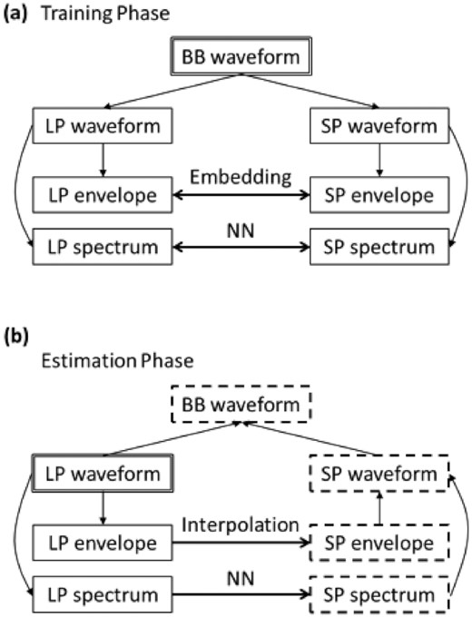
Flow chart of ground-motion estimation in this study. Double line frames represent input data, and dashed frames represent data obtained using ML methods. (a) Training phase. Observed BB acceleration waveforms are processed to LP/SP envelopes and amplitude spectra. ML models learn the relationship between LP and SP components of envelopes and spectra. (b) Estimation phase. For a given PBS LP acceleration waveform, envelope and spectrum are converted by trained ML models to corresponding SP envelope and spectra, respectively. They are synthesized to an SP waveform, which is combined with the input LP waveform to form a BB waveform. BB: broad-band; LP: long period; SP: short period; NN: neural network.
The Wasserstein distance originates from the optimal transport problem, which considers an optimal way to transform one probability distribution to another. It has profound geometric structures, and its research areas range from pure mathematics (Villani 2003, 2008) to practical applications such as economics, image processing and ML (Galichon 2016; Kolouri et al. 2017; Peyré & Cuturi 2019). In seismology, optimal transport has been introduced as a misfit measure in full waveform inversion (Engquist & Froese 2014; Métivier et al. 2016). These studies applied the Wasserstein distance to the oscillating time history of the waveforms. We apply it in a more straightforward way to the envelope of waveforms that have positive values.
In Section 2, we present a procedure for simulating BB ground motions based on the results of PBS. First, an embedding method for envelopes is described in detail; this method enables us to estimate the properties of waveforms with large dimensions, in the time domain. Then, a neural network approach to estimate the properties in the frequency domain and BB ground-motion synthesis are described. Section 3 describes the application of the proposed method to an M7 earthquake in Japan. Section 4 compares the results with those of existing methods, before concluding our work in Section 5.
2 PROPOSED METHOD
We propose a procedure for simulating BB ground motions of a target earthquake assuming that PBS provides a reliable result for LP (periods longer than 1 s). The properties of a target SP waveform in the time and frequency domains are separately estimated from the observed LP waveforms, using ML methods. They are then synthesized to an SP waveform, which is combined with the PBS LP waveform in the time domain to generate a BB waveform.
2.1 Waveform property in the time domain
We consider the RMS acceleration envelopes as representing the time-domain properties of the waveforms. Given an LP envelope, the challenge is to estimate the corresponding SP envelope. Observation records of past earthquakes are used as the training data. However, the number of records is still limited, especially for large earthquakes. Moreover, the relationship between LP and SP waves has a one-to-many correspondence due to the incoherency of seismic waves at small scales. These restrictions would prevent simple end-to-end deep neural networks from obtaining a precise relationship between the two. Difficulties arise because both LP and SP time-series belong to huge-dimensional spaces, while the amount of data is insufficient to ascertain the mapping from one time-series to the other. To effectively understand the correspondence, we construct a low-dimensional latent space that holds the information of both spaces. Once an LP envelope is obtained, the latent space representation can be used to estimate its SP counterpart.
Following the above consideration, we formulate an embedding-based approach to estimate SP envelopes (Fig. 2). Embedding is independently performed at individual sites, because the relationship between LP and SP envelopes should be significantly different among sites. First, pairs |$( {x_i^{{\rm{LP}}},x_i^{{\rm{SP}}}} )$| of observation (training) data of LP and SP envelopes are embedded as vectors |${{{\bf y}}_i}$| into a common latent space (subscripts i refer to earthquakes). Once the training data are embedded, for a PBS (target) LP envelope |$x_*^{{\rm{LP}}}$| (* indicates PBS), the corresponding unknown SP envelope |$x_*^{{\rm{SP}}}$| is interpolated based on the distribution around an embedded vector |${{{\bf y}}_*}$| in the latent space. It is critical to introduce a suitable distance measure on the envelope space, to perform an effective estimation. For this purpose, we (1) define a metric structure on the envelope space; (2) formulate an embedding method for observation data (both LP and SP waves are recorded) and PBS data (only LP waves are calculated); and (3) present an interpolation procedure using the neighbour relations in the latent space.
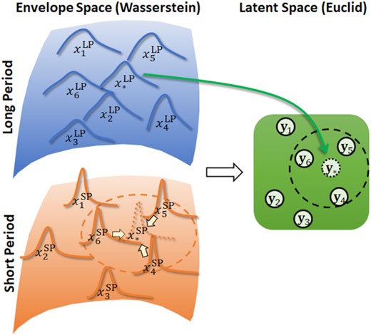
Schematic illustration of the proposed embedding method. Distributions of LP and SP envelopes are represented in high-dimensional spaces through definition of the proper metric (the Wasserstein distance). By embedding pairs of envelopes into low-dimensional Euclidean latent space using an extended version of t-SNE, a PBS LP envelope can be located in the latent space. The corresponding SP envelope is interpolated based on neighbour relations in the latent space. Subscripts refer to earthquakes, and * indicates PBS.
2.1.1 The Wasserstein distance
To extract the essential properties of time variations, we treat normalized envelopes in the analysis. Envelopes are obtained by taking the RMS of the original acceleration waveforms with 2 s time windows, and they are normalized so that time integration takes the value unity.
The definition of a metric structure in the envelope space is essential for the embedding. The |${L^2}$| distance is a natural choice for time-series data, but it has two critical shortcomings with regard to the current problem. First, it only measures the difference of amplitudes at each time step, and does not consider the difference in the time direction. For instance, the distance is constant irrespective of time separation as long as the two waves do not intersect. This shortcoming is apparent when we interpolate two waves; the linear interpolation of two waves are carried out independently at each time step, which leads to distortion in the resulting shape of the wave (Fig. 3a).
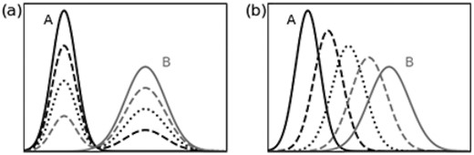
Interpolation between waves A and B using different metrics. (a) The |${L^2}$| distance linearly interpolates at each time independently, so the shape of waves (one peak) is distorted during the interpolation (two peaks). (b) The Wasserstein distance retains the shape and smoothly interpolates features such as the peak position, peak amplitude and wave width.
The other shortcoming of the |${L^2}$| distance is apparent from a comparison of waves generated by different earthquakes. There is no physical correspondence between the origin time of different signals, in contrast to error evaluations where both estimated and ground-truth waves represent an identical signal. Therefore, parallel-translated waves should be regarded as the same data; that is, the distance should be invariant under a time shift. A natural solution is to shift one of the waves to minimize the |${L^2}$| distance. However, this causes a problem; shifting of waves A and B to minimize the distances to wave C does not necessarily minimize the distance between waves A and B. In other words, pair-wise minimizations do not lead to global minimization, and there is no standard way to define a reference time for all data. This poses a problem particularly in the interpolation, because consistent time shifts cannot be set among neighbourhoods.
This is called the Wasserstein distance (|${W_2}$| distance). Here, minimization is performed over probability measures|$\ \gamma $| on |$X \times X$| with arguments |$( {x,y} )$| such that the marginal distributions with respect to x and y coincide with |${p_A}$| and |${p_B}$|, respectively (e.g. Santambrogio 2015). A prominent feature of the Wasserstein distance is that it inherits the geometry of the metric space X, referred to as the ground distance (Rubner et al. 2000). For instance, the Wasserstein distance between two disjoint distributions increases with the ground distance. This advantage is manifested in the interpolation; a whole shape is maintained by sliding a wave along the time direction (Fig. 3b).
2.1.2 Embedding
Embedding is performed mainly for dimensionality reduction or visualization of the original data. Principal component analysis (Pearson 1901) is a classical linear method that finds a projection of data with maximum variance. Various methods such as multidimensional scaling methods (Cox & Cox 1994), Isomap (Tenenbaum et al. 2000), and locally linear embedding (Roweis & Saul 2000) have been developed to deal with non-Euclidean distances and nonlinear manifold distributions. Because our goal is the interpolation of objects using neighbourhoods, only a local structure is significant. To this end, we refer to t-distributed stochastic neighbour embedding (t-SNE) proposed by van der Maaten & Hinton (2008), as the foundation of our embedding process.
We now develop an embedding method for LP and SP envelopes by extending t-SNE. A key point is that a pair of data in the two envelope spaces is projected onto a single point in a low-dimensional space. Therefore, embedded vectors |${{{\bf y}}_i}$| no longer merely compress the information of high-dimensional data as common dimensionality reductions, but code the relationship of the two envelope spaces as a latent variable that generates a correlated pair of data. Our task is to find a cost function that preserves both neighbour relationships while maintaining computational efficiency.
The optimal position of |${\cal Y}=\{\textbf{y}_i\}$| is determined by minimizing the cost function (8). Deviations from the LP and SP envelope spaces equally contribute to the cost function, and the resulting embedding would thus preserve both structures. In particular, neighbourhoods in the latent space are expected to be those in both the LP and SP envelope spaces.
The optimal position of |${{{\bf y}}_*}$| is determined by minimizing the cost function (11). Since the distribution |$\mathcal{Y}$| of training data holds the relationship of both LP and SP envelopes, this relationship should be reflected on |${{{\bf y}}_*}$|, although its position is determined from distances in the LP envelope space alone. This property is demonstrated in Section 4.1. In summary, the embedding is performed to minimize cost functions (eqs 8 and 11) that are designed to impose a large penalty when similar envelopes measured by the Wasserstein distance in the envelope space are placed to distant points measured by the Euclidean distance in the latent space.
2.1.3 Interpolation
Agueh & Carlier (2011) analysed this problem and introduced solutions called Wasserstein barycentres. This leads to acceptable interpolations that take the geometry of the base space into account (Cuturi & Peyré 2016). As shown in Fig. 3(b), shapes are preserved and features such as the peak position, peak amplitude, and wave width are neatly interpolated.
This has the same form as the Euclidean space (eq. 14); therefore, the solution is given by |$q_*^{{\rm{SP}}}\ ( x ) = \mathop \sum \limits_{k = 1}^K {w_k}q_k^{{\rm{SP}}}( x )\ $|. Its corresponding probability density yields the desired normalized envelope |$x_*^{{\rm{SP}}}$|.
2.2 Waveform property in the frequency domain
As the properties of ground motion in the frequency domain, we estimate the Fourier amplitude spectra in SP (1–50 Hz) from those in LP (0.01–1 Hz). The raw amplitude spectrum oscillates rapidly (Fig. 4a). To smoothen the spectrum, we take the RMS average over frequency windows whose ranges are set as |$< {10^{ - 2.0}}$| Hz, |${10^{ - 2.0}}$|–|${10^{ - 1.8}}$| Hz, |${10^{ - 1.8}}$|–|${10^{ - 1.6}}$| Hz, and every |${10^{0.1}}$| unit at higher frequencies up to |${10^{1.7}}$| Hz. As a result, we obtain a smooth spectrum in 19 and 17 bands in the LP and SP, respectively (Fig. 4b). The problem is now reduced to a simple regression problem that can be effectively modelled using a feed forward neural network. We set the LP spectra in the three components as the input variables (57 nodes), and the SP spectra in the three components as the output variables (51 nodes).
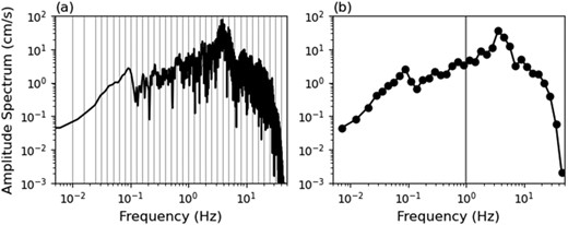
Smoothing of the Fourier amplitude spectrum. (a) The raw amplitude spectrum oscillates rapidly. Whole frequency range is divided into 36 bands (indicated by grey lines). (b) By taking the RMS average over spectra in each band, a smooth spectrum is obtained, which is used as input and output for the neural networks. A vertical grey line divides the LP and SP ranges.
The amplification of the SP spectra is strongly influenced by the underground structure beneath each observation site. The neural network should therefore obtain site-specific responses. However, the number of records at each site is severely limited. To balance these conflicts, we adopt the following two-step learning scheme (Girshick et al. 2014): a network is first trained using all records at all sites (first model); it is then retrained using records at a single site (final model). It is expected that the first step avoids overfitting, and the second step promotes adjustment to a site-specific relationship.
2.3 Broad-band ground-motion synthesis
3 APPLICATION TO AN EARTHQUAKE OFF IBARAKI PREFECTURE IN JAPAN
3.1 Ground-motion data
We apply the proposed method to a past earthquake. The target is an M7 earthquake that occurred offshore of Ibaraki Prefecture, Japan, at 01:45 JST (UCT + 9) on 2008 May 8 (Fig. 5). The ground-motion data are obtained from the strong-motion seismograph network, K-NET (NIED 2019a), during the period from June 1996 to September 2018. The seismographs record acceleration waveforms at 100 Hz sampling. The SP waveforms of the three components (north–south, east–west and up–down) are estimated at 18 stations in Ibaraki Prefecture, which provides 54 target data in total. To validate the method, LP waveforms are prepared by filtering the observation records instead of using PBS. Records whose peak acceleration values exceed 10 cm s−1 s−1, and whose squared amplitude accumulations of the first 100 and 120 s exceed 80 and 90 per cent of those of the whole records, respectively, are used. The latter condition is imposed to remove records of long duration or those failing to trigger a single event. This results in 2256 earthquakes (M2.2–8.1) and 12 833 records (200–1665 earthquakes at each site). Bandpass filters at 0.1–1 and 1–20 Hz are applied to generate LP and SP waves, respectively, and their RMS envelopes are calculated. To align the length of the data, the first 120 s from the beginning of the records are used by cutting signals or padding zeros, if necessary. Consequently, inputs and outputs are represented as 12 000-dimensional sequence data.
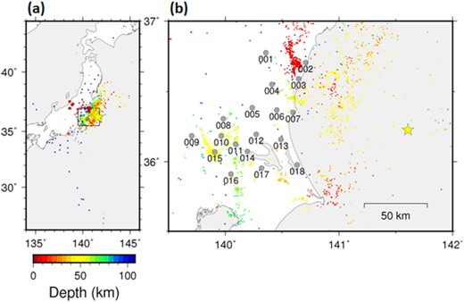
(a) Distribution of earthquakes used in the training of the neural network in Ibaraki Prefecture. A star represents the target earthquake, circles represent the 11 earthquakes used in training of the neural network (Table 1) and dots represent other training earthquakes. A rectangle demarcates the area shown in (b). (b) Distribution of observation sites. Grey circles represent observation sites with their labels, a star represents the target earthquake and dots represent training earthquakes. Colours of earthquakes represent the focal depth.
3.2 Model implementation
In embedding, we set a 3-D latent space and perplexity 50 as standard values (van der Maaten & Hinton 2008). The five nearest neighbourhoods are used in the interpolation.
In the estimation of Fourier amplitude spectra, we use a fully connected neural network consisting of two hidden layers each of which has {50, 50} nodes. The mean squared error in ln units is used as the loss function. The network is trained with the batch size of 100 for 10 000/1000 iterations in the first/second training step. The first/second training step is early stopped if the mean loss over the latest 1000/100 iterations does not reduce the mean loss over the previous 1000/100 iterations by 10 per cent. Overfitting, which is a common issue in neural networks, is critical in the current problem because the number of observation records is limited, especially those of large earthquakes. We add 1561 records collected at stations out of the Ibaraki Prefecture from 11 earthquakes with magnitudes greater than or equal 6.5 that occurred in the Kanto region (34|$^\circ $|–38|$^\circ $|N, 138|$^\circ $|–142|$^\circ $|E), to balance the number of records with different magnitudes (Table 1). These records are used only in the first training step.
List of earthquakes added to training data.
| Date | Latitude (deg) | Longitude (deg) | Depth (km) | Magnitude |
|---|---|---|---|---|
| 23 October 2004 | 138.867 | 37.291 | 13 | 6.8 |
| 23 October 2004 | 138.929 | 37.306 | 14 | 6.5 |
| 16 July 2007 | 138.608 | 37.557 | 17 | 6.8 |
| 11 August 2009 | 138.498 | 34.785 | 23 | 6.5 |
| 14 March 2010 | 141.817 | 37.723 | 40 | 6.7 |
| 11 March 2011 | 141.265 | 36.108 | 43 | 7.7 |
| 12 March 2011 | 138.597 | 36.985 | 8 | 6.7 |
| 11 April 2011 | 140.672 | 36.945 | 6 | 7.0 |
| 31 July 2011 | 141.22 | 36.902 | 57 | 6.5 |
| 19 August 2011 | 141.797 | 37.648 | 51 | 6.5 |
| 22 November 2016 | 141.603 | 37.353 | 25 | 7.4 |
Training data are often augmented by modifying input data in ML applications (e.g. Simard et al. 2003; Krizhevsky et al. 2012). For instance, image data are translated, rotated, or added small random noises for augmentation. As for seismic records, transformation of the horizontal axes (e.g. from ‘north’ and ‘east’ to ‘radial’ and ‘transverse’ components) yields realistic seismic records. Therefore, by rotating the horizontal axes and computing the amplitude spectrum in the new coordinates (both in the LP and SP ranges), the training data can be dramatically augmented in a physically realistic way. In this application, the horizontal coordinates are rotated by every 15° each, up to 180°, to increase the number of training data 12 folds. In total, 172 512 training data are used in the first step, and 2388–19 968 data at each site in the second step.
3.3 Results
The estimated normalized envelopes are compared with the observations in Fig. 6. Estimations reproduce the time history of the observed records, including the rise time, peak time and values, and decay rate. In particular, two peaks in the up–down component at site IBR001 are accurately estimated. This suggests the effectiveness of a non-parametric approach that does not assume a particular functional form for envelopes.
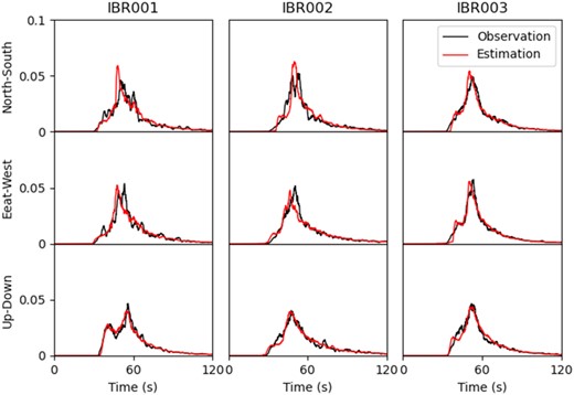
Comparison of observed (black) and estimated (red) SP (1–20 Hz) envelopes at selected sites.
As for the amplitude spectra, the RMS errors of the training and target data are 0.526 and 0.539, respectively, in the first step. The second step decreased the RMS errors of the training and target data to 0.395 and 0.405, respectively. This indicates the effectiveness of the fine-tuning approach. The difference of the RMS between the training and target data is small in both steps, which indicates the generalization performance of the network on unknown data. The comparison of outputs of the neural network for the target data with the ground truth is shown in Fig. 7. The first model estimates spectra that are too flat because it learns the average properties of all stations. In contrast, the final model shows sharp peaks consistent with the observed spectra. In particular, the peaks in the horizontal components approximately at 3 and 5 Hz at sites IBR001 and IBR002, respectively, are accurately reproduced. This suggests that site-specific responses are obtained in the second step.
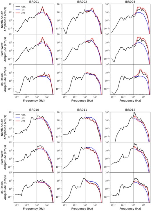
Comparison of observed (black lines) and estimated (colour lines) amplitude spectra at selected sites. Blue lines represent estimations of the first model, and red lines represent those of the final model. Vertical grey lines indicate separations between inputs (left, LP) and outputs (right, SP).
The neural network is expected to mainly model Green's function of wave propagations. When we focus on Green's function, which is independent of magnitude in linear responses, the network can learn the relationship between LP and SP spectra from ground-motion data caused by different size earthquakes. The network obtains dependence on source characteristics and propagation paths that have an influence on both LP and SP spectra. Local ground conditions have a significant influence on amplification of SP spectra, which makes it difficult to extract characteristics only from LP spectra. Therefore, the fine-tuning step at individual sites effectively works to obtain site-specific responses.
On the other hand, the peaks just above 1 Hz at sites IBR010 and IBR012 are poorly reproduced; the estimated spectra just above 1 Hz have similar values as the observed spectra just below 1 Hz, due to the continuity in most data. This indicates the difficulty in estimating sharp variations of spectra near but above the matching frequency. At site IBR003, the final model systematically estimates large amplitudes, although the first model does not. The SP spectra of moderate earthquakes are significantly amplified at this site, which would cause an overestimation of the SP spectrum of the target earthquake, whose LP spectrum is already large. This implies the difficulty of estimating accurate spectra of large earthquakes for which saturation of amplifications in SP could occur due to a nonlinear response of the surface soils.
The synthesized BB velocity waveforms are shown in Fig. 8. The velocities at site IBR003 are too high, reflecting the overestimation of amplitudes, whereas those at sites IBR010 and IBR012 are underestimated. In other stations, the synthetic time-series reproduce the observations well. There is no serious discrepancy in travel times between the LP and SP components.
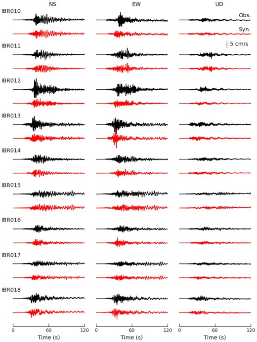
Comparison of observed (black) and synthesized (red) BB velocity waveforms.
4 DISCUSSION
4.1 Effects of embedding of acceleration envelopes
The main motivation for our study is the estimation of the realistic time history of ground motions. Here, we confirm that the embedding approach is successful in identifying appropriate neighbourhoods from past records. Although the training data are embedded using both LP and SP envelopes, the target data are embedded using only LP envelopes. The question then arises as to whether selecting neighbourhoods in the latent space leads to a better performance compared to simply selecting neighbourhoods in the LP envelope space. In Fig. 9, the distances between the training earthquakes and the target earthquake measured in different spaces are plotted at site IBR001. The relationship of distances measured in the LP and SP envelope spaces (Fig. 9a) shows a positive but blurred correlation. This results from the one-to-many nature of the correspondence. The relationship of distances measured in the latent and the SP envelope space shows a sharper correlation (Fig. 9b), with the correlation coefficient improving from 0.793 to 0.868. An embedded target vector |${{{\bf y}}_*}$| surely captures the neighbour relations of an unknown SP wave |$x_*^{{\rm{SP}}}$|.
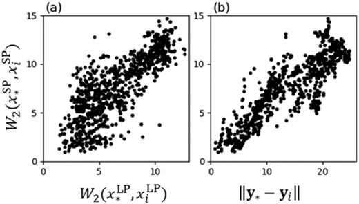
Distribution of distance between target and training data at site IBR001. Relationships of the distance in the SP envelope space and that in the (a) LP envelope space and (b) latent space are plotted. Each dot corresponds to one training earthquake i.
Focusing next on local correlations, which are more critical than global correlations for the estimation process, the distances between the SP envelopes of the target earthquake and SP envelopes of the five nearest neighbourhoods in the LP envelope and the latent spaces are computed. The average values of the distances over all target data are listed in Table 2. The results indicate that the SP envelopes of the neighbourhoods in the latent space are systematically closer to the correct envelopes than the neighbourhoods in the LP envelope space. This demonstrates that, when LP envelopes are obtained, the latent space works to reproduce the properties of the SP counterparts through the interpolation of neighbourhoods.
Average distance between SP envelopes of the target earthquake and those of five-nearest neighbourhoods in the LP envelope and latent spaces.
| Neighbourhood | LP envelope | Latent |
|---|---|---|
| 1 | 2.648 | 2.436 |
| 2 | 2.595 | 2.356 |
| 3 | 2.940 | 2.360 |
| 4 | 2.834 | 2.317 |
| 5 | 3.057 | 2.367 |
| Neighbourhood | LP envelope | Latent |
|---|---|---|
| 1 | 2.648 | 2.436 |
| 2 | 2.595 | 2.356 |
| 3 | 2.940 | 2.360 |
| 4 | 2.834 | 2.317 |
| 5 | 3.057 | 2.367 |
4.2 Extension to the neural network of amplitude spectra
This section discusses the extension to the neural network of amplitude spectra. Although the three components of LP spectra are used as the input variables, addition of earthquake parameters can be effective in reducing the loss function. We consider magnitude (M), focal depth (D) and epicentral distance (R), which can be obtained from the K-NET database. The results of RMS errors for all the combinations of M, D and R are listed in Table 3. The row ‘None’ corresponds to the proposed model in Section 3. The addition of M and D has little influence on RMS. This suggests that the shape of LP spectra contains the information of M and D, and the network obtains their dependence without explicit input of these variables. On the other hand, the addition of R significantly changes RMS, which suggests that SP spectra vary with source-to-site distance even if LP spectra are similar. The RMS reduces in the training data, but increases in the target data. This can be explained by the distribution of earthquakes; the training earthquakes are sparse around the target earthquake but dense in a northern area (Fig. 5). The network without R learns the regional difference of spectra, and successfully converts LP spectra of the target earthquake to SP spectra that bear the source and path characteristics around that event. In contrast, the network with R heavily relies on R, and outputs SP spectra that bear the characteristics in the data-rich northern region at similar distance. This implies that inclusion of R prevents the network from obtaining regional dependence, which could degrade the performance of earthquakes in a sparse area. In addition, the present network cannot extract directional dependence of SP spectra, such as basin effects. It would be therefore effective to construct a neural network that takes account of source locations, besides site specifications achieved by the fine-tuning procedure.
The root-mean-square errors of the neural networks with different input variables.
| Variables | First step | Second step | ||
|---|---|---|---|---|
| Training | Target | Training | Target | |
| None | 0.526 | 0.539 | 0.395 | 0.405 |
| M | 0.526 | 0.538 | 0.392 | 0.401 |
| D | 0.524 | 0.536 | 0.387 | 0.406 |
| M and D | 0.521 | 0.533 | 0.386 | 0.404 |
| R | 0.500 | 0.478 | 0.358 | 0.493 |
| M and R | 0.499 | 0.476 | 0.358 | 0.492 |
| D and R | 0.499 | 0.493 | 0.357 | 0.545 |
| M, D and R | 0.495 | 0.490 | 0.356 | 0.544 |
The transfer of the trained neural network to other regions, particularly regions where observational records are scarce, is of practical interest in applications. We consider Miyagi Prefecture as a target region, because three M7 class earthquakes of different types occurred (Table 4). Both Ibaraki and Miyagi Prefectures are located in a subduction zone of the Pacific plate. The ground-motion data are obtained during the period from January 2000 to December 2009 at 14 stations in Miyagi Prefecture where all the three target earthquakes were recorded (Fig. 10). The time period is limited to reduce the number of training data. This results in 541 earthquakes (M1.9–8.0) and 1831 records (30–329 earthquakes at each site). The following three neural networks are compared. First, a regional network is trained using data in Miyagi Prefecture, consisting of the first training step using all records at 14 sites in Miyagi Prefecture and the second training step using records at individual sites. Second, a host network is the same network as the first model in Ibaraki Prefecture. This model measures the applicability of the trained network to other regions. Finally, an adjusted network is constructed by training the host model using data in Miyagi Prefecture.
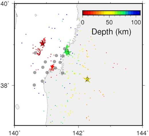
Distribution of earthquakes used in the training of the neural network in Miyagi Prefecture. Stars represent the target earthquakes, dots represent the training earthquakes and grey circles represent observation sites. Colours of earthquakes represent the focal depth.
Source parameters and root-mean-square errors of the neural network for the target earthquakes around Miyagi Prefecture.
| Parameter | Target 1 | Target 2 | Target 3 |
|---|---|---|---|
| Date | 26 May 2003 | 16 August 2005 | 14 June 2008 |
| Magnitude | 7.0 | 7.2 | 7.2 |
| Depth (km) | 71 | 42 | 8 |
| Tectonic type | Intraslab | Interplate | Crustal |
| Regional model | 0.934 | 0.803 | 0.897 |
| Host model | 0.909 | 0.801 | 0.864 |
| Adjusted model | 0.899 | 0.757 | 0.871 |
The RMS errors of the three networks are listed for each target earthquake in Table 4. The host network has a smaller RMS than the regional network. This suggests that training the network in another data-rich region under similar tectonics leads to a better performance than training the network in a data-poor target region. Moreover, RMS is larger than that in data-rich Ibaraki Prefecture (Table 3). These are common properties of data-driven approaches that do not impose physical constraints on the conversion. The adjusted network reduces RMS in most target earthquakes. Therefore, retraining of the host model to the target region is likely to improve the accuracy, even if available data are limited. The interplate event (Target 2) shows smaller RMS errors than crustal and intraslab events, because interplate events dominate in the subject regions. The specification of earthquake types would be essential in developing a neural network that is applicable to various tectonic regions.
4.3 Comparison with other methods
In this section, the proposed embedding method is compared with existing methods. We consider the following three approaches to BB ground-motion synthesis:
The proposed method (Embedding). This is the proposed method consisting of the embedding of normalized acceleration envelopes and the neural network of the Fourier amplitude spectra, as detailed in the previous sections. We refer to it as ‘Embedding’ in the following.
Stochastic Green's function method (SGFM). This is one of the conventional methods used to simulate the SP ground motion in hybrid methods. We follow the formulation of Dan & Sato (1998), which is used in the scenario earthquake shake maps of the National Seismic Hazard Map of Japan by the Headquarters for Earthquake Research Promotion (HERP). In the SGFM, the stochastic ground motion following the ω–2 source model (Boore 1983) of a small earthquake, or the stochastic Green's function (SGF), is synthesized on seismic bedrock (V∼3200 m/s, corresponding to the top of the upper crust) under the assumption of uniform propagation media and an attenuation model. Then, the SGF is summed over the fault of a large earthquake based on the self-similar scaling relations and the ω–2 source spectral model in a manner similar to the empirical Green's function method (EGFM) (Irikura 1986).
In this model, the short-period level A, or the acceleration source spectral amplitude at short periods, is approximately |$2.7 \times {10^{19}}$| Nm s−1 s−1, which is comparable to previous studies on the |${M_0}$|–A relations in the plate-boundary earthquakes around Japan (Satoh 2012; Nakano et al. 2015). The source parameters are listed in Table 5.
Source parameters for the stochastic Green's function method.
| Latitude (deg) | Longitude (deg) | Depth (km) | Seismic moment (Nm) | Effective stress (Pa) | Average slip (m) |
|---|---|---|---|---|---|
| 36.228 | 141.608 | 19 | 1.97E + 19 | 2.78E + 7 | 4.38 |
| Latitude (deg) | Longitude (deg) | Depth (km) | Seismic moment (Nm) | Effective stress (Pa) | Average slip (m) |
|---|---|---|---|---|---|
| 36.228 | 141.608 | 19 | 1.97E + 19 | 2.78E + 7 | 4.38 |
The horizontal and vertical components of the motion on the ground surface are computed using the multiple reflection theory for SH and SV waves, respectively, with vertical incidence, using a 1-D velocity structure from the seismic bedrock to the engineering bedrock extracted from the 3-D velocity structure model of the Kanto region used in the National Seismic Hazard Maps of Japan by HERP, and the surface soil model estimated from the logging data of K-NET at each site. The time-series of the ground-motion waveforms by the SGFM is generated by applying the statistical envelope model by Satoh et al. (1994), in which the envelope characteristics are described by a function of magnitude and distance. The SGFM waveforms are then superposed with the observed waveforms in the time domain to create time-series of BB ground motions at the crossover period (1 s) after applying a pair of low- and high-cut filters. This SGFM is adopted mainly for regional strong-motion prediction for shallow earthquakes, as in the National Seismic Hazard Map. The applicability of this method at larger distances has not be adequately validated; in fact, it has been reported that SGFM tends to underestimate SP ground motions at distances larger than 70 km (e.g. Iwaki et al. 2016).
Envelope ratio function (ERF). This is a leading method that considers the relationship between LP and SP waveforms in the time domain (Iwaki et al. 2016). First, 11 events that occurred near the source region of the target earthquake are manually selected. Then, the ERF is computed by averaging the amplitude ratio over the selected events. Finally, the SP envelopes are obtained by multiplying the ERF with the LP envelopes.
4.3.1 Time-domain property
In the evaluation of the performance of envelopes, we consider the following two models based on neural networks, besides the above two methods. These are designed only to estimate envelopes, and are not used to simulate BB ground motions.
Deep neural network (DNN). A simple way to apply neural networks is by constructing a feedforward neural network whose input and output are 12 000-dimensional vectors. We use a fully connected network consisting of four hidden layers each of which has {256, 128, 128, 256} nodes.
Sequence to sequence (seq2seq). Sutskever et al. (2014) constructed a neural network called sequence to sequence (seq2seq) that converts sequence data to sequence data by combining recurrent neural networks (Hochreiter & Schmidhuber 1997). This model has been widely used in language translation tasks. We apply this method by segmenting envelopes into several windows that contain the essential features of waveforms. We set the size of windows to 1000 samplings, i.e. 10 s.
We quantify the performance using two types of measures, namely, |${L^2}$| and |${W_2}$| losses. In Table 6, the mean and standard deviation of these losses over the target data are listed. Bold letters indicate the best models within one standard deviation. SGFM has the largest errors in both losses, resulting from independent calculations of LP and SP ground motions. It is important to generate SP motions that are consistent with the LP motions. In |${L^2}$| loss, which measures the local accuracy of waveforms at each time, seq2seq and Embedding show the best results, and ERF and DNN exhibit competitive performances. In |${W_2}$| loss, which measures the consistency of the overall shapes of envelopes, Embedding achieves the best result among the compared methods. The neural-network-based methods (DNN and seq2seq) degrade the performance compared with those in |${L^2}$| loss; seq2seq is comparable with ERF, and DNN is significantly worse than ERF. This implies that even if neural networks can simulate local behaviours, the global consistency of waveforms is not guaranteed, thus indicating the importance of considering the physical nature of waveforms. It is noteworthy that the embedding method achieves good results with respect to both criteria, even though only the Wasserstein distance is used in the embedding and interpolation processes.
Estimation errors of envelopes in |${L^2}$| and |${W_2}$| losses.
| Method | |${L^2}$| loss | |${W_2}$| loss |
|---|---|---|
| SGFM | 0.142 |$\pm $| 0.038 | 14.31 |$\pm $| 1.71 |
| ERF | 0.072 |$\pm $| 0.020 | 5.63 |$\pm $| 2.05 |
| DNN | 0.080 |$\pm $| 0.023 | 9.05 |$\pm $| 3.84 |
| seq2seq | 0.046 |$\pm $|0.012 | 4.36 |$\pm $| 2.54 |
| Embedding | 0.043 |$\pm $|0.018 | 1.92 |$\pm $|1.20 |
The estimated SP envelopes at site IBR001 are compared with the observations in Fig. 11. SGFM produces identical ground motions (hence envelopes and spectra) in the two horizontal components owing to the model assumption. SGFM envelopes have later travel time and shorter duration than observed envelopes, which leads to large misfits (Table 6). The other models show the correct travel time. ERF exhibits a sharp peak in the north–south component, which is possibly due to the influence of a spike in the LP envelope; the selected earthquakes are so few that estimations are vulnerable to the influence of outliers, although appropriate events are manually selected. DNN outputs almost identical waves for all components, suggesting overfitting to a typical pattern of the training data. This is because DNN tries to transform high-dimensional data without considering the neighbour relationships in the time axis, and it fails to extract various input–output patterns from the limited training data. Seq2seq reproduces the observation records more accurately. Compared with DNN, it extracts features of each window and transforms a sequence of features to another, which enables the network to learn relationships from the limited data. However, seq2seq shows artificial high-frequency oscillating behaviours. Embedding synthesizes smooth, realistic envelopes that simulate the global features of the observation records. This demonstrates the effectiveness of Wasserstein interpolation for high-dimensional but moderate-volume training data.
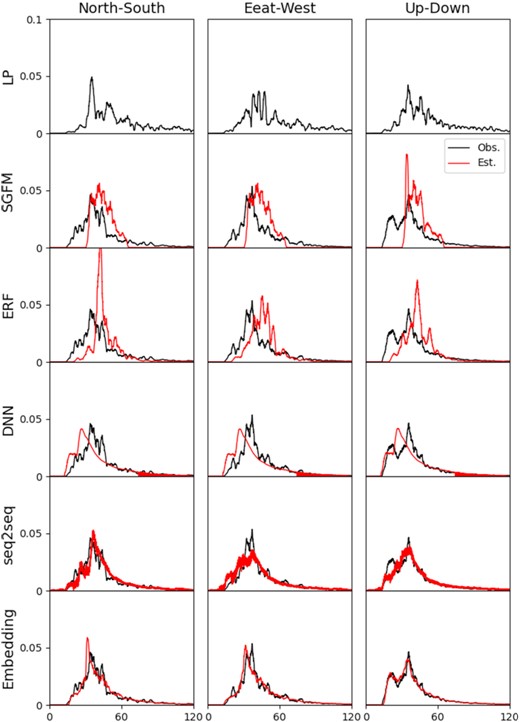
Comparison of estimated SP envelopes at site IBR001. Black and red lines represent observations and estimations of each method, respectively. Top panels show observed LP envelopes.
4.3.2 Frequency-domain property
The Fourier amplitude spectra of the BB acceleration waveforms are shown in Fig. 12. SGFM produces small amplitudes, as it tends to underestimate ground motions at distant area (the epicentral distances are larger than 70 km, as shown in Fig. 5), as stated earlier. In particular, the up-down components are small; the vertical motions are estimated using empirical horizontal/vertical ratios that have not been fully validated (Fujiwara et al. 2012). The large discrepancy results from a difficulty in modelling the source and propagation processes. On the other hand, the empirical approaches (ERF and Embedding) do not show underestimations. ERF models high-frequency components up to 16 Hz and shows reasonable amplitudes in this frequency range; it considers the frequency dependency of ground-motion amplitudes due to earthquake source spectra, as well as its site amplification characteristics. Embedding also shows good agreement with observations over a wide range of periods, and fits not only the overall intensity but also the change of amplitudes with frequency. A neural network is effective for taking account of ground conditions at each site.
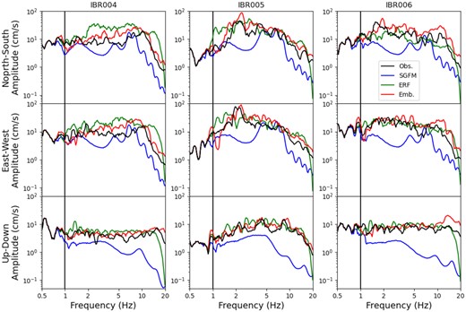
Comparison of Fourier amplitude spectra at selected sites.
We calculate the model bias for the Fourier amplitude spectra in SP, which is given by the natural logarithm of the observed over synthesized spectra at each frequency (e.g. Hartzell et al. 1999). Fig. 13 shows the mean and standard deviation of the model bias. SGFM has a positive bias (1 or larger, corresponding to an underestimation by one-third) and large uncertainty. ERF and Embedding have smaller biases than SGFM. ERF has little bias owing to the incorporation of source properties of earthquakes, but has large uncertainty owing to the small number of events available for fitting. Embedding has a small uncertainty over the entire frequency range, which implies that this method successfully fits the frequency dependence. The bias is mostly within one standard deviation, but is positive at 1–2 Hz. This is caused by the underestimation of the peaks around the matching frequency at several sites, as discussed in Section 3.3.
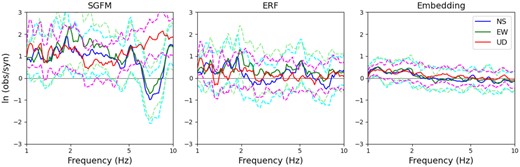
Model bias for Fourier amplitude spectra in SP. Solid and dashed lines represent the average residual and one standard deviation, respectively.
The goodness of fit of these methods with respect to frequency is measured by C9 (Anderson 2004) that quantifies the similarity of the Fourier spectra at specified frequency bands. A score of 10 indicates a perfect match, and scores of 0–4, 4–6, 6–8 and 8–10 are classified as poor, fair, good and excellent, respectively. Table 7 lists the scores in the three compared methods at four frequency bands. Although all methods have good scores at 1–2 Hz, this is because the BB waveforms are synthesized using observational records below 1 Hz. SGFM has a poor score at 2–4 Hz, and degrades the performance with frequency. This reflects a steep decay of amplitudes in high frequency (Fig. 12). ERF has lower but fair scores at higher frequencies. Embedding maintains good scores at all frequency bands, which indicates stability of the proposed method over a wide range of frequency.
Scores of the goodness-of-fit measure C9 (Anderson 2004).
| Frequency band (Hz) | SGFM | ERF | Embedding |
|---|---|---|---|
| 1–2 | 6.325 | 6.724 | 7.263 |
| 2–4 | 3.757 | 4.673 | 6.865 |
| 4–8 | 2.900 | 5.829 | 7.470 |
| 8–16 | 1.810 | 4.587 | 7.512 |
| Frequency band (Hz) | SGFM | ERF | Embedding |
|---|---|---|---|
| 1–2 | 6.325 | 6.724 | 7.263 |
| 2–4 | 3.757 | 4.673 | 6.865 |
| 4–8 | 2.900 | 5.829 | 7.470 |
| 8–16 | 1.810 | 4.587 | 7.512 |
4.3.3 Acceleration waveforms
The synthesized BB acceleration waveforms are compared in Fig. 14. The amplitudes of the SGFM waveforms are smaller than the observed waveforms, especially at site IBR003, where the ground amplification is high in SP. SGFM waveforms have arrival time and duration different from the observed waveforms at several stations. In addition, envelope shapes commonly have a simple form with a sharp rize and a heavy tail (Jennings et al. 1968). Although the shape of envelopes of the SP waveforms is represented by a formulation that reflects the statistical characteristics given the magnitude and hypocentral distances, they are not necessarily consistent with those of the LP waveforms. On the other hand, ERF and Embedding transform LP envelopes to SP envelopes, and thus arrival time and duration are almost consistent with the observations. Embedding reproduces time-domain properties such as moderate amplitudes before peak motions and the difference between horizontal and vertical components more correct than ERF, although the overestimation of amplitude spectra (Fig. 8) causes greater ground motions at site IBR003.


Comparison of BB acceleration waveforms at selected sites.
The model bias and RMS error for peak ground acceleration (PGA) and peak time are listed in Table 8. SGFM shows the largest RMS and a large positive bias in PGA, which indicates the underestimation of ground motions. Embedding shows a slightly smaller RMS than ERF; the value 0.428 corresponds to a factor of 1.5. Embedding shows a smaller RMS than ERF in peak time. This indicates the stability of an embedding-based ML approach compared to a manual-based empirical approach in the estimation of the time-domain properties. Although ERF and Embedding show the opposite bias in peak time, these values are sufficiently smaller than the RMS values.
Model bias and RMS for peak ground acceleration (PGA) and peak time.
| Method | ln (PGA cm s−1 s−1) | Peak time (s) | ||
|---|---|---|---|---|
| Bias | RMS | Bias | RMS | |
| SGFM | 0.771 | 0.910 | −4.58 | 8.63 |
| ERF | −0.247 | 0.496 | −1.19 | 8.65 |
| Embedding | −0.076 | 0.428 | 1.67 | 4.94 |
| Method | ln (PGA cm s−1 s−1) | Peak time (s) | ||
|---|---|---|---|---|
| Bias | RMS | Bias | RMS | |
| SGFM | 0.771 | 0.910 | −4.58 | 8.63 |
| ERF | −0.247 | 0.496 | −1.19 | 8.65 |
| Embedding | −0.076 | 0.428 | 1.67 | 4.94 |
Finally, the model bias for the synthesized time-series using 5 per cent damped acceleration response spectra in the SP are plotted in Fig. 15. The trend is similar to that for the Fourier spectra shown in Fig. 13 (note that the horizontal axis is frequency in Fig. 13 but period in Fig. 15). ERF and Embedding show small biases, and Embedding shows smaller uncertainty than ERF. Responses are systematically underestimated by SGFM, especially at shorter periods. In the SGFM, SP ground-motion waveforms are computed under several assumptions, that is, source model for SP wave radiation, wave propagation model from fault to site, and near-surface site amplification models, which result in the accumulation of modelling errors. In contrast, these assumptions are not required in the proposed embedding method because information on the 3-D wave propagation model is contained in the LP ground motion, and the amplification and envelope characteristics are obtained from the latent space for each site. Surface ground motions are directly obtained because most observation records are collected at the ground surface. Therefore, the results from the proposed method are expected to be more consistent with the observed waveform characteristics at each site.
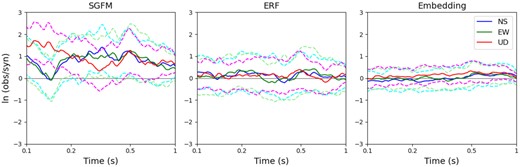
Model bias for 5 per cent damped acceleration response spectra in SP. Solid and dashed lines represent the average residual and one standard deviation, respectively.
5 CONCLUSIONS
We have presented a BB ground-motion synthesis that generates SP waveforms consistent with LP waveforms. Our main contribution is modelling of the time-domain as well as the frequency-domain properties using ML methods. We employed an embedding-based approach to effectively learn the relationship between high-dimensional LP and SP acceleration envelopes without imposing a particular form on them. Critical features of this method are (1) introducing the Wasserstein distance on the space of normalized envelopes to capture the global properties of waveforms and (2) simultaneously embedding LP and SP envelopes into a common latent space to obtain the relationship from a limited amount of data. An application of the proposed method to a past M7 earthquake demonstrated that it considerably improved consistency in the reproduction of the entire waveform (|${W_2}$| loss), while maintaining accuracy in a local measure (|${L^2}$| loss).
The BB waveforms were synthesized by estimating the Fourier amplitude spectra using neural networks. The two step training effectively worked to reduce fitting errors. The estimated spectra reproduced frequency-dependent site responses, although overestimation or underestimation occurred at several sites. Transfer of the trained neural network to another region exhibited good performance, and retraining of the network using few records at that region is likely to improve the performance. The experiments on additional input variables and predictions of different target earthquakes suggested that it is critical to incorporate source and path properties in maintaining high prediction accuracy for earthquakes occurring at different locations and tectonics. In the future, this study can be directed towards the development of such networks.
The proposed embedding method was able to extract the features of envelopes, and find neighbourhoods appropriate for constructing envelopes of target earthquakes. However, if the target is a large earthquake of the kind that has occurred rarely in the past, the interpolation process would not show good results, as with general ML methods that require big data. It would be especially difficult to estimate long-duration and multiple-rupture processes from past records. In general, the ground motions of large earthquakes are modelled by superposing ground motions of smaller element earthquakes. Formulating ML models with such an additive property would be effective for predicting the strong ground motions of unprecedented large earthquakes.
6 LIST OF ABBREVIATIONS
BB: broad-band, DNN: deep neural network, EGFM: empirical Green's function method, ERF: envelope ratio function, HERP: Headquarters for Earthquake Research Promotion, JMA: Japan Meteorological Agency, KL: Kullback-Leibler, LP: long period, ML: machine learning, NIED: National Research Institute for Earth Science and Disaster Resilience, PBS: physics-based numerical simulation, PGA: peak ground acceleration, RMS: root-mean-square, seq2seq: sequence to sequence, SGFM: stochastic Green's function method, SMGA: strong-motion generation area, SP: short period, t-SNE: t-distributed stochastic neighbour embedding.
ACKNOWLEDGEMENTS
Constructive comments provided by L. Alexander, K. Withers and an anonymous reviewer helped improve this paper. This study was supported by the Grant-in-Aid for Scientific Research (A) (Kakenhi No. 20H00292) from the Ministry of Education, Culture, Sports, Science and Technology (MEXT).
DATA AVAILABILITY
K-NET strong-motion data are available via the NIED website (https://www.kyoshin.bosai.go.jp). We used hypocentre catalogue by JMA (https://www.data.jma.go.jp/svd/eqev/data/bulletin/index.html). The 3-D velocity structure model of Kanto region by HERP can be obtained from J-SHIS website by NIED (http://www.j-shis.bosai.go.jp/labs/dstrctmap/).
