


SUMMARY
We analysed 478 three-component strong ground motion time-series from 65 events in the moment magnitude (Mw) 3–6.5 range recorded at 111 stations at distances up to 150 km from 1997 to 2019 in the Alborz region. Non-parametric spectral functions for seismological source, path and site-effects were derived from Fourier amplitude spectra of observed acceleration time-histories using the generalized inversion technique (GIT) for the Alborz region of Iran. To characterize the spectral models in terms of the anelastic attenuation (Q), geometrical spreading, magnitude and stress parameter (Δσ), we fitted non-parametric attenuation and source functions (resulted from inversion) with the standard parametric models. The frequency-dependent non-parametric attenuation function shows a rapid decay at close distances (<60 km) and decreases monotonically at larger distances. The frequency-independent geometrical spreading follows a bilinear hinged model with a crossover distance at 70 km. For hypocentral distances Rhypo < 70 km, the geometrical spreading is |${R^{ - 1.01}}$|, and for Rhypo > 70 km it is |${R^{ - 1.37}}$|. The corresponding quality factor is |$Q\ ( f ) = \ 146{f^{0.91}}$|. The non-parametric source spectra were found in a good agreement with Brune's ω-squared model. The stress-parameter (Δσ) values were found to exhibit large variability from 0.36 to 86.7 MPa with no significant magnitude-dependence. The average Δσ was found to be 8.6 MPa. The mean value of the estimated near-surface attenuation (κ0) from high-frequency part of non-parametric source function is 0.032 s (±0.01 s). In general, there is a good agreement between subsoil resonance frequencies and amplification levels estimated from GIT and HVSR (horizontal to vertical spectral ratio). The results of this study provide updated values of seismological source, attenuation and site properties in the Alborz region of northern Iran, which are expected to improve regional seismic hazard analysis studies in the region.
INTRODUCTION
The Alborz mountain range, that forms a part of northern margin of the Alpine–Himalayan collision zone in western Asia, is an active fold-and-thrust belt of approximately 100 km wide and 600 km long in the north of Iran, along the southern margin of the Caspian Sea. Alborz is bounded by Talesh Mountains in the east, Kopeh Dagh-Binalud Mountains in the west and grades to the Central Iran in the south (Mirzaei et al. 1998). The Alborz region is one of the most seismically active regions of Iran and it has been rocked by some of the devastating earthquakes in historical and instrumental time period namely, the Qumis earthquake of 22 December 1856 with surface wave magnitude Ms 7.9 (Ambraseys & Melville 1982) in eastern Alborz, and the Rubdar-Manjil earthquake of 20 June 1990 with moment magnitude Mw 7.3 (Berberian & Walker 2010) in western Alborz. In the recent past, the occurrence of several major earthquakes such as, 1997 Mw 6.5 Garmkhan, 2002 Mw 6.4 Changureh-Avaj, 2004 Mw 6.2 Baladeh (Kojour) earthquakes confirm the high seismicity in the Alborz belt of northern Iran. A pair of earthquakes on 11 August 2012 with Mw 6.4 and 6.2 shook the Varzaghan–Ahar region in northwest Iran. These two damaging earthquakes occurred in a region where there was no major mapped fault or any well-documented historical seismicity (Ghods et al. 2015). The foci of most earthquakes in Alborz are concentrated in the crust at depths less than 30 km. In terms of damage and loss of lives, the Rudbar earthquake is one of the largest, and deadliest, earthquakes in Iran. It affected both urban and rural regions, killed 13 000–40 000 people, and made a further 500 000 homeless (Berberian & Walker 2010). The Mw 6.4 Changureh-Avaj earthquake that occurred in northwest Iran (Qazvin province) killed 261 people and caused 1300 people injured and resulted in widespread damage, in spite of the low population density in this region. Similarly, the Mw 6.2 Baladeh earthquake of 28 May 2004 occurred near Baladeh (70 km north of Tehran) in the Alborz Mountains of northern Iran. Despite the moderate size of this earthquake, it was very significant. It was the first earthquake in the instrumental time periods to occur near Tehran (the capital city of Iran) that caused strong shaking within the city and the first large event to occur in the central Alborz Mountains since the Ms 6.8 28 July 1957 earthquake (Tatar et al. 2007). Evidently, the high seismic activity in this region poses significant seismic threat to Tehran with a population of around 13 million in the city and 23 million in the larger metropolitan area of greater Tehran along with some other major cities situated in this region. Thus, such high seismic activity demands better understanding of seismic hazard in the region thereby better potential risk estimation and disaster preparedness.
Estimation of potential ground motion is an essential element of any seismic hazard study (Cornell 1968; Reiter 1990). In engineering applications this is typically achieved by using, (1) empirically derived ground motion prediction equations (GMPEs) and (2) stochastic simulation method (Boore 1983, 2003). GMPEs are usually calibrated using recordings from past earthquakes and reliability of these empirical equations strongly depends on the quality and the quantity of the utilized database. For this reason, well-constrained GMPEs are often available only for well-monitored active regions such as California, Japan, southern Europe and the Mediterranean. The major issue with regional GMPEs derived in the recent past is the paucity of recorded data in the magnitude and distance range of engineering interest. The Iranian data set is sparse in the near distance range for earthquakes with M > 6.5 (Zolfaghari & Darzi 2019; Farajpour et al. 2019). GMPEs developed for Alborz region (e.g. Soghrat & Ziyaeifar 2016) suffer from lack of near-source data for large-magnitude earthquakes.
The stochastic simulation technique (Boore 1983, 2003) provides an efficient and reliable tool for generating synthetic ground motions of engineering interest. The stochastically simulated ground motions can be used either to develop GMPEs directly or to augment the existing recorded database (e.g. Atkinson & Boore 1995, 2006; Toro et al. 1997; Atkinson & Silva 2000; Raghu-Kanth & Iyenger 2007; Rietbrock et al. 2013). The seismological model used in the stochastic simulation is simple yet powerful enough to capture the essential scaling of ground motion with magnitude and distance. Typically, the stochastic (amplitude) model is characterized in terms of magnitude and stress-parameter (|$\Delta \sigma $|) as being the source parameters; the geometrical spreading and anelastic attenuation (Q) of seismic wave describe the path effects. The site effects are modelled in terms of crustal amplification (Boore & Joyner 1997; Joyner & Boore 1981; Boore 2003) and site-related attenuation parameter (|${\kappa _0}$|). Thus, a prior estimate of stochastic model parameters such as seismic moment |$({M_0})$|, |$\Delta \sigma $|, geometrical spreading, attenuation parameters Q and |${\kappa _0}$| is crucial for forward modelling of ground motions. Estimation of stochastic model parameters essentially involves separation of the source, path and site parameters from Fourier spectra of empirical recordings (Edwards et al. 2008; Drouet et al. 2010; Oth et al. 2011; Poggi et al. 2011; Edwards & Fäh 2013; Rietbrock et al. 2013; Pacor et al. 2016; Bora et al. 2017). Usually, two approaches namely parametric and non-parametric inversion schemes are adopted for estimating the stochastic model parameters from the recorded waveforms. The prominent studies that follow the parametric inversion scheme are Edwards et al. (2008), Drouet et al. (2010), Poggi et al. (2011), Edwards & Fäh (2013), Bora et al. (2015, 2017), while non-parametric inversion studies involve Parolai et al. (2000), Bindi et al. (2006), Oth et al. (2008), Bindi et al. (2009), Drouet et al. (2011) and Pacor et al. (2016). Initially, Castro et al. (1990) used generalized inversion technique (GIT) to find source spectra, S-wave quality factor and site response using records of nine moderate earthquakes (4 < Mw < 7) in a Guerrero, Mexico, subduction environment.
In the north of Iran, a limited number of studies have been carried out to investigate region-specific seismic source, path and site effects for the major seismotectonic provinces in recent years (e.g. Motazedian 2006; Zafarani et al. 2012; Ahmadzadeh et al. 2019). Motazedian (2006) used 259 three-component strong-motion accelerograms recorded within northern Iran from 22 events with Mw range 4.9–7.4 to examine the propagation characteristics of shear waves, including geometric spreading, Q, and κ0, and the local site amplification using horizontal-to-vertical spectral ratio (HVSR) method. Stochastic point-source and finite-source ground motion simulations were used to estimate the average stress parameter. Zafarani et al. (2012) used the generalized inversion of the S-wave amplitude spectra to estimate simultaneously source parameters, site response and S-wave attenuation (Qs). They considered 228 records from 29 earthquakes that were recorded at 81 strong-motion stations, with magnitudes (mb, Ms and Mw) in the range from 4 to 7.4, at focal depths from 5 to 32 km, and hypocentral distances ranging from 10 to 185 km. Ahmadzadeh et al. (2019) analysed 1117 seismograms from 312 crustal earthquakes recorded at the Iranian National Broadband Seismic Network in the Alborz region between 2005 and 2017 with ML 3–5.6 in the frequency range 0.3–20 Hz. They used S-wave spectral amplitudes and applied non-parametric GIT method to determine source parameters, path attenuation and site amplification functions.
In this paper, we estimated earthquake ground motion parameters by using an updated strong-motion database of recordings in the Alborz region of northern Iran. We used a non-parametric inversion technique to determine source, path and site effects. Estimation of source parameters involves determining M0 and |$\Delta \sigma $| for all the selected events. We estimated the geometrical spreading model and anelastic attenuation factor for the Alborz region. Furthermore, we presented empirical site amplification factors for some of the selected stations in the study region. All the seismological parameters estimated in this study are constrained by the (broadband) Fourier amplitude spectra (FAS) of the strong-motion accelerograms recorded in the study region. In addition to the use in simulation of ground motion, the seismological parameters in this study are expected to facilitate better understanding of source properties of earthquakes such as variations of |$\Delta \sigma $| in the Alborz region. Moreover, the derived anelastic attenuation function can provide additional insights regarding the path properties in the region. The estimated site amplification functions will be useful for applications such as site classifications and can play an important role for determining site-specific seismic hazard.
DATA SET SPECIFICATIONS
For this study, we used 478 three-component strong ground motion records from 65 events from 1997 to 2019 and 111 stations (Fig. 1) that were recorded by the Building and Housing Research Center (BHRC) of Iran (http://www.bhrc.ac.ir/). BHRC uses three kinds of instruments (SMA-1 analogue, SSA-2 digital and Guralp CMG-5TD digital) for recording strong ground motions. The sampling rate for majority of the instruments was 200 Hz while some of the instruments had sampling rate of 100 Hz. The selected data set consists of recordings from earthquakes in the magnitude range Mw 3–6.5 at distances up to 150 km (Table 1). The magnitude–distance distribution of the selected data set is depicted in Fig. 2(a). We only used crustal events with hypocentral depth up to 40 km. The magnitude–depth distribution of events is shown in Fig. 2(b). Out of 111 stations in the selected data set, there are only 43 stations for which measured VS30 (time-averaged shear wave velocity in the upper 30 m of the soil column beneath the station) are available. The site characterization information for the remaining 68 stations was not available. Fig. 2(c) shows distribution of VS30 values in the selected data set. It is evident from Fig. 2(c) that majority of the stations belong to stiff soil (180–360 m s–1) to very dense soil and soft rock (360–760 m s–1) condition based on NEHRP site classification. Also, in the compiled data set we have 52 stations which have recorded at least four events, and 65 events were recorded by at least three stations.
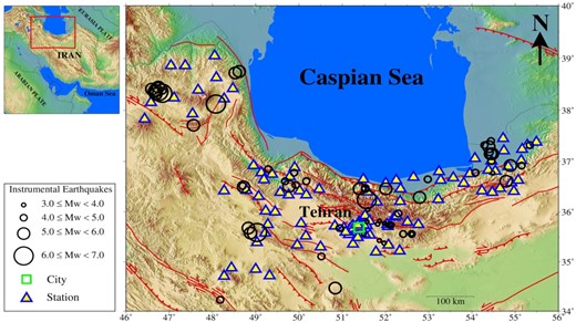
Map of Alborz region and adjacent area, epicenters of the considered earthquakes (circles) occurred during 1997–2019 and selected recording stations (triangles). Green square shows the location of Tehran.
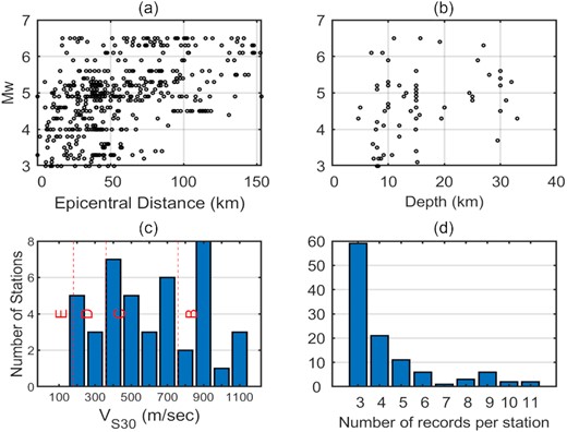
Plots showing, (a) magnitude–distance distribution of records in the data set, (b) magnitude–depth distribution of events, (c) distribution of station VS30 values and (d) number of stations against number of records per station. Vertical red dashed lines depict the limits of National Earthquake Hazard Reduction Program (NEHRP) site classes (E: soft soil; D: stiff soil; C: very dense soil and soft rock; B: rock).
The event-specific inverted moment magnitude (Mw) and stress parameter (|$\Delta {\rm{\sigma }}$|) values.
| Date | Earthquake ID | Lat. (N°) | Lon. (E°) | Magnitude | Inverted Mw | Δσ (MPa) | |${\kappa _0}$| (s) | N * | |||
|---|---|---|---|---|---|---|---|---|---|---|---|
| Mw | MN | Mb | ML | ||||||||
| 2019/11/07 | 201 901 | 37.71 | 47.56 | 5.9 | 5.8 | 4.32 | 0.016 | 4 | |||
| 2019/09/16 | 201 902 | 36.53 | 49.92 | 4.6 | 4.6 | 2.1 | 0.03 | 3 | |||
| 2018/02/09 | 201 801 | 35.43 | 51.86 | 3.6 | 3.8 | 1.9 | 0.036 | 9 | |||
| 2018/04/01 | 201 802 | 35.56 | 52.41 | 4.2 | 44 | 2.22 | 0.047 | 4 | |||
| 2018/09/22 | 201 803 | 36.65 | 52.98 | 3.3 | 4.8 | 5.35 | 0.033 | 6 | |||
| 2017/02/01 | 201 701 | 35.38 | 51.97 | 3.2 | 3.5 | 0.36 | 0.027 | 3 | |||
| 2017/04/28 | 201 702 | 35.76 | 51.82 | 3.4 | 3.5 | 4.42 | 0.01 | 18 | |||
| 2017/11/30 | 201 703 | 35.74 | 52.12 | 4.0 | 4.3 | 0.83 | 0.04 | 9 | |||
| 2017/12/20 | 201 704 | 35.68 | 50.95 | 4.9 | 5.1 | 8.59 | 0.043 | 34 | |||
| 2017/12/26 | 201 705 | 35.68 | 50.94 | 4.0 | 4.1 | 4.1 | 0.044 | 22 | |||
| 2016/02/01 | 201 601 | 35.81 | 51.57 | 3.1 | 3.4 | 7.69 | 0.022 | 5 | |||
| 2016/03/11 | 201 602 | 35.82 | 51.86 | 3.2 | 3.3 | 2.35 | 0.014 | 3 | |||
| 2016/04/17 | 201 603 | 35.75 | 52.04 | 3.4 | 3.6 | 0.67 | 0.025 | 6 | |||
| 2016/10/22 | 201 604 | 35.75 | 52.12 | 3.5 | 4.2 | 0.39 | 0.031 | 7 | |||
| 2015/05/10 | 201 501 | 36.78 | 49.89 | 4.3 | 4.5 | 1.67 | 0.033 | 3 | |||
| 2015/08/02 | 201 502 | 36.05 | 51.59 | 3.1 | 3.2 | 3.26 | 0.03 | 6 | |||
| 2015/08/25 | 201 503 | 35.56 | 52.59 | 4.5 | 4.8 | 3.91 | 0.03 | 21 | |||
| 2015/08/25 | 201 504 | 35.56 | 52.61 | 3.2 | 3.5 | 5.06 | 0.018 | 3 | |||
| 2015/09/15 | 201 505 | 37.32 | 54.29 | 4.3 | 4.9 | 11.62 | 0.029 | 4 | |||
| 2015/09/21 | 201 506 | 35.77 | 51.98 | 3.2 | 3.5 | 6.59 | 0.014 | 3 | |||
| 2014/08/16 | 201 401 | 35.97 | 52.3 | 4.1 | 4.8 | 1.5 | 0.044 | 3 | |||
| 2012/01/11 | 201 201 | 36.29 | 52.79 | 5.0 | 4.9 | 3.56 | 0.038 | 6 | |||
| 2012/08/11 | 201 202 | 38.33 | 46.84 | 6.5 | 6.0 | 5.57 | 0.023 | 7 | |||
| 2012/08/11 | 201 203 | 38.36 | 46.75 | 6.4 | 6.0 | 9.94 | 0.021 | 8 | |||
| 2012/08/11 | 201 204 | 38.26 | 46.76 | 3.4 | 3.6 | 1.62 | 0.026 | 5 | |||
| 2012/08/11 | 201 205 | 38.38 | 46.85 | 4.8 | 4.7 | 1.61 | 0.015 | 4 | |||
| 2012/08/11 | 201 206 | 38.32 | 46.69 | 5.2 | 4.9 | 1. 9 | 0.029 | 4 | |||
| 2012/08/11 | 201 207 | 38.36 | 46.66 | 5.2 | 5.1 | 3.36 | 0.022 | 4 | |||
| 2012/08/14 | 201 208 | 38.45 | 46.75 | 5.1 | 5.2 | 2.68 | 0.018 | 6 | |||
| 2012/08/14 | 201 209 | 38.38 | 46.7 | 5.0 | 5.1 | 1.73 | 0.025 | 4 | |||
| 2012/11/07 | 201 210 | 38.41 | 46.6 | 5.6 | 5.7 | 2.28 | 0.027 | 4 | |||
| 2011/08/11 | 201 101 | 36.61 | 54.79 | 4.9 | 5.1 | 8.08 | 0.046 | 4 | |||
| 2009/10/17 | 200 901 | 35.56 | 51.5 | 3.8 | 4.1 | 3.4 | 0.031 | 9 | |||
| 2008/05/27 | 200 801 | 36.5 | 48.72 | 5.0 | 4.9 | 10.38 | 0.034 | 7 | |||
| 2007/02/09 | 200 701 | 36.77 | 54.48 | 3.7 | 3.8 | 4.18 | 0.031 | 3 | |||
| 2007/05/11 | 200 702 | 36.85 | 49.29 | 4.3 | 4.3 | 0.86 | 0.03 | 3 | |||
| 2007/06/18 | 200 703 | 34.47 | 50.84 | 5.9 | 5.7 | 22.99 | 0.044 | 8 | |||
| 2007/07/11 | 200 704 | 38.75 | 48.62 | 5.2 | 5.0 | 2.71 | 0.005 | 3 | |||
| 2006/03/31 | 200 601 | 33.54 | 48.78 | 6.1 | 5.9 | 6.19 | 0.041 | 4 | |||
| 2005/01/10 | 200 501 | 37.15 | 54.47 | 5.3 | 5.5 | 45.71 | 0.035 | 22 | |||
| 2005/11/29 | 200 502 | 37.4 | 54.44 | 5.0 | 25.23 | 0.046 | 6 | ||||
| 2004/03/27 | 200 401 | 36.92 | 55.15 | 4.7 | 4.9 | 2.82 | 0.044 | 3 | |||
| 2004/05/28 | 200 402 | 36.25 | 51.57 | 6.3 | 6.1 | 14.00 | 0.035 | 24 | |||
| 2004/05/29 | 200 403 | 36.46 | 51.4 | 5.1 | 5.2 | 5.62 | 0.034 | 4 | |||
| 2004/05/30 | 200 404 | 36.45 | 51.53 | 4.2 | 4.7 | 2.45 | 0.038 | 3 | |||
| 2004/05/30 | 200 405 | 36.48 | 51.53 | 4.6 | 5.3 | 2.67 | 0.033 | 3 | |||
| 2004/10/07 | 200 406 | 37.15 | 54.43 | 5.6 | 5.7 | 86.7 | 0.037 | 22 | |||
| 2004/10/08 | 200 407 | 37.18 | 54.41 | 4.8 | 5.0 | 16.08 | 0.032 | 7 | |||
| 2003/09/12 | 200 301 | 37.32 | 55.32 | 4.6 | 5.0 | 12.6 | 0.037 | 3 | |||
| 2003/12/24 | 200 302 | 35.11 | 50.52 | 4.9 | 4.7 | 8.5 | 0.036 | 4 | |||
| 2002/04/08 | 200 201 | 36.46 | 52.01 | 4.6 | 5.2 | 2.27 | 0.036 | 5 | |||
| 2002/04/19 | 200 202 | 36.51 | 49.77 | 5.2 | 5.2 | 6.7 | 0.034 | 12 | |||
| 2002/04/19 | 200 203 | 36.61 | 49.68 | 4.4 | 4.5 | 1.55 | 0.039 | 5 | |||
| 2002/06/22 | 200 204 | 35.59 | 49.03 | 6.5 | 6.1 | 7.82 | 0.046 | 20 | |||
| 2002/06/22 | 200 205 | 35.58 | 48.88 | 5.0 | 5.2 | 1.53 | 0.043 | 4 | |||
| 2002/09/02 | 200 206 | 35.68 | 4.83 | 5.3 | 5.4 | 1.97 | 0.044 | 4 | |||
| 2000/08/16 | 200 001 | 37.01 | 54.45 | 4.9 | 5.1 | 14.35 | 0.036 | 8 | |||
| 1999/03/26 | 199 901 | 36.61 | 50.17 | 4.3 | 4.2 | 1.08 | 0.037 | 3 | |||
| 1999/11/19 | 199 902 | 37.29 | 54.39 | 5.5 | 5.5 | 64.92 | 0.038 | 12 | |||
| 1999/11/26 | 199 903 | 36.92 | 54.89 | 5.3 | 5.3 | 23.33 | 0.033 | 5 | |||
| 1998/07/09 | 199 801 | 38.72 | 48.53 | 5.9 | 6.0 | 7.22 | 0.019 | 7 | |||
| 1998/08/21 | 199 802 | 34.23 | 48.18 | 4.9 | 5.0 | 4.04 | 0.037 | 4 | |||
| 1998/09/28 | 199 803 | 36.52 | 48.7 | 4.6 | 4.6 | 5.39 | 0.039 | 5 | |||
| 1997/02/28 | 199 701 | 38.12 | 48.08 | 6.1 | 5.9 | 5.24 | 0.018 | 11 | |||
| 1997/09/16 | 199 702 | 36.78 | 54.08 | 4.8 | 5.0 | 20.42 | 0.031 | 3 | |||
N is the number of records.
PROCESSING OF STRONG MOTION RECORDS
We rotated longitudinal and transverse components to obtain the two orthogonal horizontal components northeast (H1) and east–west (H2) components. We also performed the base line correction that includes removing the mean and detrending any linear trend in the raw acceleration records. In order to identify the noise floor mainly at low frequency end of the spectrum, we performed signal-to-noise ratio (SNR) check for each record. The noise was extracted from the pre-event and post-event portion of the recorded time-history. The computed SNR estimates were then subsequently used to select the corner frequencies of filters used in the subsequent processing stage. We selected the high-pass filter corner frequency as the one for which the SNR becomes equal or larger than 3 (Boore & Bommer 2005). For majority of the recordings pre- and post-event noise was available; however, if for a record the selected noise window was smaller than 5 seconds then we chose a filter cut-off of 0.3 Hz. The low-pass filter corner frequency was computed for each component individually. The subsequent processing steps involve tapering of the time-series with a cosine taper to ensure zero levels on either ends of the time-history. We kept the taper window length 5 per cent (on each side) of the total signal length (Dawood et al. 2016). According to Boore (2005) to reduce the effect of the filter response, time-series are extended symmetrically at both ends with zero padding. Finally, we used two passes of Butterworth filter in the time domain with zero phase shift (Boore & Akkar 2003).
Fourier amplitude spectrum (FAS)
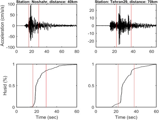
Plots showing the selection of the S-wave window from the acceleration time-series (horizontal components) of the 2004 Mw 6.2 Baladeh (Kojour) earthquake. Upper panels depict the selected S-wave window based on the time interval between the 3 and 80 per cent levels of the normalized Arias intensity (Arias 1970) (bottom panels).
METHODOLOGY
The inversion was performed in a single step (Oth et al. 2011) using the smoothed and rotational-independent average FAS of the ground motion over 40 frequencies from 0.3 to 30 Hz. The distance range is discretized into 73 bins of width 2 km. This discretization will allow us to estimate the frequency-dependent attenuation function in each distance bin. We used GIT to solve the system of linear equations, written in matrix form as |$Am\ = \ d$|, where d is data vector (i.e. logarithmic FAS), m is the model parameters vector, and A is a data kernel matrix. The overdetermined least square solution is given as, |${m^{est}} = {[ {{A^T}A} ]^{ - 1}}\ {A^T}d$|, where A–g =(ATA)–1 is the generalized inverse of A. The system of linear equations is solved in a least-squares sense (Paige & Saunders 1982) and we performed 200 bootstrap analyses (to evaluate the stability of the inversion) at each frequency point (Efron 1979; Parolai et al. 2000, 2004) and estimated the mean and standard deviation from these iterations (Jeong et al. 2020).
At each frequency, we have two unresolved degrees of freedom, that is, attenuation and the site. To address this issue, we need to add constraints in the inversion scheme. Two constrains were imposed in our inversion: (1) we fixed the attenuation term at a reference distance of 15 km, that is A(f,15) = 1 at each frequency. Consequently, the source functions will be representing earthquake source amplitudes at the selected reference distance; (2) to eliminate the trade-off between source and site amplification, we constrained the logarithm of the site amplification of the reference station (generally a rock site) to 0, irrespective of frequency. For selecting an appropriate reference station, we performed a preliminary inversion and also computed the HVSR to examine site transfer functions at all the stations. Our criteria for selecting the reference site were: (1) the inverted site amplification function should be close to 1 over the entire frequency range and (2) for that station the HVSR curve should also be flat over the entire frequency range and must not exhibit any significant peak (i.e. amplification >2). For the selected reference station (Hassan-Abad) that satisfies both of the above-mentioned criteria, the plots of site amplification function from preliminary inversion and HVSR curve are depicted in Fig. 4.
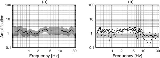
Site amplification for Hassan-Abad chosen as the reference station. (a) Amplification from a preliminary GIT inversion (solid black line and grey shaded area indicate bootstrap mean and ±1 bootstrap standard deviation of the estimated non-parametric site amplification functions from the GIT inversion technique, respectively) and (b) Amplification from HVSR analysis method (solid black line and thin dashed lines indicate mean and ±1 standard deviation).
RESULTS
Attenuation function
The non-parametric empirical attenuation functions obtained from inversions are depicted in Fig. 5 corresponding to different frequencies against hypocentral distance.
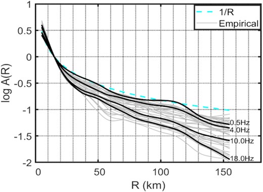
Variation of non-parametric (empirical) attenuation functions with distance in the Alborz region at all frequencies (solid light grey lines). Solid dark-grey lines indicate attenuation function at select frequencies (0.5, 4, 10 and 18 Hz) and the dashed line indicates 1/R amplitude decay.
In Fig. 6, the estimated geometrical spreading function determined from this study, a theoretical distance decay of |${\raise0.7ex\hbox{$1$} \!{/ {\vphantom {1 R}}} \!\lower0.7ex\hbox{$R$}}$| and, the Motazedian (2006) model are plotted with the empirical non-parametric functions (at different frequencies) to facilitate a graphical comparison. With such comparisons, we aim to evaluate the efficacy of derived geometrical spreading in capturing the apparent attenuation over a broad range of frequencies. We can clearly observe from Fig. 6 that the geometrical spreading function (eq. 8) derived from this study and that of Motazedian (2006) perform similar at near distances, while they are different at larger distances. As expected the match between geometrical spreading functions and the apparent attenuation functions is poorer towards higher frequencies, which can be attributed to frequency-dependent anelastic attenuation. Moreover, the high geometrical spreading rate at large distances obtained in this study is similar to the other studies for this region (Ahmadzadeh et al. 2019). Similar observations were made in southern Australia (Allen et al. 2007) where the apparent high geometrical spreading was attributed to the well-established velocity gradient in the region (Collins et al. 2003) that allows loss of Lg-wave energy into the mantle (e.g. Bowman & Kennett 1991; Atkinson & Mereu 1992).
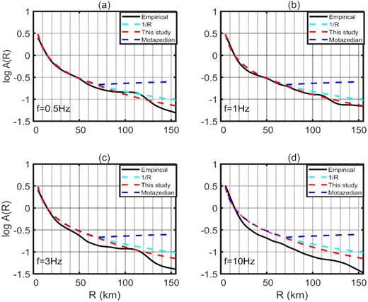
Comparison of the observed non-parametric attenuation functions with different distance decay models at frequencies (a) 0.5 Hz, (b) 1.0 Hz, (c) 3.0 Hz and (d) 10 .0 Hz.
Once, the geometrical spreading function is determined we keep it fixed for estimating the |$Q( f )$|. However, as mentioned earlier the geometrical spreading function and the anelastic attenuation functions are tied because of the way they enter into the model formulation (eq. 7). Thus, the estimation of |$Q( f )$| from the empirical attenuation functions is always dependent on the adopted geometrical spreading function. Therefore, in this study, we have estimated |$Q( f )$| by considering three cases of geometrical spreading function. We consider the theoretical geometrical spreading function for Swaves (1/R), bilinear (from this study) and the tri-linear hinged (Motazedian 2006) geometrical spreading model to correct the empirical (non-parametric) attenuation functions. To avoid the numerical instabilities (negative Q values) the fitting was performed in the distance range 21–100 km. The Q was determined at each frequency from the slope of least-squares regression line using |$Q( f )\ = {Q_0}\ {f^N}$| function, where Q0 and N are the regression coefficients. Fig. 7 depicts the fitting procedure and estimation of Q0 and N for the two cases: (i) the theoretical geometrical spreading function of |${\raise0.7ex\hbox{$1$} \!{/ {\vphantom {1 R}}} \!\lower0.7ex\hbox{$R$}}$| and (ii) the bilinear geometrical spreading function determined in this study. Final estimate of quality factor has been derived as |$Q\ ( f ) = {\rm{\ }}168{f^{0 \cdot 89}}$| (Fig. 7a) for the single decay geometrical spreading model and |$Q\ ( f ) = {\rm{\ }}146{f^{0 \cdot 91}}$| for the bilinear geometrical spreading model (Fig. 7b). For comparison purpose, we also used Motazedian (2006) geometrical spreading model and obtained the corresponding Q model as |$Q\ ( f ) = {\rm{\ }}93{f^{1 \cdot 02}}$|. From this analysis it is clear that the derived (average) Q model is strongly coupled with the adopted geometrical spreading function. Nevertheless, the derived quality factor values are not very different (statistically) given the uncertainty involved in their determination (Fig. 7).
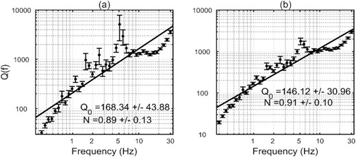
Q(f) model resulting from non-parametric attenuation function after fitting a frequency-dependent Q model along with the Q0 and N parameters, (a) for the 1/R geometrical spreading model and (b) for the bilinear geometrical model obtained from this study for Alborz region.
Table 2 presents a comparison of the derived Q models for Alborz region along with the Q-model derived in this study. The adopted geometrical spreading functions are also given along with the derived Qmodels in Table 2. Motazedian (2006) used 259 three-component strong-motion accelerograms recorded within northern Iran from 22 events in the magnitude range 4.9–7.4 and derived the quality factor as |$Q\ ( f ) = {\rm{\ }}87{f^{1 \cdot 46}}$|; this is similar to our estimated Q values using their geometrical spreading model. Zafarani et al. (2012) evaluated the quality factor as |$Q\ ( f ) = {\rm{\ }}101{f^{0 \cdot 8}}$| using the generalized inversion of the S-wave amplitude spectra from the strong-motion data in the Alborz region. Motaghi & Ghods (2012) used 136 earthquakes recorded at stations of the Institute of Geophysics of the University of Tehran during 1996–2007 in central Alborz mountains and reported a quality factor as |$Q\ ( f ) = {\rm{\ }}109{f^{0 \cdot 73{\rm{\ }}}}$|. Farrokhi & Hamzehloo (2017) by using the extended coda normalization method for 380 local earthquakes within frequency band 0.4–24 Hz, estimated the quality factors |$Q\ ( f ) = {\rm{\ }}83{f^{0 \cdot 99{\rm{\ }}}}$| and |$Q\ ( f ) = {\rm{\ }}68{f^{0 \cdot 96{\rm{\ }}}}$| for Alborz region and North Central Iran, respectively. Ahmadzadeh et al. (2019) used 312 crustal earthquakes recorded (1117 seismograms with ML 3–5.6) in the Alborz region between 2005 and 2017. They applied non-parametric spectral modelling of S-wave spectral amplitudes and estimated a quality factor model as|$\ Q\ ( f ) = {\rm{\ }}162{f^{0 \cdot 61{\rm{\ }}}}$| for a single decay model and |$Q\ ( f ) = {\rm{\ }}135{f^{0 \cdot 76{\rm{\ }}}}$| for a bilinear geometrical spreading model. The Q-model derived from this study is found to be similar to the models derived by Ahmadzadeh et al. (2019) and also, it is not very different from the models of Zafarani et al. (2012) and Motaghi & Ghods (2012). The Q-models determined by Motazedian (2006) and Farrokhi & Hamzehloo (2017) are different from the models derived in this study, which can be attributed to the difference in the underlying data set (Motazedian 2006) and to that the Farrokhi & Hamzehloo (2017) perform their analysis on the coda part of the records, while in the present study the S-wave window is used. Out of 65 events only 4 events are common between our study and the Motazedian (2006) (maximum 50 records).
Attenuation models for Alborz region.
| Reference | Q(f) | Geometrical spreading | Frequency range (Hz) |
|---|---|---|---|
| Motazedian (2006) | |$Q\ ( f ) = {\rm{\ }}87{f^{1 \cdot 46}}$| | $\left\{ \begin{array}{@{}*{1}{c}@{}} {{R^{ - 1}}\ \ \ \ \ R < 70}\\ {{R^{0 \cdot 2}}\ \ \ 70 \le R \le 150}\\ {{R^{ - 0 \cdot 1}}\ \ \ \ \ \ \ R >150} \end{array} \right. $ | |$1 < f \le 10$| |
| Zafarani et al. (2012) | |$Q\ ( f ) = {\rm{\ }}101{f^{0 \cdot 8}}$| | $\left\{ \begin{array}{@{}*{1}{c}@{}} {{R^{ - 1}}\ \ \ \ \ R < 70}\\ {{R^{0 \cdot 2}}\ \ \ 70 \le R \le 150}\\ {{R^{ - 0 \cdot 1}}\ \ \ \ \ \ \ R >150} \end{array} \right. $ | |$0.4 < f \le 15$| |
| Motaghi & Ghods (2012) | |$Q\ ( f ) = {\rm{\ }}109{f^{0 \cdot 73{\rm{\ }}}}$|. | $\left\{ \begin{array}{@{}*{1}{c}@{}} {{R^{ - 1.15}}\ \ \ \ \ R < 80}\\ {{R^{0 \cdot 09}}\ \ \ 80 \le R \le 160}\\ {{R^{ - 0 \cdot 5}}\ \ \ \ \ \ \ R >160} \end{array} \right. $ | |$0.6 \le f \le 12$| |
| Farrokhi & Hamzehloo (2017) | |$Q\ ( f ) = {\rm{\ }}83{f^{0 \cdot 99{\rm{\ }}}}$| | $\left\{ \begin{array}{@{}*{1}{c}@{}} {{R^{ - 1}}\ \ \ \ \ R < 90}\\ {{{( {90R} )}^{ - 0 \cdot 5}}\ \ \ \ \ \ \ R \ge 90} \end{array} \right. $ | |$0.4 < f \le 24$| |
| Ahmadzadeh et al. (2019) | Q |$( f ) = {\rm{\ }}162{f^{0 \cdot 61{\rm{\ }}}}$| | |${( {\frac{{{R_0}}}{R}} )^1}$| | |$0.3 < f \le 20$| |
| |$Q\ ( f ) = {\rm{\ }}135{f^{0 \cdot 76{\rm{\ }}}}$| | $\begin{array}{@{}*{1}{c}@{}} {{{( {\frac{{{R_0}}}{R}} )}^1}\ \ \ \ \ \ \ \ \ \ \ \ \ \ \ \ \ \ \ \ \ R < 70\ }\\ {{{( {\frac{{{R_0}}}{{60}}} )}^1}{{( {\frac{{60}}{R}} )}^{1.4}}.\ \ \ \ \ \ \ \ \ \ \ \ \ \ \ \ \ \ \ \ \ \ 70\ \le R \le 100\ } \end{array}$ | ||
| This study | Q |$( f ) = {\rm{\ }}168{f^{0 \cdot 89{\rm{\ }}}}$| | |${( {\frac{{{R_0}}}{R}} )^1}$| | |$0.3 \le f \le 30$| |
| Q |$( f ) = {\rm{\ }}146{f^{0 \cdot 91{\rm{\ }}}}$| | $\begin{array}{@{}*{1}{c}@{}} {{{( {\frac{{{R_0}}}{R}} )}^{1.01}}\ \ \ \ \ \ \ \ \ \ \ \ \ \ \ \ \ \ \ \ \ R < 70\ }\\ {{{( {\frac{{{R_0}}}{{70}}} )}^{1.01}}{{( {\frac{{70}}{R}} )}^{1.37}}.\ \ \ \ \ \ \ \ \ \ \ \ \ \ \ \ \ \ \ \ \ \ 70\ \le R \le 150\ } \end{array}$ |
Source spectra
In eq. (10) |${S_i}$| is the non-parametric source spectrum for ith event while |${\kappa _{0i}}$| is the corresponding |${\kappa _0}$| value and, |${f_E}$| is the lower limit of the frequency used for this fitting (i.e. frequency above which the decay is approximately linear on a plot of log Fourier amplitude versus linear frequency; Van Houtte et al. 2014). For our analysis |${f_E}$| was chosen either 10 or 15 Hz by visually inspecting each source spectrum. Subsequently, the estimated |${\kappa _0}$| was used to correct the high-frequency decay of the non-parametric source spectra. Fig. 8(a) shows an example of an uncorrected and |${\kappa _0}$|-corrected non-parametric source spectrum. Fig. 8(b) depicts distribution of |${\kappa _0}$| determined from each non-parametric source spectrum. The average |${\kappa _0}\ $| was found to be 0.032 s with the standard deviation of 0.01 s. Motazedian (2006) computed κ0 (represents the attenuation in the near-surface geology) for horizontal and vertical components equal to 0.05 and 0.03 s, respectively. Zafarani et al. (2012) estimated κ0 = 0.05 s for the horizontal and 0.02 s for the vertical components, respectively.
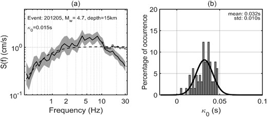
(a) Bootstrap mean (solid black line) and bootstrap standard deviation (grey shaded portion) of non-parametric source spectrum obtained from GIT inversion. The thin circled-line indicates the source spectrum after |${\kappa _0}$| correction applied on the frequencies beyond 10 Hz. (b) Distribution of |${\kappa _0}$| values obtained from the empirical non-parametric source spectra.
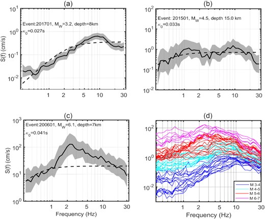
Panels (a), (b) and (c) represent |${\kappa _0}$| corrected non-parametric source spectrum (solid black line) in comparison with Brune's source model (dashed lines). The grey shaded area is the bootstrap standard deviation corresponding to each source spectrum. (d) Plots of |${\kappa _0}$| corrected non-parametric source spectrum for all events.
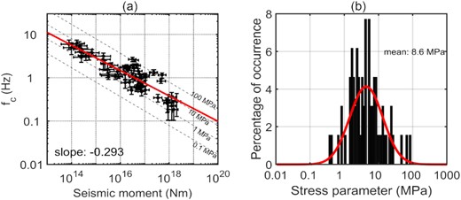
Plots showing, (a) corner frequency, fc, variations with seismic moment for Alborz earthquakes (constant stress parameter values (dashed lines) and slope of linear fit (solid red line) are also shown) and (b) distribution of stress parameters (|$\Delta \sigma $|).
Fig. 11 compares the inverted Mw (computed using source spectral fitting) with the database magnitude values. In Fig. 11(a), the original magnitude values at different scales are shown. Fig. 11(b) compares the inverted Mw values with the converted moment magnitudes using eqs (1), (2) and (3). The magnitude values from spectral fitting of source spectra show a good correlation with the database magnitude values for both cases, with a slight improvement when converting all magnitude scales into Mw. Fig. 12(a) shows the variation of the estimated |${\rm{\Delta }}\sigma $| values against the inverted Mw values. We also show |${\rm{\Delta }}\sigma $| values from Zafarani et al. (2012) for comparison. Clearly, the |${\rm{\Delta }}\sigma $| values exhibit a large scatter over the entire magnitude range and, we observed smaller stress parameter (<5 MPa) towards smaller magnitude (Mw < 4) events, while the |${\rm{\Delta }}\sigma $| values are larger towards larger magnitude. However, we do not prefer to propose a model for magnitude-dependence of |${\rm{\Delta }}\sigma $| owing to the lack of sufficient amount of data from higher magnitude-events (M > 6) in the region. Past studies conducted in this region also reported similar |${\rm{\Delta }}\sigma $| values and variability. Motazedian (2006) have also obtained average stress parameters of 12.5 MPa (Stochastic point-source) and 6.8 MPa (finite-fault modelling based on dynamic corner frequency) for earthquakes in North of Iran. Zafarani et al. (2012) estimated an average stress parameter values of 18.2 and 11.6 MPa, respectively for eastern and western Alborz region. Ahmadzadeh et al. (2019) calculated the stress parameter values range from about 0.02 to 16 MPa with an average of 1.1 MPa. Fig. 12(b) depicts the variation of the estimated |${\rm{\Delta }}\sigma $| values with focal depths. Although the scatter with depth is large, we see that the higher |${\rm{\Delta }}\sigma $| (>10 MPa) values are mainly associated with the deeper events. Owing to the large uncertainties in the reported focal depths, it is difficult to establish a well-constrained model of Δσ as a function of depth.
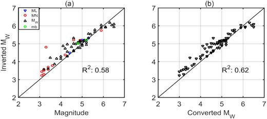
Comparison between the inverted magnitudes and the database magnitudes: (a) the original/reported magnitude values at different scales (b) different magnitudes scales are converted to moment magnitude scale.
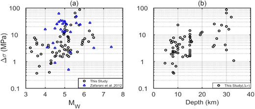
Stress-parameter (|$\Delta \sigma $|) values plotted against: (a) the inverted moment magnitude values from this study (black circles) and (b) the focal depth.
Site amplification functions
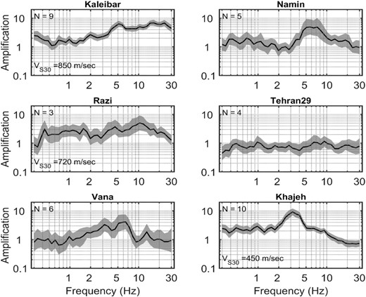
Bootstrap mean (solid black line) and ±1 bootstrap standard deviation (grey shaded area) of the estimated non-parametric site amplification functions at selected stations obtained from the GIT. N represents the number of records analysed at each station.
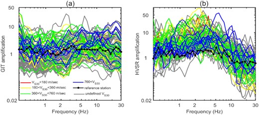
Plots showing: (a) estimated non-parametric site amplification functions at all stations obtained from the GIT inversion technique and (b) site amplification functions at all stations obtained from the HVSR method.
We computed the average station-specific HVSR at all the stations with more than three records. As mentioned earlier these station-specific HVSR curves are also used to identify a suitable reference (rock) station. A flat HVSR curve indicates a small or negligible impedance contrast between the sediments and the ‘seismological’ bedrock and thus no amplification of ground motion. In addition to the comparison shown in Fig. 14, Fig. 15 depicts comparison of GIT inverted site amplification functions and HVSR curves for some representative stations individually. At some of the stations such as Abgarm, Arjomand and Mamooniyeh the GIT site amplification curves and HVSR curves exhibit very good match, whereas at stations Eyvanaki1 and Lavasan1 the two curves do not match well. We also checked GIT site amplifications for the vertical components. For the stations where GIT and HVSR site amplification functions were comparable, there was no peak in the GIT site amplification for the vertical component. A similar observation was also made by Pacor et al. (2016) that when the GIT amplification function was flat for vertical component motion, the HVSR amplification function matches well with the GIT derived amplification functions. On the other hand, a non-uniform amplification on the vertical component indicates that two methods have a different shape and HVSR may not be a good indicator of SH site amplification amplitudes.
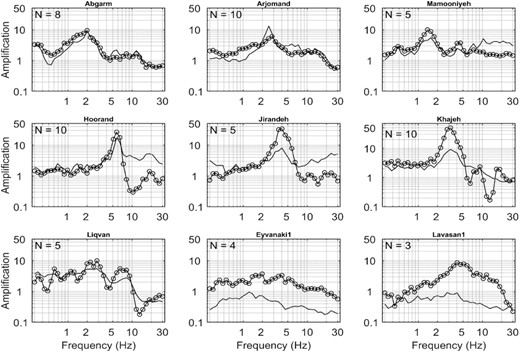
Comparison between GIT (solid line) and HVSR (circled line) site amplification functions for selected stations. N represents the number of records analysed at each station.
Furthermore, we compared the peak frequencies and the corresponding peak amplitudes of GIT inverted site amplification functions with those of HVSR curves at each station (Tsuda et al. 2010; Oth et al. 2011). For both the GIT and HVSR amplification functions we picked a global minimum and a global maximum in which the global maximum was accompanied by a local minimum on either side and all other local maxima. The criteria for selecting the peak frequency and the corresponding peak amplitude were: (1) amplitudes of all local maxima should be less than |${\raise0.7ex\hbox{$3$} \!{/ {\vphantom {3 4}}} \!\lower0.7ex\hbox{$4$}}$| of the global maximum, (2) the global minimum is smaller than the global maximum by a factor of five and (3) the amplitude of the global maximum is at least a factor of 2 larger than the amplitudes of the two local minima on either side. Fig. 16 compares peak frequencies and peak amplitudes determined by the two methods for all the stations in the data set. The peak frequencies from the two methods exhibit a better correlation than that for peak amplitudes. Although there is no consensus on whether HVSR amplitude represents the true site response, it is widely accepted that it is being able to adequately capture the resonance peak |${f_0}$| (Fäh et al. 2001).
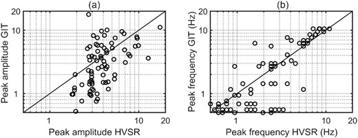
Comparisons between peak amplitudes (a) and peak frequencies (b) determined from GIT and H/V methods.
Robustness evaluation of spectral model parameters
The robustness of the spectral model parameters used to parametrize the source spectra |$S( f )$| including stress parameter and inverted moment magnitude, and also the attenuation function |$A( {f,\ r} )$| is evaluated in two ways: (1) visual comparison between the observed and predicted spectra at selected stations and (2) residual analysis. Fig. 17 depicts comparison between the modelled and observed spectra for a selected set of events and station combinations. The source spectra are modelled by assuming an ω-squared model with seismic moments |${M_0}$| estimated from the inversion. The frequency-dependent attenuation function is described by eq. (7), in which the geometrical spreading function is given in eq. (8), and the corresponding quality factor is |$Q\ ( f ) = {\rm{\ }}146{f^{0 \cdot 91}}$|. The forward model predictions were made for two cases of the ω-squared source model, (i) event-specific corner-frequency |${f_c}$| and (ii) |${f_c}$| corresponding to an average stress parameter |$\Delta \sigma \ = \ 8.6$| MPa. In general, the model predicted spectra matched reasonably well with the observed spectra and, as expected the match improves when event-specific |${f_c}$| values are used for the ω-squared source model. However, in practice |$\Delta \sigma $| values of future earthquakes are not known a priori. Hence, it is common practice to use the average stress parameter in such cases. It should also be noted that the forward model predictions shown here are made with an assumption that the source spectrum of an earthquake can be modelled by a single-corner omega-square model.
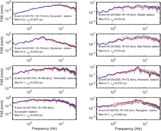
Comparison between the observed and modelled (using the model parameters derived in this study) FAS. Thin grey curves are showing the observed (average of two horizontal components) spectra at the selected stations. The modelled FAS using the event-specific stress parameter, |$\Delta \sigma $|, and the average stress parameter |$\Delta \sigma = \ 8.6$| MPa, are shown with red thick and blue dashed lines, respectively.
To further evaluate the goodness-of-fit of our non-parametric inverted models, we plotted the residuals against magnitude and distance in Fig. 18 at selected frequencies representing low and high-frequency portion of the spectrum. The residuals are calculated as the difference between the logarithms of the observed spectral amplitudes and the predicted target amplitudes. The predicted values are computed using the non-parametric source, path and site functions. The computed residuals do not show any trend with magnitude and distance and, they are randomly scattered around the center line of zero. It is concluded that, the performed non-parametric inversion provides representative empirical functions for source, path and site effects for the selected data set. The results also indicate robustness of the estimated seismological parameters (e.g.|$\ {M_0}$|, |$\Delta \sigma $|, geometrical spreading function and Q model) from the non-parametric empirical functions.
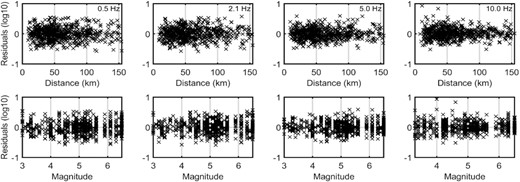
Variation of the residuals with hypocentral distance (top panel) and magnitude (below panel) for 0.5, 2.1, 5.0 and 10.0 frequencies.
CONCLUSIONS
In this study, we analysed 478 three-component strong ground motion records from 65 events (Mw 3–6.5) recorded over 111 stations at hypocentral distances |$R \le 150$| km in the Alborz region of northern Iran since 1997. Strong ground motion records are processed following standard protocols, and different magnitude types are converted to a unified moment magnitude to obtain a homogenized catalogue. Fourier spectral amplitudes are computed for the S-wave window of the acceleration time-series. The smoothed Fourier spectral amplitudes at 40 frequencies equally spaced on a log scale are used to estimate non-parametric source, path and site functions using the GIT. Seismological parameters including stress parameter, seismic moment, moment magnitude, geometrical spreading and anelastic attenuation functions are estimated from the non-parametric spectral functions. Major findings from our analysis can be summarized as follows:
The non-parametric empirical attenuation functions were modelled as a combination of frequency-independent geometrical spreading and frequency-dependent anelastic attenuation function. The geometrical spreading function is described by a bilinear piecewise function with a transition distance at 70 km (eq. 8). Motazedian (2006) proposed a trilinear piecewise geometrical spreading function for the same region. The geometrical spreading function derived in this study is simple yet powerful enough to capture the observed trend in the data. Also, the transition distance of 70 km was selected by trial and error method performed over a set of transition distances between 30 and 100 km with an interval of 10 km. The quality factor associated with the bilinear geometrical spreading function was found to be |$Q\ ( f ) = \ 146\ {f^{0.91}}$|. The corresponding quality factor for a theoretical geometrical spreading function of 1/R is |$Q\ ( f ) = \ 168\ {f^{0.89}}$|.
The ω-square single corner source model was found suitable in explaining most of the non-parametric empirical source spectra. The empirical source spectra were first corrected for a high-frequency decay at frequencies beyond 10 Hz. This high-frequency decay was attributed to the |${\kappa _0}$| with an average value (horizontal component) of 0.032 s and standard-deviation of 0.01 s. Although, the exact physical origin of |${\kappa _0}$| is not yet known, we attribute the values determined here with source component of kappa (Papageorgiou & Aki 1983; ; Papageorgiou 1998; Oth et al. 2011; Kilb et al. 2012; Bindi et al. 2017; Ji et al. 2020).
Fitting of an ω-squared source model to |${\kappa _0}$|-corrected empirical source spectra resulted in two source parameters namely seismic moment |${M_0}$| and corner frequency (|${f_c}$|) for each event. The |${M_0}$| values were converted to obtain event-specific moment magnitudes Mw. The inverted Mw were found in good agreement with the magnitude values given in the database. This indicates robustness of the inverted Mw values as well as, that the adequacy of the single-corner ω-squared model to explain the empirical source spectra.
The corner frequency |$( {{f_c}} )$| and the inverted Mw values were used to estimate the Brune's stress parameter (|$\Delta \sigma $|). We observed large variability in |$\Delta \sigma $| but, we did not find a significant dependence of |$\Delta \sigma $| with magnitude. The |$\Delta \sigma $| values in the data set range from 0.36 to 86.7 MPa with an average value of |$\Delta \sigma \ = \ 8.6$| MPa. The |$\Delta \sigma $| values obtained in this study were found comparable with the values obtained from other studies for the study region. Furthermore, the higher |$\Delta \sigma $| values were found to be associated with deeper earthquakes.
The GIT site amplification functions obtained were found to exhibit large station-to-station variability, though we did not observe significant regional pattern in site-amplification functions. We observed a good match between GIT amplification functions and the HVSR curves over some stations. At those stations, a smaller and uniform amplification in the vertical component was found over the entire frequencies range. For stations with high amplification in vertical component, the match between GIT amplification and HVSR curves was found to be poorer.
We tested the robustness of the proposed spectral models herein by comparing the model predicted spectra with the observed spectra for some event and station combinations. Models with event-specific |$\Delta \sigma $| were found to perform better in comparison to an average |$\Delta \sigma $| of 8.6 MPa. From forward prediction perspective, we envisage that the spectral models derived in this study are valid within the magnitude range Mw 3–6.5 and up to a distance of 150 km. Although the models derived in this study are of semi-empirical nature with physics-based ω-squared source model, an extrapolation of the parameters beyond the magnitude and distance range prescribed here must be validated vis-à-vis observed ground motions.
ACKNOWLEDGEMENTS
This work was financially supported by University of Tehran. First author, Mehran Davatgari Fami Tafreshi thanks IIT Gandhinagar for hosting him and providing all the necessary support. The authors also acknowledge the Building and Housing Research Center of Iran for generously providing the data for this work. We also thank Adrien Oth for helping with the technical details related to his GIT code and Saeid Rahimzadeh for his help in preparing Fig. 1. The authors also thank reviewers Daniel Garcia, Carlos Ortiz-Aleman and the editor Prof Victor M. Cruz-Atienza for their constructive comments and feedback, which has helped to improve the paper.
DATA AVAILABILITY
Ground motion records used in this study are accessible at the website of Building and Housing Research Center (BHRC) of Iran (http://www.bhrc.ac.ir/), last accesed February 2020. The derived data generated in this research will be shared on reasonable request to the corresponding author.
