A global reference model of the lithosphere and upper mantle from joint inversion and analysis of multiple data sets

Afonso, Juan Carlos; Salajegheh, Farshad; Szwillus, Wolfgang; Ebbing, Jorg; Gaina, Carmen

doi:10.1093/gji/ggz094

SUMMARY

We present a new global model for the Earth’s lithosphere and upper mantle (LithoRef18) obtained through a formal joint inversion of 3-D gravity anomalies, geoid height, satellite-derived gravity gradients and absolute elevation complemented with seismic, thermal and petrological prior information. The model includes crustal thickness, average crustal density, lithospheric thickness, depth-dependent density of the lithospheric mantle, lithospheric geotherms, and average density of the sublithospheric mantle down to 410 km depth with a surface discretization of 2° × 2°. Our results for lithospheric thickness and sublithospheric density structure are in excellent agreement with estimates from recent seismic tomography models. A comparison with higher resolution regional studies in a number of regions around the world indicates that our values of crustal thickness and density are an improvement over a number of previous global crustal models. Given the strong similarity with recent tomography models down to 410 km depth, LithoRef18 can be readily merged with these seismic models to include seismic velocities as part of the reference model. We include several analyses of robustness and reliability of input data, method and results. We also provide easy-to-use codes to interrogate the model and use its predictions for the development of higher-resolution models.

Considering the model‘s features and data fitting statistics, LithoRef18 will be useful in a wide range of geophysical and geochemical applications by serving as a reference or initial lithospheric model for (i) higher-resolution gravity, seismological and/or integrated geophysical studies of the lithosphere and upper mantle, (ii) including far-field effects in gravity-based regional studies, (iii) global circulation/convection models that link the lithosphere with the deep Earth, (iv) estimating residual, static and dynamic topography, (v) thermal modelling of sedimentary basins and (vi) studying the links between the lithosphere and the deep Earth, among others. Several avenues for improving the reliability of LithoRef18’s predictions are also discussed. Finally, the inversion methodology presented in this work can be applied in other planets for which potential field data sets are either the only or major constraints to their internal structures (e.g. Moon, Venus, etc.).

Composition and structure of the continental crust, Composition and structure of the mantle, Gravity anomalies and Earth structure, Satellite gravity, Planetary interiors, Seismic tomography

1 INTRODUCTION

Global models of the physical state and properties of the Earth’s interior have improved considerably over the past decade due to the availability of higher-quality and more comprehensive data sets, the rapid growth in computational and data processing power, new developments in both theoretical and experimental mineral physics at high pressure and temperature conditions and the arrival of new satellite-derived datasets of global coverage (e.g. GRACE and GOCE missions). Such models, especially those focused on the lithosphere and upper mantle, have proven useful in a wide range of geophysical and geodynamic applications. They are needed for stripping off, or accounting for, crustal effects in seismic tomography studies (the so-called crustal correction; e.g. Waldhauser et al.2002; Chang & Ferreira 2017), as reference or starting models in regional gravity and/or isostatic studies (e.g. Mechie et al.2013; Levandowski et al.2014; Aitken et al.2015), as input in global circulation/convection models and dynamic topography studies (e.g. Flament et al.2013; Becker et al.2014; Steinberger 2016), as anchor points in the interpretation of a number of geochemical data (cf. Rudnick & Gao 2003; Hawkesworth et al.2016) and as input or constraints in evolutionary models of basins (cf. Wangen 2010), to name a few. In their own right, global models of the Earth’s internal structure and physical parameters help in addressing fundamental questions about the nature and evolution of continents, the nature of mantle convection, the coupling between lithospheric plates and sublithospheric mantle and the roles of crust vs mantle in the evolution of topography, among others.

Despite their obvious importance, global models of the Earth’s interior that honour multiple data types (i.e. seismic, gravity, geoid, magnetotelluric, etc.) are still rare. This is a significant limitation because data gathering at the required scale is expensive and different data sets offer crucial complementary information. Moreover, it is well-known that models constrained by single data sets typically fail at providing satisfactory fits to other observables (e.g. Forte et al.2007; Afonso et al.2013b, 2016a). A few whole-mantle global models that are compatible with more than one data type (not only seismic) are available, albeit at relatively low resolutions (e.g. Ishii & Tromp 1999; Forte et al.2009; Simmons et al.2006, 2010; Cammarano et al.2011; Wang et al.2015; Yang & Gurnis 2016; Greff-Lefftz et al.2016a). Of particular relevance is the whole-mantle model of Simmons et al. (2010), in which multiple seismic and geodynamic observables are inverted and linked through empirical mineral-physics parameters. Despite being one of the most advanced approaches to date, lithospheric density structure was not the focus of that study, as indicated by the modelling assumptions and datasets used.

The recent model LITHO1.0 (Pasyanos et al.2014), based on Love and Rayleigh wave data (group and phase) is an extension of the popular crustal model CRUST1.0 (Laske et al.2013). It is a 1° tesselated model containing estimates of crustal velocity, density and thickness, as well as upper mantle velocity, lithospheric thickness, and mantle density (albeit an unrealistic one). Given its resolution and the fact that it is based on surface wave data and an a priori crustal model calibrated with gravity and seismic data, LITHO1.0 is an attractive candidate as a reference model for the shallow structure of the Earth. However, its density structure and boundaries’ geometry have not been optimized to satisfy potential field data and the proxy used to estimate lithospheric thickness (strictly, the thickness of a constant-velocity seismic lid) is likely to result in under and overestimation of the lithosphere-asthenosphere boundary (LAB) beneath thin and thick continental lithosphere, respectively. Conversely, a number of global density models for the crust and upper mantle have been obtained from modelling or inversion of either gravity, geoid, gravity gradients or some combination of them (e.g. Kaban et al.2004; Reguzzoni et al.2013; Reguzzoni & Sampietro 2015; Sampietro 2016; Sjöberg & Bagherbandi 2011), with limited or no formal input from seismic studies (note that regional models that combine both seismic and gravity data are more common, e.g. Maceira & Ammon 2009; O’Donnell et al.2011; Shan et al.2014; Afonso et al.2016c; Tondi et al.2017). However, most of these ‘gravity-based’ models are crustal models only. There is therefore an ambiguity regarding which model is more suitable as a global reference for lithospheric/upper mantle studies in the context of integrated studies or joint inversions making use of multiple data sets (e.g. Zeyen et al.1997; Tiberi et al.2008; Moorkamp et al.2011; O’Donnell et al.2011; Fullea et al.2015; Shan et al.2014; Afonso et al.2016c; Tork Qashqai et al.2016; Tondi et al.2017; Syracuse et al.2017, among many others).

In this paper, we present a global model of the lithosphere and sublithospheric upper mantle obtained via an iterative nonlinear joint inversion scheme of gravity anomalies, geoid height, satellite-derived gravity gradients and absolute elevation. These datasets were chosen due to their different and complementary depth sensitivities to density anomalies. First-order seismic, petrological and geothermal prior information is also included in the inversion. The model and inversion are developed in spherical coordinates with a lateral discretization of 2° × 2°. A massively-parallel implementation of the inversion algorithm was necessary given the size of the system of equations and the large number of model parameters resulting from the model discretization. Relevant (prior) seismic information is included by adopting CRUST1.0 (Laske et al.2013) and a LAB model based on six recent seismic tomography models (cf. Pasyanos et al.2014; Steinberger 2007) as prior models, which are modified only slightly during the inversion as required by the data.

We have prepared user-friendly codes to extract information from the model, including the computations of contributions from the entire model (or parts of it) to gravity, geoid and gravity gradients at any point on or above the surface of the planet; this is particularly useful when dealing with the so-called far-field/edge/boundary effects in gravity-related studies. The model contains average crustal density, crustal thickness, lithospheric thickness, depth-dependent density of the lithospheric mantle, lithospheric geotherms, and average density of the sublithospheric mantle down to 410 km depth. These outputs are expanded by including seismic velocities from a compatible tomography model (SL2013sv; Schaeffer & Lebedev 2013). Given its characteristics, we expect that this model will be useful to the broader community by serving as a reference/initial model for (i) higher-resolution gravity, seismological, geodetic and/or integrated geophysical studies of the lithosphere and upper mantle, (ii) including far-field effects in regional gravity/geoid studies, (iii) regional and global geodynamic simulations where lithospheric thickness and structure plays a non-negligible role, (iv) assessing isostatic compensation mechanism and estimates of residual, isostatic and dynamic topography, (v) stripping off the lithospheric signal in global and regional estimates of the deep structure of the Earth and (vi) estimating boundary conditions for thermal modelling of sedimentary basins, among others.

In what follows, we begin by discussing the input data sets (Section 2), the solution to the forward problems (Section 3), the treatment of temperature-, pressure- and composition-dependent parameters (Section4) and the discretization of the model (Section 5). We continue with the description of the general inversion strategy (Section 6) and present results from illustrative synthetic tests. The final model and main results are presented in Section 8. Finally, we discuss some relevant features of the model and possible future improvements in Section 9. Appendices A and B provide additional information on the parallel implementation of the inversion scheme and on the global resolution matrix, respectively.

2 INPUT DATA SETS AND INITIAL MODEL

Elevation data were taken from the 1 × 1 arcmin global model ETOPO1, which combines land topography and ocean bathymetry (Amante & Eakins 2009); the model is available at https://www.ngdc.noaa.gov/mgg/global/. Free-air gravity anomalies were taken from the global gravity model WGM2012 (Balmino et al.2012,http://bgi.omp.obs-mip.fr). Gravity gradients are provided by the satellite mission GOCE (Pail et al.2017). In particular, we used the satellite-only global Earth model GOCO03S (http://www.goco.eu/) and computed the full Marussi tensor up to degree and order 250 at satellite height using a spherical harmonics synthesis code (Fullea et al.2015). Geoid heights are taken from the global model EGM2008 (Pavlis et al.2012); note that model WGM2012 is in principle compatible with both ETOPO1 and EGM2008.

Since the focus of this study is the upper ∼410 km of the Earth, we need to filter the total geoid by removing low orders and degrees (i.e. long wavelengths), which are thought to be largely controlled by deep density anomalies. To this end, we used the tapering approach of Marks et al. (1991) to minimize Gibbs oscillations in the residual (filtered) geoid. Based on previous studies (e.g. Hager 1984; Doin et al.1996; Featherstone 1997; Chase 1985; Bowin 1983, 2000; Chase et al.2002; Golle et al.2012) and numerous tests (see Supporting Information), we chose to roll off spherical harmonic coefficients between degrees 8 and 12 using a cosine tapering function. To keep consistency between data sets, the same filtering approach was applied to gravity and gravity gradients data. Further details on the effects of the geoid filtering on the final results are given in Section 7.2 and in Supporting Information.

An important set of ‘input data’ are those used to construct the initial/starting model and priors for the crust and lithosphere. The initial model for crustal thickness and density is based on the well-known global model CRUST1.0 (Laske et al.2013), whereas the initial lithospheric thickness is obtained from a hybrid model based on six recent global tomography models: LITHO1.0 (Pasyanos et al.2014), SAVANI (Auer et al.2014), SL2013sv (Schaeffer & Lebedev 2013), GYPSUM (Simmons et al.2010), S40RTS (Ritsema et al.2011) and SEMUM2 (French & Romanowicz 2014). Five of these models have been recently reviewed by Steinberger & Becker (2016), who proposed a procedure to derive consistent estimates of (thermal) lithospheric thickness from these models. Since the predicted LAB from all these models are comparable and highly correlated, we opted for a compromise hybrid LAB model that is a weighted average of all six tomography models. Considering the actual features of these models (e.g. type of data, depth range of interest, resolution, etc.), we assign the largest weights to LITHO1.0 and SL2013sv. The actual starting LAB model so obtained is introduced in Section 8.2 and shown in Fig. 8 A.

In the oceans, we choose not to use the original LAB depths provided by the above models as some of them contain a number of dubious regions with unrealistically high values. Instead, our initial LAB model is based on a plate cooling model (Grose & Afonso 2013), which has been constrained by bathymetric, surface heat flow, petrological and mineral physics data. To use this model, the age of the oceanic crust is needed, which we take from Müller et al. (2008).

Given the lack of well-constrained density models for the sublithospheric upper mantle, we choose to start with a constant density in this part of the model and let the inversion to modify it according to the data fit statistics. Based on results from preliminary inversions and synthetic tests, we select ρ_a = 3450 kg m⁻³ for the initial sublithospheric density; this value is very close to the horizontally averaged value of the preliminary inversions and results in good convergence performance during the inversion, good data fit statistics and realistic density values (Section 8).

3 FORWARD PROBLEMS

3.1 Gravity, geoid and gravity gradients

For most geophysical purposes, the spherical approximation to computing gravity signals (as opposed e.g. to the elliptical approximation) yields results of sufficient accuracy (e.g. Novak & Grafarend 2005; Asgharzadeh et al.2007). Considering geographical coordinates, the so-called spherical tesseroid represents a natural mass element for subdividing a spherical Earth (cf. Anderson 1976; Grüninger 1990; Heck & Seitz 2007). A spherical tesseroid is a body bounded by two concentric spheres of radii r₁ and r₂, two meridional planes defined by longitudes λ₁ and λ₂, and two parallels (or coaxial cones) with latitudes φ₁ and φ₂ (See Fig. 1 A)

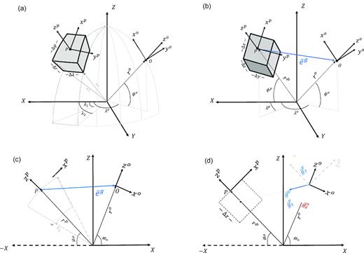
$(a) Geometry of a spherical tesseroid showing global (X, Y, Z) and local (xp, yp, zp; xo, yo, zo) coordinate systems. (b) Prism approximation of a tesseroid. (c–d) 2-D view of a right rectangular prism approximating a tesseroid. The geometric relationship between vectors $\overline{e}^p$, $\overline{e}^{g}$, $\overline{g}^{o}$ and $\overline{g}^{g}$are shown.$

Figure 1.

(a) Geometry of a spherical tesseroid showing global (X, Y, Z) and local (x^p, y^p, z^p; x^o, y^o, z^o) coordinate systems. (b) Prism approximation of a tesseroid. (c–d) 2-D view of a right rectangular prism approximating a tesseroid. The geometric relationship between vectors |$\overline{e}^p$|⁠, |$\overline{e}^{g}$|⁠, |$\overline{g}^{o}$| and |$\overline{g}^{g}$|are shown.

Open in new tab Download slide

The gravitational potential V at observation point O(r^o, φ^o, λ^o) produced by a spherical tesseroid with constant density ρ is given by Netwon’s integral in spherical coordinates (cf. Heck & Seitz 2007)

\begin{eqnarray*} V\left(r,\varphi ,\lambda \right) = G\rho \int \limits _{\lambda _{1}}^{\lambda _{2}}\int \limits _{\varphi _{1}}^{\varphi _{2}}\int \limits _{r_{1}}^{r_{2}} \dfrac{(r^{p})^2\cos \varphi ^{p}dr^{p}d\varphi ^{p}d\lambda ^{p}}{\ell } , \end{eqnarray*}

(1)

where

\begin{eqnarray*} \ell \left(P,O\right) = \sqrt{(r^o)^{2}+(r^p)^{2}-2r^or^p\, \cos \Psi } \end{eqnarray*}

(2)

is the Euclidean distance between the computation point O(r^o, φ^o, λ^o) and the integration point P(r^p, φ^p, λ^p); Ψ is the angle between the position vectors of O and P (Figs 1 A and B), given by

\begin{eqnarray*} \cos \Psi = \sin \varphi ^o\, \sin \varphi ^p+\cos \varphi ^o\, \cos \varphi ^p\, \cos \left(\lambda ^o-\lambda ^p\right). \end{eqnarray*}

(3)

Eq. (1) is an elliptic-type integral and has no closed-form analytical solution. A number of numerical methods in the spatial domain are available to approximate eq. (1). Among these, those based on Taylor series expansions and/or Gauss–Legendre quadrature rules are the most popular (e.g. Heck & Seitz 2007; Grombein et al.2013; Wild-Pfeiffer 2008; Asgharzadeh et al.2007). Despite generally yielding the most efficient solutions (especially at planetary scale), spectral or frequency-domain methods based on spherical harmonic expansions seem to be less common due to the cumbersome formulation for representing highly variable and/or discontinuous density distributions and the need to account for additional technical considerations (e.g. spectral coherency, global mass distributions, resolution-dependent convergence issues, etc.; Kuhn & Featherstone 2005; Kuhn & Seitz 2005; Balmino et al.2012; Hirt & Kuhn 2014).

Spatial methods that solve eq. (1) directly (by e.g. quadrature rules or Taylor expansions) provide efficient and accurate results at relatively high elevations above the tesseroid, making them the preferred options when modelling satellite data. However, they are not well-suited for computing the potential (and its derivatives) near, at, or below the surface of the tesseroid. This creates a problem when the surface of the planet is discretized with tesseroids and terrain corrections or gravity values from land surveys need to be modelled (Grombein et al.2013).

3.1.1 The prism approximation

A popular alternative to solving eq. (1) directly is to approximate the tesseroids with rectangular prisms having the same mass and height as the tesseroids (e.g. Anderson 1976; Grüninger 1990; Kuhn 2000; Heck & Seitz 2007; Wild-Pfeiffer 2008). This is advantageous not only because analytical solutions for flat-topped rectangular prisms are available, but also because it is possible to obtain solutions at or near the top of the prism or even inside it (by appropriate splitting). The validity and accuracy of this approximation rely on three conditions: (1) that the surface area of the tesseroids are sufficiently small so a flat-topped prism offers an acceptable approximation, (2) that we have prisms/tesseroids that are not too long along their vertical dimension and (3) that both mass elements have the same mass. If the first condition is not guaranteed, a flat-topped prism will not be a good approximation of the tesseroid (i.e. the curvature of the tesseroid’s surface plays a significant role). If the second condition is not met, the shape of the prism will depart from that of tesseroid which is trying to approximate (Fig. 1C). Consequently, even when the third condition is met (see below), the results of the prism approximation will depart from the correct one. In practice, the surface area of the tesseroids depend on the actual application, but a number of tests (see Supporting Information) indicate that even in the unfavourable case of a tesseroid with dimensions 2° × 2° × 100 km depth, the maximum errors for geoid, gravity and gravity gradients produced with the prism approximation are 0.6, 0.5 and 1.3 per cent, respectively, for observations points within 500 km from the tesseroid.

Throughout this work, we adopt the prism approximation. We acknowledge that for global studies, spectral methods would offer a more efficient solution. However, we are interested in a formulation general enough to allow us to model a large range of scales (local, regional, global), highly variable density distributions, with no singularities at the surface or within the mass bodies, and importantly, that allows to obtain fast solutions of small density perturbations (e.g. by changing the density of one prism inside the model). These requirements are readily met by the prism approximation and are critical for forthcoming studies based on joint probabilistic inversions (e.g. Afonso et al.2013b,a, 2016a,c).

There are two main ingredients in the prism approximation. First, a complete set of analytical solutions for a rectangular prism is needed to compute the potential of each prism in Cartesian coordinates. Secondly, a set of coordinate transformations is required to compute the correct vector components in spherical coordinates (account for the convergence of the plumb line). The formulae associated with the computation of the gravity potential and its derivatives for a rectangular prism are well-known and described in detail elsewhere (cf. Mader 1951; Nagy et al.2000; Gallardo-Delgado et al.2003; Fullea et al.2009, 2015); therefore, we do not repeat them here. In the following, we describe the process of coordinate transformation and conservation of mass between the mass elements.

The formulae for gravity, geoid and gravity gradients, for instance those in Nagy et al. (2000), Fullea et al. (2009, 2015), assume that the observation point is at the origin of a Cartesian coordinate system and the edges of the causative prism are parallel to the coordinate axes. Therefore, referring to Figs 1(B) and (C), we must convert the vector |$\overline{e}^g$| from the global Cartesian coordinates associated with the terrestrial equatorial reference frame (X, Y, Z) to the local coordinates of the prism |$\overline{e}$| (x^p, y^p, z^p). We first obtain |$\overline{e}^g$| from its spherical coordinate components

\begin{eqnarray*} \overline{e}^{g} = \begin{bmatrix}r^{o}\cos \phi ^{o}\cos \lambda ^{o}\\ r^{o}\cos \phi ^{o}\sin \lambda ^{o}\\ r^{o}\sin \phi ^{o} \end{bmatrix}- \begin{bmatrix}r^{p}\cos \phi ^{p}\cos \lambda ^{p}\\ r^{p}\cos \phi ^{p}\sin \lambda ^{p}\\ r^{p}\sin \phi ^{p} \end{bmatrix} . \end{eqnarray*}

(4)

Now we can transform |$\overline{e}^g$| into the local coordinates of the prism |$\overline{e}^p$| by applying two rotations and a reflection operation

\begin{eqnarray*} \overline{e}^p = {\bf P}_y \, .\, {\bf R}_{y}(90^{\text{$\circ $}}-\phi ^{p}) \, .\, {\bf R}_{z}(180^{\text{$\circ $}}-\lambda ^{p}) \, .\, \overline{e}^{g} , \end{eqnarray*}

(5)

where R_y and R_z are the Euler rotation matrices around the y- and z-axes, respectively, and P_y is a reflection matrix needed to correct for the different polarity of the local and global reference frames. The explicit forms of these matrices are (cf. Grüninger 1990; Torge 2001)

\begin{eqnarray*} {\bf P}_{y} = \begin{bmatrix}1 & \quad 0 & \quad 0\\ 0 & \quad -1 & \quad 0\\ 0 & \quad 0 & \quad 1 \end{bmatrix} \end{eqnarray*}

(6)

\begin{eqnarray*} {\bf R}_{y}\left(90^{\text{$\circ $}}-\phi ^{p}\right) = \begin{bmatrix}\cos \left(90^{\text{$\circ $}}-\phi ^{p}\right) & \quad 0 & \quad \sin \left(90^{\text{$\circ $}}-\phi ^{p}\right)\\ 0 & \quad 1 & \quad 0\\ -\sin \left(90^{\text{$\circ $}}-\phi ^{p}\right) & \quad 0 & \quad \cos \left(90^{\text{$\circ $}}-\phi ^{p}\right) \end{bmatrix} \end{eqnarray*}

(7)

\begin{eqnarray*} {\bf R}_{z}\left(180^{\text{$\circ $}}-\lambda ^{p}\right) = \begin{bmatrix}\cos \left(180^{\text{$\circ $}}-\lambda ^{p}\right) & \quad -\sin \left(180^{\text{$\circ $}}-\lambda ^{p}\right) & \quad 0\\ \sin \left(180^{\text{$\circ $}}-\lambda ^{p}\right) & \quad \cos \left(180^{\text{$\circ $}}-\lambda ^{p}\right) & \quad 0\\ 0 & \quad 0 & \quad 1 \end{bmatrix} . \end{eqnarray*}

(8)

Therefore, eq. (5) can be rewritten as

\begin{eqnarray*} \overline{e}^p = {\bf W}\times \overline{e}^{g} , \end{eqnarray*}

(9)

where

\begin{eqnarray*} {\bf W} = \begin{bmatrix}\cos \left(90^{\text{$\circ $}}-\phi ^{p}\right)\cos \left(180^{\text{$\circ $}}-\lambda ^{p}\right) & \quad -\cos \left(90^{\text{$\circ $}}-\phi ^{p}\right)\sin \left(180^{\text{$\circ $}}-\lambda ^{p}\right) & \quad \sin \left(90^{\text{$\circ $}}-\phi ^{p}\right)\\ -\sin \left(180^{\text{$\circ $}}-\lambda ^{p}\right) & \quad -\cos \left(180^{\text{$\circ $}}-\lambda ^{p}\right) & \quad 0\\ -\sin \left(90^{\text{$\circ $}}-\phi ^{p}\right)\cos \left(180^{\text{$\circ $}}-\lambda ^{p}\right) & \quad \sin \left(90^{\text{$\circ $}}-\phi ^{p}\right)\sin \left(180^{\text{$\circ $}}-\lambda ^{p}\right) & \quad \cos \left(90^{\text{$\circ $}}-\phi ^{p}\right) \end{bmatrix} . \end{eqnarray*}

(10)

Vector |$\overline{e}^p$| can now be used in the formula of Nagy et al. (2000) to obtain the gravitational potential and its first and second derivatives.

The gravity vector |$\overline{g}^p$| and Marussi tensor M^p obtained as described above are referred to the local coordinates of the prism (parallel to its edges). However, we need their components in the local coordinates of the observation point O(r^o, φ^o, λ^o) to be able to compute the correct vertical (aligned with the plumb line) and horizontal (along meridians and parallels) components in the global spherical reference frame. To obtain vector |$\overline{g}^p$| in the coordinate system of the observation point (⁠|$\overline{g}^o$|⁠), the following transformation is applied (Heck & Seitz 2007)

\begin{eqnarray*} \overline{g}^o = {\bf T}\times \overline{g}^{p} , \end{eqnarray*}

(11)

where

\begin{eqnarray*} {\bf T} = \begin{bmatrix}\cos \omega \sin \phi ^{o}\sin \phi ^{p}+\cos \phi ^{o}\cos \phi ^{p} & \quad \sin \omega \sin \phi ^{o} & \quad -\cos \omega \sin \phi ^{o}\cos \phi ^{p}+\cos \phi ^{o}\sin \phi ^{p}\\ -\sin \omega \sin \phi ^{p} & \quad \cos \omega & \quad \sin \omega \cos \phi ^{p}\\ -\cos \omega \cos \phi ^{o}\sin \phi ^{p}+\sin \phi ^{o}\cos \phi ^{p} & \quad -\sin \omega \cos \phi ^{o} & \quad \cos \omega \cos \phi ^{o}\cos \phi ^{p}+\sin \phi ^{o}\sin \phi ^{p} \end{bmatrix} . \end{eqnarray*}

(12)

\begin{equation*} \omega = (\lambda ^{p}-\lambda ^{o}) \nonumber \end{equation*}

Similarly, the transformation of M^p into |$\overline{{\bf M}}^o$| (referred to the local coordinates of the observation point) can be achieved by

\begin{eqnarray*} {{\bf M}}^o = {\bf T}\times {{\bf M}}^p\times {\bf T}^{T} . \end{eqnarray*}

(13)

When replacing the tesseroid by a prism, the best results are obtained when both elements have the same mass (condition 3 above) and the same height (Grüninger 1990). Therefore, the dimensions and density of the postulated prism are given by (refer to Fig. 1)

\begin{eqnarray*} \Delta x &=& \dfrac{r_{1}+r_{2}}{2}\Delta \varphi , \nonumber \\ \Delta y &=& \dfrac{r_{1}+r_{2}}{2}cos(\dfrac{\varphi _{1}+\varphi _{2}}{2})\Delta \lambda \nonumber \\ \Delta z &=& \Delta r \nonumber \\ \rho _{p} &=& \dfrac{V_{t}}{V_{p}}\rho _{t} , \end{eqnarray*}

(14)

where V_t is the volume of the tesseroid and V_p is the volume of the prism.

Figs S6 and S7 show results from benchmarks that validate our numerical approach.

3.2 Isostatic elevation

According to the (most popular) principle of isostasy, all regions of the Earth with identical elevation have the same buoyancy when referenced to a same compensation level. This principle is rooted in hydrostatics, and therefore purely dynamic contributions (i.e. vertical stresses due to velocity gradients) arising from upper mantle convection are not considered. Following previous studies (e.g. Afonso et al.2008), here we select the bottom of the model (i.e. Z_comp = 410 km) as the global compensation level. Since the formulae to compute isostatic elevations has been presented in detail elsewhere (Lachenbruch & Morgan 1990; Afonso et al.2008; 2013a Fullea et al.2009), here we only summarize the most relevant concepts for our purposes.

The elevation above (E_a) and below (E_b) sea level are given, respectively, by

\begin{eqnarray*} E_{a} = \dfrac{\rho _{b}-\rho _{L}}{\rho _{b}}.L-L0 \end{eqnarray*}

(15)

\begin{eqnarray*} E_{b} = \left( \dfrac{\rho _{b}-\rho _{L}}{\rho _{b}}.L-L0\right).\dfrac{\rho _{b}}{\rho _{b}-\rho _{w}} , \end{eqnarray*}

(16)

where L is the thickness of the column, ρ_b is the density of the mantle at and below the compensation depth, ρ_L is the depth-average density of the column, ρ_w is the density of seawater (=1030 kg m⁻³) and L₀ is a global calibration constant.

In order to obtain L₀, the average density and elevation of a reference column are required. The general practise is to choose the reference column at a mid-ocean ridge (MOR), where these two parameters can be estimated with relatively good accuracy (e.g. Lachenbruch & Morgan 1990; Afonso et al.2008; Fullea et al.2009; Afonso et al.2013b). Referring to Fig. 2, the depth-average density of the MOR column is

\begin{eqnarray*} \rho _{ridge} = \dfrac{(\rho _c\times D)+(\rho _{lm} \times L)+(\rho _{a} \times A)}{Z_{comp}} , \end{eqnarray*}

(17)

where D, L and A are thickness of the crust, the lithospheric mantle and asthenosphere of the MOR column, respectively. During the inversion, we apply a penalty term to guarantee that not only local elevation but also the global average elevation (mean solid Earth’s radius) is fitted.

Figure 2.

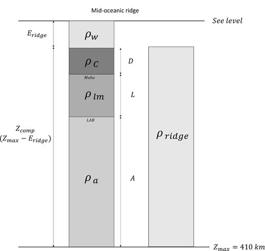
Reference column used in isostatic calculations. See text for details.

Open in new tab Download slide

From eqs (16), (17) and Fig. 2, the calibration constant can be expressed as

\begin{eqnarray*} L_{0} = Z_{max} - \dfrac{(\rho _{ridge}\times Z_{comp})+(E_{ridge} \times \rho _{w})}{\rho _{b}} . \end{eqnarray*}

(18)

For this work, we selected as the reference column a region located at long = 95°W and lat = 3.0°N on the Galapagos ridge. The average elevation, crustal thickness, crustal density and mantle density (all obtained from preliminary high-resolution inversions) at this location are all ‘standard’ MOR values of ∼−2800 m, 7 km, 2871 kg m⁻³ and 3409 kg m⁻³, respectively. Note that although the selection of the reference column is arbitrary in the context of local isostatic balance (any column where we can estimate average density and elevation with confidence would be acceptable), we chose our column in a region where most studies on large-scale global dynamic topography (e.g. Flament et al.2013) predict relatively small dynamic contributions.

4 TEMPERATURE, PRESSURE AND COMPOSITIONAL EFFECTS ON DENSITY

The average densities of the crust and sublithospheric mantle are assumed constant (but unknown) at each individual tesseroidal prism making up our global model. In the lithospheric mantle, however, density is assumed to be a function of pressure and temperature (and therefore of lithospheric thickness) according to

\begin{eqnarray*} \rho _{PT} = \rho _{0}[1-\alpha (T-T_{0})+\beta (P-P_{0})] , \end{eqnarray*}

(19)

where ρ₀ is the reference density at surface P-T conditions (i.e. T₀, P₀), α is the coefficient of thermal expansion and β the compressibility. Therefore, the average density of the lithospheric mantle at any specific location is

\begin{eqnarray*} \bar{\rho _{m}} = \frac{1}{(z_{LAB}-z_{M})}\int _{z_M}^{z_{LAB}} \rho _{PT} \,\, dz , \end{eqnarray*}

(20)

where z_M and z_LAB are the depths to the Moho and LAB, respectively. If we assume no radioactive heat production in the mantle (a standard first-order assumption in lithospheric modelling), the temperature profile in the mantle part of the lithosphere is linear and the process of obtaining the average density of the lithospheric mantle reduces to solving eq. (19) with T = |$\bar{T_{lm}}$| and P = |$\bar{P_{lm}}$| (i.e. the average temperature and pressure within the lithospheric mantle). In the following sections we explain how we obtain these average values (and how we implement compositional corrections to density in cratonic regions.

4.1 Geotherms and average lithospheric temperatures

If the geotherm is linear within the lithospheric mantle (i.e. steady-state with no heat sources), the average lithospheric mantle temperature |$\bar{T_{lm}}$| is simply

\begin{eqnarray*} \bar{T_{lm}} = \dfrac{T_{mh}+T_{LAB}}{2} , \end{eqnarray*}

(21)

where T_LAB is the temperature at the LAB and T_mh is the temperature at the Moho. The choice of defining the base of the lithosphere as an isotherm is common practice and related to the fact that the lithosphere is a thermal boundary layer and its mechanical properties are mainly controlled by temperature (cf. Burov 2011; Afonso et al.2016a). Most commonly used values are typically centred around 1300 °C, in agreement with numerous petrological, geophysical and geodynamic lines of evidence (e.g. Zlotnik et al.2008; Afonso et al.2008; Ballmer et al.2011; Burov 2011; Mckenzie et al.2005; McKenzie & Bickle 1988; O’Reilly & Griffin 2010; Shan et al.2014, Afonso et al.2016a,b; Green & Falloon 2015; among many others). We therefore assume T_LAB = 1300 °C in this study.

For continental crust, we obtain T_mh by solving the 1-D steady-state heat conduction equation with prescribed radiogenic heat productions and thermal conductivities for the crustal component. In doing so, and to better represent the actual curved crustal geotherm, we subdivide the crust into two layers (upper and lower crust) of equal thickness but possibly different radioactive heat production terms and thermal conductivities. Therefore, we write the final solution for T_mh as (e.g. Chapman 1986)

\begin{eqnarray*} T_{mh} = T_{s}+\frac{Q_{s}D}{2}\left(\frac{1}{K_{uc}}+\frac{1}{K_{lc}}\right)-\left(\frac{A_{uc}}{K_{uc}}+\frac{2A_{uc}+A_{lc}}{K_{lc}}\right)\frac{D^{2}}{8} , \end{eqnarray*}

(22)

where Q_s is surface heat flow, D is total crustal thickness, T_s (=10 °C) is surface temperature, K is thermal conductivity and A is radioactive heat production. Subscripts uc and lc refer to upper and lower crust, respectively, and adopted values are listed in Table 1.

Table 1.

Open in new tab

Parameters used in the calculation of lithospheric geotherms.

Symbol	Name	Value
α °C⁻¹)	Thermal expansion coef.	3.4 × 10⁻⁵
β (Pa⁻¹)	Compressibility coef.	1.1 × 10⁻⁶
K_uc\|$(\mathrm{W\, m^{-1}\, K}^{-1})$\|	Upper crust thermal conductivity	2.5
K_lc\|$(\mathrm{W\, m^{-1}\, K}^{-1})$\|	Lower crust thermal conductivity	2.2
K_m\|$(\mathrm{W\, m^{-1}\, K}^{-1})$\|	Mantle thermal conductivity	3.3
A_uc\|$\rm (\mu W\, m^{-3})$\|	Upper crust radioactive heat production	1.8
A_lc\|$\rm (\mu W\, m^{-3})$\|	Lower crust radioactive heat production	0.2
A_m\|$(\rm \mu W\, m^{-3})$\|	Mantle radioactive heat production	0

Symbol	Name	Value
α °C⁻¹)	Thermal expansion coef.	3.4 × 10⁻⁵
β (Pa⁻¹)	Compressibility coef.	1.1 × 10⁻⁶
K_uc\|$(\mathrm{W\, m^{-1}\, K}^{-1})$\|	Upper crust thermal conductivity	2.5
K_lc\|$(\mathrm{W\, m^{-1}\, K}^{-1})$\|	Lower crust thermal conductivity	2.2
K_m\|$(\mathrm{W\, m^{-1}\, K}^{-1})$\|	Mantle thermal conductivity	3.3
A_uc\|$\rm (\mu W\, m^{-3})$\|	Upper crust radioactive heat production	1.8
A_lc\|$\rm (\mu W\, m^{-3})$\|	Lower crust radioactive heat production	0.2
A_m\|$(\rm \mu W\, m^{-3})$\|	Mantle radioactive heat production	0

Table 1.

Open in new tab

Parameters used in the calculation of lithospheric geotherms.

Symbol	Name	Value
α °C⁻¹)	Thermal expansion coef.	3.4 × 10⁻⁵
β (Pa⁻¹)	Compressibility coef.	1.1 × 10⁻⁶
K_uc\|$(\mathrm{W\, m^{-1}\, K}^{-1})$\|	Upper crust thermal conductivity	2.5
K_lc\|$(\mathrm{W\, m^{-1}\, K}^{-1})$\|	Lower crust thermal conductivity	2.2
K_m\|$(\mathrm{W\, m^{-1}\, K}^{-1})$\|	Mantle thermal conductivity	3.3
A_uc\|$\rm (\mu W\, m^{-3})$\|	Upper crust radioactive heat production	1.8
A_lc\|$\rm (\mu W\, m^{-3})$\|	Lower crust radioactive heat production	0.2
A_m\|$(\rm \mu W\, m^{-3})$\|	Mantle radioactive heat production	0

Symbol	Name	Value
α °C⁻¹)	Thermal expansion coef.	3.4 × 10⁻⁵
β (Pa⁻¹)	Compressibility coef.	1.1 × 10⁻⁶
K_uc\|$(\mathrm{W\, m^{-1}\, K}^{-1})$\|	Upper crust thermal conductivity	2.5
K_lc\|$(\mathrm{W\, m^{-1}\, K}^{-1})$\|	Lower crust thermal conductivity	2.2
K_m\|$(\mathrm{W\, m^{-1}\, K}^{-1})$\|	Mantle thermal conductivity	3.3
A_uc\|$\rm (\mu W\, m^{-3})$\|	Upper crust radioactive heat production	1.8
A_lc\|$\rm (\mu W\, m^{-3})$\|	Lower crust radioactive heat production	0.2
A_m\|$(\rm \mu W\, m^{-3})$\|	Mantle radioactive heat production	0

In order to solve eq. (22) for any lithospheric thickness, we need the corresponding Q_s in continents. The latter can be obtained or approximated in a number of ways (e.g. from a database of observations, from a thermal model, etc). Here we prefer to estimate Q_s from the solution to the 1D steady-state heat conduction equation of a three-layer lithosphere rather than using global databases, which are extremely sparse and would require treating thermal parameters in the crust (e.g. A_uc, A_lc) as additional free parameters of the model. We note, however, that our predicted Q_s values are comparable to those in many global databases (Fig. S4), so our final model can also be considered to the first order compatible with most compilations and estimates of global surface heat flow data (e.g. Shapiro & Ritzwoller 2004; Davies & Davies 2010; Goutorbe et al.2011).

The solution to the steady-state conduction equation for a three-layer (upper crust, lower crust, lithospheric mantle) lithosphere can be written as (e.g. Afonso & Ranalli 2004)

\begin{eqnarray*} Q_{s} = \dfrac{T_{LAB}-T_{s}+\left(\frac{A_{uc}}{K_{uc}}+\frac{2A_{uc}+A_{lc}}{K_{lc}}\right)\frac{D^{2}}{8}+\left(\dfrac{A_{uc}+A_{lc}}{2K_{m}}\right)D.L}{\frac{D}{2}\left(\frac{1}{K_{uc}}+\frac{1}{K_{lc}}\right)+\dfrac{L}{K_{m}}} , \end{eqnarray*}

(23)

where L is the thickness of the lithospheric mantle and K_m its thermal conductivity. In deriving eq. (23), we assumed A_m = 0 and made use of the relation

\begin{eqnarray*} Q_{m} = Q_{s}-\bigg(\dfrac{A_{u}+A_{l}}{2}\bigg).D . \end{eqnarray*}

(24)

In the oceanic domain, we compute the lithospheric thermal structure and corresponding T_mh following the plate model of Grose & Afonso (2013) with crustal age from Müller et al. (2008).

4.2 Pressure

At each iteration of our algorithm, the average pressure within the lithospheric mantle |$\bar{P_{lm}}$| is obtained from the lithostatic formula

\begin{eqnarray*} \bar{P_{lm}} = \bigg(\rho _{c}.D+\rho _{0}.\dfrac{L}{2}\bigg).g . \end{eqnarray*}

(25)

Given the goals of our study, we choose not to implement an additional iterative scheme for the pressure-density coupling (e.g. Afonso et al.2008), but instead we update the values of ρ_c, D and L at each iteration of the algorithm with those obtained at the previous iteration (see Section 6). This simplification affects our results to the second order only. Eq. (25) also ignores dynamic pressure gradients arising from sublithospheric convection (not modelled here), in agreement with our local isostasy assumption (Section 3.2). This means that dynamic contributions to topography will be ‘lumped’ into the density anomalies of the model and therefore they should represent upper bounds. This needs to be taken into consideration when interpreting the inversion’s results (see Section 8.1). However, the actual effect on average mantle density values is expected to be small given the fact that elevation changes of the order of 500–600 m can be compensated by only minor changes in Moho depth and/or average mantle density (i.e. a small change in the average density of a mantle column has a major effect on the predicted topography; Lachenbruch & Morgan 1990; Hasterok & Chapman 2007; Molnar et al.2015; Afonso et al.2016b).

4.3 Compositional correction in cratonic regions

It is generally accepted that the lithospheric mantle beneath cratonic regions is more depleted in heavy elements (e.g. CaO, Al₂O₃ and FeO) than the average lithospheric mantle (cf. Griffin et al.2003, 2009; Lee et al.2011), particularly at the shallowest levels of the lithospheric keels. This idea is not only supported by what it is directly observed in mantle samples (Griffin et al.2009) but also by geophysical and geodynamic arguments (e.g. Jordan 1988; Forte & Perry 2000; Carlson et al.2005; Afonso et al.2008; Cammarano et al.2011; Khan et al.2011; Wang et al.2015). Based on these studies, we subdivide the lithospheric mantle beneath cratonic keels into two layers. The top layer is given a maximum depth of 175 km and is assumed to be significantly depleted with respect to the average mantle. The second layer is assumed to be more fertile (still slightly more depleted than sublithospheric mantle) and extends from the bottom of the top layer to the LAB. In practice, these assumptions are implemented via the ρ₀ term (reference density at surface conditions) in eq. (19), as this term is affected the most by compositional changes (the effects on thermal expansion and compressibility are much smaller). Following the study of Lee (2003), we choose |$\rho _{0} = 3325 \, \mathrm{kg\, m}^{-2}$| for the top layer (‘dunitic/harzburgitic’ rocks), |$\rho _{0} = 3355 \, \mathrm{kg\, m}^{-2}$| for the bottom cratonic layer and |$\rho _{0} = 3360 \, \mathrm{kg\, m}^{-2}$| for all other mantle domains. The lateral extension of cratonic domains in our model correspond that of early Proterozoic/Archean age crust in the model CRUST1.0 (Laske et al.2013).

5 MODEL DISCRETIZATION AND MAIN FREE PARAMETERS

The lateral discretization of our model corresponds to a 2° × 2° regular grid (see Fig. 3). Due to the convergence of meridians at the poles, the original 2° × 2° tesseroids become too irregular at latitudes >80° to be accurately represented by a rectangular prism. We therefore subdivide these tesseroids along latitude to guarantee an accurate solution; results from the inversion, however, are reported for the original 2° × 2° grid. We acknowledge that more efficient meshing/discretization approaches are possible (e.g. equal-area grid) and we are currently exploring these possibilities.

Figure 3.

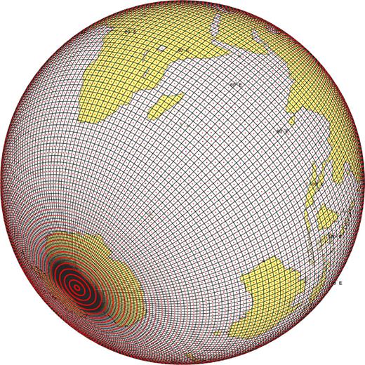
Horizontal discretization as a 2° × 2° fixed grid. The red points are the surface centroids of the tesseroids and indicate observation/calculation points.

Open in new tab Download slide

Along the vertical direction, each tesseroidal column extends down to 410 km and is subdivided into four segments of variable thickness: sea water (if present), crust, lithospheric mantle and sublithospheric upper mantle. Each of these segments are in turn subdivided into a variable number of smaller tesseroidal volumes (depending on the thickness of the segment) to guarantee that the prism approximation remains valid for the entire column.

According to the above discretization, our main model parameters are (i) crustal thickness, (ii) depth to the LAB, (iii) average density of the crust and (iv) average density of the sublithospheric upper mantle (from the LAB down to 410 km depth) for every column in our model (see Fig. 4). Note that the complete temperature and density structures of the entire lithosphere are by-products of the inversion and thus considered outputs of the model (see e.g. Fig. S5).

$Schematic of the vertical discretization and main parameteres. Encircled variables (i.e. Moho, LAB, $\overline{\rho }_{a}$ and $\overline{\rho }_{c}$) are the main free parameters inverted for (i.e. elements of vector m). The lithospheric geotherm and $\overline{\rho }_{lm}$ are by-products of the inversion and thus outputs of the model.$

Figure 4.

Schematic of the vertical discretization and main parameteres. Encircled variables (i.e. Moho, LAB, |$\overline{\rho }_{a}$| and |$\overline{\rho }_{c}$|⁠) are the main free parameters inverted for (i.e. elements of vector m). The lithospheric geotherm and |$\overline{\rho }_{lm}$| are by-products of the inversion and thus outputs of the model.

Open in new tab Download slide

6 INVERSION STRATEGY

6.1 General problem formulation

The general formulation followed here is similar to that described in Motavalli-Anbaran et al. (2013). All input data are projected onto the regular 2° × 2° grid. Therefore, the combined data vector has the following form and dimension

\begin{eqnarray*} \mathbf {d_{obs}} &=& [H_{_{i}},\Delta g_{_{i}},\Delta g_{_{i}}^{xx},\Delta g_{_{i}}^{yy},\Delta g_{_{i}}^{zz},\Delta N_{_{i}}]^{T} \, \, \, \, \, \, \, \, \, \, i = 1,16200 \nonumber \\ &=& [d_{_{1}},...,d_{N}]^{T}\, \, \, \, \, \, \, \, \, \, N = 1,97200 \end{eqnarray*}

(26)

where H, Δg and ΔN are the vectors containing elevation, free-air gravity anomalies and geoid heights, respectively; Δg^xx, Δg^yy and Δg^zz are the data vectors containing the diagonal terms of the gravity gradient tensor.

The model parameters are stored in the following combined vector

\begin{eqnarray*} \mathbf {m} &=& [\rho ^{c}_{j},\rho ^{a} _{_{j}},Z^{c}_{_{j}},Z^{l}_{_{j}}]^{T}\, \, \, \, \, \, \, \, \, j = 1,16200\nonumber \\ &=& [m_{_{1}},...,m_{M}]^{T}\, \, \, \, \, \, \, \, \, M = 1,64800 , \end{eqnarray*}

(27)

where ρ^c, ρ^a, Z^c and Z^l are vectors containing the values of crustal density, sublithospheric mantle average density, crustal thickness and LAB depth.

The basic requirement of all inverse problems is that there is a function |${\bf g}(\mathbf {m})$| that maps a vector of model parameters |$\mathbf {m}$| into a data space |$\mathbf {d}$|⁠. This mapping is known as the forward problem and is denoted by

\begin{eqnarray*} {\bf d}^{pred} = {\bf g}({\bf m}) , \end{eqnarray*}

(28)

where d^pred is the predicted data vector. When |${\bf g}(\mathbf {m})$| is a nonlinear function, as in our case, a typical approach is to locally linearize the problem in the vicinity of trial solutions |$\mathbf {m^{^{\prime }}}$| and solve local linear problems in an iterative manner until a predefined ‘global error’ is optimally minimized (Tarantola 2005; Menke 2012). By global error we mean certain function that quantifies the distance between the vectors of observed data d^obs (eq. 26) and predicted data d^pred (eq. 28). This function is commonly referred to as the misfit function, the objective function, or simply the error function. Assuming Gaussian statistics for the errors (a standard, yet no always justified, assumption) and the availability of a reference or a priori vector of model parameters |$\mathbf {m_o}$|⁠, we can define the misfit function as

\begin{eqnarray*} 2 \, \varPhi (\mathbf {m}) = [{\bf g}(\mathbf {m})-\mathbf {d}^{obs}]^{T}{\bf C}_{D}^{-1}[{\bf g}(\mathbf {m})-\mathbf {d}^{obs}]+[{\bf m}-{\bf m}_{0}]^{T}{\bf C}_{M}^{-1}[{\bf m}-{\bf m}_{0}] , \end{eqnarray*}

(29)

where C_D is the data covariance matrix and C_M is the model covariance matrix. Note that we do not include a damping factor in the second term of the right-hand side, and therefore prior information on the model is combined with data constraints in a way more akin to a Bayesian approach (cf. Tarantola 2005; Rawlinson et al.2014). In this sense, including C_M in eq. (29) not only allows us to make use of additional constraints independent from the observations (e.g. prior estimates of LAB depths) but also stabilizes the solution of the (ill-posed) inverse problem by acting as a regularization term. Both C_D and C_M are assumed here to be diagonal. In practice, while we may have a good idea of the diagonal terms in C_M, we rarely know the general structure of C_D. At the same time, its elements are usually smaller than the errors associated with the forward problem. Therefore, C_D is mainly used to define the relative contribution of each data set to the global misfit function (i.e. as a weighting matrix; Menke 2012). For instance, in this study, our main interest is to obtain models that fit well geoid heights, free-air anomalies and gravity gradients while being simultaneously consistent with, but not strictly controlled by, topography data (since the assumption of local isostatic equilibrium may not be a good approximation everywhere). Therefore, the elements of C_D corresponding to elevation data will have a smaller relative weight than those corresponding to the other datasets. With this in mind, we performed numerous tests to obtain the appropriate elements of C_D for each data set that would result in a (relative) satisfactory fit of all observables (see Table 2).

Table 2.

Open in new tab

Initial standard deviations used in the covariance matrices |$\mathbf {C_D}$| and |$\mathbf {C_M}$|⁠.

Observations	Δg	ΔN	H	Δg^xx	Δg^yy	Δg^zz
σ^d (Data standard deviation)	5 (mGal)	0.5 (m)	200 (m)	0.08 (E)	0.08 (E)	0.08 (E)
Model parameters			ρ^c	ρ^a	Z^c	Z^l
σ^p (Parameter standard deviation)			5 \|$(\mathrm{kg\, m}^{-3})$\|	5 \|$(\mathrm{kg\, m}^{-3})$\|	500 (m)	1000 (m)

Observations	Δg	ΔN	H	Δg^xx	Δg^yy	Δg^zz
σ^d (Data standard deviation)	5 (mGal)	0.5 (m)	200 (m)	0.08 (E)	0.08 (E)	0.08 (E)
Model parameters			ρ^c	ρ^a	Z^c	Z^l
σ^p (Parameter standard deviation)			5 \|$(\mathrm{kg\, m}^{-3})$\|	5 \|$(\mathrm{kg\, m}^{-3})$\|	500 (m)	1000 (m)

Table 2.

Open in new tab

Initial standard deviations used in the covariance matrices |$\mathbf {C_D}$| and |$\mathbf {C_M}$|⁠.

Observations	Δg	ΔN	H	Δg^xx	Δg^yy	Δg^zz
σ^d (Data standard deviation)	5 (mGal)	0.5 (m)	200 (m)	0.08 (E)	0.08 (E)	0.08 (E)
Model parameters			ρ^c	ρ^a	Z^c	Z^l
σ^p (Parameter standard deviation)			5 \|$(\mathrm{kg\, m}^{-3})$\|	5 \|$(\mathrm{kg\, m}^{-3})$\|	500 (m)	1000 (m)

Observations	Δg	ΔN	H	Δg^xx	Δg^yy	Δg^zz
σ^d (Data standard deviation)	5 (mGal)	0.5 (m)	200 (m)	0.08 (E)	0.08 (E)	0.08 (E)
Model parameters			ρ^c	ρ^a	Z^c	Z^l
σ^p (Parameter standard deviation)			5 \|$(\mathrm{kg\, m}^{-3})$\|	5 \|$(\mathrm{kg\, m}^{-3})$\|	500 (m)	1000 (m)

6.2 Inversion algorithm

A typical approach for linearizing |$\varPhi (\mathbf {m})$| is based on a Taylor series expansion about the vector of known initial parameter |$\mathbf {m}_{k}$|

\begin{eqnarray*} \varPhi ({\bf m}_{k}+\Delta {\bf m})\simeq \varPhi (\mathbf {m}_{k})+ \boldsymbol{\gamma }^{T}_{k}\Delta {\bf m}+\dfrac{1}{2}\Delta {\bf m}^{T}{\bf H}_{k} \Delta {\bf m}+... , \end{eqnarray*}

(30)

where the matrices H_k and |$\boldsymbol{\gamma }_{k}$| contain the second-order (Hessian matrix) and first-order partial derivatives of the misfit function at m_k, respectively. The problem is thus to find Δm that makes the global error smaller in a L2-norm sense by updating the parameter vector from m_k to the stationary point

\begin{eqnarray*} {\bf m}_{k+1} = {\bf m}_{k}+\Delta {\bf m} . \end{eqnarray*}

(31)

The solution to the inverse problem is obtained by setting the gradient of eq. (30) with respect to Δm to zero, which gives the following (quasi-Newton) iterative scheme (Tarantola 2005)

\begin{eqnarray*} {\bf m}_{k+1}-{\bf m}_{k} = \biggr ( {\bf G}^{T}_{k} {\bf C}^{-1}_{D}{\bf G}_{k}+ {\bf C}^{-1}_{M}\biggr )^{-1} \biggr ({\bf G}^{T} {\bf C}^{-1}_{D} ({\bf d}^{obs}-{\bf g}({\bf m}_{k}))+{\bf C}^{-1}_{M}({\bf m}_{k}-{\bf m}_{0}) \biggr ) , \end{eqnarray*}

(32)

where k denotes the iteration number and G_k is the Jacobian matrix containing the partial derivatives of g(.) with respect to m (⁠|${}[\dfrac{\partial d_{i}}{\partial m_{j}}]_{k}$|⁠). In deriving eq. (32) we have made use of the following standard approximation of the Hessian (Tarantola 2005)

\begin{eqnarray*} {\bf H}_{k} \sim {\bf G}^{T}_{k} {\bf C}^{-1}_{D}{\bf G}_{k} + {\bf C}^{-1}_{M} . \end{eqnarray*}

(33)

The entries of the Jacobian matrix G_k corresponding to the densities in the crust and sublithospheric mantle are linear and thus readily calculated as the effect of body j at point i divided by the actual density of the body. In contrast, the elements associated with crustal thickness and LAB depth are non-linear and therefore calculated numerically with a finite difference scheme.

After the first iteration, in which eq. (32) is solved with m₀ from the initial model, we update the values in m₀ with those obtained at the previous iteration. In this way m is not necessarily forced to remain close to the initial model (unless dictated by the prior) and the last term in eq. (32) vanishes. For iterations other than the first one, eq. (32) can therefore be rewritten as

\begin{eqnarray*} {\bf m}_{k+1}-{\bf m}_{k} = {\bf K}\times ({\bf d}^{obs}-{\bf g}({\bf m}_{k})), \end{eqnarray*}

(34)

where K is the kernel matrix defined as

\begin{eqnarray*} {\bf K} = \biggr ( {\bf G}^{T}_{k} {\bf C}^{-1}_{D}{\bf G}_{k}+ {\bf C}^{-1}_{M}\biggr )^{-1} {\bf G}^{T} {\bf C}^{-1}_{D} . \end{eqnarray*}

(35)

The general parallelized procedure used to solve eqs (32)–(35) is summarized in Fig. 5 and described in Appendix A.

Figure 5.

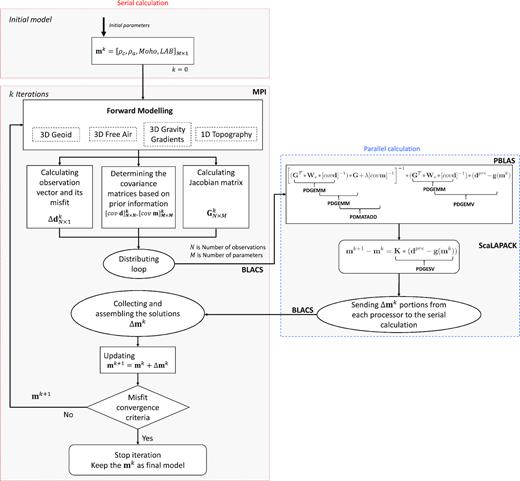
Flowchart of the inversion scheme used in this work. Note that the temperature, pressure, and compositional corrections described in Section 4 are included in the box ‘1-D Topography’. See also Appendix A.

Open in new tab Download slide

7 SYNTHETIC TESTS AND SENSITIVITY ANALYSIS

7.1 Global synthetic tests

The synthetic model used here is a full 3-D, 1° × 1° spherical model of the Earth with an uneven distribution of parameters (i.e. crustal density, crustal thickness, LAB depth, asthenospheric density; Table 3) with sharp boundaries and varying amplitudes (Fig. 6, first column). The initial topography/bathymetry is isostatically compensated everywhere as follows: 90 |$\hbox{ per cent}$| by the crust and 10 |$\hbox{ per cent}$| by the lithospheric mantle. To obtain the synthetic data we solved all forward problems and added uncorrelated random Gaussian noise with zero mean and standard deviation of 10|$\hbox{ per cent}$|⁠. Free-air and geoid anomalies are computed/provided at the Earth’s surface, whereas gravity gradients are computed at 250 km above the Earth’s surface (average orbit height of GOCE satellite). After these synthetic data sets are computed, we interpolate them to the 2° × 2° grid used in the inversion. The standard deviations associated with the synthetic data σ^d (used to compute the variances in C_D) are the same in all tests and equal to |$\sigma ^d_{FA}$| = 5 mGal, |$\sigma ^d_{G}$| = 0.5 m, |$\sigma ^d_{E}$| = 100 m, and |$\sigma ^d_{gg}$| = 0.08 E|$\ddot{o}$| tvos, for free-air anomalies, geoid height, elevation and gravity gradients, respectively.

Figure 6.

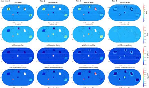
Results from synthetic tests using different initial models in the inversion. The true model is shown in the leftmost column. Test 1 uses an initial model that is close to the true model. Test 2 uses an initial model that is farther away from the true model, yet still within reasonable limits. In Test 3, the initial model is a spherically symmetric model (i.e. flat surfaces) with no information of any anomaly or discontinuity; this is an unrealistic worse-case scenario in practical applications.

Open in new tab Download slide

Table 3.

Open in new tab

Parameters used in the synthetic model. The region numbers correspond to those in Fig. 6.

Region	Elev. (m)	Crust den. (⁠\|$\, \mathrm{kg\, m}^{-3}$\|⁠)	Asthe. den. (⁠\|$\, \mathrm{kg\, m}^{-3}$\|⁠)	Moho (m)	LAB (m)
1	3000	2750	3395	43547	132331
2	2500	2770	3450	53820	217215
3	-3000	3000	3390	20805	179361
4	3500	2770	3385	45798	115514
5	4500	2740	3470	64263	234235
6	1000	2790	3410	38251	166585

Region	Elev. (m)	Crust den. (⁠\|$\, \mathrm{kg\, m}^{-3}$\|⁠)	Asthe. den. (⁠\|$\, \mathrm{kg\, m}^{-3}$\|⁠)	Moho (m)	LAB (m)
1	3000	2750	3395	43547	132331
2	2500	2770	3450	53820	217215
3	-3000	3000	3390	20805	179361
4	3500	2770	3385	45798	115514
5	4500	2740	3470	64263	234235
6	1000	2790	3410	38251	166585

Table 3.

Open in new tab

Parameters used in the synthetic model. The region numbers correspond to those in Fig. 6.

Region	Elev. (m)	Crust den. (⁠\|$\, \mathrm{kg\, m}^{-3}$\|⁠)	Asthe. den. (⁠\|$\, \mathrm{kg\, m}^{-3}$\|⁠)	Moho (m)	LAB (m)
1	3000	2750	3395	43547	132331
2	2500	2770	3450	53820	217215
3	-3000	3000	3390	20805	179361
4	3500	2770	3385	45798	115514
5	4500	2740	3470	64263	234235
6	1000	2790	3410	38251	166585

Region	Elev. (m)	Crust den. (⁠\|$\, \mathrm{kg\, m}^{-3}$\|⁠)	Asthe. den. (⁠\|$\, \mathrm{kg\, m}^{-3}$\|⁠)	Moho (m)	LAB (m)
1	3000	2750	3395	43547	132331
2	2500	2770	3450	53820	217215
3	-3000	3000	3390	20805	179361
4	3500	2770	3385	45798	115514
5	4500	2740	3470	64263	234235
6	1000	2790	3410	38251	166585

For the first test, we start the inversion with an initial model that is close to the true model (see Tables 3 and 4). The parameters retrieved by the inversion are shown in Fig. 6 (second column) and Table 4. In this case, the algorithm recovers the true parameters almost exactly in a few iterations; all of the model parameters are drawn closer to the true values than in the initial model, even when the original data is noisy.

Table 4.

Open in new tab

Initial and retrieved values for the main model parameters for all tests.

Inversion result					Initial model
Region	Crust den. (⁠\|$\, \mathrm{kg\, m}^{-3}$\|⁠)	Asthe. den. (⁠\|$\, \mathrm{kg\, m}^{-3}$\|⁠)	Moho (m)	LAB (m)	Crust den. (⁠\|$\, \mathrm{kg\, m}^{-3}$\|⁠)	Asthe. den. (⁠\|$\, \mathrm{kg\, m}^{-3}$\|⁠)	Moho (m)	LAB (m)
Test 1
1	2748	3399	43827	133901	2760	3385	41547	136331
2	2774	3451	53931	218919	2780	3440	51820	221215
3	2994	3394	20554	180211	3010	3380	18805	183361
4	2773	3386	45993	116514	2780	3375	43798	119514
5	2739	3468	64913	233914	2750	3460	62263	238235
6	2788	3409	38911	167815	2800	3400	36251	170585
Test 2
1	2753	3387	38546	144821	2760	3375	38547	142331
2	2778	3443	48820	224022	2780	3430	46820	227215
3	2993	3386	19942	183302	3010	3370	15805	189361
4	2776	3383	43863	116413	2780	3365	40798	125514
5	2743	3462	59943	235213	2750	3450	59263	248235
6	2795	3398	36815	169894	2800	3990	33251	176585
Test 3
1	2774	3387	31586	145525	2780	3400	30000	145000
2	2755	3389	32584	144828	2780	3400	30000	145000
3	2823	3432	24987	139542	2780	3400	30000	145000
4	2752	3389	31582	146121	2780	3400	30000	145000
5	2749	3392	34374	146951	2780	3400	30000	145000
6	2784	3394	31025	144980	2780	3400	30000	145000

Inversion result					Initial model
Region	Crust den. (⁠\|$\, \mathrm{kg\, m}^{-3}$\|⁠)	Asthe. den. (⁠\|$\, \mathrm{kg\, m}^{-3}$\|⁠)	Moho (m)	LAB (m)	Crust den. (⁠\|$\, \mathrm{kg\, m}^{-3}$\|⁠)	Asthe. den. (⁠\|$\, \mathrm{kg\, m}^{-3}$\|⁠)	Moho (m)	LAB (m)
Test 1
1	2748	3399	43827	133901	2760	3385	41547	136331
2	2774	3451	53931	218919	2780	3440	51820	221215
3	2994	3394	20554	180211	3010	3380	18805	183361
4	2773	3386	45993	116514	2780	3375	43798	119514
5	2739	3468	64913	233914	2750	3460	62263	238235
6	2788	3409	38911	167815	2800	3400	36251	170585
Test 2
1	2753	3387	38546	144821	2760	3375	38547	142331
2	2778	3443	48820	224022	2780	3430	46820	227215
3	2993	3386	19942	183302	3010	3370	15805	189361
4	2776	3383	43863	116413	2780	3365	40798	125514
5	2743	3462	59943	235213	2750	3450	59263	248235
6	2795	3398	36815	169894	2800	3990	33251	176585
Test 3
1	2774	3387	31586	145525	2780	3400	30000	145000
2	2755	3389	32584	144828	2780	3400	30000	145000
3	2823	3432	24987	139542	2780	3400	30000	145000
4	2752	3389	31582	146121	2780	3400	30000	145000
5	2749	3392	34374	146951	2780	3400	30000	145000
6	2784	3394	31025	144980	2780	3400	30000	145000

Table 4.

Open in new tab

Initial and retrieved values for the main model parameters for all tests.

Inversion result					Initial model
Region	Crust den. (⁠\|$\, \mathrm{kg\, m}^{-3}$\|⁠)	Asthe. den. (⁠\|$\, \mathrm{kg\, m}^{-3}$\|⁠)	Moho (m)	LAB (m)	Crust den. (⁠\|$\, \mathrm{kg\, m}^{-3}$\|⁠)	Asthe. den. (⁠\|$\, \mathrm{kg\, m}^{-3}$\|⁠)	Moho (m)	LAB (m)
Test 1
1	2748	3399	43827	133901	2760	3385	41547	136331
2	2774	3451	53931	218919	2780	3440	51820	221215
3	2994	3394	20554	180211	3010	3380	18805	183361
4	2773	3386	45993	116514	2780	3375	43798	119514
5	2739	3468	64913	233914	2750	3460	62263	238235
6	2788	3409	38911	167815	2800	3400	36251	170585
Test 2
1	2753	3387	38546	144821	2760	3375	38547	142331
2	2778	3443	48820	224022	2780	3430	46820	227215
3	2993	3386	19942	183302	3010	3370	15805	189361
4	2776	3383	43863	116413	2780	3365	40798	125514
5	2743	3462	59943	235213	2750	3450	59263	248235
6	2795	3398	36815	169894	2800	3990	33251	176585
Test 3
1	2774	3387	31586	145525	2780	3400	30000	145000
2	2755	3389	32584	144828	2780	3400	30000	145000
3	2823	3432	24987	139542	2780	3400	30000	145000
4	2752	3389	31582	146121	2780	3400	30000	145000
5	2749	3392	34374	146951	2780	3400	30000	145000
6	2784	3394	31025	144980	2780	3400	30000	145000

Inversion result					Initial model
Region	Crust den. (⁠\|$\, \mathrm{kg\, m}^{-3}$\|⁠)	Asthe. den. (⁠\|$\, \mathrm{kg\, m}^{-3}$\|⁠)	Moho (m)	LAB (m)	Crust den. (⁠\|$\, \mathrm{kg\, m}^{-3}$\|⁠)	Asthe. den. (⁠\|$\, \mathrm{kg\, m}^{-3}$\|⁠)	Moho (m)	LAB (m)
Test 1
1	2748	3399	43827	133901	2760	3385	41547	136331
2	2774	3451	53931	218919	2780	3440	51820	221215
3	2994	3394	20554	180211	3010	3380	18805	183361
4	2773	3386	45993	116514	2780	3375	43798	119514
5	2739	3468	64913	233914	2750	3460	62263	238235
6	2788	3409	38911	167815	2800	3400	36251	170585
Test 2
1	2753	3387	38546	144821	2760	3375	38547	142331
2	2778	3443	48820	224022	2780	3430	46820	227215
3	2993	3386	19942	183302	3010	3370	15805	189361
4	2776	3383	43863	116413	2780	3365	40798	125514
5	2743	3462	59943	235213	2750	3450	59263	248235
6	2795	3398	36815	169894	2800	3990	33251	176585
Test 3
1	2774	3387	31586	145525	2780	3400	30000	145000
2	2755	3389	32584	144828	2780	3400	30000	145000
3	2823	3432	24987	139542	2780	3400	30000	145000
4	2752	3389	31582	146121	2780	3400	30000	145000
5	2749	3392	34374	146951	2780	3400	30000	145000
6	2784	3394	31025	144980	2780	3400	30000	145000

The results for the second test are shown in Fig. 6 (third column). Here, the starting model is farther from the true model, yet within reasonable/realistic bounds (Tables 3 and 4). The final model still represents a clear improvement over the starting model; all the parameters are well recovered and closer to the true model than in the initial model. Region 1 is an interesting exception, where the inversion has not been able to recover the true LAB depth, although it did produce acceptable results for all other parameters. This case illustrates an unavoidable limitation of linearized algorithms such as the one used in this work, which are not suited to recognize two or more possible models with identical misfit characteristics. In the present case, our initial (deliberate) combination of model parameters (thicker LAB and thinner crust) in region 1 balance each other to produce similar observables to those predicted by the true model (thus the inversion still gives an acceptable fit to observations) and therefore the inversion favours a solution closer to the (wrong) starting model. Stochastic or probabilistic inversion algorithms are less sensitive to this problem, but significantly more computationally expensive, which has rendered them impractical for this work. The implementation of such non-linear, matrix-free algorithms for global inversions is currently under development by the authors.

In the third test (Fig. 6, fourth column), we start the inversion with a spherically symmetric model, therefore containing no information on any type of anomaly. This case is purely illustrative as it represents a worst-case scenario, unlikely to occur in any real application. Results in Fig. 6 (fourth column) show that, while the inversion improved the density values of the initial model in some regions, overall it could not produce acceptable results, especially for Moho and LAB depths.

7.2 Removing the effects of unmodelled density anomalies in the input data sets

Before presenting the final model and main results, we briefly discuss the issue of removing signals in the input data sets that arise from unmodelled (deep) density anomalies. As mentioned before, it is customary to filter out long wavelengths from the total geoid to minimize the effects of deep (depths >410 km) density anomalies (e.g. Ricard et al.1984; Chase 1985; Bowin 1983; Marks et al.1991; Bowin 2000; Featherstone 1997; Chase et al.2002; Coblentz et al.2011; Fullea et al.2015; Afonso et al.2016c). Many studies have shown theoretically and empirically that under some reasonable assumptions, removing spherical harmonics lower than 8–15 from the total geoid leave a signal controlled mostly to density anomalies within the first 300–410 km (e.g. Crough & Jurdy 1980; Hager 1984; Chase 1985; Hager & Richards 1989; Bowin 1983, 2000; Doin et al.1996). Since here we jointly invert multiple fields, we filter all of them to the same degree for consistency (except for topography given its local nature at the scale of interest). However, in principle, not all fields have the same sensitivity to deeper/shallow anomalies, making the issue of finding an optimal filter more problematic than in the case of working with only one field. Moreover, all masses inside the Earth contribute to all degrees (albeit differentially) in a spherical expansion and therefore wavelength filtering can never be completely satisfactory.

We address this issue with a pragmatic two-fold approach. First, we run synthetic tests to gauge the contribution of density anomalies of different sizes and at different depths to the total signal and to each harmonic degree for all fields used in this work. We performed these tests for both localized anomalies and for whole-Earth mantle models (see Supporting Information). Secondly, informed by these synthetic tests, we performed multiple inversions of the real data sets filtered at different degrees and analyse the fitting statistics. The guiding principle here is that those fields that either retain signals/contributions from unmodelled deeper sources or do not include contributions from significant anomalies within the modelled region, will tend to produce poorer joint fits than those where most of the causative density heterogeneity in all fields is properly accounted for by the model. We tested five cases in which we filtered the data to leave degrees/orders ≥6, 8, 10, 12 and 14 in the spherical harmonic expansions of the fields. Both approaches converged to the same conclusion, namely that filtering up to degree and order ∼10 is optimal in terms of both explicative power (e.g. quality of joint fit) and spectral power (see Figs S1–S3).

It can be shown, however, that the effect of density anomalies located between 410 and 1000 km depth is non-negligible on a filtered geoid up to degree and order ∼10 in many parts of the planet (Fig. S3). Not accounting for this effect would introduce undesired biases into the model by forcing incorrect density values to compensate for unmodelled deeper anomalies. We therefore decided to explicitly account for density anomalies at depths >410 km (by computing their contribution using a global density model; Panning & Romanowicz 2006) and remove their effect from the observed filtered fields. The above analyses and data processing approach give us confidence that our results presented in the following section will not be contaminated by unmodelled density anomalies to any major extent.

8 RESULTS

8.1 Fits to data

Fig. 7 shows the observables used in the inversion and those predicted by the final model after 18 iterations of our algorithm. The quality of the joint fit is satisfactory for all fields and all the main patterns in the data sets are explained to a high degree of precision. The summary statistics in Tables 5 and 6 clearly show that our final model not only displays acceptable joint misfits, but also represents a significant improvement over the initial/starting model. Interestingly, the long-wavelength misfit in elevation follows closely the pattern predicted by global models of dynamic topography (see Flament et al.2013, for a recent review), except perhaps in southeast Asia and northern Oceania. In addition, the systematic misfit along MORs seems to be related to (at least) two limitations in the model parametrization: (1) the model does not account for the shallow low density structure beneath MORs (i.e. the so-called melting region) and (2) a single sublithospheric column of uniform density beneath MORs is required to simultaneously fit all data sets (those sensitive to shallow anomalies as well as those sensitive to deeper anomalies) and therefore a biased compromise solution is required. Shallow dynamic effects are also a possible factor. Considering all of the above, we decided not to peruse better fits to elevation, as these misfits likely contain dynamic components not included in our inversion and/or biases due to the simple parametrization adopted for the mantle.

Figure 7.

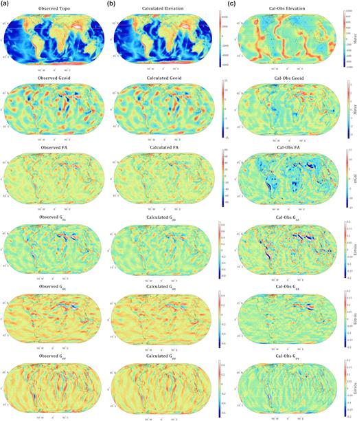
(a) Observed data used in the inversion. (b) Predicted data by the final model. (c) Data residuals (predicted - observed) of the final model. All fields have been interpolated to a 1° × 1° for illustration purposes.

Open in new tab Download slide

Table 5.

Open in new tab

RMS of data misfits associated with LithoRef18.

Iteration	Elev. (m)	Geoid (m)	Free air (mGal)	Grad.xx (Eotvos)	Grad.yy (Eotvos)	Grad.zz (Eotvos)
Initial model	2.1255e+03	561.1871	269.1086	1.2269	1.3436	2.2365
1	654.3586	3.3718	7.4776	0.0492	0.0550	0.0800
2	552.0082	1.5816	4.6181	0.0403	0.0403	0.0583
\|$\colon$\|	\|$\colon$\|	\|$\colon$\|	\|$\colon$\|	\|$\colon$\|	\|$\colon$\|	\|$\colon$\|
18	220.8516	0.6965	3.3833	0.0353	0.0364	0.0494

Iteration	Elev. (m)	Geoid (m)	Free air (mGal)	Grad.xx (Eotvos)	Grad.yy (Eotvos)	Grad.zz (Eotvos)
Initial model	2.1255e+03	561.1871	269.1086	1.2269	1.3436	2.2365
1	654.3586	3.3718	7.4776	0.0492	0.0550	0.0800
2	552.0082	1.5816	4.6181	0.0403	0.0403	0.0583
\|$\colon$\|	\|$\colon$\|	\|$\colon$\|	\|$\colon$\|	\|$\colon$\|	\|$\colon$\|	\|$\colon$\|
18	220.8516	0.6965	3.3833	0.0353	0.0364	0.0494

Table 5.

Open in new tab

RMS of data misfits associated with LithoRef18.

Iteration	Elev. (m)	Geoid (m)	Free air (mGal)	Grad.xx (Eotvos)	Grad.yy (Eotvos)	Grad.zz (Eotvos)
Initial model	2.1255e+03	561.1871	269.1086	1.2269	1.3436	2.2365
1	654.3586	3.3718	7.4776	0.0492	0.0550	0.0800
2	552.0082	1.5816	4.6181	0.0403	0.0403	0.0583
\|$\colon$\|	\|$\colon$\|	\|$\colon$\|	\|$\colon$\|	\|$\colon$\|	\|$\colon$\|	\|$\colon$\|
18	220.8516	0.6965	3.3833	0.0353	0.0364	0.0494

Iteration	Elev. (m)	Geoid (m)	Free air (mGal)	Grad.xx (Eotvos)	Grad.yy (Eotvos)	Grad.zz (Eotvos)
Initial model	2.1255e+03	561.1871	269.1086	1.2269	1.3436	2.2365
1	654.3586	3.3718	7.4776	0.0492	0.0550	0.0800
2	552.0082	1.5816	4.6181	0.0403	0.0403	0.0583
\|$\colon$\|	\|$\colon$\|	\|$\colon$\|	\|$\colon$\|	\|$\colon$\|	\|$\colon$\|	\|$\colon$\|
18	220.8516	0.6965	3.3833	0.0353	0.0364	0.0494

Table 6.

Open in new tab

RMS of model parameters relative to initial (starting) model.

Iteration	Moho. (Km)	LAB (Km)	Crust Den. (⁠\|$\mathrm{kg\, m}^{-3}$\|⁠)	Asthe. Den. (⁠\|$\mathrm{kg\, m}^{-3}$\|⁠)
Initial model	0	0	0	0
1	1.1173	2.1186	51.7115	19.0724
2	1.3951	2.7454	55.1163	19.7398
\|$\colon$\|	\|$\colon$\|	\|$\colon$\|	\|$\colon$\|	\|$\colon$\|
18	2.4309	7.3097	57.6777	20.6026

Iteration	Moho. (Km)	LAB (Km)	Crust Den. (⁠\|$\mathrm{kg\, m}^{-3}$\|⁠)	Asthe. Den. (⁠\|$\mathrm{kg\, m}^{-3}$\|⁠)
Initial model	0	0	0	0
1	1.1173	2.1186	51.7115	19.0724
2	1.3951	2.7454	55.1163	19.7398
\|$\colon$\|	\|$\colon$\|	\|$\colon$\|	\|$\colon$\|	\|$\colon$\|
18	2.4309	7.3097	57.6777	20.6026

Table 6.

Open in new tab

RMS of model parameters relative to initial (starting) model.

Iteration	Moho. (Km)	LAB (Km)	Crust Den. (⁠\|$\mathrm{kg\, m}^{-3}$\|⁠)	Asthe. Den. (⁠\|$\mathrm{kg\, m}^{-3}$\|⁠)
Initial model	0	0	0	0
1	1.1173	2.1186	51.7115	19.0724
2	1.3951	2.7454	55.1163	19.7398
\|$\colon$\|	\|$\colon$\|	\|$\colon$\|	\|$\colon$\|	\|$\colon$\|
18	2.4309	7.3097	57.6777	20.6026

Iteration	Moho. (Km)	LAB (Km)	Crust Den. (⁠\|$\mathrm{kg\, m}^{-3}$\|⁠)	Asthe. Den. (⁠\|$\mathrm{kg\, m}^{-3}$\|⁠)
Initial model	0	0	0	0
1	1.1173	2.1186	51.7115	19.0724
2	1.3951	2.7454	55.1163	19.7398
\|$\colon$\|	\|$\colon$\|	\|$\colon$\|	\|$\colon$\|	\|$\colon$\|
18	2.4309	7.3097	57.6777	20.6026

8.2 Final model: LithoRef18

8.2.1 Crustal thickness and LAB structure

The distribution and magnitudes of the four main model parameters corresponding to the final model, hereafter referred to as LithoRef18, are shown in Fig. 8. We also show the initial values (i.e. m₀) in this figure. As expected, the depths to the Moho and LAB have not been changed dramatically by the inversion from their initial values. This is simply a consequence of the relatively tight constraints (prior information) used in the inversion for these parameters (Table 2). Nevertheless, the predicted crustal thickness in LithoRef18 has changed by ±5 km from the initial values in a significant part of the globe. In continental regions with little or no seismic constrains (as per USGS Global Seismic Catalogue, e.g. Africa, South America, Far-east Russia, Northern Canada), our predicted crustal thickness tend to be smaller than that in the initial model(Fig. 8C). In the oceans, most of the differences are found in the surroundings of sea mounts, ridges, and fracture zones. For instance, LithoRef18 predicts deeper Moho depths than CRUST1.0 beneath oceanic features such as the Walvis and Ninetyeast ridges, in closer agreement with recent high-resolution seismic studies (e.g. Fromm et al.2017).

Figure 8.

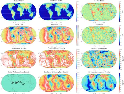
(a) Initial model used in the inversion. (b) Retrieved model parameters. (c) differences between the initial and final models. All fields have been interpolated to a 1° × 1° for illustration purposes.

Open in new tab Download slide

In Fig. 9 we compare the predictions of Moho depth from LithoRef18, LITHO1.0, CRUST1.0 and a recent gravity-derived global model (GEMMA; Reguzzoni & Sampietro 2015) against results from higher-resolution models informed by various seismic and/or potential field data in Australia (AusMoho; Kennett et al.2011), South America (GMSA12; van der Meijde et al.2013), Europe (EPcrust; Molinari & Morelli 2011), US (US-CrustVs-2015; Schmandt et al.2015), the North Atlantic (NAGTEC; Funck et al.2017) and continental China (China2014; He et al.2014). This comparison, although illustrative and informative, needs to be taken with caution, as (i) some of these regional models are actually either informed or constrained by CRUST1.0 (e.g. NAGTEC, EPcrust) and (ii) the latest updates of CRUST1.0 may include data either similar or identical to what was used in these studies (the full data set used in the latest versions of CRUST1.0 is not publicly available). It is not surprising then that CRUST1.0 shows the best agreement with the regional models, except in the case of GMSA12 (mostly constrained by gravity data), where our predictions agree slightly better than those of CRUST1.0. In all cases, however, the absolute mean discrepancy and the associated spread of LithoRef18 are comparable to those in CRUST1.0 and significantly smaller than those in the global GEMMA and LITHO1.0 models. In Africa, where seismic constraints are scarce, most recent models predict smaller crustal thickness values than those in CRUST1.0 (cf. van der Meijde et al.2015), and so does our model. In particular, our results are more similar to the models of Tugume et al. (2013) and Reguzzoni et al. (2013), which also used gravity data as constraints.

Figure 9.

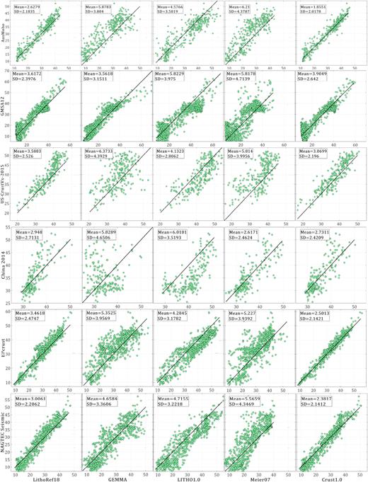
Comparison of predictions for crustal thickness (in km) from LithoRef18, GEMMA, Litho1.0 and CRUST1.0 against values given by regional, high-resolution models in Australia (AusMoho; Kennett et al.2011), South America (GMSA12; van der Meijde et al.2013), US (US-CrustVs-2015; Schmandt et al.2015), continental China (China2014; He et al.2014), Europe (EPcrust; Molinari & Morelli 2011) and the North Atlantic region (NAGTEC; Funck et al.2017). Each panel includes the mean of the point-wise discrepancies between the global and regional models as well as associated standard deviations (SD, a measure of dispersion). Smaller values of these two statistics indicate a closer agreement with the regional models.

Open in new tab Download slide

The results for the LAB depth show a modest variation within some continents, as per the original (seismic-based) restrictions in the inversion. Most of the change in LAB depths recorded in the oceans is concentrated at and around mid-ocean ridges (MORs). This is to be expected as the initial LAB in the oceans was based on a plate cooling model Grose & Afonso (2013) with the LAB beneath MORs set at 25 km depth everywhere (Section 2. We note that our final LAB depths resemble very closely those obtained from the multi-mode surface wave tomography model CAM2016Vsv (Ho et al.2016), as shown in http://ds.iris.edu/ds/products/emc-cam2016/.

The rest of the short wavelength variability related to sea mounts, oceanic plateaus and large fracture zones likely represents an upper bound in terms of lithospheric thickness. This is due to the combination of two factors. First, the oceanic Moho is in general poorly constrained by CRUST1.0. Second, we let the inversion to change the initial oceanic Moho only slightly, thus exaggerating changes in lithospheric thickness to fit the data. The use of more accurate estimates of Moho depths (Hoggard et al.2017) in the oceans could help in obtaining a more reliable LAB model; this is work in progress.

8.2.2 Crustal and mantle densities

The pattern and magnitude of crustal density in continents remained relatively similar to that in the starting model (Fig. 8C), with most of the differences being within ±50 kg m⁻³. However, these differences can be important in some cases (e.g. in gravity modelling), as they represent considerable changes in the average bulk density of a thick crust (i.e. their effect is integrated over the thickness of the entire continental crust). Most of the high amplitude differences are found in the oceans. Our model generally predicts lower densities along MORs and slightly higher densities in mature oceanic crust. Interestingly, LithoRef18’s density structure highlights features that were absent in the initial model. For instance, while the Walvis, Ninetyeast, Broken and Nazca ridges are indistinguishable in the initial density model, they are clearly visible in ours (Fig. 8B; see also Section 8.2.1). This is also the case in the other related parameters (i.e. LAB, Moho depth; see also Fig. 10). In continental interiors, LithoRef18 predicts somewhat higher average crustal densities than the input model. A comparison with higher-resolution density models in different parts of the world (e.g. Kozlovskaya et al.2004; Yegorova et al.2013; Hasterok & Gard 2016; Gradmann et al.2017; Sippel et al.2017; Alghamdi et al.2018; Wang et al.2018) shows a close agreement with our crustal density values.

Figure 10.

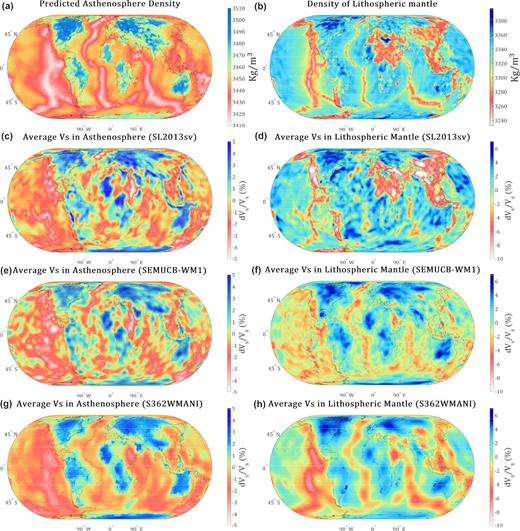
Comparison between the density structure of the lithosphere and sublithospheric upper mantle as predicted by LithoRef18 and seismic anomalies from three global tomography models: SL2013sv (Schaeffer & Lebedev 2013), SEMUCB-WM1 (French & Romanowicz 2014) and S362WMANI (Kustowsky et al. 2008). See text for details. All fields have been interpolated to a 1° × 1° for illustration purposes.

Open in new tab Download slide

The results for sublithospheric mantle density are shown in Fig. 8(B). The resulting density structure follows a pattern similar to that of lithospheric thickness. In this context, it is important to recall that the sublithospheric density values in Fig. 8(B) are the depth-averaged densities of the mantle between the LAB and the bottom of the model (410 km depth) and therefore there is an intrinsic ‘depth effect’ included in them (i.e. the average of an adiabatic density profile increases with average depth). The MORs are clearly distinguishable as relative low density zones, whereas stable continental areas with thick lithospheres are generally underlaid by higher density mantle. Although this is to be expected given the depth effect mentioned above, these observations raise the question of whether our results for the sublithospheric mantle are the product of real sensitivity to data or an artifact of the inversion/parametrization controlled somehow by the initial LAB depth. We discuss this further in the next section, where we show that our results are indeed supported by recent global seismic tomography models as well as by independent resolution analyses of gravity gradients and results from mineral physics.

The mean density of the lithosphere is not shown in Fig. 8 because it is not strictly part of the vector of model parameters m. However, it is an output of the model and therefore it is shown in Fig. 10 and discussed in the next section.

9 DISCUSSION

9.1 Lithospheric and sublithospheric densities: a comparison with seismic tomography models

If the density structure of LithoRef18 in the mantle is a reliable data-driven result and the density of the sublithospheric mantle is primarily controlled by temperature anomalies (a good first-order assumption), we should expect to see a correlation with seismic tomography models (i.e. high densities should correlate with regions of high seismic velocity and vice versa). Fig. 10 shows a comparison of our lithospheric and sublithospheric density models with three well-known global Vs tomography models (Kustowski et al.2008; Schaeffer & Lebedev 2013; French & Romanowicz 2014). Other models (e.g. SAVANI, GYPSUM, S40RTS, SEMUM2) show comparable features to those in Fig. 10 and therefore they are not shown here. In order to make a fair and valid comparison, the wavespeeds from all three tomography models were averaged over the same depth range as in our density models (i.e. the wavespeeds depicted in Fig. 10 do not represent wavespeeds at specific depths, but average values for the depth range LAB < d < 410 km depth).

All three tomographic models are shear wave velocity models, but differ in the data and methods used. SL2013sv (Schaeffer & Lebedev 2013) is an isotropic global upper mantle and transition zone Sv velocity model constrained by 521 705 vertical-component broad-band seismograms (selected from a data set of ∼3/4 million). It is based on a linearized (perturbation) inversion scheme (Schaeffer & Lebedev 2013), using a new 1-D reference model derived by these authors, and covers a period range from 11 to 450 sec with maximum estimated resolutions of ∼6°. SEMUCB-WM1 (French & Romanowicz 2014) is a global whole-mantle shear wave velocity model based on a ‘hybrid’ full-waveform approach that combines spectral finite element simulations of the wavefield (for the forward problem) with an iterative, nonlinear least-squares formalism. It is constrained by 447 800 waveforms from surface a body wave phases with an estimated maximum lateral resolution of ∼1200 km. S362WMANI (Kustowski et al.2008) is a whole-mantle anisotropic shear wave velocity model based on a waveform iterative linearized least-squares inversion of both surface and body wave data in which the 1-D reference model is updated at each iteration (similar to what is done here). Although no formal resolution analyses were provided, a nominal lateral resolution of ∼1000 km is claimed for the uppermost mantle.

Fig. 10 shows that all three tomography models agree well on the long-wavelength patterns of averaged velocity anomalies at both lithospheric and sublithospheric depths. The two most recent models, SL2013sv and SEMUCB-WM1, show the most agreement and a greater high-frequency content than S362WMANI. Although all three seismic models show a consistent structure to that in our density model of the lithosphere, the correlation between LithoRef18 with velocity anomalies in SL2013sv is the clearest (Table 7). This is somewhat expected given the role that this tomography model had in the initial LAB model (Section 2). We also note that except for SL2013sv (Schaeffer & Lebedev 2013), the other two models do not contain reliable/complete data at depths <50 km depth and therefore they do not show as detailed information as SL2013sv at shallow lithospheric depths (Figs 10D, F and H).

Table 7.

Open in new tab

Cross-correlation coefficients between lithospheric and sublithospheric densities and seismic velocity fields as shown in Fig. 10.

Tomography models	Lithospheric mantle density	Asthenosphere density
SL2013sv	0.7437	0.7860
SEMUCB-WM1	0.4092	0.7879
S362WMANI	0.5572	0.8067

Table 7.

Open in new tab

Cross-correlation coefficients between lithospheric and sublithospheric densities and seismic velocity fields as shown in Fig. 10.

Tomography models	Lithospheric mantle density	Asthenosphere density
SL2013sv	0.7437	0.7860
SEMUCB-WM1	0.4092	0.7879
S362WMANI	0.5572	0.8067

In the sublithospheric mantle, our density structure model correlates well with the pattern of seismic anomalies in the tomographic models, especially those in SL2013sv and SEMUCB-WM1. We recall here that the average density of the sublithospheric mantle (Figs 8B and 10A) was a free parameter in our inversion, not informed by seismic data. The fact that the retrieved density structure exhibits an excellent correlation with shear wave anomalies is a strong indication that the general pattern in our model is robust. Another piece of evidence that supports our suggestion that the retrieved sublithospheric density anomalies are the result of true sensitivity of the data is offered by (1) the fact that geoid anomalies are sensitive to deep density anomalies (Hager & Richards 1989; Bowin 1983, 2000; Featherstone 1997; Chase et al.2002; Afonso et al.2013b) and (2) the recent studies of Panet et al. (2014), Martinec (2014) and Greff-Lefftz et al. (2016b). These authors showed that satellite-derived gravity gradients have sensitivity to mantle mass anomalies down to mid-mantle depths. A last point worth mentioning is the fact that the absolute density values in the sublithospheric mantle retrieved by our inversion are in excellent agreement with estimates from seismic constraints (e.g. Kennett 1998) and from thermodynamic modelling of mantle rocks (e.g. Ganguly et al.2009; Chust et al.2017).

9.2 Using LithoRef18 to suppress far-field effects in regional studies

A common difficulty in any study that uses gravity information is the need to minimize the so-called edge or far-field effect, arising from the fact that the structure outside the model is not explicitly included in the modelling/inversion of the data. A common strategy to minimize this effect is to increase the size of the model (Aitken et al.2014; Szwillus et al.2016). This approach is valid when working with gravity anomalies, as the effect of unmodelled density anomalies tend to decay rapidly with distance (depending on the size of the density anomaly). However, despite unnecessarily increasing the computational cost, it is generally not a practical option when working with geoid height, gravity potential and/or long-wavelength gravity gradients as they are sensitive to density anomalies located relatively far from the modelled region (Szwillus et al.2016). Other options are possible. For instance, it is sometimes feasible to ‘copy’ or extend the density structure along the boundaries of the modelled region into a larger surrounding area (Zeyen & Fernàndez 1994; Fullea et al.2009; Afonso et al.2016b). This is more computationally efficient, but problematic when the outside region is highly heterogeneous. It thus becomes unclear how much the modelled structure is affected by the unmodelled ones or by the assumptions made about them (see Szwillus et al.2016,for a recent discussion).

The ideal situation is to have a way to account for the unmodelled structure at any distance from the region of interest as accurately as possible contingent on the goals of the study. We argue here that LithoRef18 is well suited to this end. We have prepared an easy-to-use, wrap-around code (both serial and parallel versions) that computes the contribution to gravity, geoid, and gravity gradients of the global structure at any observation point of interest (i.e. at any resolution). In this way, any local or regional model can be effectively embedded into the global LithoRef18 model and locally refined as desired while still accounting for the first-order density structure outside the modelled region. The user only needs to run the code once, indicating the boundaries of the domain of interest and the number and location of the observations points at which gravity, geoid or and/gravity gradients are required. These values can then be added to the contribution from the local structure as the latter is being refined by forward modelling or via an inversion algorithm; thus eliminating unnecessary domain extensions and/or assumptions about the density structure of the surrounding areas. The code can be downloaded at https://www.juanafonso.com/software or obtained from the first two authors upon request.

9.3 Future refinements

In this work, we restricted our attention to obtaining an internally consistent, first-order global model of the structure and density of the whole of the lithosphere and sublithospheric upper mantle on the basis of observable data (i.e. gravity anomalies, geoid heigh, absolute elevation and gravity gradients) and tenable prior information (e.g. seismic models, mantle composition). In doing so, the intended use of the model, available prior knowledge, parsimony of parameters, an computational complexity were the main guiding principles. Although the model so obtained is based on well-known geophysical principles and satisfies a large number of data, it is necessarily an approximation at best, and a physical abstraction at worst.

Specific areas for improvement that we will consider in the near future are:

The use of the full Marussi tensor: In this work we inverted for the diagonal terms of the Marussi tensor only. Although they do provide individual sensitivities, the diagonal terms are not all independent, as the trace of the tensor is zero. Including the off-diagonal components would therefore provide additional sensitivity to the modelled structures.
The use of an internally consistent data set, such as XGM2016 (Pail et al.2017) or the planned EGM2020, for gravity anomalies, geoid height and gravity gradients would help iron out potential inconsistencies that may arise from combining different data sets for these observables.
Expand the model parameter vector to include crustal thermal parameters and use surface heat flow data as an additional observable. However, we foresee advantages and drawbacks with this approach, as the uncertainties associated with this observable are large in most of the globe.
Include a more efficient surface grid and a dynamic parametrization of the sublithospheric mantle that will allow to subdivide the sublithospheric mantle into more than one region, thus making more efficient use of the sensitivity of the data sets and improving the model’s resolution/applicability. This is particularly important in regions with thin lithosphere.
In this study, we relied on a global compilation of crustal structure (CRUST1.0) and did not take full advantage of the most recent high-resolution regional seismic models based on dense arrays (e.g. US Array, ChinaArray, IberArray, etc.). Such regional models will be included as additional constraints in future releases of LithoRef18.
Modify the inversion scheme to formally include surface wave dispersion and receiver functions data into the inversion. This is perhaps the single most important improvement necessary to obtain a truly consistent global model. This will likely require the implementation of more comprehensive petrological and thermodynamic constraints into the inversion and model, but all the necessary components are in place (e.g. Schaeffer & Lebedev 2013; Afonso et al.2016a,b).

Also, as with any model made available to the scientific community, we plan to perform regular refinements to the model as more and/or better information becomes available to us. Finally, this work represents the necessary starting point towards a more ambitious reference model of the thermochemical structure of the Earth’s lithosphere and upper mantle based on multi-observable probabilistic tomography at global scale (Afonso et al.2013a,b; 2016b). This presents a grand challenge in terms of computational cost and algorithm development, but guided by the recent developments in reduced order modelling and parallel probabilistic techniques, we are confident that it will be a practical task in the next few years.

10 CONCLUSIONS

The main objective of this work was to derive a global lithospheric and upper mantle model that can serve as a reference/initial model for (i) higher-resolution gravity, seismological, geodetic and/or integrated geophysical studies of the lithosphere and upper mantle, (ii) accounting for far-field effects in regional gravity/geoid studies, (iii) regional and global geodynamic simulations where the effects of lithospheric structure are not negligible, (iv) assessing isostatic compensation mechanisms and estimates of residual, isostatic and dynamic topography, (v) stripping off the lithospheric signal in global estimates of the deep structure of the Earth and (vi) estimating boundary conditions for thermal modelling of sedimentary basins, among others. For this, we have simultaneously inverted global data sets of gravity anomalies, geoid height, absolute elevation, and gravity gradients with constraints from seismic models of the crust and mantle to derive a 2° × 2° global model (LithoRef18) of crustal thickness, average crustal density, lithospheric thickness, depth-dependent density of the lithospheric mantle, lithospheric geotherms, and average density of the sublithospheric mantle down to 410 km. The general inversion methodology presented in this work can also be applied in other planets for which potential field data are commonly the only (or main) constraint to their internal structures (e.g. Moon, Venus, etc.).

A comparison of LithoRef18’s predictions for crustal structure with recent higher-resolution regional models indicate that our model represents an improvement over other popular global crustal models. The LAB structure predicted by LithoRef18 is compatible with recent, high-resolution tomography models (e.g. Schaeffer & Lebedev 2013; French & Romanowicz 2014; Pasyanos et al.2014; Ho et al.2016), which makes it possible to combine these tomography models with LithoRef18 into a single density-seismic model compatible with a large number of seismic and potential field observations. Although this is not a completely satisfactory strategy, the strong similarities between LithoRef18 and e.g. SL2013sv (Schaeffer & Lebedev 2013) warrant it as a pragmatic approach especially in the context of serving as a starting models for detailed regional studies. Further efforts to produce internally consistent global reference models that honour multiple data sets of different nature (e.g. geochemistry, seismic, potential field, etc.; Afonso et al.2016b) will likely play a key role in improving our understanding of the complex physiochemical interactions between the lithosphere and the deep mantle.

SUPPORTING INFORMATION

Figure S1. Power spectrum of the harmonic degrees associated with a causative mass located at different depths inside the Earth. There is a rapid decrease in power up to degrees 8–10 for masses located below ∼400 km depth.

Figure S2. Total misfit associated with the joint inversion of gravity anomalies, geoid height, absolute topography and gravity gradients as a function of the degree and order of the applied filter. See Section 7.2 in the main text for details.

Figure S3. Square root of the degree of variance (m) of the filtered geoid (tapered as discussed in the main text) as function of spherical degree from anomalies located at different depth slices.

Figure S4. Top panel = predicted surface heat flow from LithoRef18; middle panel = predicted surface heat flow using the ‘mean’ method of Goutorbe et al. (2011); bottom panel = predicted surface heat flow using the ‘similarity’ method of Goutorbe et al. (2011).

Figure S5. Predicted Moho temperature from LithoRef18. Lithospheric geotherms can be easily computed from these values, the associated Moho depth, the LAB temperature (1300 °C) and LAB depths. All this information is contained in the distributed version of LithoRef18.

Figure S6. Comparison of predicted geoid heights due to a thin rectangular prism/tesseroid at different depths using three different approximations: a Cartesian prism approximation, a numerical tesseroid approximation (method of Grombein et al.2013) and our prism approximation described in Section 3.1.1. It can be seen that the tesseroid and the prism approximations are identical when the causative body is at a significant depth inside the planet, but they differ substantially (i.e. the tesseroid numerical approximation fails) when the causative body is at or near the surface of the planet (to make the comparison fair, we do not allow for subdivision of the causative mass as it would be done when using the numerical tesseroid approximation). In this case, the prism and Cartesian approximations agree well (as expected).

Figure S7. Relative errors (in per cent) in geoid, gravity and diagonal components of the gravity gradient tensor associated with the prism approximation to a tesseroid (these values are quoted in the main text).

Table S1. Total misfit associated with tests in Fig. 2.

Please note: Oxford University Press is not responsible for the content or functionality of any supporting materials supplied by the authors. Any queries (other than missing material) should be directed to the corresponding author for the paper.

ACKNOWLEDGEMENTS

We are indebted to H. Zeyen for sharing his codes and for suggestions on the inversion approach, to B. Steinberger for sharing his LAB models, and to A. Forte and an anonymous reviewer for their insightful reviews. The work of JCA has been supported by an ARC DP project (DP160103502) and CEED. JCA and FS acknowledge support from the ARC Centre of Excellence Core to Crust Fluids Systems (CCFS). JCA, FS, WS and JE acknowledge support from the Australia-Germany Joint Research Cooperation Scheme. This study has been done in the framework of the project ‘3D Earth - A Dynamic Living Planet’ funded by ESA as a Support to Science Element (STSE) and is contribution 1234 from the ARC Centre of Excellence for Core to Crust Fluid Systems (http://www.ccfs.mq..du.au) and 1273 in the GEMOC Key Centre (http://www.gemoc.mq.edu.au).

REFERENCES

Afonso

J.

,

Fullea

J.

,

Yang

Y.

,

Connolly

J.

,

Jones

A.

,

2013a

.

3-D multi-observable probabilistic inversion for the compositional and thermal structure of the lithosphere and upper mantle. II: general methodology and resolution analysis

,

J. geophys. Res.: Solid Earth

,

118

(

4

),

1650

–

1676

..

Afonso

J.C.

,

Fernàndez

M.

,

Ranalli

G.

,

Griffin

W.L.

,

Connolly

J.A.D.

,

2008

.

Integrated geophysical-petrological modeling of the lithosphere and sublithospheric upper mantle: methodology and applications

,

Geochem., Geophys., Geosyst.

,

9

(

5)

,

doi:10.1029/2007GC001834

.

Google Scholar

OpenURL Placeholder Text

WorldCat

Afonso

J.C.

,

Fullea

J.

,

Griffin

W.L.

,

Yang

Y.

,

Jones

A.G.

,

Connolly

J.A.D.

,

O’Reilly

S.Y.

,

2013b

.

3-D multiobservable probabilistic inversion for the compositional and thermal structure of the lithosphere and upper mantle. I: a priori petrological information and geophysical observables

,

J. geophys. Res.: Solid Earth

,

118

(

5

),

2586

–

2617

..

Afonso

J.C.

,

Moorkamp

M.

,

Fullea

J.

,

2016a

.

Imaging the Lithosphere and Upper Mantle

, pp.

191

–

218

.,

John Wiley & Sons, Inc

Google Scholar

Google Preview

OpenURL Placeholder Text

WorldCat

Afonso

J.C.

,

Rawlinson

N.

,

Yang

Y.

,

Schutt

D.L.

,

Jones

A.G.

,

Fullea

J.

,

Griffin

W.L.

,

2016b

.

3-D multiobservable probabilistic inversion for the compositional and thermal structure of the lithosphere and upper mantle: III. Thermochemical tomography in the Western-Central U.S

.,

J. geophys. Res.: Solid Earth

,

121

(

10

),

7337

–

7370

..

Afonso

J.C.

,

Rawlinson

N.

,

Yang

Y.

,

Schutt

D.L.

,

Jones

A.G.

,

Fullea

J.

,

Griffin

W.L.

,

2016c

.

3-D multiobservable probabilistic inversion for the compositional and thermal structure of the lithosphere and upper mantle: III. Thermochemical tomography in the Western-Central U.S

.,

J. geophys. Res.: Solid Earth

,

121

(

10

),

7337

–

7370

..

Afonso

J.C.

,

Ranalli

G.

,

2004

.

Crustal and mantle strengths in continental lithosphere: is the jelly sandwich model obsolete?

.

Tectonophysics

,

394

(

3-4

),

221

–

232

..

10.1016/j.tecto.2004.08.006

Aitken

A.

,

Altinay

C.

,

Gross

L.

,

2015

.

Australia’s lithospheric density field, and its isostatic equilibration

,

Geophys. J. Int.

,

203

(

3

),

1961

–

1976

..

Aitken

A.R.A.

et al. .,

2014

.

The subglacial geology of Wilkes Land, East Antarctica

,

Geophys. Res. Lett.

,

41

(

7

),

2390

–

2400

..

Alghamdi

A.H.

,

Aitken

A.R.A.

,

Dentith

M.C.

,

2018

.

The composition and structure of the deep crust of the capricorn orogen

,

Aust. J. Earth Sci.

,

65

(

1

),

9

–

24

..

10.1080/08120099.2018.1389769

Amante

C.

,

Eakins

B.

,

2009

.

ETOPO1 1 Arc-Minute Global Relief Model

.

Google Scholar

Google Preview

OpenURL Placeholder Text

WorldCat

Anderson

E.G.

,

1976

.

The Effect of Topography on Solutions of Stokes’ Problem

,

University of New South Wales

.

Google Scholar

Google Preview

OpenURL Placeholder Text

WorldCat

Asgharzadeh

M.F.

,

von Frese

R.R.B.

,

Kim

H.R.

,

Leftwich

T.E.

,

Kim

J.W.

,

2007

.

Spherical prism gravity effects by Gauss-Legendre quadrature integration

,

Geophys. J. Int.

,

169

(

1

),

1

–

11

.

Auer

L.

,

Boschi

L.

,

Becker

T.W.

,

Nissen-Meyer

T.

,

Giardini

D.

,

2014

.

Savani: a variable resolution whole-mantle model of anisotropic shear velocity variations based on multiple data sets

,

J. geophys. Res.: Solid Earth

,

119

(

4

),

3006

–

3034

..

Ballmer

M.D.

,

Ito

G.

,

van Hunen

J.

,

Tackley

P.J.

,

2011

.

Spatial and temporal variability in Hawaiian hotspot volcanism induced by small-scale convection

,

Nat. Geosci.

,

4

,

457

–

460

.

Balmino

G.

,

Vales

N.

,

Bonvalot

S.

,

Briais

A.

,

2012

.

Spherical harmonic modelling to ultra-high degree of Bouguer and isostatic anomalies

,

J. Geod.

,

86

(

7

),

499

–

520

..

10.1007/s00190-011-0533-4

Becker

T.W.

,

Faccenna

C.

,

Humphreys

E.D.

,

Lowry

A.R.

,

Miller

M.S.

,

2014

.

Static and dynamic support of western United States topography

,

Earth planet. Sci. Lett.

,

402

,

234

–

246

..

10.1016/j.epsl.2013.10.012

Blackford

L.S.

et al. .,

1997

.

{ScaLAPACK} Users’ Guide

,

Society for Industrial and Applied Mathematics

.

Google Scholar

Google Preview

OpenURL Placeholder Text

WorldCat

Bowin

C.

,

1983

.

Depth of principal mass anomalies contributing to the earth’s geoidal undulations and gravity anomalies∗

,

Mar. Geod.

,

7

(

1-4

),

61

–

100

..

10.1080/15210608309379476

Bowin

C.

,

2000

.

Mass anomaly structure of the Earth

,

Rev. Geophys.

,

38

(

3

),

355

–

387

..

Burov

E.

,

2011

.

Rheology and strength of the lithosphere

,

Mar. Petrol. Geol.

,

28

.

Google Scholar

OpenURL Placeholder Text

WorldCat

Cammarano

F.

,

Tackley

P.

,

Boschi

L.

,

2011

.

Seismic, petrological and geodynamical constraints on thermal and compositional structure of the upper mantle: global thermochemical models

,

Geophys. J. Int.

,

187

(

3

),

1301

–

1318

..

10.1111/j.1365-246X.2011.05223.x

Carlson

R.W.

,

Pearson

D.G.

,

James

D.E.

,

2005

.

Physical, chemical, and chronological characteristics of continental mantle

,

Rev. Geophys.

,

43

(

1

),

RG1001

,

doi:10.1029/2004RG000156

.

Chang

S.

,

Ferreira

A.M.G.

,

2017

.

Improving global radial anisotropy tomography: the importance of simultaneously inverting for crustal and mantle structureimproving global radial anisotropy tomography

,

Bull. seism. Soc. Am.

,

107

(

2

),

624

.

Chapman

D.

,

1986

.

Thermal gradients in the continental crust

, in

The Nature of the Lower Continental Crust

, Vol.

24

, pp.

63

–

70

.. eds

Dawson

J.

,

Carswell

D.

,

Hall

J.

,

Wedepohl

K.

,

Geol. Soc. Spec. Pub

Google Scholar

Google Preview

OpenURL Placeholder Text

WorldCat

Chase

C.G.

,

1985

.

The geological significance of the geoid

,

Ann. Rev. Earth planet. Sci.

,

13

(

1

),

97

–

117

..

10.1146/annurev.ea.13.050185.000525

Chase

C.G.

,

Libarkin

J.A.

,

Sussman

A.J.

,

2002

.

Colorado plateau: geoid and means of isostatic support

,

Int. Geol. Rev.

,

44

(

7

),

575

–

587

..

10.2747/0020-6814.44.7.575

Chust

T.C.

,

Steinle-Neumann

G.

,

Dolejš

D.

,

Schuberth

B.S.A.

,

Bunge

H.-P.

,

2017

.

Mma-eos: a computational framework for mineralogical thermodynamics

,

J. geophys. Res.: Solid Earth

,

122

(

12

),

9881

–

9920

..

Coblentz

D.

,

Chase

C.G.

,

Karlstrom

K.E.

,

van Wijk

J.

,

2011

.

Topography, the geoid, and compensation mechanisms for the southern Rocky Mountains

,

Geochem., Geophys., Geosyst.

,

12

(

4

),

doi:10.1029/2010GC003459

.

Google Scholar

OpenURL Placeholder Text

WorldCat

Crough

S.T.

,

Jurdy

D.M.

,

1980

.

Subducted lithosphere, hotspots, and the geoid

,

Earth planet. Sci. Lett.

,

48

(

1

),

15

–

22

..

10.1016/0012-821X(80)90165-X

Davies

J.H.

,

Davies

D.R.

,

2010

.

Earth’s surface heat flux

,

Solid Earth

,

1

(

1

),

5

–

24

..

Doin

M.-P.

,

Fleitout

L.

,

McKenzie

D.

,

1996

.

Geoid anomalies and the structure of continental and oceanic lithospheres

,

J. geophys. Res.: Solid Earth

,

101

(

B7

),

16119

–

16135

..

Featherstone

W.E.

,

1997

.

On the use of the geoid in geophysics: a case study over the North West Shelf of Australia

,

Explor. Geophys.

,

28

(

2

),

52

.

Flament

N.

,

Gurnis

M.

,

Muller

R.D.

,

2013

.

A review of observations and models of dynamic topography

,

Lithosphere

,

5

(

2

),

189

–

210

..

Forte

A.M.

,

Mitrovica

J.X.

,

Moucha

R.

,

Simmons

N.A.

,

Grand

S.P.

,

2007

.

Descent of the ancient Farallon slab drives localized mantle flow below the New Madrid seismic zone

,

Geophys. Res. Lett.

,

34

(

4

),

L04308

.

Forte

A.M.

,

Moucha

R.

,

Rowley

D.B.

,

Quéré

S.

,

Mitrovica

J.X.

,

Simmons

N.A.

,

Grand

S.P.

,

2009

.

Recent tectonic plate decelerations driven by mantle convection

,

Geophys. Res. Lett.

,

36

(

23

),

L23301

,

doi:10.1029/2009GL040224

.

Forte

A.M.

,

Perry

C. H.K.

,

2000

.

Geodynamic evidence for a chemically depleted continental tectosphere

,

Science

,

290

(

5498

),

1940

–

1944

.

French

S.W.

,

Romanowicz

B.A.

,

2014

.

Whole-mantle radially anisotropic shear velocity structure from spectral-element waveform tomography

,

Geophys. J. Int.

,

199

(

3

),

1303

–

1327

..

Fromm

T.

,

Jokat

W.

,

Behrmann

J.H.

,

2017

.

Interaction between a hotspot and a fracture zone: the crustal structure of walvis ridge at 6°E

,

Tectonophysics

,

716

,

108

–

120

..

10.1016/j.tecto.2017.03.001

Fullea

J.

,

Afonso

J.C.

,

Connolly

J.A.D.

,

Fernàndez

M.

,

García-Castellanos

D.

,

Zeyen

H.

,

2009

.

LitMod3D: an interactive 3-D software to model the thermal, compositional, density, seismological, and rheological structure of the lithosphere and sublithospheric upper mantle

,

Geochem., Geophys., Geosyst.

,

10

(

8

),

doi:10.1029/2009GC002391

.

Google Scholar

OpenURL Placeholder Text

WorldCat

Fullea

J.

,

Rodríguez-González

J.

,

Charco

M.

,

Martinec

Z.

,

Negredo

A.

,

Villaseñor

A.

,

2015

.

Perturbing effects of sub-lithospheric mass anomalies in GOCE gravity gradient and other gravity data modelling: application to the Atlantic-Mediterranean transition zone

,

Int. J. Appl. Earth Observ. Geoinform.

,

35

,

54

–

69

..

10.1016/j.jag.2014.02.003

Funck

T.

,

Geissler

W.H.

,

Kimbell

G.S.

,

Gradmann

S.

,

Erlendsson

Ö.

,

McDermott

K.

,

Petersen

U.K.

,

2017

.

Moho and basement depth in the ne atlantic ocean based on seismic refraction data and receiver functions

,

Geol. Soc., Lond., Spec. Publ.

,

447

(

1

),

207

–

231

..

Gallardo-Delgado

L.A.

,

Pérez-Flores

M.A.

,

Gómez-Treviño

E.

,

2003

.

A versatile algorithm for joint 3D inversion of gravity and magnetic data

,

Geophysics

,

68

(

3

),

doi:10.1190/1.1581067

.

Google Scholar

OpenURL Placeholder Text

WorldCat

Ganguly

J.

,

Freed

A.M.

,

Saxena

S.K.

,

2009

.

Density profiles of oceanic slabs and surrounding mantle: Integrated thermodynamic and thermal modeling, and implications for the fate of slabs at the 660km discontinuity

,

Phys. Earth planet. Inter.

,

172

(

3

),

257

–

267

..

10.1016/j.pepi.2008.10.005

Golle

O.

,

Dumoulin

C.

,

Choblet

G.

,

Čadek

O.

,

2012

.

Topography and geoid induced by a convecting mantle beneath an elastic lithosphere

,

Geophys. J. Int.

,

189

(

1

),

55

–

72

..

10.1111/j.1365-246X.2012.05364.x

Goutorbe

B.

,

Poort

J.

,

Lucazeau

F.

,

Raillard

S.

,

2011

.

Global heat flow trends resolved from multiple geological and geophysical proxies

,

Geophys. J. Int.

,

187

(

3

),

1405

–

1419

..

10.1111/j.1365-246X.2011.05228.x

Gradmann

S.

,

Haase

C.

,

Ebbing

J.

,

2017

.

Isostasy as a tool to validate interpretations of regional geophysical datasets—application to the mid-norwegian continental margin

,

Geol. Soc., Lond., Spec. Publ.

,

447

(

1

),

279

–

297

..

Green

D.H.

,

Falloon

T.J.

,

2015

.

Mantle-derived magmas: intraplate, hot-spots and mid-ocean ridges

,

Science Bulletin

,

60

,

1873

–

1900

.,

doi:10.1007/s11434-015-0920-y

.

Greff-Lefftz

M.

,

Métivier

L.

,

Panet

I.

,

Caron

L.

,

Pajot-Métivier

G.

,

Bouman

J.

,

2016a

.

Joint analysis of GOCE gravity gradients data of gravitational potential and of gravity with seismological and geodynamic observations to infer mantle properties

,

Geophys. J. Int.

,

205

(

1

),

257

–

283

..

Greff-Lefftz

M.

,

Métivier

L.

,

Panet

I.

,

Caron

L.

,

Pajot-Métivier

G.

,

Bouman

J.

,

2016b

.

Joint analysis of GOCE gravity gradients data of gravitational potential and of gravity with seismological and geodynamic observations to infer mantle properties

,

Geophys. J. Int.

,

205

(

1

),

257

–

283

..

Griffin

W.

,

O’Reilly

S.

,

Abe

N.

,

Aulbach

S.

,

Davies

R.

,

Pearson

N.

,

Doyle

B.

,

Kivi

K.

,

2003

.

The origin and evolution of Archean lithospheric mantle

,

Precamb. Res.

,

127

(

1-3

),

19

–

41

..

10.1016/S0301-9268(03)00180-3

Griffin

W.L.

,

O’Reilly

S.Y.

,

Afonso

J.C.

,

Begg

G.C.

,

2009

.

The composition and evolution of lithospheric mantle: a re-evaluation and its tectonic implications

,

J. Petrol.

,

50

(

7

),

1185

–

1204

..

10.1093/petrology/egn033

Grombein

T.

,

Seitz

K.

,

Heck

B.

,

2013

.

Optimized formulas for the gravitational field of a tesseroid

,

J. Geod.

,

87

(

7

),

645

–

660

..

10.1007/s00190-013-0636-1

Grose

C.J.

,

Afonso

J.C.

,

2013

.

Comprehensive plate models for the thermal evolution of oceanic lithosphere

,

Geochem., Geophys., Geosyst.

,

14

(

9

),

3751

–

3778

..

Grüninger

,

1990

,

Zur topographisch-isostatischen Reduktion der Schwere

,

PhD thesis

,

Universität Karlsruhe

.

Google Scholar

Google Preview

OpenURL Placeholder Text

WorldCat

Hager

B.H.

,

1984

.

Subducted slabs and the geoid: constraints on mantle rheology and flow

,

J. geophys. Res.: Solid Earth

,

89

(

B7

),

6003

–

6015

..

10.1029/JB089iB07p06003

Hager

B.H.

,

Richards

M.A.

,

1989

.

Long-wavelength variations in earth’s geoid: physical models and dynamical implications

,

Phil. Trans. R. Soc. A: Math., Phys. Eng. Sci.

,

328

(

1599

),

309

–

327

..

10.1098/rsta.1989.0038

Hasterok

D.

,

Chapman

D.S.

,

2007

.

Continental thermal isostasy: 1. Methods and sensitivity

,

J. geophys. Res.: Solid Earth

,

112

(

B6

).

Google Scholar

OpenURL Placeholder Text

WorldCat

Hasterok

D.

,

Gard

M.

,

2016

.

Utilizing thermal isostasy to estimate sub-lithospheric heat flow and anomalous crustal radioactivity

,

Earth planet. Sci. Lett.

,

450

,

197

–

207

..

10.1016/j.epsl.2016.06.037

Hawkesworth

C.J.

,

Cawood

P.A.

,

Dhuime

B.

,

2016

.

Tectonics and crustal evolution

,

GSA Today

,

26

(

09

),

4

–

11

..

Heck

B.

,

Seitz

K.

,

2007

.

A comparison of the tesseroid, prism and point-mass approaches for mass reductions in gravity field modelling

,

J. Geod.

,

81

(

2

),

121

–

136

..

10.1007/s00190-006-0094-0

He

R.

,

Shang

X.

,

Yu

C.

,

Zhang

H.

,

Van der Hilst

R.D.

,

2014

.

A unified map of moho depth and vp/vs ratio of continental china by receiver function analysis

,

Geophys. J. Int.

,

199

(

3

),

1910

–

1918

..

Hirt

C.

,

Kuhn

M.

,

2014

.

Band-limited topographic mass distribution generates full-spectrum gravity field: gravity forward modeling in the spectral and spatial domains revisited

,

J. geophys. Res.: Solid Earth

,

119

(

4

),

3646

–

3661

..

Hoggard

M.J.

,

Winterbourne

J.

,

Czarnota

K.

,

White

N.

,

2017

.

Oceanic residual depth measurements, the plate cooling model, and global dynamic topography

,

J. geophys. Res.: Solid Earth

,

122

(

3

),

2328

–

2372

.

Google Scholar

OpenURL Placeholder Text

WorldCat

Ho

T.

,

Priestley

K.

,

Debayle

E.

,

2016

.

A global horizontal shear velocity model of the upper mantle from multimode love wave measurements

,

Geophys. J. Int.

,

207

(

1

),

542

–

561

..

Ishii

M.

,

Tromp

J.

,

1999

.

Normal-mode and free-air gravity constraints on lateral variations in velocity and density of Earth’s mantle

,

Science (New York, N.Y.)

,

285

(

5431

),

1231

–

1236

..

10.1126/science.285.5431.1231

Jordan

T.H.

,

1988

.

Structure and formation of the continental tectosphere

,

J. Petrol.

,

Special_Volume

(

1

),

11

–

37

..

10.1093/petrology/Special_Volume.1.11

Kaban

M.K.

,

Schwintzer

P.

,

Reigber

C.

,

2004

.

A new isostatic model of the lithosphere and gravity field

,

J. Geod.

,

78

(

6

),

368

–

385

..

10.1007/s00190-004-0401-6

Kennett

B.L.N.

,

1998

.

On the density distribution within the earth

,

Geophys. J. Int.

,

132

(

2

),

374

–

382

..

10.1046/j.1365-246x.1998.00451.x

Kennett

B.L.N.

,

Salmon

M.

,

Saygin

E.

,

Group

A.W.

,

2011

.

AusMoho: the variation of Moho depth in Australia

,

Geophys. J. Int.

,

187

(

2

),

946

–

958

..

10.1111/j.1365-246X.2011.05194.x

Khan

A.

,

Kuvshinov

A.

,

Semenov

A.

,

2011

.

On the heterogeneous electrical conductivity structure of the Earth’s mantle with implications for transition zone water content

,

J. geophys. Res.

,

116

(

B1

),

B01103

.

Google Scholar

OpenURL Placeholder Text

WorldCat

Kozlovskaya

E.

,

Elo

S.

,

Hjelt

S.-E.

,

Yliniemi

J.

,

Pirttijärvi

M.

,

2004

.

3-D density model of the crust of southern and central Finland obtained from joint interpretation of the SVEKALAPKO crustal P-wave velocity models and gravity data

,

Geophys. J. Int.

,

158

(

3

),

827

–

848

..

10.1111/j.1365-246X.2004.02363.x

Kuhn

M.

,

2000

.

Geoidbestimmung unter Verwendung verschiedener Dichtehypothesen

,

PhD thesis

,

Deutsche Geodätische Kommission

,

München

.

Google Scholar

Google Preview

OpenURL Placeholder Text

WorldCat

Kuhn

M.

,

Featherstone

W.E.

,

2005

.

Construction of a synthetic earth gravity model by forward gravity modelling

, in

A Window on the Future of Geodesy

, pp.

350

–

355

.,

Springer-Verlag

.

Google Scholar

Google Preview

OpenURL Placeholder Text

WorldCat

Kuhn

M.

,

Seitz

K.

,

2005

.

Comparison of Newton’s integral in the space and frequency domains

, in

A Window on the Future of Geodesy

, pp.

386

–

391

.,

Springer-Verlag

.

Google Scholar

Google Preview

OpenURL Placeholder Text

WorldCat

Kustowski

B.

,

Ekström

G.

,

Dziewoński

A.M.

,

2008

.

Anisotropic shear-wave velocity structure of the Earth’s mantle: a global model

,

J. geophys. Res.

,

113

(

B6

),

B06306

.

Lachenbruch

A.H.

,

Morgan

P.

,

1990

.

Continental extension, magmatism and elevation; formal relations and rules of thumb

,

Tectonophysics

,

174

(

1-2

),

39

–

62

..

10.1016/0040-1951(90)90383-J

Laske

G.

,

Masters

G.

,

Ma

Z.

,

Pasyanos

M.

,

2013

.

Update on CRUST1.0—A 1-degree Global Model of Earth’s Crust

,

EGU General Assembly 2013

,

Vienna, Austria, EGU2013-2658

.

Google Scholar

Google Preview

OpenURL Placeholder Text

WorldCat

Lee

C.-T.A.

,

2003

.

Compositional variation of density and seismic velocities in natural peridotites at STP conditions: implications for seismic imaging of compositional heterogeneities in the upper mantle

,

J. geophys. Res.: Solid Earth

,

108

(

B9

),

doi:10.1029/2003JB002413

.

Google Scholar

OpenURL Placeholder Text

WorldCat

Lee

C.-T.A.

,

Luffi

P.

,

Chin

E.J.

,

2011

.

Building and destroying continental mantle

,

Ann. Rev. Earth planet. Sci.

,

39

(

1

),

59

–

90

..

10.1146/annurev-earth-040610-133505

Levandowski

W.

,

Jones

C.H.

,

Shen

W.

,

Ritzwoller

M.H.

,

Schulte-Pelkum

V.

,

2014

.

Origins of topography in the western U.S.: mapping crustal and upper mantle density variations using a uniform seismic velocity model

,

J. geophys. Res.: Solid Earth

,

119

(

3

),

2375

–

2396

..

Maceira

M.

,

Ammon

C.J.

,

2009

.

Joint inversion of surface wave velocity and gravity observations and its application to central Asian basins shear velocity structure

,

J. geophys. Res.

,

114

(

B2

),

B02314

.

Mader

K.

,

1951

.

Das Newtonsche Raumpotential prismatischer Körper und seine Ableitungen bis zur dritten Ordnung

,

Österreichische Zeitschrift für Vermessungswesen, Sonderheft 11

.

Google Scholar

Google Preview

OpenURL Placeholder Text

WorldCat

Marks

K.

,

Sandwell

D.T.

,

Vogt

P.R.

,

Hall

S.A.

,

1991

.

Mantle downwelling beneath the Australian-Antartic discordance zone: evidence from geoid height versus topography

,

Earth planet. Sci. Lett.

,

103

(

1–4

),

325

–

338

.

Martinec

Z.

,

2014

.

Mass-density Green’s functions for the gravitational gradient tensor at different heights

,

Geophys. J. Int.

,

196

(

3

),

1455

–

1465

..

McKenzie

D.

,

Bickle

M.J.

,

1988

.

The volume and composition of melt generates by extension of the lithosphere

,

J. Petrol.

,

29

,

625

–

679

.

McKenzie

D.

,

Jackson

J.

,

Priestley

K.

,

2005

.

Thermal structure of oceanic and continental lithosphere

,

Earth Planet. Sci. Lett.

,

233

,

337

–

349

.

Mechie

J.

,

Ben-Avraham

Z.

,

Weber

M.

,

Götze

H.-J.

,

Koulakov

I.

,

Mohsen

A.

,

Stiller

M.

,

2013

.

The distribution of Moho depths beneath the Arabian plate and margins

,

Tectonophysics

,

609

,

234

–

249

..

10.1016/j.tecto.2012.11.015

Menke

W.

,

2012

.

Geophysical Data Analysis: Discrete Inverse Theory

,

Academic Press

.

Google Scholar

Google Preview

OpenURL Placeholder Text

WorldCat

Molinari

I.

,

Morelli

A.

,

2011

.

Epcrust: a reference crustal model for the european plate

,

Geophys. J. Int.

,

185

(

1

),

352

–

364

..

10.1111/j.1365-246X.2011.04940.x

Molnar

P.

,

England

P.C.

,

Jones

C.H.

,

2015

.

Mantle dynamics, isostasy, and the support of high terrain

,

J. geophys. Res.: Solid Earth

,

120

(

3

),

1932

–

1957

..

Moorkamp

M.

,

Heincke

B.

,

Jegen

M.

,

Roberts

A.W.

,

Hobbs

R.W.

,

2011

.

A framework for 3-D joint inversion of MT, gravity and seismic refraction data

,

Geophys. J. Int.

,

184

(

1

),

477

–

493

..

10.1111/j.1365-246X.2010.04856.x

Motavalli-Anbaran

S.-H.

,

Zeyen

H.

,

Ebrahimzadeh Ardestani

V.

,

2013

.

3D joint inversion modeling of the lithospheric density structure based on gravity, geoid and topography data—application to the Alborz Mountains (Iran) and South Caspian Basin region

,

Tectonophysics

,

586

,

192

–

205

..

10.1016/j.tecto.2012.11.017

Müller

R.D.

,

Sdrolias

M.

,

Gaina

C.

,

Roest

W.R.

,

2008

.

Age, spreading rates, and spreading asymmetry of the world’s ocean crust

,

Geochem., Geophys., Geosyst.

,

9

(

4

),

doi:10.1029/2007GC001743

.

Google Scholar

OpenURL Placeholder Text

WorldCat

Nagy

D.

,

Papp

G.

,

Benedek

J.

,

2000

.

The gravitational potential and its derivatives for the prism

,

J. Geod.

,

74

(

7-8

),

552

–

560

..

10.1007/s001900000116

Novak

P.

,

Grafarend

E.W.

,

2005

.

Ellipsoidal representation of the topographical potential and its vertical gradient

,

J. Geod.

,

78

(

11-12

),

691

–

706

..

10.1007/s00190-005-0435-4

O'Reilly

S.Y.

,

Griffin

W.L.

,

2010

.

The continental lithosphere-asthenosphere boundary: can we sample it?

,

Lithos

,

120

,

1

–

13

.

O’Donnell

J.P.

,

Daly

E.

,

Tiberi

C.

,

Bastow

I.D.

,

O’Reilly

B.M.

,

Readman

P.W.

,

Hauser

F.

,

2011

.

Lithosphere-asthenosphere interaction beneath Ireland from joint inversion of teleseismic P-wave delay times and GRACE gravity

,

Geophys. J. Int.

,

184

(

3

),

1379

–

1396

..

10.1111/j.1365-246X.2011.04921.x

Pail

R.

,

Fecher

T.

,

Barnes

D.

,

Factor

J.F.

,

Holmes

S.A.

,

Gruber

T.

,

Zingerle

P.

,

2017

.

Short note: the experimental geopotential model XGM2016

,

J. Geod.

, pp.

1

–

9

.

Google Scholar

OpenURL Placeholder Text

WorldCat

Panet

I.

,

Pajot-Métivier

G.

,

Greff-Lefftz

M.

,

Métivier

L.

,

Diament

M.

,

Mandea

M.

,

2014

.

Mapping the mass distribution of Earth’s mantle using satellite-derived gravity gradients

,

Nat. Geosci.

,

7

(

2

),

131

–

135

..

Panning

M.

,

Romanowicz

B.

,

2006

.

A three-dimensional radially anisotropic model of shear velocity in the whole mantle

,

Geophys. J. Int.

,

167

(

1

),

361

–

379

.

Pasyanos

M.E.

,

Masters

T.G.

,

Laske

G.

,

Ma

Z.

,

2014

.

LITHO1.0: an updated crust and lithospheric model of the Earth

,

J. geophys. Res.: Solid Earth

,

119

(

3

),

2153

–

2173

..

Pavlis

N.K.

,

Holmes

S.A.

,

Kenyon

S.C.

,

Factor

J.K.

,

2012

.

The development and evaluation of the Earth Gravitational Model 2008 (EGM2008)

,

J. geophys. Res.: Solid Earth

,

117

(

B4

),

doi:10.1029/2011JB008916

.

Google Scholar

OpenURL Placeholder Text

WorldCat

Rawlinson

N.

,

Fichtner

A.

,

Sambridge

M.

,

Young

M.K.

,

2014

,

Seismic tomography and the assessment of uncertainty

, Vol.

55

, pp.

1

–

76

., ed.

Dmowska

R.

,

Advances in Geophysics

,

Elsevier

.

Google Scholar

Google Preview

OpenURL Placeholder Text

WorldCat

Reguzzoni

M.

,

Sampietro

D.

,

Sansò

F.

,

2013

.

Global Moho from the combination of the CRUST2.0 model and GOCE data

,

Geophys. J. Int.

,

195

(

1

),

222

–

237

..

Reguzzoni

M.

,

Sampietro

D.

,

2015

.

GEMMA: an Earth crustal model based on GOCE satellite data

,

Int. J. appl. Earth Observ. Geoinform.

,

35

,

31

–

43

..

10.1016/j.jag.2014.04.002

Ricard

Y.

,

Fleitout

L.

,

Froidevaux

C.

,

1984

.

Geoid heights and lithospheric stresses for a dynamic earth

,

Ann. Geophys.

,

2

,

267

–

286

.

Google Scholar

OpenURL Placeholder Text

WorldCat

Ritsema

J.

,

Deuss

A.

,

van Heijst

H.J.

,

Woodhouse

J.H.

,

2011

.

S40RTS: a degree-40 shear-velocity model for the mantle from new Rayleigh wave dispersion, teleseismic traveltime and normal-mode splitting function measurements

,

Geophys. J. Int.

,

184

(

3

),

1223

–

1236

..

10.1111/j.1365-246X.2010.04884.x

Rudnick

R.

,

Gao

S.

,

2003

.

Composition of the continental crust

, in

Treatise on Geochemistry

, pp.

1

–

64

.,

Elsevier

.

Google Scholar

Google Preview

OpenURL Placeholder Text

WorldCat

Sampietro

D.

,

2016

.

Crustal Modelling and Moho Estimation with GOCE Gravity Data

, pp.

127

–

144

.,

Springer

.

Google Scholar

Google Preview

OpenURL Placeholder Text

WorldCat

Schaeffer

A.J.

,

Lebedev

S.

,

2013

.

Global shear speed structure of the upper mantle and transition zone

,

Geophys. J. Int.

,

194

(

1

),

417

–

449

..

Schmandt

B.

,

Lin

F.-C.

,

Karlstrom

K.E.

,

2015

.

Distinct crustal isostasy trends east and west of the Rocky Mountain Front

,

Geophys. Res. Lett.

,

42

(

23

),

10 290

–

10 298

..

Shan

B.

,

Afonso

J.C.

,

Yang

Y.

,

Grose

C.J.

,

Zheng

Y.

,

Xiong

X.

,

Zhou

L.

,

2014

.

The thermochemical structure of the lithosphere and upper mantle beneath South China: results from multiobservable probabilistic inversion

,

J. geophys. Res.: Solid Earth

,

119

(

11

),

8417

–

8441

..

Shapiro

N.

,

Ritzwoller

M.

,

2004

.

Inferring surface heat flux distributions guided by a global seismic model: particular application to Antarctica

,

Earth planet. Sci. Lett.

,

223

,

213

–

224

.

Simmons

N.A.

,

Forte

A.M.

,

Boschi

L.

,

Grand

S.P.

,

2010

.

GyPSuM: a joint tomographic model of mantle density and seismic wave speeds

,

J. geophys. Res.

,

115

(

B12

),

B12310

,

doi:10.1029/2010JB007631

.

Simmons

N.A.

,

Forte

A.M.

,

Grand

S.P.

,

2006

.

Constraining mantle flow with seismic and geodynamic data: a joint approach

,

Earth planet. Sci. Lett.

,

246

(

1-2

),

109

–

124

..

10.1016/j.epsl.2006.04.003

Sippel

J.

,

Meeßen

C.

,

Cacace

M.

,

Mechie

J.

,

Fishwick

S.

,

Heine

C.

,

Scheck-Wenderoth

M.

,

Strecker

M.R.

,

2017

.

The kenya rift revisited: insights into lithospheric strength through data-driven 3-D gravity and thermal modelling

,

Solid Earth

,

8

(

1

),

45

–

81

..

Sjöberg

L.

,

Bagherbandi

M.

,

2011

.

A method of estimating the Moho density contrast with a tentative application of EGM08 and CRUST2.0

,

Acta Geophys.

,

59

(

3

),

502

–

525

..

10.2478/s11600-011-0004-6

Steinberger

B.

,

2007

.

Effects of latent heat release at phase boundaries on flow in the Earth’s mantle, phase boundary topography and dynamic topography at the Earth’s surface

,

Phys. Earth planet. Inter.

,

164

(

1-2

),

2

–

20

..

10.1016/j.pepi.2007.04.021

Steinberger

B.

,

2016

.

Topography caused by mantle density variations: observation-based estimates and models derived from tomography and lithosphere thickness

,

Geophys. J. Int.

,

205

(

1

),

604

–

621

..

Steinberger

B.

,

Becker

T.W.

,

2016

.

A comparison of lithospheric thickness models

,

Tectonophysics

,

746

,

325

–

338

.

Syracuse

E.

,

Zhang

H.

,

Maceira

M.

,

2017

.

Joint inversion of seismic and gravity data for imaging seismic velocity structure of the crust and upper mantle beneath utah, united states

,

Tectonophysics

,

718

,

105

–

117

..

10.1016/j.tecto.2017.07.005

Szwillus

W.

,

Ebbing

J.

,

Holzrichter

N.

,

2016

.

Importance of far-field topographic and isostatic corrections for regional density modelling

,

Geophys. J. Int.

,

207

(

1

),

274

–

287

..

Tarantola

A.

,

2005

.

Inverse Problem Theory

,

SIAM

.

Google Scholar

Google Preview

OpenURL Placeholder Text

WorldCat

Tiberi

C.

et al. .,

2008

.

Asthenospheric imprints on the lithosphere in Central Mongolia and Southern Siberia from a joint inversion of gravity and seismology (MOBAL experiment)

,

Geophys. J. Int.

,

175

(

3

),

1283

–

1297

..

10.1111/j.1365-246X.2008.03947.x

Tondi

R.

,

Cavazzoni

C.

,

Danecek

P.

,

Morelli

A.

,

2012

.

Parallel, ‘large’, dense matrix problems: application to 3D sequential integrated inversion of seismological and gravity data

,

Comput. Geosci.

,

48

,

143

–

156

..

10.1016/j.cageo.2012.05.026

Tondi

R.

,

Gilardoni

M.

,

Reguzzoni

M.

,

2017

.

The combined inversion of seismological and GOCE gravity data: new insights into the current state of the Pacific lithosphere and upper mantle

,

Tectonophysics

,

705

,

101

–

115

..

10.1016/j.tecto.2017.03.013

Torge

W.

,

2001

.

Geodesy

, 3rd Ed.,

deGruyter

,

Berlin

, pp.

431

.

Google Scholar

Google Preview

OpenURL Placeholder Text

WorldCat

Tork Qashqai

M.

,

Carlos Afonso

J.

,

Yang

Y.

,

2016

.

The crustal structure of the Arizona Transition Zone and southern Colorado Plateau from multiobservable probabilistic inversion

,

Geochem., Geophys., Geosyst.

,

17

:

(11)

,

4308

–

4332

.

Tugume

F.

,

Nyblade

A.

,

Julià

J.

,

van der Meijde

M.

,

2013

.

Precambrian crustal structure in africa and arabia: evidence lacking for secular variation

,

Tectonophysics

,

609

,

250

–

266

..

10.1016/j.tecto.2013.04.027

van der Meijde

M.

,

Fadel

I.

,

Ditmar

P.

,

Hamayun

M.

,

2015

.

Uncertainties in crustal thickness models for data sparse environments: a review for south america and africa

,

J. Geodyn.

,

84

,

1

–

18

.

van der Meijde

M.

,

Julià

J.

,

Assumpção

M.

,

2013

.

Gravity derived Moho for South America

,

Tectonophysics

,

609

,

456

–

467

..

10.1016/j.tecto.2013.03.023

Waldhauser

F.

,

Lippitsch

R.

,

Kissling

E.

,

Ansorge

J.

,

2002

.

High-resolution teleseismic tomography of upper-mantle structure using an a priori three-dimensional crustal model

,

Geophys. J. Int.

,

150

(

2

),

403

–

414

..

10.1046/j.1365-246X.2002.01690.x

Wangen

M.

,

2010

.

Physical Principles Of Sedimentary Basin Analysis

,

Cambridge University Press

.

Google Scholar

Google Preview

OpenURL Placeholder Text

WorldCat

Wang

X.

,

Holt

W.E.

,

Ghosh

A.

,

2015

.

Joint modeling of lithosphere and mantle dynamics: evaluation of constraints from global tomography models

,

J. geophys. Res.: Solid Earth

,

120

(

12

),

8633

–

8655

..

Wang

Z.

,

Fu

G.

,

She

Y.

,

2018

.

Crustal density structure, lithosphere flexure mechanism, and isostatic state throughout the qinling orogen revealed by in situ dense gravity observations

,

J. geophys. Res.: Solid Earth

,

123

(

11

),

10 026

–

10 039

.

Wild-Pfeiffer

F.

,

2008

.

A comparison of different mass elements for use in gravity gradiometry

,

J. Geod.

,

82

(

10

),

637

–

653

..

10.1007/s00190-008-0219-8

Yang

T.

,

Gurnis

M.

,

2016

.

Dynamic topography, gravity and the role of lateral viscosity variations from inversion of global mantle flow

,

Geophys. J. Int.

,

207

(

2

),

1186

–

1202

..

Yegorova

T.

,

Gobarenko

V.

,

Yanovskaya

T.

,

2013

.

Lithosphere structure of the Black Sea from 3-D gravity analysis and seismic tomography

,

Geophys. J. Int.

,

193

(

1

),

287

–

303

..

Zeyen

H.

,

Volker

F.

,

Wehrle

V.

,

Fuchs

K.

,

Sobolev

S.V.

,

Altherr

R.

,

1997

.

Styles of continental rifting: crust-mantle detachment and mantle plumes

,

Tectonophysics

,

278

(

1-4

),

329

–

352

..

10.1016/S0040-1951(97)00111-X

Zeyen

H.

,

Fernàndez

M.

,

1994

.

Integrated lithospheric modeling combining thermal, gravity, and local isostasy analysis: application to the NE Spanish Geotransect

,

J. geophys. Res.: Solid Earth

,

99

(

B9

),

18089

–

18102

..

Zlotnik

S.

,

Afonso

J.C.

,

Diez

P.

,

Fernandez

M.

,

2008

.

Small-scale gravitational instabilities under the oceans: implications for the evolution of oceanic lithosphere and its expression in geophysical observables

,

Phil. Mag.

,

88

,

3197

–

3217

.

APPENDIX A: PARALLEL IMPLEMENTATION OF THE INVERSION ALGORITHM

We use ScaLAPACK (Blackford et al.1997), a library of high-performance linear algebra routines, to deal with the large number and size of the matrix–matrix and vector–matrix multiplications needed in the inversion. Based on a first assessment of which parts of the algorithm were the most time-consuming, we chose to subdivide the inversion algorithm into a serial and a parallel part (see Fig. 5). In the serial part, predicted observations (forward modelling) and their contributions to the Jacobian matrix are computed, from which the misfit vector Δd^k [d^obs − g(m_k)] is obtained. At this stage, we distribute the Jacobian matrix and Δd^k to n processors to effectively divide the computational load among a 2-D grid of processors. We use the MPI library and BLACS communication environment for this purpose. All computations were performed with 576 processors [formed in 24P_ROWS × 24P_COLUMNS; Tondi et al. (2012)] given the limitations of our MG3 cluster.

The parallel computation part begins once the submatrices and subvectors are sent to the 2-D processor grid (Fig. 5. Each submatrix is handled by PBLAS (Parallel Basic Linear Algebra Subprogram) to perform the distributed vector–vector (PDSYMV), matrix–vector (PDGEMV) and matrix–matrix (PDGEMM) operations. Next, routine PDGESV is used to compute the (parallel) solution to the system of equations. Finally, each portion of the solution is returned by each processor to the serial part of the program for assembling the complete solution. Total execution time of the serial part is 2.8 × 10⁴ s and a full iteration of the inversion algorithm takes 3.4 × 10⁴ s. A further improvement in efficiency would involve parallelizing the serial part; this is work in progress. Used subroutines are available upon request from the authors.

APPENDIX B: MODEL RESOLUTION

A first order estimate of the independent resolution of model parameters by the inversion can be obtained by means of the so-called model resolution matrix or resolution operatorR. For our problem (see eqs 32–35), the resolution matrix can be written as (Tarantola 2005; Rawlinson et al.2014).

\begin{eqnarray*} {\bf R} = \biggr ( {\bf G}^{T}_{k} {\bf C}^{-1}_{D}{\bf G}_{k}+ {\bf C}^{-1}_{M}\biggr )^{-1} \biggr ({\bf G}^{T} {\bf C}^{-1}_{D} {\bf G} \biggr ). \end{eqnarray*}

(B1)

Therefore, R is a function of the data and prior information (or constraints) only. When the matrix |${\bf G}^{T}_{k} {\bf C}^{-1}_{D}{\bf G}_{k}$| is a regular matrix and the diagonal elements of |${\bf C}_{M}^{-1}$| are small, then R approaches the identity matrix, meaning that the model parameters can be estimated independently from each other. The farther R is from I, the worse the resolving power for parameters is (parameters are a ‘blurred’ version or a weighted average of the true ones). The effect of |${\bf C}_{M}^{-1}$| is critical; if a set of model parameters is considered ‘well constrained’ (i.e. the diagonal of |${\bf C}_{M}^{-1}$| is large as its variance is small), its corresponding elements in R will have values significantly smaller than 1, as the constraints effectively reduce their independence (see also Motavalli-Anbaran et al.2013). Fig. B1 shows the unnormalized elements of the main diagonal of R for the four main model parameters. The low values in the oceans reflect the relatively stringent constraints imposed during the inversion. Not surprisingly, the largest values are associated with the sublithospheric mantle density, which was the least constrained parameter. Although these plots could be also taken as an estimate of parameters’ uncertainties, this interpretation is likely to be, at least partially, flawed (Tarantola 2005; Motavalli-Anbaran et al.2013; Rawlinson et al.2014). A more informative exercise would be to run many (1000s) inversions randomly varying the starting model and parametrization/regularization and quantify the resulting variability in model parameters. Unfortunately, the computational cost of the inversions currently precludes us to perform such rigorous tests.

Figure B1.

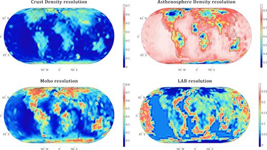
Representation of the resolution matrix R as plots of its (unnormalized) diagonal entries for the four main model parameters; higher values indicate better resolving power.

Open in new tab Download slide

This article is published and distributed under the terms of the Oxford University Press, Standard Journals Publication Model (https://dbpia.nl.go.kr/journals/pages/open_access/funder_policies/chorus/standard_publication_model)

Download all slides

Month:	Total Views:
March 2019	161
April 2019	192
May 2019	199
June 2019	87
July 2019	68
August 2019	48
September 2019	75
October 2019	58
November 2019	68
December 2019	31
January 2020	40
February 2020	53
March 2020	112
April 2020	76
May 2020	95
June 2020	96
July 2020	114
August 2020	106
September 2020	185
October 2020	128
November 2020	158
December 2020	91
January 2021	115
February 2021	89
March 2021	59
April 2021	46
May 2021	39
June 2021	32
July 2021	31
August 2021	40
September 2021	37
October 2021	41
November 2021	42
December 2021	37
January 2022	28
February 2022	27
March 2022	43
April 2022	49
May 2022	54
June 2022	82
July 2022	114
August 2022	108
September 2022	102
October 2022	122
November 2022	75
December 2022	108
January 2023	101
February 2023	113
March 2023	98
April 2023	120
May 2023	98
June 2023	83
July 2023	107
August 2023	61
September 2023	130
October 2023	143
November 2023	115
December 2023	79
January 2024	145
February 2024	97
March 2024	102
April 2024	122
May 2024	125
June 2024	177
July 2024	133
August 2024	105
September 2024	105
October 2024	115
November 2024	144
December 2024	113
January 2025	118
February 2025	127
March 2025	165
April 2025	151
May 2025	74

Article Contents

A global reference model of the lithosphere and upper mantle from joint inversion and analysis of multiple data sets

SUMMARY

1 INTRODUCTION

2 INPUT DATA SETS AND INITIAL MODEL

3 FORWARD PROBLEMS

3.1 Gravity, geoid and gravity gradients

3.1.1 The prism approximation

3.2 Isostatic elevation

4 TEMPERATURE, PRESSURE AND COMPOSITIONAL EFFECTS ON DENSITY

4.1 Geotherms and average lithospheric temperatures

4.2 Pressure

4.3 Compositional correction in cratonic regions

5 MODEL DISCRETIZATION AND MAIN FREE PARAMETERS

6 INVERSION STRATEGY

6.1 General problem formulation

6.2 Inversion algorithm

7 SYNTHETIC TESTS AND SENSITIVITY ANALYSIS

7.1 Global synthetic tests

7.2 Removing the effects of unmodelled density anomalies in the input data sets

8 RESULTS

8.1 Fits to data

8.2 Final model: LithoRef18

8.2.1 Crustal thickness and LAB structure

8.2.2 Crustal and mantle densities

9 DISCUSSION

9.1 Lithospheric and sublithospheric densities: a comparison with seismic tomography models

9.2 Using LithoRef18 to suppress far-field effects in regional studies

9.3 Future refinements

10 CONCLUSIONS

SUPPORTING INFORMATION

ACKNOWLEDGEMENTS

REFERENCES

APPENDIX A: PARALLEL IMPLEMENTATION OF THE INVERSION ALGORITHM

APPENDIX B: MODEL RESOLUTION

Supplementary data

Citations

Views

Altmetric

Email alerts

Astrophysics Data System

Citing articles via

Latest

Most Read

Most Cited

This Feature Is Available To Subscribers Only