Three-dimensional forward modelling of gravity data using mesh-free methods with radial basis functions and unstructured nodes

Long, Jianbo; Farquharson, Colin G

doi:10.1093/gji/ggz115

SUMMARY

A study is presented using a mesh-free approach and a radial basis function generated finite difference (RBF-FD) method for numerically modelling 3-D gravity data. The gravity responses, that is, vertical gravity and gravity gradients, are obtained by solving the partial differential equation (PDE), that is, the Poisson’s equation for gravitational potential. The mesh-free approach discretizes PDEs using exclusively a cloud of unconnected nodes, instead of traditional tessellated meshes as used by mesh-based numerical methods such as finite difference, finite element and finite volume. Thus, the potentially computationally expensive and unstable creation and manipulation of 3-D meshes can be entirely avoided. A new type of finite-smoothness radial basis functions (RBFs), namely, the quintic-order polyharmonic spline (PHS) RBF, is proposed here in the RBF-FD frame for solving the gravity problem. Previous geophysical data modelling studies using RBF-FD have employed the infinitely smooth RBFs, such as the popular Gaussian (GA) RBFs. Here, both GA and PHS RBFs were tested with different numbers of nodes per mesh-free subdomain and with various shape parameter values (only GA RBFs have a shape parameter). The test results show that the PHS RBF-FD method is more computationally efficient than the GA RBF-FD counterpart. To achieve more efficiency, unstructured node distributions are proposed in discretizing the density models. For both quasi-uniform and unstructured node distributions, numerical results from the proposed PHS RBF-FD demonstrate that the computed vertical gravity and gravitational potential values agree well with analytical solutions with a reasonable number of degrees of freedom. A comparison study of modelling a complex density model with the PHS RBF-FD scheme and nodal finite-element method shows that the RBF-FD scheme generates sparse, asymmetric, linear systems of equations, supports unstructured nodal discretization and local refinement, and can have nonlinear h-convergence under refinement. Finally, the proposed RBF-FD method was applied to obtain the vertical gravity and gravity gradients over a real-world density model, where the benefits of mesh-free discretization are clearly illustrated.

Gravity anomalies and Earth structure, Numerical modelling

1 INTRODUCTION

Gravity data interpretation by means of 3-D inversion in which 3-D subsurface density models are constructed using either a deterministic or a stochastic optimization method is a standard procedure (Moorkamp et al.2011). In the process of 3-D inversion, forward modelling of gravity data for a number of density models is necessary. There are basically two categories of methods for gravity forward modelling: summation-based techniques that evaluate volume integrals based on superposition principle and partial differential equation (PDE)-based techniques that solve a boundary value problem. In the former situation, the obtained solutions are often called closed-form, or analytical, solutions if the evaluation of integrals can be accurately carried out without using numerical quadrature. Early studies in terms of 3-D gravity data modelling mostly focused on the summation-based techniques, with a particular interest in using analytical formulae in conjunction with rectilinear meshes for discretizing the earth model (Nagy 1966; Banerjee & Das Gupta 1977; Last & Kubik 1983; Guillen & Menichetti 1984; Bear et al.1995; Li & Oldenburg 1998). To allow for more efficient forward modelling for complex density bodies, analytical formulae of gravity or gravitational potential for arbitrarily shaped, homogeneous polyhedral bodies, for example, tetrahedra, have also been developed (Paul 1974; Barnett 1976; Okabe 1979; Waldvogel 1979; Pohánka 1988; Petrović 1996; Holstein 2002; Tsoulis 2012; D'Urso 2014a). More recently, deriving analytical solutions assuming non-constant variation of density in polyhedral bodies has been attempted (Pohánka 1998; Hansen 1999; Holstein 2003; Zhou 2009; D'Urso 2014b; Ren et al.2017a). In the last situation, the inhomogeneous variation of density within polyhedral cells, which is typically described by polynomial functions, is considered to be more conformal to realistic density changes in some rock units such as sediments.

The most obvious advantage of the summation-based method is perhaps that numerical implementation is very straightforward. Also, accurate results can often be obtained for a given discretization of density model if analytical expressions are available. Another advantage is that for a minimum-structure style inversion, where only densities in each cell of the mesh are being varied while fixing the mesh itself, the resultant forward problem is linear (Li & Oldenburg 1998). However, one drawback of the summation-based approach is its relative inefficiency in the context of large-scale inversion. Particularly, the complexity of these algorithms grows as O(N × M), where N is the number of gravity data (measurements), and M is the number of cells of the mesh (degrees of freedom). Another disadvantage is that, when inverting large-scale gravity data using a standard gradient-based inversion algorithm, the sensitivity matrix is full and dense, and can require a large amount of memory to store. More details of this drawback are given by Farquharson & Mosher (2009) and May & Knepley (2011). To alleviate the computational complexity caused by a large and dense sensitivity matrix |$\mathbf {M}$|⁠, several mathematical tools have been developed. For example, wavelet transform methods have been used to compress the matrix |$\mathbf {M}$| (Li & Oldenburg 2003; Davis & Li 2011; Martin et al.2013); subspace techniques have been used to reduce the dimension of |$\mathbf {M}$| (Li & Oldenburg 1996; Barbosa et al.1997; Li & Oldenburg 1998); and fast multipole algorithms have been used to speed up the multiplication of |$\mathbf {M}$| with discretized density vector (May & Knepley 2011; Ren et al.2017b). Alternatively, data space approaches, which form a linear system of size N × N instead of M × M for the normal equations, with N ≪ M often in the 3-D case, can be used to reduce the memory storage during the inversion process (Chasseriau & Chouteau 2003; Pilkington 2009).

In contrast to the summation algorithms, the PDE-solving techniques synthesize all N gravity data at once, that is, their algorithm complexity is almost independent of the data amount. PDE-solving techniques have recently received increasing attention in gravity forward modelling and inversion (e.g. Zhang et al.2004; Cai & Wang 2005; Farquharson & Mosher 2009; May & Knepley 2011; Jahandari & Farquharson 2013; Gross et al.2015; Guzman 2015), although their implementations are not as straightforward as summation-based methods. In the PDE-based methods, gravity signals due to a density source are calculated by solving a differential equation for gravitational potential or gravity itself (Guzman 2015). Once a solution is obtained, one can calculate synthetic gravity signals everywhere in a trivial effort. The coefficient matrix of the linear system arising from solving the PDE is mostly very sparse, and when it is implicitly formed in a matrix-free way, the aforementioned sensitivity matrix |$\mathbf {M}$| even needs not to be explicitly stored. This enables very efficient computations involving the sensitivity matrix, for example, the product of |$\mathbf {M}$| with a vector |$\mathbf {b}$|⁠, in the case of gradient-based inversion (Farquharson & Mosher 2009), leaving the PDE-based methods an attractive option for large-scale gravity inversion problems.

Traditional PDE-based methods include finite-difference (FD) method, finite-volume (FV) method and finite-element (FE) method. FD approximates derivatives using difference equations and has the advantage of straightforward implementation. However, for irregular geometries, FD method requires non-trivial effort to accurately approximate curved boundaries in the mesh due to its reliance on tensor-product grids. In principle, FE and FV methods can be used for subsurface models with arbitrary geometries. Therefore, they offer the advantage of much greater flexibility in conforming to irregular geometries over the FD method. Examples of using FD techniques with rectilinear mesh in 3-D gravity data interpretation were given by Farquharson & Mosher (2009) for forward modelling and by Farquharson (2008) for inversion. Zhang et al. (2004) used an FE technique for gravity data modelling in their 3-D genetic inversion algorithm. They chose structured, rectilinear meshes in the FE discretization. Cai & Wang (2005) also studied FE methods with regular rectangular meshes in the 3-D gravity data modelling; there they conclude that the FE techniques can be significantly more efficient than summation-based techniques in modelling 3-D complex geological regions when the number of measurement stations is much greater than 100. Similar efficiency results between FE techniques and summation-based techniques were also reported by May & Knepley (2011). Their comparison study suggests that an approximated boundary condition of the far-field potential (Cai & Wang 2005) in conjunction with FE is more useful in practice than their summation-based methods and fast multipole method.

To fully take advantage of the flexibility in representing complicated geometries, Jahandari & Farquharson (2013) presented implementations of both FE and FV techniques with unstructured tetrahedral meshes in 3-D vertical gravity data modelling for a realistic geological model. They demonstrate the applicability of both techniques to complex structures. They also show the importance of local refinement around observation sites in the case of unstructured grids. In the context of inverting large-scale gravity gradient data, Haber et al. (2014) and Maag et al. (2017) used FV and FE techniques, respectively, to solve the 3-D forward modelling problem for efficiency. Both studies use rectilinear meshes in the model discretization. Gross et al. (2015) also presented an inversion technique for gravity and magnetic data, with their forward modelling parallelized and based on an FE implementation.

Integration of irregular geometries in the numerical modelling scheme is often desirable and important for accurately modelling real-world subsurface density models since these models are rarely made up of simple bricks or prisms. This is also true in the interpretation of many other geophysical data [e.g. direct current, electromagnetic (EM), seismic, etc.]. So far, it appears that FE and FV methods are the most intensively used PDE-solving methods when tackling complicated geometries of earth models. This is in a large part because of their efficiency and capability of conforming to geometry. First, both methods use local approximation to the PDEs, generating highly sparse linear systems that can be solved efficiently. Second, the construction of the local approximation by FE and FV, unlike that of FD method, is not restricted to the regular shape of elements or FV cells, although the approximation accuracy is affected by the regularity of the elements or cells. These two characteristics allow unstructured meshes to be easily used in discretization, and support local refinement that does not propagate to regions where refining is not needed. Thus, the degrees of freedom of the problem can be kept to a minimum. Applications of unstructured meshes using FE or FV methods have been reported in the forward modelling and inversion of, in addition to the gravity data, direct current resistivity data (Günther et al.2006; Rücker et al.2006), and EM data (Schwarzbach et al.2011; Ansari & Farquharson 2014; Usui 2015).

The above-mentioned traditional PDE-solving methods (FD, FE and FV) are essentially mesh-based methods as the unknown function of the problem is solved on a mesh topology. In this study, we propose to use a mesh-free, or meshless, method to forward model 3-D gravity data. Mesh-free methods are a branch of fundamentally different methods from mesh-based ones in that a PDE can be discretized into algebraic equations only by a number of scattered nodes without any tessellation (Nguyen et al.2008). As a result, the unknown quantity, for example, gravitational potential, is also solved on a set of scattered nodes. The discretization of an earth model can thus be greatly simplified, and does not need to be meshed in the way the mesh-based methods do. The removal of mesh is motivated by the following inherent mesh-associated difficulties in dealing with realistic earth models. The first difficulty is the non-trivial effort in adaptive remeshing or refining. Adaptive remeshing solves the problem of efficiently deploying sufficient but not redundant elements to regions where better numerical accuracy is needed. It is vital for computational efficiency as manual, pre-defined refinement is not practical for highly irregular earth models and can readily become untractable in an inversion problem in which candidate model geometry often varies progressively. However, adaptive remeshing schemes in the 3-D case face some drawbacks as explained next. A new mesh is obtained either by subdivision and/or merge of local elements (e.g. Key & Ovall 2011), or by remeshing the entire problem domain (e.g. Ren et al.2013). The former refining strategy is able to maintain the structure of the remaining part of the old mesh, but involves complicated mapping of elements between the two meshes. The latter strategy avoids the mapping process, but suffers from possible breakdown of mesh generator and can also be time-consuming as it requires a global meshing at each refinement. The second difficulty lies in the dilemma of ensuring sufficient quality of the mesh, or more precisely, quality of the elements. It is known that for FE and FV methods, solution accuracy and condition number of the linear system strongly depend on the quality of elements or cells (Du et al.2009; Jahandari & Farquharson 2013). However, generation of sufficient quality of the mesh often leads to overmeshed tiny cells around acute angles and joints of parametrized surfaces representing the geometry of different rock units (Nalepa et al.2016). This disadvantage will likely cause ill-conditioning of linear systems, and generate a large number of redundant cells.

All the above challenges in pursuing robust and quality model discretization can be greatly alleviated if only a cloud of unconnected nodes is required for a numerical solution. Since now, the removal or addition of some nodes is much easier. The representation of complex geometric features can be largely simplified since there can be much less quality requirements of node distribution in constructing function approximation, although the accuracy of the approximation is still affected by the quality of the node distribution. For example, in the 2-D case, three collinear points cannot be used to form an FE element and, therefore, FE approximation, and three non-collinear points cannot be used as a stencil in the classical grid-based FD method, but both nodal sets can be used to construct a mesh-free approximation if RBFs are used (the two mesh-free approximations may have different accuracies for a particular function). There are also less challenges in local refinement. For example, the local refinement does not affect the nodal distribution elsewhere, therefore, avoiding complicated mapping and possible geometric unconformity of the unknowns between the original discretization and the new one. Because of this, it is often unnecessary to regenerate the whole node discretization for a local refinement or coarsening. The generation of nodes in 3-D is typically faster than that of meshes and is less likely to suffer from breakdown. Node generation algorithms for mesh-free applications have received increasing attention recently (Du et al.2002; Fornberg & Flyer 2015b).

Mesh-free methods for solving PDEs have been developed with many variants since 1970s, however, their application in geophysical studies is still in its infancy. Jia & Hu (2006) applied an implementation of the element-free Galerkin technique, a weak form-based mesh-free method, to model and image 2-D seismic wave propagation. Wittke & Tezkan (2014) demonstrated an application of meshless local Petrov–Galerkin approach in 2-D magnetotelluric modelling. Martin et al. (2015) sucessfully used radial basis function generated finite differences (RBF-FDs) to obtain high-order convergence at material discontinuities in the numerical modelling of 2-D seismic wave field. Li et al. (2017) investigated the applicability of RBF-FDs in the time–space-domain elastic wave modelling, using the same radial function, that is, inverse multiquadric (MQ) RBF, as in Martin et al. (2015). Takekawa et al. (2015) and Takekawa & Mikada (2016) proposed a polynomial-based mesh-free FD method to simulate acoustic wave propagation in 2-D inhomogeneous media with curved interfaces, although the polynomial-based mesh-free FD approximation of derivatives is less robust than its RBF-based counterpart in terms of nodal distribution.

This study investigates the RBF-FD method in the 3-D gravity data modelling with a different type of RBFs from previous studies using RBF-FDs. Also, we demonstrate the applicability of our RBF-FD techniques with local refinements. As we will show later, RBF-FD method retains some advantages of the traditional mesh-based methods such as FE and FV. For example, it generates highly sparse linear systems, and allows easy representation of complicated geometries with unstructured nodes. Further, it has potential to overcome mesh-related difficulties in those methods: It has robust local approximation in terms of nodal distribution. It is our intention in this study to show that RBF-FD can be competitive with FE and FV techniques in forward modelling complex earth models, and hence be potentially advantageous over mesh-based methods for inversion problems.

2 THEORY

2.1 Poisson’s equation for gravitational potential

In the forward modelling of synthetic gravity signals due to a density distribution, the PDE-based methods solve the following gravitational potential equation (Kellogg 1967; Blakely 1996):

\begin{eqnarray*} \nabla ^2 \phi (\mathbf {r}) = -4 \pi \gamma \rho (\mathbf {r}); \quad \text{for} \quad \mathbf {r} \in \Omega \subset \mathbb {R}^3, \end{eqnarray*}

(1)

where ∇²ϕ is the Lapalcian of the potential ϕ expressed as a function of the position vector |$\mathbf {r}$|⁠, γ is the gravitational constant, and ρ denotes the density distribution function. This formula is valid both in and outside a source mass region, Ω_s⊂Ω, with Ω denoting an appropriate problem domain. The gravity field, or acceleration, |$\mathbf {g}$|⁠, is obtained by taking the gradient of ϕ:

\begin{eqnarray*} \mathbf {g} = - \nabla \phi . \end{eqnarray*}

(2)

In order to obtain a numerical solution to eq. (1), the problem domain is truncated to be a finite-length 3-D box in this study, denoted as Ω_p. Dirichlet boundary values

\begin{eqnarray*} \phi (\mathbf {r}) = 0, \quad \text{for} \quad \mathbf {r} \in \partial \Omega _{\mathrm{ p}}, \end{eqnarray*}

(3)

are used on all boundaries of Ω_p, assuming that the boundaries are set to be sufficiently far away from the source. One can try to use far-field approximated potential values as boundary values so that the computational domain is further reduced (Cai & Wang 2005). However, we found that the boundary condition in eq. (3) is simple to implement and more general for density sources with arbitrary shapes. Also, a local refinement with unstructured nodes allows for effective discretization without significant increase of degrees of freedom in our mesh-free implementation.

2.2 Mesh-free discretization

RBF-FD is one of the mesh-free techniques using the strong form of PDEs and solves differential equations in a classical FD way (Flyer et al.2014). It generalizes classical grid-based FD methods from lattice-based stencils to arbitrarily scattered nodal subdomains (Fig. 1). A key feature of mesh-free discretizations is that the mesh used for describing an earth model, which can be, for example, a mesh generated from geological modelling with the interfaces of rock units being triangulated but the interior of each rock unit not tessellated, and the mesh used for discretizing the PDEs are decoupled. These two meshes would be the same in the traditional mesh-based numerical modelling methods, in which all the interior regions of rock units also need to be meshed, and the physical property value in each cell of the mesh is typically assigned as a constant (but different cells can have different values). However, in the mesh-free case, the ‘mesh’ used for discretizing the mathematical equations is just only a cloud of nodes. Thus, each node is associated with a physical property value, which is required to obtain a numerical solution and can be sampled from the mesh of model discretization according to where the node is located in that model mesh. Consequently, curved boundaries and interfaces consistent with geological models no longer need to be approximated by a surface mesh such as triangulation.

Figure 1.

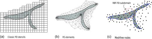
Schematic illustration of model discretization for 2-D irregular geometries using (a) grid-based (quad-tree) FD mesh, (b) unstructured FE elements and (c) mesh-free nodes. In the mesh-free RBF-FD case, nodes (the blue ones here) can be arranged arbitrarily to conform to the geometries of an object in the earth model, while in the classic FD case curves and segments not parallel to Cartesian grids have to be approximated in a staircase manner.

Open in new tab Download slide

For each node, a mesh-free subdomain is constructed as a local subdomain that contains a certain number of nodes in the vicinity of that node (called central, or support node). Unlike classical FD stencils and FE elements that have specific geometries (e.g. cubes and tetrahedra in the 3-D case), mesh-free subdomains typically have no fixed geometric structures; it is the amount of nodes in each subdomain that matters (Fig. 1c). In RBF-FD, radial basis functions (RBFs) are employed to construct local approximation in each local subdomain in which the number of nodes is far less than the total number of nodes of the model. This feature of RBF-FD methods ensures that a sparse linear system of equations is generated after approximating the PDEs. Theoretically, the number of nodes in each subdomain, n, is not necessarily the same. For the sake of easy implementation, we set the number of nodes in every RBF-FD subdomain as the same n, and the subdomains are formed by finding the n − 1 nearest nodes of each support node using a k-dimensional tree search algorithm (Kennel 2004). The closeness is measured by the standard Euclidean distance among nodes.

2.3 RBFs

Several popular methods used for carrying out function approximation in the mesh-free way include moving least squares (MLS; Belytschko et al.1994), reproducing kernel particle methods (Liu et al.1995), and RBFs (Powell 1990). A prominent feature of using RBFs is that the resultant approximant satisfies the Kronecker delta function properties, that is, the approximant |$\hat{\phi }$| of an unknown function ϕ passes through all data values ϕ_i (i = 1, 2, …, n): |$\hat{\phi }(\mathbf {r}_{i}) = \phi _{i} = \phi (\mathbf {r}_{i})$|⁠. The use of RBFs in mesh-free PDE-solving techniques thus enables a simple treatment of Dirichlet-type boundary conditions, for which special boundary treatments would otherwise be needed if using polynomial-based approximation (Atluri & Shen 2002). Another advantage of using RBFs is their natural independence on the spatial dimension as all RBFs are radially symmetric about a central spatial position (Powell 1990; Buhmann 2003). This is an important property to guarantee non-singularity of multidimensional mesh-free interpolation even for cases of extreme nodal arrangements (e.g. inline nodes in Fig. 2), which will cause singularity issue in polynomial-only methods such as MLS (Wang & Liu 2002a).

Figure 2.

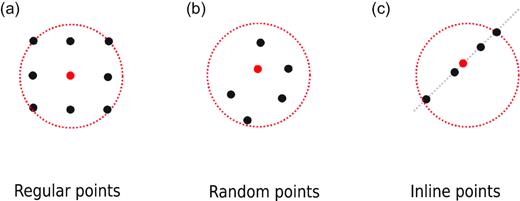
Some nodal arrangements in a 2-D mesh-free subdomain: (a) regular, equidistant nodes, (b) randomly distributed nodes and (c) collinear nodes.

Open in new tab Download slide

Many different types of RBFs have been proposed to solve PDEs in mesh-free applications over the past two decades (Fasshauer 2007; Nguyen et al.2008; Chen et al.2017). Some common RBFs are given in Table 1 and are grouped here as two categories in terms of smoothness: infinitely smooth and finite-smoothness RBFs (the finite-smoothness RBFs are sometimes called piecewise smooth RBFs, see Fornberg et al.2002). The former type of RBFs is widely used in many different mesh-free PDE-solving scenarios since the pioneering work by Kansa (1990a,b). The success of infinitely smooth RBFs is largely due to their superior convergence rate in interpolation with scattered data points (Hardy 1971; Fornberg & Flyer 2015a). However, infinitely smooth RBFs often contain a shape parameter (see Table 1) that controls the function’s flatness. It is well known that in the case of using infinitely smooth RBFs without any modification, flat RBFs will lead to better local interpolation accuracy in theory but also a very ill-conditioned linear system in the function approximation, a phenomenon recognized as ‘uncertainty principle’ in the literature (Schaback 1995; Fasshauer & Zhang 2007). If the ill-conditioned local system is solved directly using algorithms with finite precision arithmetics, one eventually obtains numerical results with very poor interpolation accuracy. Numerous efforts have been devoted to overcoming this difficulty, and they can be grouped as either via searching an ‘optimal’ or trade-off shape parameter before the solution from directly solving the linear system of equations deteriorates (hereafter called RBF-direct method, Rippa 1999; Wang & Liu 2002b; Fasshauer & Zhang 2007; Davydov & Oanh 2011; Uddin 2014), or via changing the original RBF bases spanning the solution space in order to form a set of more stable bases before solving the local linear system (Fornberg & Wright 2004; Fornberg & Piret 2007; Fornberg et al.2011; Fasshauer & McCourt 2012; Fornberg et al.2013). Despite these efforts, finding an efficient and general strategy to determine the shape parameter in the context of solving PDEs is still unresolved. This is because of drawbacks for both strategies in the above efforts: the ‘optimal shape parameter’ method often suffers from a lack of good error estimators before determining the unknown function in a boundary value problem. An optimal shape parameter is often affected by many factors including nodal arrangement, type of RBFs, subdomain size and the unknown function itself (Rippa 1999), making the search algorithms too problem-specific and impractical in the realistic modelling problems. The basis-changing method provides stable solutions for a very large range of shape parameter, however, it often involves complicated decomposition and orthogonalization of original interpolating matrix, and could cost 10–20 times more computational time than using RBF-direct methods (Larsson et al.2013).

Table 1.

Open in new tab

Common types of RBFs. The infinitely differentiable RBFs include a shape parameter c > 0. r is the Euclidean distance between two points |$\mathbf {r}_1$| and |$\mathbf {r}_2$|⁠: |$r = || \mathbf {r}_1 - \mathbf {r}_2 ||_{l_2}$|⁠.

Type of basis function	Radial function R(r)
Finite-smoothness RBFs
Generalized Duchon spline	r^2klogr, k ∈ N⁺
Polyharmonic spline (PHS)	r^k, 0 < k∉2N⁺
Infinitely smooth RBFs
Gaussian (GA)	\|$e^{-(c r)^2}$\|
Multiquadric (MQ)	\|$(c^2 + r^2)^{\frac{1}{2}}$\|
Inverse-multiquadric (IMQ)	\|$({c^2 + { r}^2})^{-\frac{1}{2}}$\|

Type of basis function	Radial function R(r)
Finite-smoothness RBFs
Generalized Duchon spline	r^2klogr, k ∈ N⁺
Polyharmonic spline (PHS)	r^k, 0 < k∉2N⁺
Infinitely smooth RBFs
Gaussian (GA)	\|$e^{-(c r)^2}$\|
Multiquadric (MQ)	\|$(c^2 + r^2)^{\frac{1}{2}}$\|
Inverse-multiquadric (IMQ)	\|$({c^2 + { r}^2})^{-\frac{1}{2}}$\|

Table 1.

Open in new tab

Common types of RBFs. The infinitely differentiable RBFs include a shape parameter c > 0. r is the Euclidean distance between two points |$\mathbf {r}_1$| and |$\mathbf {r}_2$|⁠: |$r = || \mathbf {r}_1 - \mathbf {r}_2 ||_{l_2}$|⁠.

Type of basis function	Radial function R(r)
Finite-smoothness RBFs
Generalized Duchon spline	r^2klogr, k ∈ N⁺
Polyharmonic spline (PHS)	r^k, 0 < k∉2N⁺
Infinitely smooth RBFs
Gaussian (GA)	\|$e^{-(c r)^2}$\|
Multiquadric (MQ)	\|$(c^2 + r^2)^{\frac{1}{2}}$\|
Inverse-multiquadric (IMQ)	\|$({c^2 + { r}^2})^{-\frac{1}{2}}$\|

Type of basis function	Radial function R(r)
Finite-smoothness RBFs
Generalized Duchon spline	r^2klogr, k ∈ N⁺
Polyharmonic spline (PHS)	r^k, 0 < k∉2N⁺
Infinitely smooth RBFs
Gaussian (GA)	\|$e^{-(c r)^2}$\|
Multiquadric (MQ)	\|$(c^2 + r^2)^{\frac{1}{2}}$\|
Inverse-multiquadric (IMQ)	\|$({c^2 + { r}^2})^{-\frac{1}{2}}$\|

Finite-smoothness RBFs (e.g. polyharmonic splines, PHSs), on the other hand, are free of such a shape parameter. This is a promising advantage compared with infinitely smooth RBFs in our application since the difficulty of selecting a good shape parameter is completely avoided. Historically, the finite-smoothness RBFs were not used as widely as the infinitely smooth ones in PDE-solving applications. This is because of two reasons (Iske 2003): First, finite-smoothness RBFs all have a finite order of smoothness, therefore, a finite order of convergence for smooth function approximation; second, not all of finite-smoothness RBFs are positive definite functions, meaning using some of the RBFs alone may result in singularity of the interpolation matrix even for a regular point set. Nevertheless, the non-singularity can be assured when the interpolation is enriched with polynomials, except for extreme nodal arrangements such as collinear nodes in 2-D and 3-D spaces or coplanar nodes in the 3-D case (see Fig. 2 and more rigorous definition in Buhmann 2003). However, these extreme scenarios are almost certainly avoided in our application because of the manner in which the neighbouring nodes are chosen to construct local subdomains in this study. Additionally, recent studies (Flyer et al.2016a,b; Bayona et al.2017) show that the interpolation using PHS RBFs, if augmented by appropriate polynomials, are not only able to avoid the singularity on practical node arrangements in any number of spatial dimension, but also can overcome saturation errors under local refinement of nodes in subdomains, a difficulty often encountered when using infinitely smooth RBFs alone such as Gaussian (GA) radial functions (Fornberg et al.2013). So far, the infinitely smooth RBFs have been dominantly used in RBF-FD methods. This motivates us to give examples in this study of using both types of RBFs (GA and PHS) in our RBF-FD implementation to illustrate (1) how the RBF-FD can work for both of them, (2) the difference between using the two different RBFs and (3) the advantages gained using PHS RBFs.

2.4 RBF-FD

In RBF-FD, differential equations are approximated by an RBF-based interpolant and are set to hold at the support node of each subdomain. RBF interpolation is formed as a linear combination of the translates of a single RBF, |$R(|| \mathbf {r} - \mathbf {r}_{k} ||)$|⁠, that collocates the sample data |${\lbrace f_{k}\rbrace }^{n}_{k=1}$| in a local subdomain at the included nodes |${\lbrace \mathbf {r}_{k}\rbrace }^{n}_{k=1}$|⁠, |$\mathbf {r}_{k} \in \ \mathbb {R}^3$|⁠. The interpolant |$s(\mathbf {r})$| is written as

\begin{eqnarray*} s(\mathbf {r}) = \sum ^{n}_{k=1} R(|| \mathbf {r} - \mathbf {r}_{k} ||) \cdot c_{k}, \end{eqnarray*}

(4)

where || · || is the l₂ norm. The interpolation coefficients, c_k, are sought by enforcing the standard Lagrange interpolation conditions:

\begin{eqnarray*} s(\boldsymbol {r}_{k}) = f_{k}, \quad \quad k = 1,2,\cdots , n, \end{eqnarray*}

(5)

which is equivalent to solving the following local linear system:

\begin{eqnarray*} { {\begin{pmatrix}R(||\mathbf {r}_1 - \mathbf {r}_1||) & \quad R(||\mathbf {r}_1 - \mathbf {r}_2||) & \quad \cdots & \quad R(||\mathbf {r}_1 - \mathbf {r}_n||) \\ R(||\mathbf {r}_2 - \mathbf {r}_1||) & \quad R(||\mathbf {r}_2 - \mathbf {r}_2||) & \quad \cdots & \quad R(||\mathbf {r}_2 - \mathbf {r}_n||) \\ \vdots & \quad \vdots & \quad \ddots & \quad \vdots \\ R(||\mathbf {r}_n - \mathbf {r}_1||) & \quad R(||\mathbf {r}_n - \mathbf {r}_2||) & \quad \cdots & \quad R(||\mathbf {r}_n - \mathbf {r}_n||) \end{pmatrix}} {\begin{pmatrix}c_1 \\ c_2 \\ \vdots \\ c_n \end{pmatrix}} = {\begin{pmatrix}f_1 \\ f_2 \\ \vdots \\ f_n \end{pmatrix}}}. \end{eqnarray*}

(6)

The compact matrix form of eq. (6) can be written as

\begin{eqnarray*} \mathbf {K} \mathbf {c} = \mathbf {F}, \end{eqnarray*}

(7)

where |$\mathbf {K}$| is the symmetric matrix of the left-hand side of eq. (6), |$\mathbf {c} = [c_1 \,\, c_2 \,\, \cdots \,\, c_n]^{T}$| is the vector of coefficients and |$\mathbf {F} = [f_1 \,\, f_2 \,\, \cdots \,\, f_n]^{T}$| is the data vector. Hereinafter, the superscript, T, denotes the transpose of a vector or matrix.

The interpolation in eq. (4) is often enriched with low-order polynomial functions, in conjunction with matching constraints on the expanded coefficients, though the purpose of enrichment is not always the same for GA and PHS RBFs (Flyer et al.2014). In general, the enrichment of low-order polynomials improves accuracy of approximating constant or nearly constant functions. In the 3-D case, a basis of linear polynomials is [1, x, y, z] and [1, x, y, z, xy, yz, xz, x², y², z²] for quadratic polynomials. Thus, including up to linear polynomials in eq. (4) leads to

\begin{eqnarray*} s(\mathbf {r}) = \sum ^{n}_{k=1} R(|| \mathbf {r} - \mathbf {r}_{k} ||) \cdot c_{k} + d_{0} + d_{1}x + d_{2}y + d_{3}z, \end{eqnarray*}

(8)

with d_i, i = 0, 1, 2, 3 as extra degrees of freedom. According to the unisolvency condition (Buhmann 2003), the constraints

\begin{eqnarray*} \sum ^{n}_{k=1}c_{k} = \sum ^{n}_{k=1}c_{k}x_{k} = \sum ^{n}_{k=1}c_{k}y_{k} = \sum ^{n}_{k=1}c_{k}z_{k} = 0 \end{eqnarray*}

(9)

satisfied at the n nodes are required to obtain a unique solution to the interpolant in eq. (8). Here, x_k, y_k and z_k are the Cartesian coordinates of the kth node. The enriched linear system then becomes

\begin{eqnarray*} {\begin{pmatrix}& & & | & 1 & x_{1} & y_{1} & z_{1} \\ & \mathbf {K} & & | & \vdots & \vdots & \vdots & \vdots \\ & & & | & 1 & x_{n} & y_{n} & z_{n} \\ - & - & - & + & - & - & - & - \\ 1 & \cdots & 1 & | & & & & \\ x_{1} & \cdots & x_{n} & | & & \mathbf {0} & & \\ y_{1} & \cdots & y_{n} & | & & & & \\ z_{1} & \cdots & z_{n} & | & & & & \end{pmatrix}} {\begin{pmatrix}c_1 \\ \vdots \\ c_n \\ - \\ d_{0} \\ d_{1} \\ d_{2} \\ d_{3} \end{pmatrix}} = {\begin{pmatrix}f_1 \\ \vdots \\ f_n \\ - \\ 0 \\ 0 \\ 0 \\ 0 \end{pmatrix}}, \end{eqnarray*}

(10)

and can be expressed in a more compact matrix form:

\begin{eqnarray*} {\begin{pmatrix}\mathbf {K} & \mathbf {P} \\ \mathbf {P}^{T} & \mathbf {0} \end{pmatrix}} {\begin{pmatrix}\mathbf {c} \\ \mathbf {d} \end{pmatrix}} = {\begin{pmatrix}\mathbf {F} \\ \mathbf {0} \end{pmatrix}}, \end{eqnarray*}

(11)

where |$\mathbf {P}$| denotes the upper right blocky matrix with polynomial entries in the coefficient matrix of eq. (10) and |$\mathbf {d}$| denotes the vector [d₀ d₁ d₂ d₃]^T.

In our implementation, within each RBF-FD subdomain, the Laplacian operator from the PDE for the potential, that is, eq. (1), is approximated at the support node by a linear combination of potential values, ϕ_k, at the n nodes, that is, the nodes in the subdomain compose the RBF-FD ‘stencil’:

\begin{eqnarray*} \nabla ^{2} \phi (\mathbf {r}_{i}) = \sum ^{n}_{k=1} w_{k} \phi _{k} = -4 \pi \gamma \rho (\mathbf {r}_{i}), \end{eqnarray*}

(12)

where |$\mathbf {r}_{i}$| is the position of the selected support node (Fig. 3) and w_k are the coefficients or RBF-FD weights. |$\rho (\mathbf {r}_{i})$| is the sampled density value at |$\mathbf {r}_{i}$|⁠. If the support node is located on the interface between two homogeneous regions, |$\rho (\mathbf {r}_{i})$| is taken as the averaged value of the two densities of the two regions: (ρ₁ + ρ₂)/2. It can be readily verified that w_k is obtained by solving a local linear system with the same left-hand-side matrix as in eq. (10), but with a different right-hand-side vector:

\begin{eqnarray*} {\begin{pmatrix}& & & | & 1 & x_{1} & y_{1} & z_{1} \\ & \mathbf {K} & & | & \vdots & \vdots & \vdots & \vdots \\ & & & | & 1 & x_{n} & y_{n} & z_{n} \\ - & - & - & + & - & - & - & - \\ 1 & \cdots & 1 & | & & & & \\ x_{1} & \cdots & x_{n} & | & & \mathbf {0} & & \\ y_{1} & \cdots & y_{n} & | & & & & \\ z_{1} & \cdots & z_{n} & | & & & & \end{pmatrix}} {\begin{pmatrix}w_1 \\ \vdots \\ w_n \\ - \\ w_{n+1} \\ w_{n+2} \\ w_{n+3} \\ w_{n+4} \end{pmatrix}} = {\begin{pmatrix}\nabla ^{2} R(||\mathbf {r} - \mathbf {r}_1||) |_{\mathbf {r}=\mathbf {r}_{i}} \\ \vdots \\ \nabla ^{2} R(||\mathbf {r} - \mathbf {r}_n||) |_{\mathbf {r}=\mathbf {r}_{i}} \\ - \\ \nabla ^{2} \,\, 1 |_{\mathbf {r}=\mathbf {r}_{i}} \\ \nabla ^{2} \,\, x |_{\mathbf {r}=\mathbf {r}_{i}} \\ \nabla ^{2} \,\, y |_{\mathbf {r}=\mathbf {r}_{i}} \\ \nabla ^{2} \,\, z |_{\mathbf {r}=\mathbf {r}_{i}} \end{pmatrix}}, \end{eqnarray*}

(13)

where |$\nabla ^{2} f |_{\mathbf {r}=\mathbf {r}_{i}}$| means the function value of ∇²f at the position |$\mathbf {r}_{i}$|⁠. To show this, note that any differential operator |$\mathbf {D}$| acting on the potential function, for example, the Laplacian ∇² in the eq. (12), is first expanded using the interpolant from eq. (8) as

\begin{eqnarray*} \mathbf {D} \phi (\mathbf {r})|_{\mathbf {r}=\mathbf {r}_{i}} &=& \sum ^{n}_{k=1} \mathbf {D} R(|| \mathbf {r} - \mathbf {r}_{k} ||)|_{\mathbf {r}=\mathbf {r}_{i}} \cdot c_{k} + d_{0} \cdot \mathbf {D} 1|_{\mathbf {r}=\mathbf {r}_{i}} + d_{1}\cdot \mathbf {D}x |_{\mathbf {r}=\mathbf {r}_{i}} + d_{2}\cdot \mathbf {D}y |_{\mathbf {r}=\mathbf {r}_{i}} + d_{3}\cdot \mathbf {D}z |_{\mathbf {r}=\mathbf {r}_{i}} \nonumber \\ &=& (c_1,c_2,\cdots ,c_n,d_0, d_1,d_2,d_3) {\begin{pmatrix}\mathbf {D} R(||\mathbf {r} - \mathbf {r}_1||) |_{\mathbf {r}=\mathbf {r}_{i}} \\ \vdots \\ \mathbf {D} R(||\mathbf {r} - \mathbf {r}_n||) |_{\mathbf {r}=\mathbf {r}_{i}} \\ \mathbf {D} \,\, 1 |_{\mathbf {r}=\mathbf {r}_{i}} \\ \mathbf {D} \,\, x |_{\mathbf {r}=\mathbf {r}_{i}} \\ \mathbf {D} \,\, y |_{\mathbf {r}=\mathbf {r}_{i}} \\ \mathbf {D} \,\, z |_{\mathbf {r}=\mathbf {r}_{i}} \end{pmatrix}} \nonumber \\ &=& {\begin{pmatrix}\mathbf {c} & \mathbf {d} \end{pmatrix}} {\begin{pmatrix}\mathbf {D} R(||\mathbf {r} - \mathbf {r}_1||) |_{\mathbf {r}=\mathbf {r}_{i}} \\ \vdots \\ \mathbf {D} R(||\mathbf {r} - \mathbf {r}_n||) |_{\mathbf {r}=\mathbf {r}_{i}} \\ \mathbf {D} \,\, 1 |_{\mathbf {r}=\mathbf {r}_{i}} \\ \mathbf {D} \,\, x |_{\mathbf {r}=\mathbf {r}_{i}} \\ \mathbf {D} \,\, y |_{\mathbf {r}=\mathbf {r}_{i}} \\ \mathbf {D} \,\, z |_{\mathbf {r}=\mathbf {r}_{i}} \end{pmatrix}} = {\begin{pmatrix}\mathbf {c} & \mathbf {d} \end{pmatrix}} {\begin{pmatrix}\mathbf {P}_{\mathrm{ Radial}} \\ \mathbf {P}_{\mathrm{ poly}} \end{pmatrix}}. \end{eqnarray*}

(14)

In the last equality of eq. (14), the vector |$(\mathbf {c} , \mathbf {d})$| is the same as in eq. (11), and |$(\mathbf {P}_{\mathrm{ Radial}}, \mathbf {P}_{\mathrm{ poly}})^T$| represents the column vector of |$\mathbf {D}$|-derivatives. The next step is to substitute the relation regarding the vector |$(\mathbf {c} , \mathbf {d})$| in eq. (11) into the eq. (14):

\begin{eqnarray*} \mathbf {D} \phi (\mathbf {r})|_{\mathbf {r}=\mathbf {r}_{i}} &=& {\begin{pmatrix}\mathbf {c} & \mathbf {d} \end{pmatrix}} {\begin{pmatrix}\mathbf {P}_{\mathrm{ Radial}} \\ \mathbf {P}_{\mathrm{ poly}\mathrm{ }} \end{pmatrix}} \nonumber \\ &=& {\begin{pmatrix}\mathbf {F} & \mathbf {0} \end{pmatrix}} {{\begin{pmatrix}\mathbf {K} & \mathbf {P} \\ \mathbf {P}^{T} & \mathbf {0} \end{pmatrix}} }^{-1} {\begin{pmatrix}\mathbf {P}_{\mathrm{ Radial}} \\ \mathbf {P}_{\mathrm{ poly}\mathrm{ }} \end{pmatrix}}. \end{eqnarray*}

(15)

Here, |$\mathbf {F}$| represents the potential values ϕ_k in eq. (12). Suppose the product of the inverse of the symmetric matrix with the vector of |$\mathbf {D}$|-derivatives in eq. (15) is denoted as another vector as the following:

\begin{eqnarray*} {\begin{pmatrix}\mathbf {w}_1 \\ \mathbf {w}_2 \end{pmatrix}} = {{\begin{pmatrix}\mathbf {K} & \mathbf {P} \\ \mathbf {P}^{T} & \mathbf {0} \end{pmatrix}} }^{-1} {\begin{pmatrix}\mathbf {P}_{\mathrm{ Radial}} \\ \mathbf {P}_{\mathrm{ poly}} \end{pmatrix}}, \end{eqnarray*}

(16)

then, it is clear that the vector |$(\mathbf {w}_1 , \mathbf {w}_2)^{T}$| is the solution of the linear system in eq. (13), with now the operator |$\mathbf {D}$| as ∇², |$\mathbf {w}_1$| equivalent to the w₁, w₂, ⋅⋅⋅, w_n and |$\mathbf {w}_2$| equivalent to the w_{n + 1}, w_{n + 2}, w_{n + 3}, w_{n + 4}. The small linear system of equations in eq. (13) is solved by the LU decomposition algorithm implemented in the open source package LAPACK (version 3.8.0 with last visit in May, 2017; Anderson et al.1999).

Figure 3.

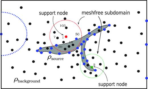
Schematic RBF-FD stencils. A density source, ρ_source, with arbitrary geometry and its background space are discretized by nodes. Here, the black nodes are located inside the background or the source regions; the blue nodes are located on the domain boundary or interfaces. The circles (and the half circles) denote different subdomains for different nodes. RBF-FD stencils can have different number of nodes.

Open in new tab Download slide

Note that [1 x y z] are a complete linear monomial basis in the 3-D space. The method described above can be equally applied to other polynomial enrichments with m > 0 terms of monomial functions, and the local linear system from interpolation will have the dimension of n + m. Also, only w_k, k = 1, 2, ⋅⋅⋅, n, from the solution to eq. (13) are needed and will form the non-zero entries in each row of the matrix when assembling a global matrix equation, with the unknowns as the potential values on all the nodes. Thus, the dimension of the global linear system of equations is equal to the number of nodes, and the coefficient matrix is a sparse, asymmetric matrix. A direct sparse solver (Amestoy et al.2006) is used to solve the global linear system of equations in the following calculations unless otherwise illustrated. Once the global linear system for the potential has been solved, vertical gravity can be directly obtained by taking the gradient of the local interpolant in eq. (8). Similarly, gravity gradients can also be straightforwardly obtained by taking the corresponding second derivatives of the potential interpolant function.

2.5 Boundary conditions in RBF-FD

An important advantage of RBF-based mesh-free interpolation is the straightforward implementation of the essential boundary condition in eq. (3). The RBF-FD approximation of the gravitational potential for nodes at the computational boundaries (Fig. 3) is done in the same way as for other interior nodes. In assembling the global matrix equation, however, we simply set the diagonal entries in rows that correspond to the boundary nodes as a non-zero constant, and all other entries as zero. The remaining rows in the global coefficient matrix all have n non-zero entries.

3 CONVERGENCE OF RBF-FD

3.1 h-convergence

To understand the h-convergence of RBF-FD under global refinement of the cloud of nodes used for discretizing the PDE, we chose a synthetic gravity model for which analytic solutions for both potential and the vertical gravity component g_z are available. The model set-up is identical to that used in Farquharson & Mosher (2009) and May & Knepley (2011), in which a simple prismatic gravity source, with density ρ = 2000 kg m⁻³, is located at the centre of the computational domain and is surrounded by void material with density ρ = 0 kg m⁻³. The dimension of the density source is 100 × 100 × 100 m here. The computational domain is truncated to be Ω = [−500, 500] × [−500, 500] × [−500, 500] m with the length of the cube L = 1000 m in this example. The nodal distribution is uniform but, however, unstructured (Fig. 4). As such, when the internodal distance h decreases, the number of nodes grows as the order of O(N³) with N the estimated number of nodes in each dimension. The truncated domain is not sufficiently large to effectively approximate the boundary condition from eq. (3), and is chosen with the purpose to limit the degrees of freedom under finer nodal refinements so that the problem is solvable on a single workstation computer with 32 GB memory. In this case, analytical potentials (Waldvogel 1976) were used as boundary values. To assess the convergence rate of different RBF-polynomial combinations in the RBF-FD method, the following RMS (root-mean-square) error is computed:

\begin{eqnarray*} \mathrm{ RMS} = \sqrt{ \frac{1}{N} \sum ^{N}_{i=1} \left( \frac{\phi ^{\mathrm{ numer}}_{i} - \phi ^{\mathrm{ exact}}_{i}}{\phi ^{\mathrm{ exact}}_{i}} \right)^2 }, \end{eqnarray*}

(17)

where N is the total number of nodes excluding those on the computational boundaries where the solution is exact, ϕ^numer is the potentials computed by RBF-FD and ϕ^exact the analytical potentials for all interior nodes.

Figure 4.

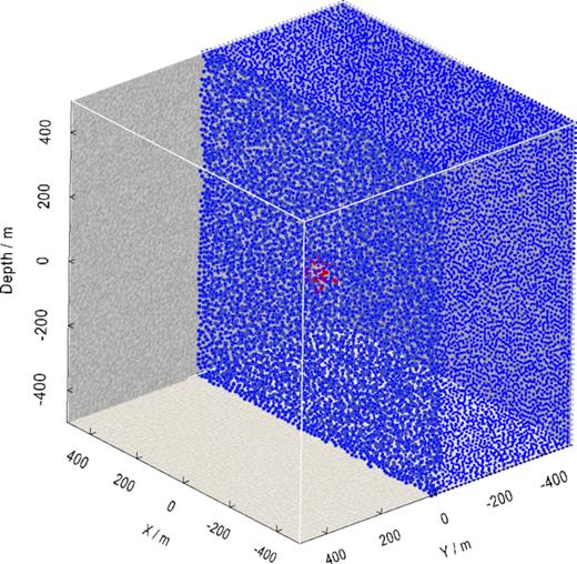
Uniform, unstructured nodes (blue) shown on the surface and at the cross-section y = 0 of the density model for convergence analysis. The red points in the middle of the cross-section are inside the cubic density source.

Open in new tab Download slide

Fig. 5 shows the convergence behaviour for GA and PHS RBF-FDs under refinement. In this test, there are four types of polynomial enrichment: (1) ‘quad’ denotes the complete quadratic polynomial basis functions (note that in 3-D, there are up to four linear polynomial basis functions, and up to 10 quadratic polynomial basis functions, see the RBF-FD theory in the previous section); (2) ‘linear’ denotes the complete linear basis functions; (3) ‘const’ means using only the constant term (f = 1.0); and (4) ‘GA only’ is the GA RBF-FD case without polynomials. For GA RBF-FDs, a fixed shape parameter, which is dimensionless, was used for all nodes in a subdomain. Among different subdomains, this fixed shape parameter c₀ was further scaled by the radius d_i of the smallest sphere enclosing each mesh-free subdomain Ω_i, so that all RBF-FD subdomains have essentially the same flatness of RBFs, and the subdomain Ω_i has the shape parameter

\begin{eqnarray*} c_{i} = \frac{c_{0}}{d_{i}}. \end{eqnarray*}

(18)

The advantage of the method in eq. (18) is that the shape parameter in each subdomain can be automatically determined once the basic c₀ is given. Our tests verified that this is an effective method to choose proper shape parameters in the unstructured nodal arrangements. Here, for GA RBF-FD implementations, c₀ = 0.1 and n = 20, and for PHS-based implementations, k = 5 (i.e. quintic order of r), n = 37, where n is the number of nodes in each subdomain.

Figure 5.

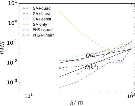
RMS errors of potential versus the averaged internodal distance h. Results of six different RBF-polynomial combinations of RBF-FD are shown as the dashed lines. The two black solid lines indicate the theoretical linear O(h) and quadratic O(h²) convergence rates in the log–log plot.

Open in new tab Download slide

The results in Fig. 5 show a clear h-convergence trend for both types of RBFs except the case of GA-only implementation. However, the divergence of GA-only RBF-FD for finer nodal discretizations is due to the saturation error under refinement that relates to rapidly increasing ill-conditioning of the interpolation linear system (Fornberg et al.2013; Flyer et al.2016a). To overcome the saturation error problem, one can either add additional polynomials to the RBF-based interpolation, as shown in Fig. 5, or use very small shape parameters, which requires a stable computational algorithm to obtain RBF-FD weights. For efficiency, we choose the former method for non-uniform nodal representation with local refinements in later examples. Note that the convergence rate of PHS RBF-FD is more dependent on the highest degree of polynomials enriched, rather on the order of PHS RBFs (Bayona et al.2017). Therefore, high-order h-convergence can be achieved using PHS RBFs enriched with a desired degree of polynomials, although it comes with the cost of slightly more expensive evaluation of RBF-FD weights in eq. (13).

3.2 Influence of GA shape parameter

The choice of c₀ in eq. (18) needs to be made carefully as it affects the overall accuracy of solving the PDEs, especially if the RBF-direct method is adopted. The RBF-direct way was used to solve the interpolation linear systems due to the efficiency concern as discussed in Section 2.3. Although there is no established mathematical analysis so far that provides an error estimate of solving PDEs based on the ill-conditioning of the local interpolation systems, we show here and in the next section, by means of numerical evidence, that the extreme local ill-conditioning, which is resulted from small shape parameter (for infinitely smooth RBFs) and large stencil size, can cause numerical instability in obtaining the interpolation weights, and hence plays a vital role in solving the PDEs. Fig. 6 shows the RMS errors for different c₀ when h = 60 m, which results in 16 638 nodes in total in the model. Correspondingly, Fig. 7 provides the changes of condition number of the local linear system at the node position (x, y, z) = (50.0, 50.0, 50.0), which was chosen just as a representative point of all the nodes. There are three notable c₀ ranges in Fig. 6 that illustrate different behaviours of GA RBF-FD. The first part is c₀ > 0.08 where GA RBFs have very compact support (opposite to the flat limit case), hence the interpolation accuracy is expected to be low, despite that the local approximation is better conditioned than that of small c₀. Correspondingly, relatively high RMS values are observed (Fig. 7). In this case, if enriched by polynomials, the interpolation accuracy is dominated by the highest degree of polynomials, which is reflected in the RMS errors. The second part is when 10⁻⁴ < c₀ < 0.08. In this range, although the conditioning is worse than the first part, the interpolation accuracy is improved (see the RMS for the GA-only case in Fig. 6). This is because our direct evaluation of local linear systems was still correct. Further, the role of enriched polynomials for accuracy becomes less important because as c₀ → 0, the GA RBFs eventually span exactly the same function space as their equivalent-order polynomials do (Flyer et al.2016b). The third part of c₀ range is when c₀ < 10⁻⁴. The local linear systems are becoming so ill-conditioned as c₀ → 0 such that our evaluations of RBF-FD weights using the RBF-direct method become incorrect. As a consequence, the RMS error of the potential solutions also becomes noisy. This is further confirmed by plotting the condition numbers for c₀ < 10⁻⁴ in Fig. 7. The condition numbers were calculated using the same LU factorization method used to obtain the RBF-FD weights, and are expected to linearly increase in the log–log plotting as c₀ decreases (Fasshauer 2007; Fornberg et al.2013), rather than following a nearly flat (wrong) trend as shown in Fig. 7.

Figure 6.

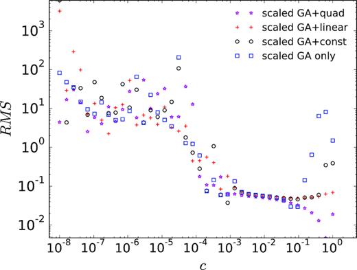
RMS errors of potential versus shape parameter c for GA RBF-FDs with n = 20 nodes in each subdomain. Note that the smaller c is, the flatter the GA RBFs become. Here and for the following, ‘scaled GA’ indicates that all c values shown above correspond to the c₀ in eq. (18).

Open in new tab Download slide

Figure 7.

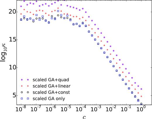
Condition number, κ, of the local linear system for the mesh-free subdomain with support node at (50.0, 50.0, 50.0), for different shape parameter c in GA RBF-FDs. The system has the dimension k × k with k = n + m, where n = 20 is the number of nodes in each subdomain, and m is the number of polynomial terms.

Open in new tab Download slide

It should be noted that the best c range for infinitely smooth RBFs in terms of giving good computational accuracy is also affected by other factors, for example, nodal distribution and type of RBF, and is likely to vary for different problems at hand. This indicates that it would be very difficult to predict a good shape parameter before solving our PDEs. As mentioned earlier, the above ill-conditioning issue can be circumvented by employing stable computing algorithms, instead of direct factorization of the original local linear system matrices. Recently, there have been special attention and efforts devoted to stable evaluation of eq. (13) based on GA RBFs (Fornberg et al.2013) and MQ RBFs (Fornberg & Wright 2004). However, applicability of these algorithms for other RBFs still remains unclear. Furthermore, the time-consuming drawback of this approach also makes it less attractive for practical geophysical data modelling, where the degrees of freedom can be very large. A compromise here is to adopt the RBF-direct method without using too small shape parameter values. For example, Martin et al. (2015) and Li et al. (2017) studied 2-D seismic modelling using MQ RBF and inverse MQ RBFs, respectively, and there they suggest that selecting c values that limit the condition number of the interpolation coefficient matrix to be 10⁶−10⁸ is satisfactory. We note that in RBF-FD, the conditioning of the local coefficient matrix is also sensitive to the number of nodes used to construct mesh-free interpolation (shown in the next section). Therefore, prior empirical experiments are often needed to take other factors into account when using such pre-selected shape parameter values of the infinitely smooth RBFs.

3.3 Influence of stencil size

In our RBF-FDs, the stencil size refers to the number of nodes, n, in each subdomain for a given point discretization, rather than the maximum Euclidean distance among the local nodes. Fig. 8 shows how the RMS error changes with n for the model discretization with h = 60 m. The RMS error reflects the accuracy of the RBF-FD in solving PDEs. The plots here show again that when GA RBFs are used, small c can lead to better numerical accuracy in solving PDEs. Fig. 8 also demonstrates that for the Laplacian opertor, the stencil size n should not be too small for a good RBF-FD solution. In this particular example, it shows that when n < 20 the RMS error starts to deteriorate for both GA and PHS RBFs. On the other hand, increasing n from 30 to 60 does not significantly improve the computational accuracy, suggesting that there is no need to use too many nodes in each RBF-FD subdomain in the 3-D case. These observations of the effects of the stencil size are also echoed in previous numerical studies for 2-D Poisson’s equations (e.g. Bayona et al.2017). In our 3-D tests for different model discretizations, n > 10 for GA RBFs, and n ≥ 3m with m as the number of terms of enriched polynomials (up to quadratic) for PHS RBFs was required to obtain numerical solutions with good accuracies. It should be pointed out that in the PHS RBF-based mesh-free FD implementation, additional polynomials are always recommended as PHS RBFs alone may be only conditionally positive definite functions and can cause singularity issues.

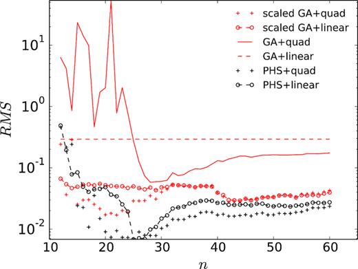
RMS errors of potential versus the RBF-FD stencil size n. For GA RBFs, c0 = 0.3. Here, ‘scaled GA’ indicates that the c0 value is scaled by the radius, di, of the smallest sphere enclosing the subdomain. Note that as a result of the scaling and di > 1, scaled GA RBFs are flatter than the unscaled GA RBFs.

Figure 8.

RMS errors of potential versus the RBF-FD stencil size n. For GA RBFs, c₀ = 0.3. Here, ‘scaled GA’ indicates that the c₀ value is scaled by the radius, d_i, of the smallest sphere enclosing the subdomain. Note that as a result of the scaling and d_i > 1, scaled GA RBFs are flatter than the unscaled GA RBFs.

Open in new tab Download slide

In practice, it is found that as n increases, the condition number of local linear systems also increases approximately linearly. Fig. 9 shows how the condition number of the above local linear system changes with n for the model discretization with h = 60 m. It can also be noted that PHS RBF-based interpolation is generally much more ill-conditioned than GA RBF-based counterpart with modest shape parameter (Fig. 9). This is expected according to the theoretical analysis (e.g. Iske 2003). When using the finite-smoothness RBFs such as PHS, the challenge in stably computing the interpolation coefficients (by solving a possibly very ill-conditioned local linear system) still exists, but now the cause is mainly attributed to the stencil size. Here, we had successful evaluation of RBF-FD weights without problem by just using RBF-direct method for the stencil size n range shown in Fig. 9, despite that the conditioning numbers are mostly more than 10²⁰. For very large condition number situations arising from local refinement, for example, one effective remedy is to scale the local interpolation in eq. (8) by the distance h_s = r₀, with r₀ as the radius of the smallest sphere that encloses all nodes in a subdomain, so that a new subdomain with unit radius is formed. After solving the new linear system, which is shown to be better conditioned by Iske (2003), RBF-FD weights for the original subdomain can be obtained by simply rescaling the calculated interpolation coefficients back by h_s. In addition, using PHS RBFs can completely eliminate the difficulty of finding a suitable shape parameter. For these reasons, the PHS RBF-FD is considered by us to be more computationally efficient than the GA RBF-FD for assembling a global linear system, and is chosen for later modelling examples, unless otherwise illustrated.

Figure 9.

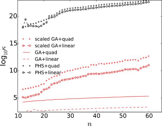
Condition number, κ, of the local linear system for the mesh-free subdomain whose support node is at (50.0, 50.0, 50.0), for different stencil sizes.

Open in new tab Download slide

3.4 Unstructured nodes with local refinements

Unstructured nodal layouts are favoured in our development of mesh-free techniques because they have the most powerful capability of representing highly irregular geometries, which are present in most realistic earth models. The support of local refinements further enables highly efficient computation for 3-D earth models. Several mesh-free studies have been reported for modelling geophysical EM data (Wittke & Tezkan 2014) and seismic wavefield (e.g. Jia & Hu 2006; Martin et al.2015; Takekawa & Mikada 2016; Li et al.2017). However, they are focused on 2-D and use either uniform (i.e. equidistant nodes everywhere), or quasi-uniform (i.e. unstructured but uniform density of nodes), or the combination of these two types of nodal distributions. The drawback of uniform or quasi-uniform nodes for 3-D problems is the computational inefficiency because the degrees of freedom grow as O(N³) with N as the average number of nodes in each dimension. To demonstrate the advantage of non-uniform nodes, the gravitational potential and vertical gravity component were computed for the truncated density model discretized with both quasi-uniform and non-uniform unstructured nodes. The quasi-uniform mesh-free discretization is the same as shown in Fig. 4 with the average internodal distance h = 20 m. However, for the non-uniform case, the boundary of the model is extended to be 500 km such that the homogeneous boundary condition in eq. (3) can be safely used. A line located at −200 m ≤ x ≤ 200 m, y = 0 m, z = 100 m, which is 100 m above the centre of the density source, was designed as the observation sites. The general rule of thumb of local refinement is to refine the regions where better numerical accuracy is desired (e.g. around the measurement sites) and where the unknown function changes most rapidly. For the non-uniform nodal discretization, local refinements were added inside the density source and at the observational sites to improve accuracy (Fig. 10b), which was facilitated by the software Tetgen (Si 2015). The nodal distribution away from the source is much sparser than that of the source. The overall nodal pattern of this distribution is shown in Fig. 10(a).

Figure 10.

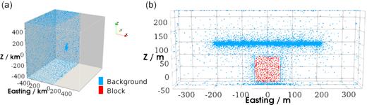
Unstructured, non-uniform nodal discretization displayed in (a) a perspective view of the nodes within the easting −500 km ≤ x ≤ 0 km, and (b) an enlarged view of the local nodal refinements within the blocky density source (the red points, internodal distance h = 10 m) and at the observation sites at the cross-section northing y = 0 m (internodal distance h = 1 m).

Open in new tab Download slide

In this example, the gravitational potential changes more rapidly around the blocky density source than elsewhere. To examine the importance of the local refinement for the density source and the measurement sites, numerical potentials and vertical gravities were calculated at the designed 200 observation sites in the case of (1) local refinement inside the density source and (2) local refinement at the measurement sites. In either case, different scales of local refinements were performed to study the convergence of the RBF-FD under unstructured discretization. The refining scales were controlled manually by requiring different internodal distances in the refinements. Here, the exact potentials and gravities at the measurements were computed by the summation methods of Waldvogel (1976) and Li & Chouteau (1998; by the method of eq. 4), respectively. The relative errors between the computed potentials and gravities by the PHS RBF-FD (enriched by quadratic polynomials) and the exact solutions are plotted in Fig. 11. In the first case, the points around the measurement sites were properly refined (with the internodal distance h = 1 m), and the density source was refined by different scales, as shown in panels (a) and (b) in Fig. 11. In the second case, the density source was properly refined (with h = 10 m), and the points around the measurement sites were refined by different scales, as shown in panels (c) and (d) in Fig. 11. In both cases, the RBF-FD stencil size was fixed as n = 37 to avoid possible adverse effect on accuracy resulted from insufficient number of points in the RBF-FD subdomains. It is shown that in both cases, the numerical solutions converge to the exact solutions under local refinements. Particularly, the local refinement at the measurements improves the smoothness of the numerical solutions. It can also be observed that the density source, or physical property distribution, should be appropriately discretized for accurate modelling. The above observations, although as purely numerical evidence, show that the proposed RBF-FD supports well the local refinement, which is well known in mesh-based methods.

Figure 11.

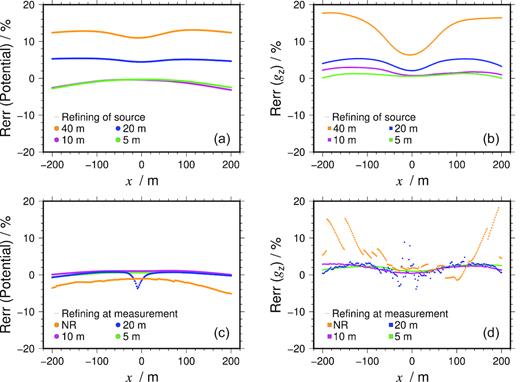
Relative errors for the numerical potential and gravity by RBF-FD along the test line in the blocky density model. Panels (a) and (b) show the errors under different refining scales inside the density source (indicated by the internodal distance h = 40, 20, 10 and 5 m) for potentials and gravities (g_z), respectively. In the case of source refinements, a refinement of h = 1 m was applied at the measurements. Panels (c) and (d) show the corresponding errors under different local refining scales at the measurement sites (indicated by the internodal distance h = 20, 10 and 5 m). The situation without local refinement at the measurements is denoted as NR. In the case of measurement refinements, a refinement of h = 10 m was applied for the density source block.

Open in new tab Download slide

Fig. 12 shows a comparison of the computed potentials and vertical gravities along the x-directed line for the two different nodal layouts with the PHS RBF-FD method: quasi-uniform and unstructured (non-uniform) discretizations. In both situations, PHS RBFs were enriched with quadratic polynomials. In the case of quasi-uniform nodes, RBF-FD stencil size n = 30. While for the non-uniform case, n = 37. Also, local refinements with h = 9.5 m for the density source and h = 1 m for the measurement sites were applied for the unstructured discretization. The computed potentials and gravities for these two different model discretizations agree well with analytic potentials (Waldvogel 1976) and vertical gravities (by the method of eq. 4 in Li & Chouteau 1998), respectively. While the quasi-uniform discretization required 367 605 nodes, the non-uniform discretization only had 72 082 nodes, which is approximately one-fifth of the former number. It is worth noting that the latter model also has much larger computational domain, which supports practical boundary condition that assumes little about the density source. In our experiments, the refining scale, for example, the smallest nodal distance in refined regions, played a more important role than RBF-FD stencil size n in obtaining accurate numerical results. To maximally benefit from local refinements, adaptive refining strategies would be more practical. However, this is currently not covered in this study and will be addressed in another research work.

Figure 12.

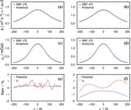
Computed potential (ϕ), vertical gravity (g_z) and their relative errors (Rerr) by the PHS RBF-FD for the quasi-uniform nodes with the averaged internodal distance h = 20 m (panels a, c and e), and for the non-uniform, unstructured node discretization discussed in the text (panels b, d and f).

Open in new tab Download slide

The gravity gradient tensor components (U_xx, U_xy, U_xz, U_yy, U_yz and U_zz) were also computed using the same above settings of the PHS RBF-FD with the non-uniform node discretization, and are shown in Fig. 13. The results are for the same observation line as in Fig. 12, which mimics an airborne gravity gradiometry measurement. Although U_zz is often not considered an independent component of the gradient tensor, it was calculated independently (i.e. not using U_xx and U_yy) and is included here for completeness. It can be observed that the numerical results of gradients have an excellent agreement with the analytical results, which were computed by the summation method of Okabe (1979).

Figure 13.

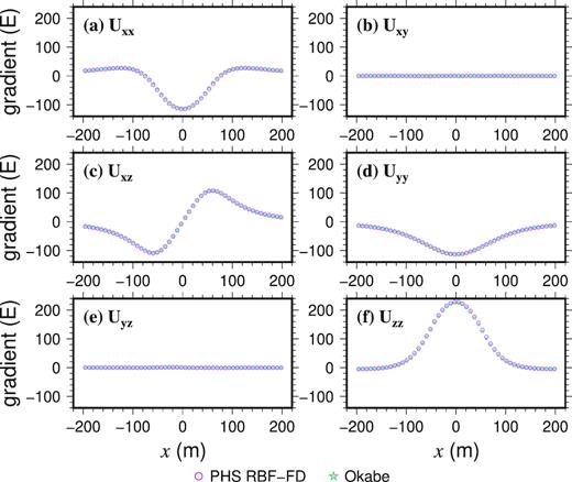
Comparison of six components of gravity gradient tensor (U_xx, U_xy, U_xz, U_yy, U_yz and U_zz) calculated using the PHS RBF-FD method with the non-uniform, unstructured node discretization, and using a summation method (Okabe 1979). The gradient values are shown in Eotvos (E).

Open in new tab Download slide

4 COMPARISON WITH FINITE-ELEMENT METHOD

In this section, we show comparison studies between nodal FE and RBF-FD mesh-free methods with an irregular density model. The density model built here is a reconstruction of part of the Bay du Nord reservoir located at the Flemish Pass Basin offshore eastern Canada (Dunham et al.2018). The model has two non-zero density blocks: one is the reservoir unit with maximal thickness of 100 m and the other is a Cretaceous sedimentary layer with an averaged thickness of 300 m. The reservoir unit is overlain by and truncated at one end by the sedimentary unit, see Fig. 14. The rest of the model is filled with void region with zero density. Although the geometries of the reservoir and overlying unit are not very extreme, the curved surface of the attachment of the two units forms a wedge-like sharp angle, which becomes a challenge for the meshing process in the FE method (Fig. 16). Fig. 15 shows the cross-section in the y−z plane of the model at the easting x = 0 m. Two vertical lines, also shown in the section view in Fig. 15, represent measurement sites for which the mesh-free and FE solutions are tested. The range of vertical coordinates of both lines is from z = −2.5 km to z = −4.0 km. The northing (y) coordinates are y₁ = −3.5 km and y₂ = −1.0 km, respectively. The Cretaceous sedimentary layer has a uniform density ρ₁ = 2200 kg m⁻³, while the reservoir is assigned the density ρ₂ = 2600 kg m⁻³.

Figure 14.

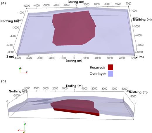
Perspective 3-D views of the Bay du Nord density model. The easting is along the x-direction, and the northing is along the y-direction. Panel (a) shows the reservoir unit overlain by the sedimentary unit. The view is looking from south to north. Panel (b) is a side view from north to south. A 2-D cross-section at x = 0 (easting) that cuts through the two plates is given in Fig. 15.

Open in new tab Download slide

Figure 15.

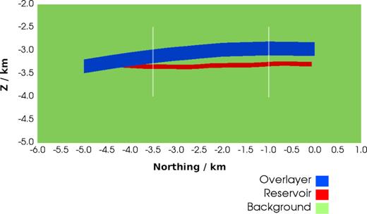
Vertical cross-section of the Bay du Nord model at x = 0 (easting, looking from the positive x-direction). The northing direction is along the y-axis. Two vertical white lines mark the positions of two lines at y₁ = −3.5 km and y₂ = −1.0 km.

Open in new tab Download slide

4.1 Discretization

To enforce the boundary condition in eq. (3), the computational domain is set to be −50 km ≤ x ≤ 50 km, −50 km ≤ y ≤ 50 km, −50 km ≤ z ≤ 50 km, with 100 km length of each side of the cubic box. For both FE and RBF-FD methods, unstructured discretizations are employed to honour the irregular geometries. In the FE case, tetrahedralized meshes were constructed using the open source software Tetgen (Si 2015). For the mesh-free discretization, the nodes generated as vertices of the tetrahedral elements of the mesh for FE computation have been adopted, despite that completely different ways of generating nodes can be used. We used the same set of nodes here in the test so that the numerical performances from FE and mesh-free codes can be compared with as minimal discrepancies from the model discretization as possible. In this case, the linear systems from the node-based FE and RBF-FD methods will have exactly the same dimension and the same unknowns. As before, local refinements were carried out near the measurement sites and within the reservoir and overlayer blocks. A comparison of the meshed and node-based discretizations is depicted in Fig. 16.

Figure 16.

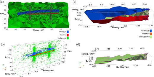
Unstructured mesh (panel a) and mesh-free nodes (panel b) for the section shown in Fig. 15. Note that the mesh is located on the 3-D crinkled surface at easting x = 0 m, and the nodes in panel (b) are 3-D nodes within the cubic domain: −0.75 km < x < 0.75 km, −6.0 km < y < 1.0 km, −5.0 km < z < −2.0 km. Panel (c) shows the enlarged 3-D view of the mesh around the wedge-like adjoint that is shown in panel (a). Panel (d) shows the same enlarged view as in panel (c) but only with the tetrahedral elements in the background region. In panel (d), the tetrahedra shown at the southern end become increasingly thin wedge- or sliver-like elements.

Open in new tab Download slide

4.2 Numerical accuracy

The accuracy of the numerical results is assessed by comparing them against the analytical solution based on the method described in Okabe (1979), in which the vertical gravity response at a specific position is obtained by summing up the calculation over each tetrahedron from the mesh. The FE results of the gravity were computed by assuming that linear basis functions are used for both test and trial functions to derive a weak form solution to the potential of eq. (1), for which implementation details are presented in Jahandari & Farquharson (2013). Three different tetrahedralizations were generated here using increasingly higher quality controls, but without changing the local refinement constraints. The model discretizations are represented by the total node number as N = 62 418, 73 047 and 83 948, respectively. Also, the total element number is N_ele = 392 363, 459 129 and 526 796, respectively. The node number is also the matrix dimension of the linear system resulted from assembling local interpolation coefficients either by the FE or mesh-free approximation. In this example, the local subdomain size of the RBF-FD mesh-free method is set to be n = 30, while in the FE case the support of basis function, therefore, n, depends on the mesh topology. Because of the difference in the number of points used for local linear system of interpolations between FE and RBF-FD methods, the assembled global linear systems of the two schemes will have different number of non-zeroes. The numerical results of vertical gravities, g_z, are plotted in Fig. 17. The results show that both numerical methods converge to the true solution as N increases. It is also observed that for N = 62 418 the RBF-FD result is less accurate than that of FE method. However, the accuracy situation is reversed for the case when N = 83 948. Particularly, the RBF-FD solution accurately captures the sudden changes of g_z around the sharp density discontinuities where g_z is not smooth, whereas the FE solution appears to be struggling for this.

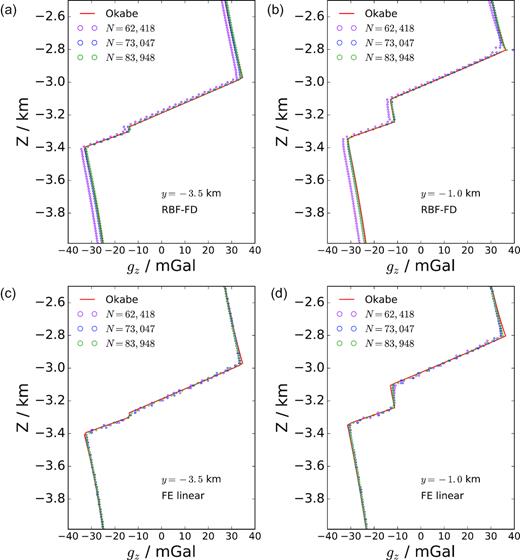
Calculated gz along two vertical lines, y1 = −3.5 km and y2 = −1.0 km, for three different model discretizations (the total number of nodes, indicated by N) with RBF-FD (panels a and b) and linear FE (panels c and d) methods. Analytical solutions are denoted by ‘Okabe’.

Figure 17.

Calculated g_z along two vertical lines, y₁ = −3.5 km and y₂ = −1.0 km, for three different model discretizations (the total number of nodes, indicated by N) with RBF-FD (panels a and b) and linear FE (panels c and d) methods. Analytical solutions are denoted by ‘Okabe’.

Open in new tab Download slide

As shown previously, RBF-FD solution can also be affected by the stencil size for a given model discretization. Often a sufficient number of nodes, n, is required for accurate modelling. In general, n can be different from one subdomain to another. For the purpose of easy implementation, we have used a fixed number of nodes over all mesh-free subdomains. The numerical accuracies of using different n values in the PHS RBF-FD method are shown in Fig. 18. In this example, the total number of nodes was N = 62 418. By increasing n from 30 to 50, there is a clear overall error reduction of g_z for both lines. Fig. 18 also illustrates that the largest errors arise near the large density contrasts of the region and are persistent as n increases. By recalling previous results from Fig. 17, it is suggested that refinement is more important than increasing stencil size to reduce errors in the contacts of different physical property values, or in regions where high gradients in the unknown function are expected.

Figure 18.

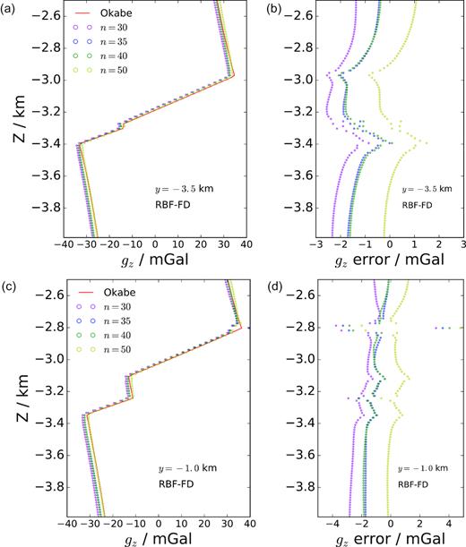
Calculated g_z along two vertical lines by RBF-FD method with different stencil sizes, n = 30, 35, 40 and 50. The errors shown in the right-hand panels (b and d) are the subtraction between the RBF-FD solution and analytical solution.

Open in new tab Download slide

For computational efficiency, the RBF-FD methods implemented here are generally slower than the linear FE counterparts in assembling and solving the system of equations. The main reason lies in the necessity of numerically evaluating the local linear equations from eq. (13) for RBF-FD methods. Also, due to the fixed RBF-FD stencil size, the PHS RBF-FD is likely to generate more non-zero entries than the linear FE method. For example, when N = 73 047 in which the RBF-FD and the linear FE gave comparably the same accuracy, and the stencil size was n = 30, the number of non-zero entries in the RBF-FD linear system was nnz = 2187 814, while in the linear FE case nnz = 1137 641. The computational time in seconds for the mesh-free case was 33.410 s (28.407 s for assembling, and 5.003 s for solving the linear system), while the same computational time for the latter was 18.624 s (14.427 s for assembling, and 4.197 s for solving the linear system). For the post-processing time (i.e. the time amount needed to obtain vertical gravities from potentials after solving the linear system) with 200 measurement sites here, the RBF-FD used only about 0.1 s due to the use of k-dimensional tree structures, while the linear FE required 3.172 s due to necessary geometry searching calculations (e.g. finding which elements a chosen node or measurement site belong to in the unstructured mesh) in a standard FE implementation. It is worth noting that the geometry searching calculation is also typically needed prior to the assembling of the linear system in the FE scenario, which, depending on the algorithm, may require additional non-negligible computational time.

4.3 Conditioning of the global differential matrix

Conditioning of the coefficient matrix of the global linear system resulted from PDE-solving methods can largely affect the convergence of solving the system if an iterative solver is used. The FE coefficient matrix |$\mathbf {M}_{\mathrm{ FE}}$| is symmetric, although the matrix can be very ill-conditioned due to unstructured meshes and local refinement. In the RBF-FD method, however, the counterpart matrix |$\mathbf {M}_{\mathrm{ RBF}}$| is non-symmetric, indicating that some complex eigenvalues will exist. Fig. 19 shows the distributions of eigenvalues of |$\mathbf {M}_{\mathrm{ FE}}$| and |$\mathbf {M}_{\mathrm{ RBF}}$| in the complex plane, with linear systems assembled from the Bay du Nord model discretization with N = 41 711. All eigenvalues of |$\mathbf {M}_{\mathrm{ FE}}$| are real-valued numbers here. In the linear FE case, eigenvalues only have one cluster, although they are distributed over a large range of values and the ratio of the largest eigenvalue (1.55e + 13) and the smallest eigenvalue (3.77e + 2) is large. On the other hand, |$\mathbf {M}_{\mathrm{ RBF}}$| has a much tighter cluster of eigenvalues along the real axis. However, the eigenvalue distribution of |$\mathbf {M}_{\mathrm{ RBF}}$| has two symmetric outliers in the complex plane, which would make the convergence of iterative solvers difficult. Our tests using generalized minimal residual (GMRES; Saad & Schultz 1986) with incomplete LU factorization as pre-conditioner confirmed that the convergence of solving RBF-FD generated system is much slower than that of solving FE problem for this example.

Figure 19.

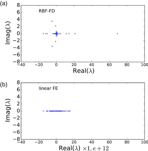
Distribution of eigenvalues, λ, of RBF-FD and FE coefficient matrices in the complex plane for the Bay du Nord model.

Open in new tab Download slide

5 OVOID ORE DEPOSIT MODEL—A REALISTIC EXAMPLE

The realistic density model here represents the Voisey’s Bay massive sulfide deposit located in Labrador, Canada. Fig. 20 shows the irregular geometries of the deposit. Prior to the geophysical study, the surface structure of the deposit was roughly triangulated, as can be seen in Fig. 20, when building up the geological model. To forward model the borehole vertical gravity and airborne gravity tensor components for this model, the deposit is assigned a constant density ρ = 2000 kg m⁻³ and is surrounded by void material (i.e. the background density ρ_b = 0 kg m⁻³) in this example. The model set-up is identical to the same Ovoid deposit example by Jahandari & Farquharson (2013). An example of the mesh-free nodal discretization is given in Fig. 21. The computational domain is extended to be −500 km ≤ x ≤ 500 km, −500 km ≤ y ≤ 500 km and −500 km ≤ z ≤ 500 km with the deposit at the central part, so that the boundary condition in eq. (3) is valid.

Figure 20.

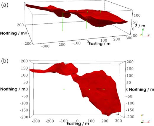
3-D perspective views of the Ovoid ore deposit. Panel (a) shows a 3-D view of the deposit with three vertical lines (shown in the solid green), which mimic the borehole measurement sites. Panel (b) shows a view of the ore deposit, looking from the positive z-direction, with the three green dots indicating the locations of vertical lines.

Open in new tab Download slide

Figure 21.

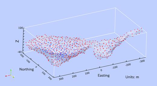
An example of nodal discretization of the Ovoid ore deposit. Nodes located at the deposit’s surface are shown in red, and the interior nodes are shown in blue.

Open in new tab Download slide

Three vertical lines mimicking borehole gravity measurements and one horizontal line for the airborne gravity gradients are designed here to verify our mesh-free solutions. The four lines are graphically depicted in Figs 20 and 22. They are all located in the cross-section with zero northing (y = 0; see Fig. 22). For the vertical lines, they have the easting x₁ = 200 m (line 1), x₂ = 90 m (line 2) and x₃ = −100 m (line 3), respectively, and have the same z coordinates from 80 to −60 m. Line 1 has most of its measurement sites located within the deposit, while line 3 is completely outside the deposit. Line 2 cuts part of the deposit in the west end and interacts with the deposit’s surface in about 90 deg at the top and sloping 45 deg at the bottom. The horizontal profile (line 4) extends from easting x = −300 m to x = 300 m, with z = 200 m, which is approximately 120 m above the highest point of the deposit.

Figure 22.

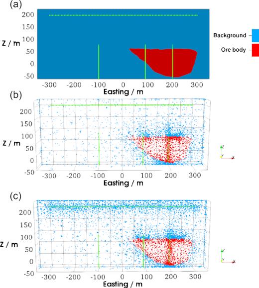
Comparison of the nodal discretizations shown for the 2-D cross-section at northing y = 0. Panel (a) shows the 2-D section with three vertical lines (the solid green) and one horizontal line (the dotted green). Panel (b) shows the nodal pattern for a mesh-free discretization with refinements only along the vertical line at easting x = 200 m and inside the ore deposit. Panel (c) shows the pattern for another mesh-free discretization, which, compared to that in panel (b), has additional nodal refinements along the horizontal line.

Open in new tab Download slide

The first mesh-free discretization for the computational domain comprises 76 990 nodes in total. In this example, nodal discretization inside the deposit was refined by setting the averaged internodal distance h = 50 m. In addition, line 1 was refined with the nodal distance h ≥ 5 m. Nodes outside the deposit become gradually sparser towards the boundary. We remark that the refinement inside the density source ensures that the density distribution can be appropriately sampled by nodes in the RBF-FD, while the further refinement for the line 1 at x = 200 m improves local numerical solutions of gravity at those observations. Since the line 3 is outside the density source, gravity changes along this line are expected to be smoother than those of line 1 and 2. Similarly, it can also be expected that line 2 has smoother vertical gravities than that of line 1. As a consequence, extra local refinement is less important at these locations and was not carried out. A visual depiction of the nodal distribution for the y = 0 section is given in panel (b) in Fig. 22. The accuracy for this mesh-free discretization is verified by the computed results of g_z plotted in Fig. 23. The mesh-free results agree well with those calculated using an analytical method, for the three borehole lines. Here, the mesh-free solution was obtained by the PHS RBF-FD with stencil size n = 30 and quadratic polynomials, and the analytical solution was computed using the summation-based method from Okabe (1979). In the latter scenario, the deposit was again tetrahedralized before applying the summation algorithm to each tetrahedron.

Computed vertical gravities, gz, along the three vertical lines with x1 = 200 m, x2 = 90 m and x2 = −100 m that are shown in Fig. 22 using the mesh-free RBF-FD of this study and a summation-based method (Okabe 1979).

Figure 23.

Computed vertical gravities, g_z, along the three vertical lines with x₁ = 200 m, x₂ = 90 m and x₂ = −100 m that are shown in Fig. 22 using the mesh-free RBF-FD of this study and a summation-based method (Okabe 1979).

Open in new tab Download slide

To test the ability of the mesh-free method to obtain accurate gravity gradients, the six components (U_xx, U_xy, U_xz, U_yy, U_yz and U_zz) of the gradient tensor were again computed using the same PHS RBF-FD settings that were used for computing g_z at borehole measurements. In this scenario, a finer nodal discretization was created to study the difference in numerical solutions caused by the nodal density. The finer nodal discretization differs from the first one in that an extra refinement with h ≥ 5 m was applied to the line 4, which is the observation profile. This gives the total node number as 81 135. The difference in the two discretizations is shown in Fig. 22. The computed gravity gradients for both discretizations are plotted in Fig. 24. A surprising observation is that the gravity gradients computed using the coarse discretization already exhibit a reasonably good agreement with the analytical solution Okabe (1979), though with small fluctuations. The obtained gravity gradients using the finer discretization have an excellent agreement with the analytical solution. Such agreement of the gradients would require at least second-order basis functions be used if using FE techniques.

Figure 24.

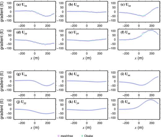
Comparison of computed gravity gradient components (U_xx, U_xy, U_xz, U_yy, U_yz and U_zz) for the horizontal line with −300 m ≤ x ≤ 300 m, y = 0 m and z = 200 m, which is shown in Fig. 22, using the mesh-free RBF-FD of this study and a summation-based method (Okabe 1979). Panels (a)–(f) show the mesh-free results using the nodal discretization without refinements along the horizontal line, while panels (g)–(l) show the mesh-free results using the discretization with refinements for the horizontal line. All gradient values are in the unit of Eotvos (E).

Open in new tab Download slide

6 CONCLUSIONS AND DISCUSSION

A mesh-free method based on the strong form of PDEs and using a new type of RBFs is proposed to forward model gravity data and gravity gradient by solving the boundary value problem for the gravity potential. The purpose is to develop an alternative method different from traditional mesh-based modelling methods such as FE and FV in the PDE-solving category. The main advantage of the mesh-free methods over mesh-based ones is that creation and manipulation of 3-D meshes in the context of forward modelling and inversion can be eliminated, which can be particularly beneficial for earth models with complicated interfaces and/or topographies. The mesh-free method investigated here, mostly called RBF-FD in the literature, has proven successful in accurately modelling gravity responses over complex density models. For the efficiency, although the mesh-free implementation here is shown to be slower in assembling the linear system when compared to the traditional FE method, the overall modelling time of the former could be well less than the latter if one takes into account the efforts in preparing a good mesh and possible geometry search calculations related to the mesh.

In RBF-FD, different RBF functions can be used for mesh-free interpolation. It is shown that the infinitely smooth type of RBFs faces the dilemma caused by choosing an appropriate shape parameter in the application of solving PDEs. In contrast, finite-smoothness RBFs such as PHSs do not have such a problem. When using the infinitely smooth RBFs, one can obtain good numerical results by carefully choosing a proper shape parameter associated with the RBF itself if a direct solving of the resulting small linear system (i.e. without transformation of the original matrix by changing basis or other means) is preferred. However, when using PHS RBFs, which belong to the type of finite-smoothness RBFs, such selection of a good shape parameter can be entirely avoided. We conclude that the RBF-FD based on the finite-smoothness RBFs is more computationally efficient than that based on the infinitely smooth RBFs since in the former situation, no extra computational cost, for example, the costs of determining a good shape parameter and of improving the conditioning, is introduced, and little assumption on the unknown function is made in the evaluation of the local interpolation problem. When using PHS RBFs, it is recommended some polynomial functions are always enriched in the interpolation. Using PHS RBFs enriched with quadratic polynomials, it is shown that RBF-FD can effectively solve the Poisson’s equation of gravity. Like FE and FV techniques, the linear systems generated by RBF-FD are sparse, and local refinements are easily supported to improve accuracies in regions of interest. Our numerical tests show that for both GA and PHS RBFs, the RBF-FD stencil size should not be too small. For 3-D PHS RBFs enriched with low-order polynomials, the stencil size n ≥ 3m, with m the number of terms of enriched polynomials, gives good numerical results. Further, the RBF-FD method can have nonlinear convergence under nodal refinements if enriched with nonlinear polynomials.

We have demonstrated numerically that unstructured nodes with local refinements work well for the presented RBF-FD method. The success of this combination suggests that the presented mesh-free technique can deal with the forward modelling for large-scale earth models. Although uniform (structured or unstructured) nodes are relatively easy to generate in mesh-free techniques, we recommend non-uniform, unstructured nodes be used for the 3-D modelling problems since in the former scenario, the degrees of freedom for a practical 3-D geophysical earth model can readily become untractable. For both synthetic and realistic density models with irregular geometries, the local refinement of nodes around the measurement sites and in regions where the gradient of the gravitational potential changes rapidly, enabled accurate modelling of the vertical gravity data.

For the sake of simplicity of implementation, we chose to use a fixed stencil size for every RBF-FD subdomain here. An open question is, can one use variable RBF-FD stencil sizes while maintaining the same accuracy and efficiency? There have been suggestions (e.g. Wright & Fornberg 2006) that the use of variable stencil sizes, with the points appropriately selected in each subdomain, could potentially improve the accuracy. However, the formation of such varying stencil sizes for non-uniform mesh-free discretizations requires some sort of intelligent search algorithm to select desired stencils, which can be expensive in computation. In this case, a related problem is the effect of the distribution quality of the points in the subdomains on the solution accuracy. Here, the quality of the local points varies from subdomain to subdomain due to the unstructured discretization. A further investigation of using varying stencil sizes would be interesting.

One unsolved issue here is the observed slow convergence of the tested iterative solver, that is GMRES, compared to the standard nodal FE method, for the RBF-FD linear systems. However, the issue itself is closely related to an appropriate choice of the pre-conditioner. Our initial investigation here showed that the slow convergence of the GMRES method with incomplete LU decomposition as the pre-conditioner is likely caused by the scattered distribution of eigenvalues of the coefficient matrix. Because of the nature of our current mesh-free approximation over subdomains, the resultant linear system of RBF-FD is inevitably non-symmetric. Further investigations on the efficient iterative solvers for the RBF-FD method will be a next step.

ACKNOWLEDGEMENTS

JL acknowledges the financial support of a PhD scholarship from Chinese Scholarship Council (CSC), China, and School of Graduate Studies (SGS) from Memorial University of Newfoundland, Canada. Hormoz Jahandari is thanked for valuable suggestions on using the FE code and on generating meshes for the Bay du Nord model in this study. Michael Dunham is also thanked for providing initial frame data for us to build up the Bay du Nord model. JL would also like to thank Scott MacLachlan for discussions about ill conditioning of general matrices, and Peter Lelièvre for using his code implementation in computing the gravity gradients in this study. We thank the editor Juan Carlos Afonso and the reviewers (Jan Wittke and three anonymous others) for their constructive comments that improved the manuscript.

REFERENCES

Amestoy

P.R.

,

Guermouche

A.

,

LExcellent

J.-Y.

,

Pralet

S.

,

2006

.

Hybrid scheduling for the parallel solution of linear systems

,

Parallel Comput.

,

32

(

2

),

136

–

156

..

10.1016/j.parco.2005.07.004

Anderson

E.

et al. .,

1999

.

LAPACK Users’ Guide, Society for Industrial and Applied Mathematics

, 3rd edn,

Society for Industrial and Applied Mathematics

.

Google Scholar

Google Preview

OpenURL Placeholder Text

WorldCat

Ansari

S.

,

Farquharson

C.G.

,

2014

.

3-D finite-element forward modeling of electromagnetic data using vector and scalar potentials and unstructured grids

,

Geophysics

,

79

(

4

),

E149

–

E165

.

Atluri

S.N.

,

Shen

S.

,

2002

.

The Meshless Local Petrov-Galerkin (MLPG) method: a simple & less-costly alternative to the finite element and boundary element methods

,

Comput. Model. Eng. Sci.

,

3

(

1

),

11

–

51

.

Google Scholar

OpenURL Placeholder Text

WorldCat

Banerjee

B.

,

Das Gupta

S.

,

1977

.

Gravitational attraction of a rectangular parallelepiped

,

Geophysics

,

42

(

5

),

1053

–

1055

..

Barbosa

V.C.F.

,

Silva

J.B.

,

Medeiros

W.E.

,

1997

.

Gravity inversion of basement relief using approximate equality constraints on depths

,

Geophysics

,

62

(

6

),

1745

–

1757

..

Barnett

C.

,

1976

.

Theoretical modeling of the magnetic and gravitational fields of an arbitrarily shaped three-dimensional body

,

Geophysics

,

41

(

6

),

1353

–

1364

..

Bayona

V.

,

Flyer

N.

,

Fornberg

B.

,

Barnett

G.A.

,

2017

.

On the role of polynomials in RBF-FD approximations: II. Numerical solution of elliptic PDEs

,

J. Comput. Phys.

,

332

,

257

–

273

..

10.1016/j.jcp.2016.12.008

Bear

G.W.

,

Al-Shukri

H.J.

,

Rudman

A.J.

,

1995

.

Linear inversion of gravity data for 3-D density distributions

,

Geophysics

,

60

(

5

),

1354

–

1364

..

Belytschko

T.

,

Lu

Y.Y.

,

Gu

L.

,

1994

.

Element-free Galerkin methods

,

Int. J. Numer. Methods Eng.

,

37

,

229

–

256

..

10.1002/nme.1620370205

Blakely

R.J.

,

1996

.

Potential Theory in Gravity and Magnetic Applications

,

Cambridge Univ. Press

.

Google Scholar

Google Preview

OpenURL Placeholder Text

WorldCat

Buhmann

M.D.

,

2003

,

Radial Basis Functions

,

Cambridge Univ. Press

.

Cai

Y.

,

Wang

C.-y.

,

2005

.

Fast finite-element calculation of gravity anomaly in complex geological regions

,

Geophys. J. Int.

,

162

(

3

),

696

–

708

..

10.1111/j.1365-246X.2005.02711.x

Chasseriau

P.

,

Chouteau

M.

,

2003

.

3-D gravity inversion using a model of parameter covariance

,

J. Appl. Geophys.

,

52

(

1

),

59

–

74

..

10.1016/S0926-9851(02)00240-9

Chen

J.-S.

,

Hillman

M.

,

Chi

S.-W.

,

2017

.

Mesh-free methods: progress made after 20 years

,

J. Eng. Mech.

,

143

(

4

),

1

–

38

.

Davis

K.

,

Li

Y.

,

2011

.

Fast solution of geophysical inversion using adaptive mesh, space-filling curves and wavelet compression

,

Geophys. J. Int.

,

185

(

1

),

157

–

166

..

10.1111/j.1365-246X.2011.04929.x

Davydov

O.

,

Oanh

D.T.

,

2011

.

On the optimal shape parameter for Gaussian radial basis function finite difference approximation of the Poisson equation

,

Comput. Math. Appl.

,

62

(

5

),

2143

–

2161

.

Du

Q.

,

Gunzburger

M.

,

Ju

L.

,

2002

.

Mesh-free, probabilistic determination of point sets and support regions for meshless computing

,

Comput. Methods Appl. Mech. Eng.

,

191

(

13-14

),

1349

–

1366

..

10.1016/S0045-7825(01)00327-9

Du

Q.

,

Wang

D.

,

Zhu

L.

,

2009

.

On mesh geometry and stiffness matrix conditioning for general finite element spaces

,

SIAM J. Numer. Anal.

,

47

(

2

),

1421

–

1444

..

Dunham

M.W.

,

Ansari

S.

,

Farquharson

C.G.

,

2018

.

Application of 3-D marine controlled-source electromagnetic finite-element forward modeling to hydrocarbon exploration in the Flemish Pass Basin offshore Newfoundland, Canada

,

Geophysics

,

83

(

2

),

WB33

–

WB49

.

D'Urso

M.G.

,

2014a

.

Analytical computation of gravity effects for polyhedral bodies

,

J. Geod.

,

88

(

1

),

13

–

29

..

10.1007/s00190-013-0664-x

D'Urso

M.G.

,

2014b

.

Gravity effects of polyhedral bodies with linearly varying density

,

Celest. Mech. Dyn. Astron.

,

120

(

4

),

349

–

372

..

10.1007/s10569-014-9578-z

Farquharson

C.G.

,

2008

.

Constructing piecewise-constant models in multidimensional minimum-structure inversions

,

Geophysics

,

73

(

1

),

K1

–

K9

.

Farquharson

C.G.

,

Mosher

C.R.W.

,

2009

.

Three-dimensional modelling of gravity data using finite differences

,

J. Appl. Geophys.

,

68

(

3

),

417

–

422

..

10.1016/j.jappgeo.2009.03.007

Fasshauer

G.E.

,

2007

.

Mesh-free Approximation Methods with Matlab

, Vol. 6,

World Scientific

.

Google Scholar

Google Preview

OpenURL Placeholder Text

WorldCat

Fasshauer

G.E.

,

McCourt

M.J.

,

2012

.

Stable evaluation of Gaussian radial basis function interpolants

,

SIAM J. Sci. Comput.

,

34

(

2

),

A737

–

A762

.

Fasshauer

G.E.

,

Zhang

J.G.

,

2007

.

On choosing ‘optimal’ shape parameters for RBF approximation

,

Numer. Algorithms

,

45

(

1-4

),

345

–

368

..

10.1007/s11075-007-9072-8

Flyer

N.

,

Wright

G.B.

,

Fornberg

B.

,

2014

.

Radial basis function-generated finite differences: a mesh-free method for computational geosciences

,

OpenURL Placeholder Text

WorldCat

. .

,

Freeden

W.

,

Nashed

M.Z.

,

Sonar

T.

in

Handbook of Geomathematics

, Vol.

130

,

Springer

, pp.

2635

–

2669

.

Google Scholar

Google Preview

OpenURL Placeholder Text

WorldCat

Flyer

N.

,

Barnett

G.A.

,

Wicker

L.J.

,

2016a

.

Enhancing finite differences with radial basis functions: experiments on the Navier–Stokes equations

,

J. Comput. Phys.

,

316

,

39

–

62

..

10.1016/j.jcp.2016.02.078

Flyer

N.

,

Fornberg

B.

,

Bayona

V.

,

Barnett

G.A.

,

2016b

.

On the role of polynomials in RBF-FD approximations: I. Interpolation and accuracy

,

J. Comput. Phys.

,

321

,

21

–

38

..

10.1016/j.jcp.2016.05.026

Fornberg

B.

,

Flyer

N.

,

2015a

.

Solving PDEs with radial basis functions

,

Acta Numer.

,

24

,

215

–

258

..

10.1017/S0962492914000130

Fornberg

B.

,

Flyer

N.

,

2015b

.

Fast generation of 2-D node distributions for mesh-free PDE discretizations

,

Comput. Math. Appl.

,

69

(

7

),

531

–

544

..

10.1016/j.camwa.2015.01.009

Fornberg

B.

,

Piret

C.

,

2007

.

A stable algorithm for flat radial basis functions on a sphere

,

SIAM J. Sci. Comput.

,

30

(

1

),

60

–

80

.

Fornberg

B.

,

Wright

G.

,

2004

.

Stable computation of multiquadric interpolants for all values of the shape parameter

,

Comput. Math. Appl.

,

48

(

5-6

),

853

–

867

.

Fornberg

B.

,

Driscoll

T.A.

,

Wright

G.

,

Charles

R.

,

2002

.

Observations on the behavior of radial basis function approximations near boundaries

,

Comput. Math. Appl.

,

43

(

3-5

),

473

–

490

..

10.1016/S0898-1221(01)00299-1

Fornberg

B.

,

Larsson

E.

,

Flyer

N.

,

2011

.

Stable computations with Gaussian radial basis functions

,

SIAM J. Sci. Comput.

,

33

(

2

),

869

–

892

..

Fornberg

B.

,

Lehto

E.

,

Powell

C.

,

2013

.

Stable calculation of Gaussian-based RBF-FD stencils

,

Comput. Math. Appl.

,

65

(

4

),

627

–

637

.

Gross

L.

,

Altinay

C.

,

Shaw

S.

,

2015

.

Inversion of potential field data using the finite element method on parallel computers

,

Comput. Geosci.

,

84

,

61

–

71

..

10.1016/j.cageo.2015.08.011

Guillen

A.

,

Menichetti

V.

,

1984

.

Gravity and magnetic inversion with minimization of a specific functional

,

Geophysics

,

49

(

8

),

1354

–

1360

..

Günther

T.

,

Rücker

C.

,

Spitzer

K.

,

2006

.

Three-dimensional modelling and inversion of DC resistivity data incorporating topography-II. Inversion

,

Geophys. J. Int.

,

166

(

2

),

506

–

517

.

Guzman

S.

,

2015

.

Forward modeling and inversion of potential field data using partial differential equations, Ph.D. thesis

,

Colorado School of Mines

.

Haber

E.

,

Holtham

E.

,

Davis

K.

,

2014

.

Large-scale inversion of gravity gradiometry with differential equations

, in

SEG Technical Program Expanded Abstracts 2014

, pp.

1302

–

1307

.,

Society of Exploration Geophysicists

.

Google Scholar

Google Preview

OpenURL Placeholder Text

WorldCat

Hansen

R.

,

1999

.

An analytical expression for the gravity field of a polyhedral body with linearly varying density

,

Geophysics

,

64

(

1

),

75

–

77

.

Hardy

R.L.

,

1971

.

Multiquadric equations of topography and other irregular surfaces

,

J. geophys. Res.

,

76

(

8

),

1905

–

1915

..

10.1029/JB076i008p01905

Holstein

H.

,

2002

.

Gravimagnetic similarity in anomaly formulas for uniform polyhedra

,

Geophysics

,

67

(

4

),

1126

–

1133

..

Holstein

H.

,

2003

.

Gravimagnetic anomaly formulas for polyhedra of spatially linear media

,

Geophysics

,

68

(

1

),

157

–

167

..

Iske

A.

,

2003

.

On the approximation order and numerical stability of local Lagrange interpolation by polyharmonic splines

, in

Modern Developments in Multivariate Approximation

, pp.

153

–

166

., eds

Haussmann

W.

,

Jetter

K.

,

Reimer

M.

,

Stockler

J.

,

Birkhäuser

.

Google Scholar

OpenURL Placeholder Text

WorldCat

Jahandari

H.

,

Farquharson

C.G.

,

2013

.

Forward modeling of gravity data using finite-volume and finite-element methods on unstructured grids

,

Geophysics

,

78

(

3

),

G69

–

G80

.

Jia

X.

,

Hu

T.

,

2006

.

Element-free precise integration method and its applications in seismic modelling and imaging

,

Geophys. J. Int.

,

166

(

1

),

349

–

372

..

10.1111/j.1365-246X.2006.03024.x

Kansa

E.J.

,

1990a

.

Multiquadrics—A scattered data approximation scheme with applications to computational fluid-dynamics—I surface approximations and partial derivative estimates

,

Comput. Math. Appl.

,

19

(

8-9

),

127

–

145

..

10.1016/0898-1221(90)90270-T

Kansa

E.J.

,

1990b

.

Multiquadrics—A scattered data approximation scheme with applications to computational fluid-dynamics—II solutions to parabolic, hyperbolic and elliptic partial differential equations

,

Comput. Math. Appl.

,

19

(

8-9

),

147

–

161

.

Kellogg

O.D.

,

1967

.

Foundations of Potential Theory

, Vol. 31,

Springer Science & Business Media

.

Google Scholar

Google Preview

OpenURL Placeholder Text

WorldCat

Kennel

M.B.

,

2004

.

KDTREE 2: Fortran 95 and C++ software to efficiently search for near neighbors in a multi-dimensional Euclidean space

,

arXiv preprint physics/0408067

.

OpenURL Placeholder Text

WorldCat

Key

K.

,

Ovall

J.

,

2011

.

A parallel goal-oriented adaptive finite element method for 2.5-D electromagnetic modelling

,

Geophys. J. Int.

,

186

(

1

),

137

–

154

..

10.1111/j.1365-246X.2011.05025.x

Larsson

E.

,

Lehto

E.

,

Heryudono

A.

,

Fornberg

B.

,

2013

.

Stable computation of differentiation matrices and scattered node stencils based on Gaussian radial basis functions

,

SIAM J. Sci. Comput.

,

35

(

4

),

A2096

–

A2119

.

Last

B.

,

Kubik

K.

,

1983

.

Compact gravity inversion

,

Geophysics

,

48

(

6

),

713

–

721

.

Li

B.

,

Liu

Y.

,

Sen

M.K.

,

Ren

Z.

,

2017

.

Time-space-domain mesh-free finite difference based on least squares for 2D acoustic-wave modeling

,

Geophysics

,

82

(

4

),

T143

–

T157

.

Li

X.

,

Chouteau

M.

,

1998

.

Three-dimensional gravity modeling in all space

,

Surv. Geophys.

,

19

(

4

),

339

–

368

..

10.1023/A:1006554408567

Li

Y.

,

Oldenburg

D.W.

,

1996

.

3-D inversion of magnetic data

,

Geophysics

,

61

(

2

),

394

–

408

..

Li

Y.

,

Oldenburg

D.W.

,

1998

.

3-D inversion of gravity data

,

Geophysics

,

63

(

1

),

109

–

119

..

Li

Y.

,

Oldenburg

D.W.

,

2003

.

Fast inversion of large-scale magnetic data using wavelet transforms and a logarithmic barrier method

,

Geophys. J. Int.

,

152

(

2

),

251

–

265

..

10.1046/j.1365-246X.2003.01766.x

Liu

W.K.

,

Jun

S.

,

Li

S.

,

Adee

J.

,

Belytschko

T.

,

1995

.

Reproducing kernel particle methods for structural dynamics

,

Int. J. Numer. Methods Eng.

,

38

(

10

),

1655

–

1679

..

10.1002/nme.1620381005

Maag

E.

,

Capriotti

J.

,

Li

Y.

,

2017

.

3-D gravity inversion using the finite element method

, in

SEG Technical Program Expanded Abstracts 2017

, pp.

1713

–

1717

.,

Society of Exploration Geophysicists

.

Google Scholar

Google Preview

OpenURL Placeholder Text

WorldCat

Martin

B.

,

Fornberg

B.

,

St-Cyr

A.

,

2015

.

Seismic modeling with radial-basis-function-generated finite differences

,

Geophysics

,

80

(

4

),

T137

–

T146

.

Martin

R.

,

Monteiller

V.

,

Komatitsch

D.

,

Perrouty

S.

,

Jessell

M.

,

Bonvalot

S.

,

Lindsay

M.

,

2013

.

Gravity inversion using wavelet-based compression on parallel hybrid CPU/GPU systems: application to southwest Ghana

,

Geophys. J. Int.

,

195

(

3

),

1594

–

1619

..

May

D.A.

,

Knepley

M.G.

,

2011

.

Optimal, scalable forward models for computing gravity anomalies

,

Geophys. J. Int.

,

187

(

1

),

161

–

177

..

10.1111/j.1365-246X.2011.05167.x

Moorkamp

M.

,

Heincke

B.

,

Jegen

M.

,

Roberts

A.W.

,

Hobbs

R.W.

,

2011

.

A framework for 3-D joint inversion of MT, gravity and seismic refraction data

,

Geophys. J. Int.

,

184

(

1

),

477

–

493

.

Nagy

D.

,

1966

.

The gravitational attraction of a right rectangular prism

,

Geophysics

,

31

(

2

),

362

–

371

..

Nalepa

M.

,

Ansari

S.

,

Farquharson

C.

,

2016

.

Finite-element simulation of 3-D CSEM data on unstructured meshes: an example from the East Coast of Canada

, in

SEG Technical Program Expanded Abstracts 2016

, pp.

1048

–

1052

.,

Society of Exploration Geophysicists

.

Google Scholar

Google Preview

OpenURL Placeholder Text

WorldCat

Nguyen

V.P.

,

Rabczuk

T.

,

Bordas

S.

,

Duflot

M.

,

2008

.

Meshless methods: a review and computer implementation aspects

,

Math. Comput. Simul.

,

79

(

3

),

763

–

813

..

10.1016/j.matcom.2008.01.003

Okabe

M.

,

1979

.

Analytical expressions for gravity anomalies due to homogeneous polyhedral bodies and translations into magnetic anomalies

,

Geophysics

,

44

(

4

),

730

–

741

..

Paul

M.

,

1974

.

The gravity effect of a homogeneous polyhedron for three-dimensional interpretation

,

Pure appl. Geophys.

,

112

(

3

),

553

–

561

..

Petrović

S.

,

1996

.

Determination of the potential of homogeneous polyhedral bodies using line integrals

,

J. Geod.

,

71

(

1

),

44

–

52

.

Pilkington

M.

,

2009

.

3-D magnetic data-space inversion with sparseness constraints

,

Geophysics

,

74

(

1

),

L7

–

L15

.

Pohánka

V.

,

1988

.

Optimum expression for computation of the gravity field of a homogeneous polyhedral body

,

Geophys. Prospect.

,

36

(

7

),

733

–

751

..

10.1111/j.1365-2478.1988.tb02190.x

Pohánka

V.

,

1998

.

Optimum expression for computation of the gravity field of a polyhedral body with linearly increasing density

,

Geophys. Prospect.

,

46

(

4

),

391

–

404

..

10.1046/j.1365-2478.1998.960335.x

Powell

M.J.

,

1990

.

The Theory of Radial Basis Function Approximation in 1990

,

University of Cambridge, Department of Applied Mathematics and Theoretical Physics

.

Google Scholar

Google Preview

OpenURL Placeholder Text

WorldCat

Ren

Z.

,

Kalscheuer

T.

,

Greenhalgh

S.

,

Maurer

H.

,

2013

.

A goal-oriented adaptive finite-element approach for plane wave 3-D electromagnetic modelling

,

Geophys. J. Int.

,

194

(

2

),

700

–

718

..

Ren

Z.

,

Chen

C.

,

Pan

K.

,

Kalscheuer

T.

,

Maurer

H.

,

Tang

J.

,

2017a

.

Gravity anomalies of arbitrary 3-D polyhedral bodies with horizontal and vertical mass contrasts

,

Surv. Geophys.

,

38

(

2

),

479

–

502

..

10.1007/s10712-016-9395-x

Ren

Z.

,

Tang

J.

,

Kalscheuer

T.

,

Maurer

H.

,

2017b

.

Fast 3-D large-scale gravity and magnetic modeling using unstructured grids and an adaptive multilevel fast multipole method

,

J. geophys. Res.

,

122

(

1

),

79

–

109

..

Rippa

S.

,

1999

.

An algorithm for selecting a good value for the parameter c in radial basis function interpolation

,

Adv. Comput. Math.

,

11

(

2

),

193

–

210

..

10.1023/A:1018975909870

Rücker

C.

,

Günther

T.

,

Spitzer

K.

,

2006

.

Three-dimensional modelling and inversion of DC resistivity data incorporating topography-I. Modelling

,

Geophys. J. Int.

,

166

(

2

),

495

–

505

..

10.1111/j.1365-246X.2006.03010.x

Saad

Y.

,

Schultz

M.H.

,

1986

.

GMRES: a generalized minimal residual algorithm for solving nonsymmetric linear systems

,

SIAM J. Sci. Stat. Comput.

,

7

(

3

),

856

–

869

..

Schaback

R.

,

1995

.

Error estimates and condition numbers for radial basis function interpolation

,

Adv. Comput. Math.

,

3

(

3

),

251

–

264

..

Schwarzbach

C.

,

Börner

R.-U.

,

Spitzer

K.

,

2011

.

Three-dimensional adaptive higher order finite element simulation for geo-electromagnetics–a marine CSEM example

,

Geophys. J. Int.

,

187

(

1

),

63

–

74

..

10.1111/j.1365-246X.2011.05127.x

Si

H.

,

2015

.

TetGen, a Delaunay-based quality tetrahedral mesh generator

,

ACM Trans. Math. Softw. (TOMS)

,

41

(

2

),

11

,

doi:10.1145/2629697

.

Takekawa

J.

,

Mikada

H.

,

2016

.

An absorbing boundary condition for acoustic-wave propagation using a mesh-free method

,

Geophysics

,

81

(

4

),

T145

–

T154

.

Takekawa

J.

,

Mikada

H.

,

Imamura

N.

,

2015

.

A mesh-free method with arbitrary-order accuracy for acoustic wave propagation

,

Comput. Geosci.

,

78

,

15

–

25

..

10.1016/j.cageo.2015.02.006

Tsoulis

D.

,

2012

.

Analytical computation of the full gravity tensor of a homogeneous arbitrarily shaped polyhedral source using line integrals

,

Geophysics

,

77

(

2

),

F1

–

F11

.

Uddin

M.

,

2014

.

On the selection of a good value of shape parameter in solving time-dependent partial differential equations using RBF approximation method

,

Appl. Math. Modelling

,

38

(

1

),

135

–

144

..

10.1016/j.apm.2013.05.060

Usui

Y.

,

2015

.

3-D inversion of magnetotelluric data using unstructured tetrahedral elements: applicability to data affected by topography

,

Geophys. J. Int.

,

202

(

2

),

828

–

849

..

Waldvogel

J.

,

1976

.

The Newtonian potential of a homogeneous cube

,

Z. Angew. Math. Phys.

,

27

(

6

),

867

–

871

.

Waldvogel

J.

,

1979

.

The Newtonian potential of homogeneous polyhedra

,

Z. Angew. Math. Phys.

,

30

(

2

),

388

–

398

.

Wang

J.G.

,

Liu

G.R.

,

2002a

.

A point interpolation meshless method based on radial basis functions

,

Int. J. Numer. Methods Eng.

,

54

(

11

),

1623

–

1648

..

Wang

J.G.

,

Liu

G.R.

,

2002b

.

On the optimal shape parameters of radial basis functions used for 2-D meshless methods

,

Comput. Methods Appl. Mech. Eng.

,

191

(

23

),

2611

–

2630

..

10.1016/S0045-7825(01)00419-4

Wittke

J.

,

Tezkan

B.

,

2014

.

Mesh-free magnetotelluric modelling

,

Geophys. J. Int.

,

198

(

2

),

1255

–

1268

..

Wright

G.B.

,

Fornberg

B.

,

2006

.

Scattered node compact finite difference-type formulas generated from radial basis functions

,

J. Comput. Phys.

,

212

(

1

),

99

–

123

..

10.1016/j.jcp.2005.05.030

Zhang

J.

,

Wang

C.-Y.

,

Shi

Y.

,

Cai

Y.

,

Chi

W.-C.

,

Dreger

D.

,

Cheng

W.-B.

,

Yuan

Y.-H.

,

2004

.

Three-dimensional crustal structure in central Taiwan from gravity inversion with a parallel genetic algorithm

,

Geophysics

,

69

(

4

),

917

–

924

..

Zhou

X.

,

2009

.

3-D vector gravity potential and line integrals for the gravity anomaly of a rectangular prism with 3-D variable density contrast

,

Geophysics

,

74

(

6

),

I43

–

I53

.

This article is published and distributed under the terms of the Oxford University Press, Standard Journals Publication Model (https://dbpia.nl.go.kr/journals/pages/open_access/funder_policies/chorus/standard_publication_model)

Download all slides

Month:	Total Views:
March 2019	77
April 2019	160
May 2019	96
June 2019	52
July 2019	22
August 2019	14
September 2019	18
October 2019	15
November 2019	5
December 2019	40
January 2020	13
February 2020	9
March 2020	4
April 2020	4
May 2020	3
June 2020	9
July 2020	4
August 2020	4
September 2020	9
October 2020	7
November 2020	8
December 2020	7
January 2021	6
February 2021	4
March 2021	8
April 2021	7
May 2021	5
June 2021	3
July 2021	4
August 2021	5
September 2021	4
October 2021	11
November 2021	6
December 2021	16
January 2022	5
February 2022	8
March 2022	19
April 2022	5
May 2022	3
June 2022	20
July 2022	20
August 2022	20
September 2022	28
October 2022	32
November 2022	10
December 2022	14
January 2023	8
February 2023	23
March 2023	22
April 2023	25
May 2023	20
June 2023	9
July 2023	10
August 2023	11
September 2023	14
October 2023	18
November 2023	16
December 2023	28
January 2024	24
February 2024	11
March 2024	16
April 2024	9
May 2024	12
June 2024	20
July 2024	30
August 2024	18
September 2024	22
October 2024	25
November 2024	22
December 2024	30
January 2025	13
February 2025	6
March 2025	26
April 2025	14
May 2025	3

Article Contents

Three-dimensional forward modelling of gravity data using mesh-free methods with radial basis functions and unstructured nodes

SUMMARY

1 INTRODUCTION

2 THEORY

2.1 Poisson’s equation for gravitational potential

2.2 Mesh-free discretization

2.3 RBFs

2.4 RBF-FD

2.5 Boundary conditions in RBF-FD

3 CONVERGENCE OF RBF-FD

3.1 h-convergence

3.2 Influence of GA shape parameter

3.3 Influence of stencil size

3.4 Unstructured nodes with local refinements

4 COMPARISON WITH FINITE-ELEMENT METHOD

4.1 Discretization

4.2 Numerical accuracy

4.3 Conditioning of the global differential matrix

5 OVOID ORE DEPOSIT MODEL—A REALISTIC EXAMPLE

6 CONCLUSIONS AND DISCUSSION

ACKNOWLEDGEMENTS

REFERENCES

Citations

Views

Altmetric

Email alerts

Astrophysics Data System

Citing articles via

Latest

Most Read

Most Cited

Article Contents

Three-dimensional forward modelling of gravity data using mesh-free methods with radial basis functions and unstructured nodes

SUMMARY

1 INTRODUCTION

2 THEORY

2.1 Poisson’s equation for gravitational potential

2.2 Mesh-free discretization

2.3 RBFs

2.4 RBF-FD

2.5 Boundary conditions in RBF-FD

3 CONVERGENCE OF RBF-FD

3.1 h-convergence

3.2 Influence of GA shape parameter

3.3 Influence of stencil size

3.4 Unstructured nodes with local refinements

4 COMPARISON WITH FINITE-ELEMENT METHOD

4.1 Discretization

4.2 Numerical accuracy

4.3 Conditioning of the global differential matrix

5 OVOID ORE DEPOSIT MODEL—A REALISTIC EXAMPLE

6 CONCLUSIONS AND DISCUSSION

ACKNOWLEDGEMENTS

REFERENCES

Citations

Views

Altmetric

Email alerts

Astrophysics Data System

Citing articles via

Latest

Most Read

Most Cited

This Feature Is Available To Subscribers Only