


Abstract
We report a palaeomagnetic investigation of the last full geomagnetic field reversal, the Matuyama-Brunhes (M-B) transition, as preserved in a continuous sequence of exposed lacustrine sediments in the Apennines of Central Italy. The palaeomagnetic record provides the most direct evidence for the tempo of transitional field behaviour yet obtained for the M-B transition. 40Ar/39Ar dating of tephra layers bracketing the M-B transition provides high-accuracy age constraints and indicates a mean sediment accumulation rate of about 0.2 mm yr–1 during the transition. Two relative palaeointensity (RPI) minima are present in the M-B transition. During the terminus of the upper RPI minimum, a directional change of about 180 ° occurred at an extremely fast rate, estimated to be less than 2 ° per year, with no intermediate virtual geomagnetic poles (VGPs) documented during the transit from the southern to northern hemisphere. Thus, the entry into the Brunhes Normal Chron as represented by the palaeomagnetic directions and VGPs developed in a time interval comparable to the duration of an average human life, which is an order of magnitude more rapid than suggested by current models. The reported investigation therefore provides high-resolution integrated palaeomagnetic and radioisotopic data that document the fine details of the anatomy and tempo of the M-B transition in Central Italy that in turn are crucial for a better understanding of Earth's magnetic field, and for the development of more sophisticated models that are able to describe its global structure and behaviour.
1 INTRODUCTION
The magnetic field of the Earth is primarily a dipolar field that exists in two antipodal polarity states, conventionally named as normal and reverse, that are equally likely, stable and alternates through geological time. Contrary to the Sun, where the magnetic field reverses regularly about every 11 yr, the pattern of geomagnetic field reversals on Earth is aperiodic, and the rate of reversals has varied over time (e.g. Lowrie & Kent 2004).
The timing and dynamics of geomagnetic field reversals are debated and draw much interest (Leonhardt & Fabian 2007). A recent review of the 10 most detailed volcanic records of geomagnetic field transitions shows that the reversing field often bears a repetitive structure characterized by a precursory event, a polarity switch and a rebound (Valet et al.2012). According to that review, the transit between two opposite polarities does not last longer than about 1000 yr and seems to be triggered by a mechanism different from that characterizing geomagnetic secular variation during intervals of stable polarity. More extreme, and controversial, is the ‘rapid transitional field change’ (RTFC) hypothesis. It was formulated on the basis of detailed palaeomagnetic analyses in various lava flows in the western USA (Camps et al.1995, 1999; Coe et al.1995; Bogue & Glen 2010), which indicated rates of directional change on the order of 1 ° per week or even 6 ° per day during different Miocene geomagnetic reversals. The rates inferred from those studies are however subject to large uncertainties in thermal histories of the lava flows and their contact aureoles.
The duration and dynamics of geomagnetic field reversals are crucial requirements for theoretical models of the geodynamo, and experimental constraints on the geomagnetic reversal process can only be obtained through detailed palaeomagnetic investigations in suitable stratigraphic sequences. Under this perspective, we present a high-resolution record of the last full geomagnetic field reversal, the Matuyama-Brunhes (M-B) polarity transition, which is preserved in a continuous and homogeneous palaeolacustrine sequence exposed in the Sulmona basin, central Apennines of Italy (Fig. 1).

2 LOCATION OF THE SECTION AND SAMPLING
The Sulmona basin is an intramontane depression of the system of grabens or semigrabens formed during the Plio-Quaternary extensional tectonic phase that dissected the earlier orogenetic, compressive structures of the Apennines (e.g. Patacca & Scandone 2007). Based on the most recent studies (Giaccio et al.2009, 2012, 2013a), the Sulmona Pleistocene sequence includes three main unconformity-bounded alluvial–fluvial–lacustrine units: from oldest to youngest they are SUL6, SUL5 and SUL4–3 (Fig. 1). These units are chronologically constrained by means of 40Ar/39Ar geochronology, tephrochronology and magnetostratigraphy to the time intervals >814 to >530 ka; 530 to <457 ka and >110 to 36 ka, respectively (Giaccio et al.2012, 2013a).
Our study focused on the oldest unit (SUL6 in Fig. 1), which consists of biogenic calcareous mud containing numerous tephra layers, dated by the 40Ar/39Ar method between ca. 720 and ca. 810 ka (Giaccio et al.2013a). A previous palaeomagnetic investigation on discrete samples from a 65-m-depth core drilled in the SUL6 unit (SC1, Fig. 1) constrained the M-B reversal in the depth interval between 52.04 and 55.27 m (Fig. 2a) (Giaccio et al.2013a). The SC1 core was drilled in the lacustrine units SUL5 and SUL6, which were retrieved with a nearly continuous recovery. In the SUL5 unit, which spans the uppermost 13 m of the SC1 core, a tephra marker was recognized as the product of the largest eruption of the Colli Albani volcano (Pozzolane Rosse) dated at ca. 457 ka (Freda et al.2011; Giaccio et al.2013a). The SUL6 lacustrine unit was recovered below 13 m depth, with the identification of at least 10 ash layers that can be correlated to those recognized in the surrounding outcrops of the Sulmona lacustrine sequence.
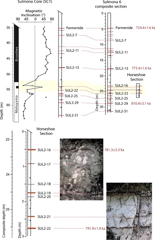
Tephrostratigraphic correlation of the outcropping Sulmona 6 unit with SC1 core (Giaccio et al.2013a), showing the position of the Horseshoe section stratigraphic interval in both successions (yellow area). The lower panel shows a magnification of the stratigraphic log of the Horseshoe section only, with the photographs of the two partially overlapped subsections cropping out at the sampling locality.
The stratigraphic interval investigated in this study crops out about 500 m SE from the SC1 core site (Fig. 1), in a 3-m-thick section that we named the ‘Horseshoe’ section for the discovery of this object at the site. The Horseshoe section consists of whitish faintly laminated to massive, calcareous mud that X-ray diffraction and SEM analyses reveal to be mainly biogenic micrite. This interval also includes seven tephra layers, from SUL2–16 to SUL2–22 (Fig. 2), that can be continuously traced laterally at both outcrop (tens to hundreds metres) and basin (hundreds of metres to kilometres) scales, allowing the unambiguous correlation of the core and the exposed sections. The tephra layers show a homogeneous thickness and tabular-horizontal shape at all of the localities, with a sharp basal contact with the underling calcareous muds. These stratigraphic and lithological features suggest an uniform and very low-energy lacustrine sedimentary environment with no relevant post-depositional disturbances (e.g. erosion, tephra reworking, etc.) and thus a substantial continuity of the sediment accumulation. The section was sampled in its entirety and because the sediment is too friable to be drilled, we collected 46 contiguous hand samples, each spanning 6–16 cm of stratigraphic thickness. The hand samples were oriented in situ using a magnetic compass on a horizontal surface prepared on the top of each block. The tephra layers are only few centimetres thick, and, except for SUL2–19, are too unconsolidated to be sampled. The oriented blocks were then cut in layers of 2 cm thickness, using a band saw, from which we made standard palaeomagnetic cubes of 2 cm on a side. The zero stratigraphic level was placed at the top of the highest sample, which is 53 cm above tephra SUL2–16.
3 METHODS
3.1 Palaeomagnetism and rock magnetism
The palaeomagnetic and rock magnetic properties of at least one sample per layer were measured in the laboratory of the Istituto Nazionale di Geofisica e Vulcanologia. The low-field magnetic susceptibility (k) was measured on an AGICO MFK1-FA kappabridge. The natural remanent magnetization (NRM) was measured using a 2G Enterprises DC SQUIDs superconducting rock magnetometer in a magnetically shielded room. The NRM was stepwise demagnetized by translating the samples through a set of three orthogonal alternating field (AF) coils mounted in-line on the 2G Enterprises system. For AF demagnetization we used 13 steps up to 100 mT. After AF demagnetization of the NRM, an anhysteretic remanent magnetization (ARM) was produced by simultaneous application of an AF peak of 100 mT and a direct current (dc) bias field of 0.05 mT, translating the samples through the AF and dc coil system at a speed of 10 cm s–1. The ARM was then AF demagnetized in 11 steps up to 100 mT. For 36 specimens, distributed throughout the section, we also carried out a stepwise thermal demagnetization, in 10–11 steps up to 450 °C. The analysis of the demagnetization data was carried out by using the DAIE software (Sagnotti 2013). A characteristic remanent magnetization (ChRM) was isolated for all the measured specimens and its direction was computed by principal component analysis (Kirschvink 1980) using at least four consecutive demagnetization steps, and the maximum angular deviation (MAD) was determined for each computed ChRM direction (Table S1).
The relative palaeointensity (RPI) variation of the geomagnetic field in the Horseshoe section was estimated by normalizing the NRM intensity that remained after 20 mT AF, that is after complete removal of the normal overprint, by the ARM intensity measured at the same demagnetization level (NRM20mT/ARM20mT).
In order to identify the main remanence carriers, for selected samples we measured hysteresis properties in cycles up to 1 T, as well as isothermal remanent magnetization (IRM) acquisition curves, followed by backfield remagnetization curves and first order reversal curves (FORC; Roberts et al.2000) to estimate the domain magnetic state, the coercivity distribution and the degree of magnetic interaction of the magnetic minerals population. All of the measurements were carried out by a Princeton Measurement Corporation Micromag 2900. In order to identify the Curie temperatures of the main magnetic minerals and to check the possible occurrence of significant alteration during heating, we also measured the variation of magnetic susceptibility in heating-cooling cycles between room temperature and 700 °C, using a AGICO CS-3 apparatus coupled to a MFK1-FA kappabridge (Hrouda 1994).
3.2 40Ar/39Ar dating of tephra layers
Pristine sanidine crystals from SUL2–15, SUL2–16 and SUL2–22 tephra layers were handpicked under a binocular microscope and then slightly leached for 5 min in a 7 per cent HF acid solution in order to remove groundmass that might be attached to them. In order to obtain robust chronological constraints, a subset of crystals from samples SUL2–15 and SUL2–22, prepared at Gif laboratory, were sent to the Berkeley Geochronology Center (BGC) for separate irradiation and analysis. Several proposed calibrations of the 40Ar/39Ar chronometer are currently in use, which yield ages that vary by ∼2 per cent in the time range of the M-B reversal. Rather than absolute ages, the results presented here are instead concerned with time intervals, which are insensitive to the calibration used. Accordingly, we report ages relative to the ACs age of 1.194 Ma (Nomade et al.2005) and the decay constants of Steiger & Jäger (1977) without necessarily endorsing these values.
3.3 Gif analyses
About 40 crystals from SUL2–15, SUL2–16 and SUL2–22 tephras were loaded in a single hole hosted in an aluminium disc and irradiated for 30 min (IRR50) in the β1 tube of the OSIRIS reactor (CEA Saclay, France). After irradiation, single crystals were individually placed in a stainless steel sample holder and then loaded into a differential vacuum Cleartran® window. Single crystals were fused at about 15 per cent of the full laser power using a 25 W CO2 laser (Synrad®). Ar isotopes were analysed using a VG5400 mass spectrometer equipped with a single ion counter (Balzers® SEV 217 SEN) following procedures outlined in Nomade et al. (2010). Each Ar isotope measurement consists of 20 cycles of peak switching of the argon isotopes. Neutron fluence (J) was monitored by co-irradiation of Alder Creek Sanidine (ACs-2, Nomade et al.2005) placed in the same pit as the sample. J values were determined from analyses of three ACs-2 single grains for each sample.
Procedural blanks were measured every three or four crystals (Table S2). The precision and accuracy of the mass discrimination correction was monitored by daily measurements of air argon at various pressures (see full experimental description in Nomade et al.2010). Nucleogenic production ratios used to correct for reactor produced Ar isotopes from K and Ca are given in Table S2.
3.4 BGC analyses
Samples analysed at the BGC were irradiated for 3 hr in the cadmium-lined CLICIT facility of the TRIGA reactor at Oregon State University. Neutron fluence was monitored by ACs standards in 6 and 4 positions (for SUL2–15 and SUL2–22, respectively) bracketing the samples, and J-values for each position were determined by the weighted mean of five to six analyses each comprising five grains of ACs. J-values for each of the samples was determined by a planar fit to the standard data.
Mass spectrometry used an MAP 215–50 mass spectrometer with a single analogue electron multiplier. Data were acquired in 15 cycles of peak-hopping, and relative isotope abundances were determined by regression to an empirically determined equilibration time. Mass discrimination (1.01176 ± 0.00106 per Dalton) was corrected using the methods of Renne et al. (2009) based on 37 air pipettes interspersed with the samples and standards. Procedural blanks were measured every two to three samples and standards, and their mean and standard deviation were applied for correction. Nucleogenic production ratios used to correct for reactor produced Ar isotopes from K and Ca are given in the Table S3.
4 RESULTS
4.1 Palaeomagnetism
The results indicate that both AF and thermal demagnetization treatments provide consistent results and allow the identification of a well-defined ChRM (MAD values <5 °) for most of the specimens, and straightforward demagnetization plots for all the samples collected from the upper 250 cm of the Horseshoe section (Fig. 3). The reconstructed ChRM declination, inclination and MAD stratigraphic trends are shown in Fig. 4 and listed in Table S1. In the upper part of the section (from 0 to 152 cm), all of the samples record normal polarity, with data aligned towards the origin of vector demagnetization diagrams after the removal of a magnetic overprint in AF < 20 mT (Fig. 3a). Following removal of a normal overprint in AF < 20 mT, samples below 152 cm mostly record a clearly defined reverse ChRM (Figs 3b and 4). A few samples from thin layers immediately above tephras SUL2–19 and SUL2–20 show a normal polarity ChRM, with demagnetization diagrams analogous to those measured for samples above 152 cm (Figs 3c and 4). Interestingly, the sample collected from tephra SUL2–19 records reverse polarity (Fig. 3d). Below 250 cm, palaeomagnetic data are of difficult interpretation. For these samples a very weak signal remains after removal of the normal overprint at AF steps < 20 mT. In some specimens, it seems that the NRM left after AF 20 mT is of normal polarity (Fig. 3e). In other samples, a reverse component can be recognized at higher AF steps (Fig. 3f). In all cases, the ChRM for samples below 250 cm is poorly defined and characterized by high MAD values (Fig. 4).
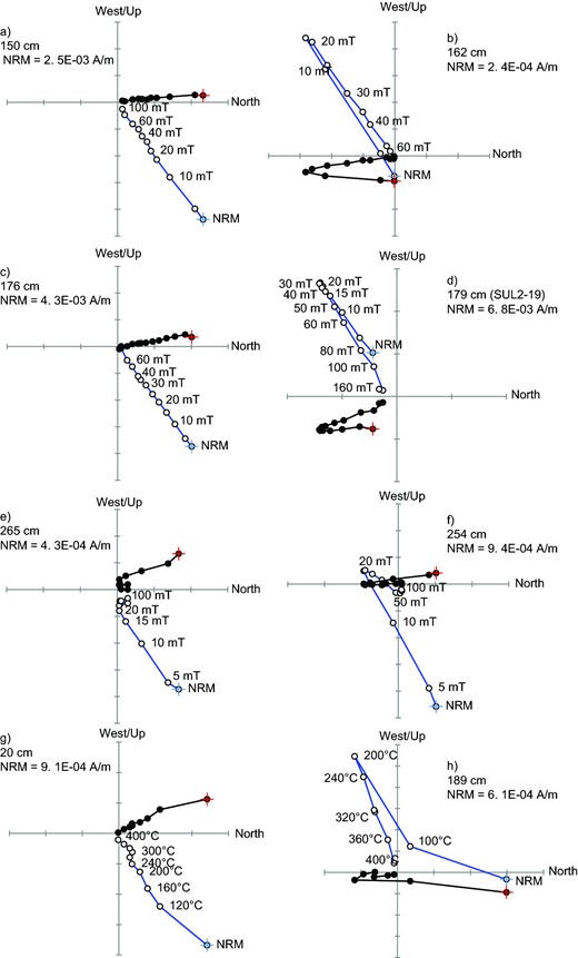
Representative orthogonal demagnetization vector diagrams for selected specimens of the Horseshoe section. Black (white) circles indicate projection on the horizontal (vertical) plane. The natural remanent magnetization (NRM) projections are marked by a cross superimposed on the circles. The numbers close to the symbols for the vertical planes projections indicate the level of stepwise demagnetization. Plots a–f refer to samples subjected to AF demagnetization, plots g-h refer to samples subjected to thermal demagnetization.
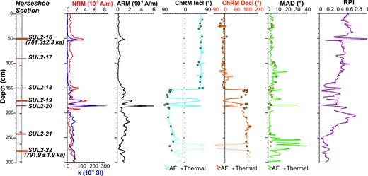
Stratigraphic variation of the rock magnetic and palaeomagnetic parameters measured in the Horseshoe section. Samples below 250 cm are characterized by poorly defined ChRM directions.
Thermal demagnetization data are consistent with those obtained by the AF treatment; the normal magnetic overprint is removed at 200 °C, and a ChRM can be determined between 200 and 450 °C, which is the temperature at which all the samples are almost completely demagnetized (Figs 3g and h).
The palaeomagnetic data from the normal polarity samples above 152 cm are tightly grouped around a mean ChRM direction of Decl = 354.9 °, Incl = 65.1 °, with statistical dispersion parameters of k = 51.2 and α95 = 2.1 °. Below 152 cm, the samples are mostly of reverse polarity, indicating that the sequence was deposited during the latest Matuyama Chron. The Fisherian statistics for the clearly reverse ChRM directions measured below 152 cm indicate a mean ChRM of Decl = 168.9 °, Incl = –58.9 °, with k = 30.3 and α95 = 3.8 °.
The RPI record shows the presence of two intervals of RPI low, at 140–185 cm and from 245 cm to the base the section (Fig. 4).
4.2 Rock magnetism and identification of the magnetic carriers
The rock magnetic parameters dependent on the concentration of magnetic minerals indicate a fairly uniform distribution in the lacustrine sediments, with sharp positive peaks limited to samples collected on top of tephra layers SUL2–16, SUL2–18, SUL2–19 and SUL2–20 (Fig. 4). The typical lacustrine samples are characterized by low coercivity minerals, with steep IRM acquisition curves at pulse fields <0.1 T and a saturation IRM (SIRM) value reached in fields of about 0.2 T (Figs 5a–c). The FORC diagrams show a coercivity distribution typical of stable single domain (SD) grains, with closed contours and a peak around Hc values of about 20 mT (Figs 6a–c). Conversely, the samples collected on top of tephra layers SUL2–19 and SUL2–20 are characterized by a higher coercivity, with IRM values far from saturation at 0.2T (with IRM approaching saturation at 0.6–0.8 T, Fig. 5d) and their FORC diagram shows a coercivity distribution with a peak close to the origin and a long tail extending beyond 100 mT along the Hc axis (Fig. 6d). Thermomagnetic curves obtained on critical samples are shown in Fig. 7. Even if the magnetic susceptibility values are low and the thermomagnetic curves are noisy, a major drop in the heating curves can be clearly recognized, indicating the Curie temperature of the main magnetic minerals. This drop occurs sharply between 520 and 580 °C in specimens HS31_3 and HS32_1 (Figs 7b and d), collected just above and below the M-B polarity flip, and indicates that magnetite is the main magnetic phase in these specimens. Moreover, for these specimens the cooling curves are well above the heating curves (Figs 7a and c), suggesting a significant alteration during heating with production of new magnetite particles from the non-magnetic matrix. The susceptibility drop in the heating curve of specimen HS35B_1 develops smoothly between 380 and 550 °C (Fig. 7f). Moreover, the heating and cooling curves for this specimen are nearly reversible (Fig. 7e), suggesting that very limited alteration occurred during the thermomagnetic cycle.
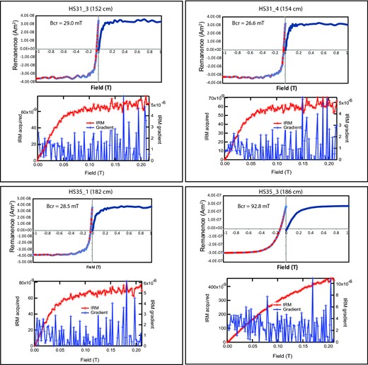
Isothermal remanence (IRM) acquisition curves and back field remagnetization curves for four representative specimens. Samples HS31_3 and HS31_4, collected at 152 and 154 cm of stratigraphic depth are just above and below the 180 ° directional switch of the B-M reversal. Typical lacustrine sediments (HS31_3, HS31_4 and HS35_1) are characterized by properties indicative of low-coercivity ferrimagnetic minerals, such as magnetite, with steep IRM acquisition curves in fields <0.1 T and saturation of IRM reached in fields of about 0.2 T. For these sediments, the coercivity of remanence (Bcr) ranges between 25 and 30 mT. Conversely, sample HS35_3, which was collected just on top of tephra SUL2–20 shows a distinctly higher coercivity, with a Bcr of about 93 mT and saturation of the IRM reached in fields >0.5 T.
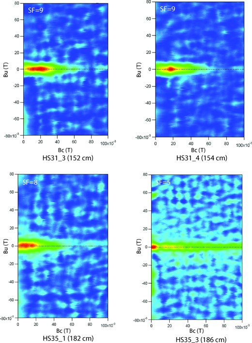
First order reversal curve (FORC) diagrams for the same representative specimens discussed in Fig. 5. The FORC data have been processed using the FORCinel software (Harrison & Feinberg 2008). SF, smoothing factor. Lacustrine sediments samples are characterized by a coercivity distribution with almost closed contours peaked at coercivity Bc of about 15–25 mT. The FORC diagram for the sample HS35_3, just on top of tephra SUL2–20, shows a restricted peak close to the origin and a long tail along the Bc axis, extending beyond 100 mT.
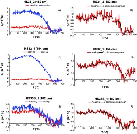
Variation of total susceptibility kT (sensu Hrouda 1994) during a heating-cooling cycle between room temperature and 700 °C for two specimens immediately above (a: specimen HS31_3, collected at 152 cm stratigraphic depth) and below (c: specimen HS32_1, collected at 154 cm stratigraphic depth) the M-B transition and for a specimen collected immediately above tephra SUL2–19 (e: specimen HS35B_1, collected at 182 cm stratigraphic depth). Measurements were carried out in air and both heating and cooling curves are corrected for the empty furnace. Diagrams on the right-hand side (b, d, f) show a magnification of the heating curves only.
Overall, the rock magnetic data demonstrate that specimens collected just above and below the M-B polarity flip are remarkably homogeneous and indicate that the magnetic carrier consists of nearly stoichiometric magnetite, whereas specimens collected immediately above tephras SUL2–19 and SUL2–20 have a slightly different composition with regards to both the magnetic and the non-magnetic fractions.
4.3 40Ar/39Ar dating
Age-probability density spectra for tephras SUL2–15, SUL2–16 and SUL2–22 are presented in Fig. 8. Weighted mean ages and corresponding uncertainties are calculated using IsoPlot 3.0 (Ludwig 2003) and are given at the 2σ level. Full analytical details for individual crystals are given in Tables S2 and S3.
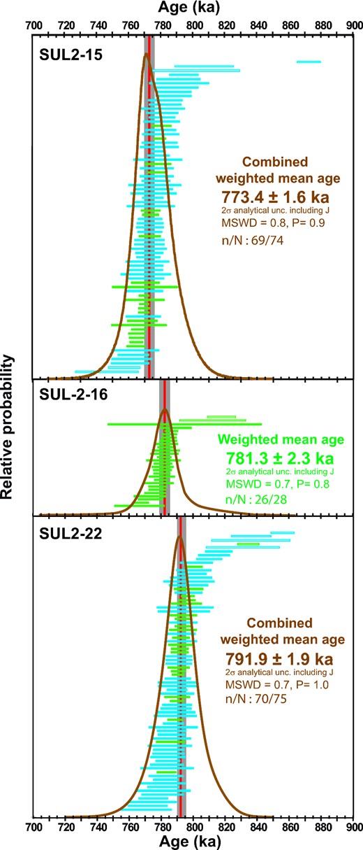
Age-probability density spectra and individual crystal age for SUL2–15, SUL2–16 and SUL2–22 tephra layers. Blue and green boxes (1σ) are crystals analysed at the Berkeley Geochronology Center and Gif Sur Yvette, respectively.
At Gif, a total of 21, 28 and 22 crystals were dated for SUL2–15, SUL2–16 and SUL2–22, respectively. These three tephra layers are dominated by juvenile crystals and only a few xenocrysts were found in SUL 2–16 and SUL 2–22. The crystals belonging to the most probable mode of each tephra yielded eruption ages (weighted mean of the all the juvenile crystals) of 771.3 ± 2.0, 781.3 ± 2.3 and 792.6 ± 2.4 ka for SUL2–15, SUL2–16 and SUL2–22, respectively. Corresponding inverse isochron ages are identical within uncertainty and display atmospheric 40Ar/36Ar initial intercepts.
At BGC, a total of 53 crystals were dated and yielded weighted mean ages of 776.8 ± 2.7 and 790.9 ± 2.8 ka for SUL2–15 and SUL2–22, respectively, excluding obvious xenocrysts from each population. For both SUL2–15 and SUL2–22, the results from the two labs are indistinguishable at 95 per cent confidence and we combine both data sets to obtain weighted mean ages of 773.4 ± 1.6 and 791.9 ± 1.9 ka, respectively.
Interpolation of our age versus stratigraphic height data for samples SUL2–16 and SUL2–22 yields an age of 786.1 ± 1.5 ka (2σ, analytical uncertainty) for the M-B boundary according to the nominal calibration we used and assuming constant sedimentation rates (max. and min.) allowed by the age uncertainties of the two tephra layers. Other currently used calibrations applied to our data yield ages ranging from ∼781 ka (Rivera et al.2013) to ∼794 ka (Renne et al.2011), all significantly older than the age of 773.1 ± 0.8 ka estimated by Channell et al. (2010).
5 DISCUSSION
The lacustrine sediments of the SUL6 unit are characterized by excellent palaeomagnetic properties, allowing the reconstruction of the M-B polarity transition in very fine detail. The strong correlation and consistency between the rock magnetic and palaeomagnetic stratigraphic trends between the Horseshoe section and SC1 core demonstrate the lateral continuity of the experimental results, and point out the reliability of the palaeomagnetic signal for high-resolution geomagnetic reconstructions.
In the Horseshoe section, the rock magnetic and palaeomagnetic data are consistent with magnetite being the main carrier of the remanence and indicate that the concentration of magnetic minerals is generally uniform throughout the sequence. Sharp and high peaks of concentration-dependent rock magnetic parameters are only measured in thin (2–6 cm thick) layers deposited on top of tephras SUL2–19 and SUL2–20 (Fig. 4).
The 180 ° polarity flip associated to the M-B polarity transition occurs sharply between two adjoining levels (at 152 and 154 cm of stratigraphic depth, respectively) cut from the same hand block, and it is recorded consistently between seven independent samples (four from the 152 cm level and three from the 154 cm level) and with both AF and thermal demagnetization treatments (Fig. 9). The M-B magnetic reversal is recorded a few cm below tephra SUL2–18 (Fig. 9). SUL2–18 is a very thin tephra (ca. 2 mm thick) made of fine ash mostly composed by glass shards. Due to its petrographic character and stratigraphic position, we consider highly unlikely that the SUL2–18 tephra may have caused any disturbance of the M-B reversal recording. The 180 ° polarity flip occurs during the uppermost part of the younger RPI minimum, with a distinct RPI recovery following the directional reversal. Below 154 cm, two other sharp transitions to normal ChRM directions are recorded for the samples collected immediately above tephra layers SUL2–19 and SUL2–20 (Fig. 4). These transitions are limited to the thin stratigraphic intervals just on top of tephra layers SUL2–19 and SUL2–20 (namely, at 172–176 cm on top of SUL2–19 and at 184–186 cm on top of SUL2–20; Fig. 9). They correspond to intervals of increased concentration of magnetic minerals and different magnetic mineralogy (Figs 4–7). We thus conclude that these intervals were remagnetized after the M-B reversal. Another interval of possible normal polarity is recorded by the poorly defined ChRM directions between about 260 and 275 cm (Fig. 4), where a very weak palaeomagnetic signal left after removal of the normal overprint. This interval corresponds to the older identified RPI minimum. This RPI minimum is interpreted as a characteristic feature of the geomagnetic reversal process (sensu Valet et al.2012) and could correspond to the previously documented geomagnetic precursor of the M-B reversal (e.g. Hartl & Tauxe 1996; Dinarés-Turell et al.2002; Jin et al.2012).
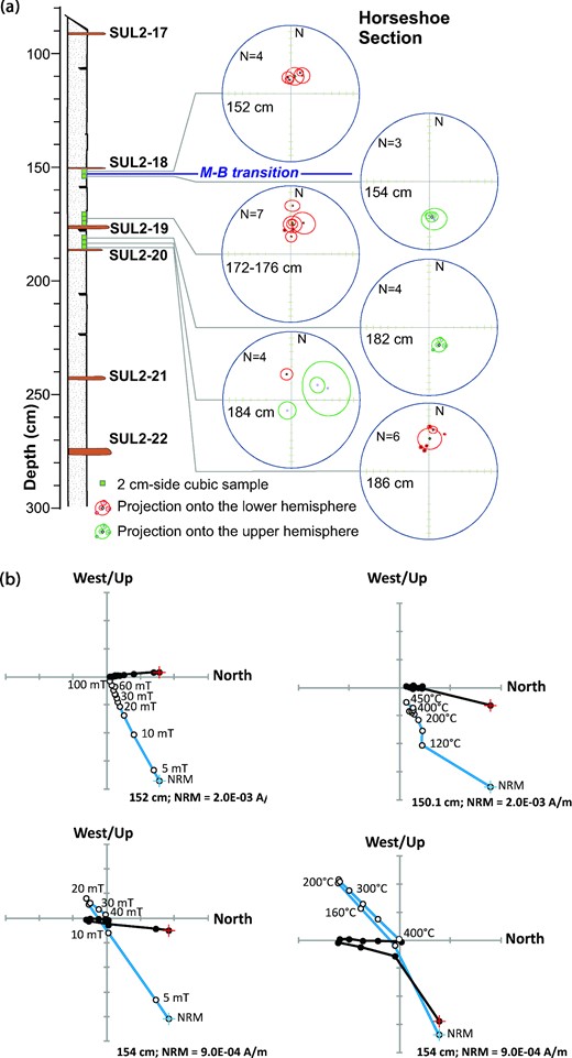
(a) Equal-area projections of the ChRM directions, and related α95 confidence cones, for selected samples from critical stratigraphic intervals of the Horseshoe section. (b) Representative orthogonal demagnetization vector diagrams for samples collected across the M-B transition. Black (white) circles indicate projection on the horizontal (vertical) plane. The natural remanent magnetization (NRM) projections are marked by a cross-superimposed on the circles. The numbers close to the symbols for the vertical plane projections indicate the level of stepwise demagnetization. Diagrams refer both to AF (left-hand panel) and thermal (right-hand panel) stepwise demagnetization treatments.
New high precision 40Ar/39Ar dates obtained on three tephra layers (SUL2–15, SUL2–16 and SUL2–22), along with those already published (Giaccio et al.2013a), provide tight chronological constraints for the Sulmona succession and indicate average sedimentation rates in the range of 20–25 cm ka−1 during the 720–810 ka interval (Fig. 10). The 40Ar/39Ar ages for the SUL2–16 (781.3 ± 2.3 ka, 2σ analytical uncertainty) and SUL2–22 (791.9 ± 1.9 ka, 2σ analytical uncertainty) tephras, indicate that the stratigraphic interval bracketing the M-B transition deposited in ca. 10.6 ± 2.98 ka, with a mean sedimentation rate of about 21 cm ka–1 (Fig. 9). This implies a centennial temporal resolution for the Horseshoe palaeomagnetic record (2 cm = ca. 100 a).
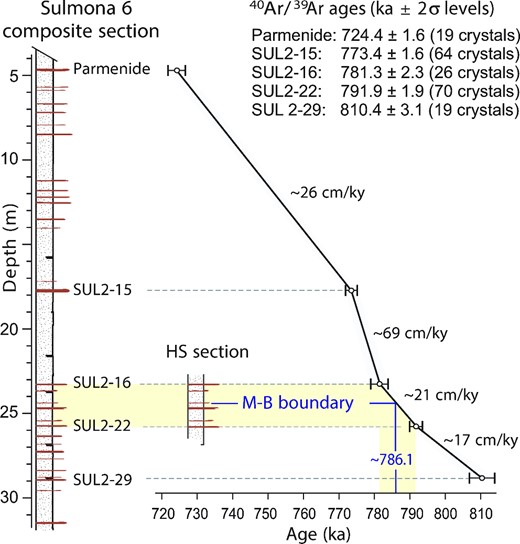
Age versus depth for the Sulmona 6 unit and estimated sedimentation rates, computed by linear interpolation between two consecutive dated tephra layers. The yellow area indicates the depth and age intervals spanned by the uppermost and the lowermost dated tephras (SUL2–16 and SUL2–22) in Horseshoe section. The stratigraphic position and the extrapolated age (±2σ level) of the M-B geomagnetic field reversal are also shown.
Taking into account that: (1) we have no sampling gap around the M-B polarity transition, (2) all the measured samples at 152 cm and above show a normal polarity ChRM, (3) all the measured samples at 154 cm and below show a reverse polarity ChRM, (4) we do not observe any sample with intermediate ChRM directions and (5) there is no evidence of a stratigraphic gap in this interval and the magnetic mineralogy is constant through the reversal record, we conclude that the directional 180 ° flip must have occurred within the thin (<2 cm) interval centred on 153 cm and therefore lasted much less than a century. Even if age and duration of the magnetic reversal may vary significantly between different sites on the globe, the transition duration we retrieved is one order of magnitude shorter than what it is predicted by previous reconstructions of the M-B transitional field (Leonhardt & Fabian 2007). This difference can be explained by a chronologic bias in the input data set used in modelling, which strongly relies on marine cores with an order of magnitude resolution lower than our record and on u-channel measurements that may drastically smooth an originally sharp geomagnetic signal (Roberts 2006).
In the Horseshoe section, the duration of the younger RPI minimum, spanning about 45 cm and including the M-B polarity transition, can be estimated at about 2.4 ka. The older RPI minimum is recorded at depths >245 cm, and from correlation to the data collected on the SC1 core we estimate that its overall stratigraphic thickness spans about 50 cm. We estimate that this first RPI minimum also lasted about 2.5 ka and ended 3.2 ka before the start of the younger RPI minimum (Fig. 11). According to our age model, the age of this RPI minimum is centred around 793 ka, in general agreement with former age estimates of the M-B precursor from lavas in Tahiti, Chile and La Palma (Singer 2014), as well as from marine sediments (Kent & Schneider 1995; Yamazaki & Oda 2001), the Chinese loess (Jin et al.2012) and the Dome C ice core (Dreyfus et al.2008). Our results differ from those of Channell et al. (2010) and Singer (2014) regarding the age of the directional polarity flip itself, which they inferred to occur at 773.1 ± 0.8 and 776 ± 2 ka, respectively. The most conservative implication of our data is that this flip occurred prior to the eruption and deposition of tephra layer SUL2–16 at 781.3 ± 2.3 ka. As discussed previously, the interpolated age based on our nominal calibration (786.1 ± 1.5 ka) for the M-B reversal is greater than ∼781 ka, for any credible calibration of the 40Ar/39Ar geochronometer, and is thus distinctly older than the estimates of either Channell et al. (2010) or Singer (2014). Our Sulmona-based age estimate for the M-B reversal is in fact less model dependent than those based on astronomically tuned marine ice volume models (e.g. Channell et al.2010), and provides higher precision than is normally attainable by 40Ar/39Ar dating of whole-rock samples of lavas that sample the geomagnetic field only episodically (e.g. Singer 2014). For these reasons we suggest that the Sulmona record offers the currently most reliable age for the M-B reversal, although the age is subject to resolution of 40Ar/39Ar calibration issues.
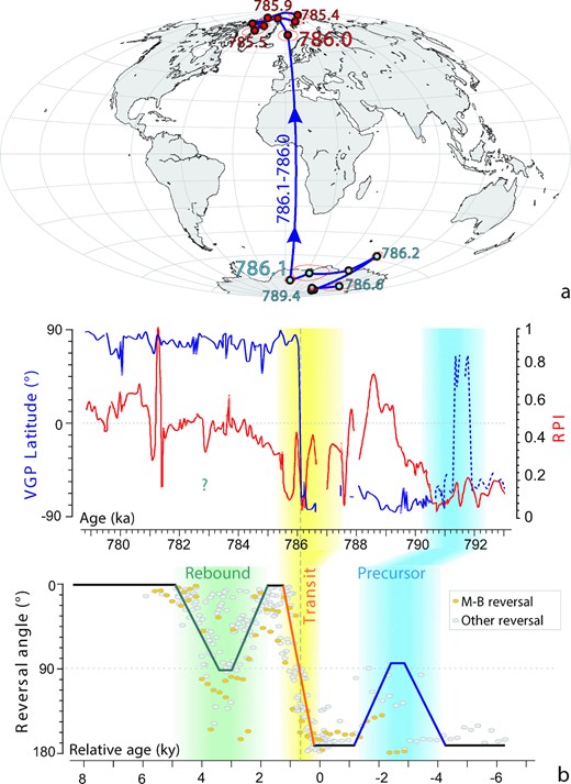
(a) Virtual geomagnetic pole (VGP) path reconstructed for the palaeomagnetic data from the discrete specimens around the M-B transition in the Horseshoe section. (b) Stratigraphic trends for the VGP latitude (blue curve) and RPI scaled to unit maximum (red curve) for the Horseshoe section compared with the schematic reversal path of Valet et al. (2012), from compilation of reversal records in data flows, illustrating the succession of the reversal precursor, polarity switch and rebound. Coloured area in the Horseshoe plot indicates the stratigraphic intervals of minimum RPI that have been correlated with the precursor and the transit phases of the Valet et al. (2012) scheme.
6 CONCLUSIONS
The Sulmona lacustrine sequence preserves a high-resolution record of the M-B geomagnetic field reversal. The retrieval of continuous reliable palaeomagnetic properties from discrete samples and of high precision 40Ar/39Ar dates from several distributed tephra layers provides an unprecedented opportunity to estimate the tempo, rate and dynamics of the reversal process. In particular, the centennial-scale M-B record from the Sulmona lacustrine sequence supports early claims for the occurrence of extremely fast magnetic directional change during geomagnetic field reversals (i.e. the RTFC hypothesis), whose experimental evidence was hitherto limited to Miocene lava flows from the United States. This study reports the first sedimentary record providing compelling evidence for a very high rate (>2 °/a) of the directional change during the M-B polarity reversal.
The lack of intermediate directions recorded during the M-B transition indicates that even with continuous palaeomagnetic sampling, it will not be possible to retrieve the details of the transition in sequences with a sedimentation rate lower than 20 cm ka−1.
The reconstruction of the overall M-B transitional period, with a reversal precursor and a main transition phase with a 180 ° polarity switch, is consistent with the reconstruction of the dynamics of geomagnetic field reversals provided by Valet et al. (2012). According to this study, the estimated duration of the instability associated with the reversal precursor is about 2.5 ka, with a time lag of about 3 ka between the precursor and the directional transit phase (Fig. 11). Both estimates are consistent with the results we obtained from the Sulmona lacustrine sequence. Valet et al. (2012) also estimated that the actual directional transit between the two opposite polarities lasted less than 1 ka (Fig. 11). The data from the Sulmona basin allow us now to substantially refine this assessment, indicating that the 180 ° polarity switch actually was very rapid. Specifically, the lack of intermediate directions recorded during the M-B transit indicates that even our continuous and centennial-scale palaeomagnetic record was not able to retrieve the details of the transition. Therefore, the polarity reversal occurred in a time considerably shorter than the temporal resolution of the Sulmona record, which is in a fraction of a century.
We are very grateful to Angelo Alfredo Scipione and Arnaldo Scipione for their valuable help during preparation of the samples and for the use of their carpentry shop in Sulmona for cutting hand samples into precise palaeomagnetic cubes. The manuscript was improved by the constructive reviews by Rob Coe and Darren Mark. The geochronological part of this work was supported by the INSU-SYSTER action (2013) and by the Ann and Gordon Getty Foundation (BGC).
REFERENCES
SUPPORTING INFORMATION
Additional Supporting Information may be found in the online version of this article:
Table S1. Rock magnetic and palaeomagnetic properties of samples from the Horseshoe section.
Table S2. Full 40Ar/39Ar data set for individual crystals measured at the Gif SurYvette facility (France).
Table S3. Full 40Ar/39Ar data set for individual crystals measured at the Berkeley Geochronology Center (USA) (Supplementary Data).
Please note: Oxford University Press is not responsible for the content or functionality of any supporting materials supplied by the authors. Any queries (other than missing material) should be directed to the corresponding author for the article.
